Casimir piston for massless scalar fields
in three dimensions

We study the Casimir piston for massless scalar fields obeying Dirichlet boundary conditions in a three dimensional cavity with sides of arbitrary lengths $a,b$ and $c$ where $a$ is the plate separation. We obtain an exact expression for the Casimir force on the piston valid for any values of the three lengths. As in the electromagnetic case with perfect conductor conditions, we find that the Casimir force is negative (attractive) regardless of the values of $a$, $b$ and $c$. Though cases exist where the interior contributes a positive (repulsive) Casimir force, the total Casimir force on the piston is negative when the exterior contribution is included. We also obtain an alternative expression for the Casimir force that is useful computationally when the plate separation $a$ is large.

1 Introduction

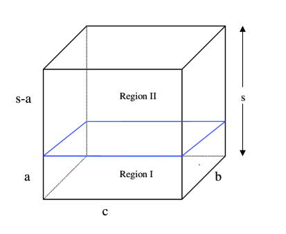
Figure 1: Casimir piston in three dimensions.

Two years ago, in an interesting paper [1], the Casimir piston was studied for a two-dimensional scalar field obeying Dirichlet boundary conditions on a rectangular region. Among other things, it was shown that the Casimir force on the piston is always attractive (negative) regardless of the ratio of the two sides. In this paper, we study the three-dimensional Casimir piston for massless scalar fields. A Casimir piston in three dimensions is depicted in Fig. 1. We choose the base to be a $b\times c$ rectangular region and $a$ to be the plate separation (the distance from the base to the piston). The piston divides the volume into two regions. We refer to region I as the interior and region II as the exterior. Both regions contribute to the Casimir force on the piston. The Casimir piston therefore modifies some previous standard Casimir results [2] where the effects of the exterior region are not included.

The Casimir piston for the electromagnetic field with perfect-conductor conditions in a three-dimensional rectangular cavity (box) was studied recently [3] and it was shown that the Casimir force on the piston is again attractive (in contrast to results without exterior region where the force could be positive). The piston for perfect-conductor conditions including the effects of temperature was studied further in [4, 5, 6] where among other things, the long and short distance behavior of the free energy was investigated. A theorem was obtained in [7], where it was shown that the Casimir force between two bodies related by reflection is always attractive, independent of the exact form of the bodies or dielectric properties. This theorem was then generalized further in [8] where it was shown that reflection positivity implies that the force between any mirror pair of charge-conjugate probes of the quantum vacuum is attractive. Attraction does not occur in all Casimir piston scenarios. In a recent paper [9], the Casimir piston for a weakly reflecting dielectric was considered and it was shown that though attraction occurred for small plate separation, this could switch to repulsion for sufficiently large separation. Moreover, for thick enough material, the force remained attractive for all plate separations in agreement with the results in [3]. Two recent preprints [10, 11] also discuss scenarios where repulsive Casimir forces in pistons can be achieved.

For the case of a massless scalar field in a three-dimensional cavity, approximate expressions for the Casimir force were obtained valid for small plate separation [3]. In this paper, we consider the general case of arbitrary lengths. We present exact expressions for the Casimir force on a piston due to a massless scalar field obeying Dirichlet boundary conditions in a three-dimensional box with sides of arbitrary lengths $a,b$ and $c$. We find that the Casimir force on the piston is negative and runs from $-\infty$ (in the limit $a\!\to\!0$) to $0$ (in the limit $a\!\to\!\infty$). For small plate separation $a$, we recover the results found in [3]. We also obtain an exact alternative expression for the Casimir force that is useful computationally when the plate separation is large. We focus our attention on Dirichlet instead of Neumann boundary conditions because it is the more interesting case of the two. It is clear that Neumann boundary conditions will yield a negative Casimir force since the contribution from both the interior and exterior are negative. It is not a priori obvious that in the Dirichlet case the Casimir force will be negative because there exists values of the ratios $a/c$ and $b/c$ where the interior contributes a positive (repulsive) Casimir force. It is therefore interesting to see that in such cases the exterior contributes a negative force of larger magnitude with the important consequence that the total Casimir force is negative. It is worth mentioning that the study of massless scalar fields is not only of theoretical interest but has direct relevance to physical systems such as Bose-Einstein condensates [12, 13, 14].

The Casimir energy can be viewed as the energy with boundary conditions (a sum over discrete modes) minus the energy without boundary conditions (a volume integral over continuous modes). The sum over the discrete modes can typically be decomposed into a volume divergent term (the continuum part that can be subtracted), a surface divergent term and a finite part. In previous set-ups without region II, finite results were obtained by throwing out the surface divergent term. Though the finite results agreed with the zeta function regularization technique, there is nothing that can physically justify throwing out the surface term. It yields a cut-off dependent Casimir force that cannot be removed via a renormalization of the physical parameters of the theory [15, 16, 17]. The agreement between zeta function regularization and cut-off technique (with surface term thrown out) occurs because the zeta function technique in effect renormalizes the surface term to zero. The Casimir piston resolves this issue satisfactorily by having the exterior and interior contributions to the surface divergence cancel. This has been demonstrated in Refs.[1, 3] and we assume this cancellation to hold here. One can simply calculate the Casimir force $F_{1}$ and $F_{2}$ on the piston due to region I and II respectively without including the cut-off dependent terms. The total Casimir force on the piston can then be obtained by adding $F_{1}$ and $F_{2}$. One must just keep in mind that $F_{1}$ and $F_{2}$ actually have cut-off dependent terms but that they cancel when the two are added.

There are two positive aspects to the Casimir piston: the exterior is now included in the calculation of the Casimir force (we add $F_{2}$ to $F_{1}$) and the surface divergence is handled via a cancellation procedure instead of simply throwing it out.

We work in units where $\hbar=c=1$ ($c$ is the speed of light). Note that from now on, when the variable $c$ appears in the text, it always refers to one of the lengths of the base (see Fig. 1).

2 Casimir piston in three dimensions: exact results

The Casimir energy $E_{D}$ for massless scalar fields in a $d$-dimensional box of arbitrary lengths $L_{1},...,L_{d}$ obeying Dirichlet boundary conditions can be conveniently expressed as an analytical part – composed of Riemann zeta and gamma functions – plus a sum of over Bessel functions (eq. (A.12) ; see appendix A and Refs.[18, 23]):

$$E_{D}=\dfrac{\pi}{2^{d+1}}\sum_{j=0}^{d-1}(-1)^{d+j}\,\,\xi^{\,d-1}_{\,k_{1},..,k_{j}}\,\Big{\{}\dfrac{L_{k_{1}}\ldots L_{k_{j}}}{(L_{d})^{j+1}}\Big{(}\Gamma(\tfrac{j+2}{2})\,\pi^{\frac{-j-4}{2}}\,\zeta(j+2)+R_{j}\Big{)}\,\Big{\}}$$ (2.1)

where $R_{j}$ represents the sum over modified Bessel functions $K_{\nu}$:

$$R_{j}=\sum_{n=1}^{\infty}\,\sideset{}{{}^{\prime}}{\sum}_{\begin{subarray}{c}l_{i}=-\infty\\ i=1,\ldots,j\end{subarray}}^{\infty}\dfrac{2\,\,n^{\frac{j+1}{2}}}{\pi}\,\dfrac{\,K_{\frac{j+1}{2}}\big{(}\,2\pi\,n\,\sqrt{(\ell_{1}\frac{L_{k_{1}}}{L_{d}})^{2}+\cdots+(\ell_{j}\,\frac{L_{k_{j}}}{L_{d}})^{2}}\,\,\,\big{)}}{\left[(\ell_{1}\frac{L_{k_{1}}}{L_{d}})^{2}+\cdots+(\ell_{j}\frac{L_{k_{j}}}{L_{d}})^{2}\right]^{\tfrac{j+1}{4}}}\,\,.$$ (2.2)

The prime in the sum for $R_{j}$ means that the case where all $\ell$’s are simultaneously zero is excluded. Note that $R_{j}$ is a function of the ratios of the lengths. In (2.1), there is an implicit summation over the integers $k_{i}$. The symbol $\xi^{\,d-1}_{\,k_{1},..,k_{j}}$ is defined as

$$\xi^{\,d-1}_{\,k_{1},..,k_{j}}=\begin{cases}1&\,\,\mbox{if}\,\,k_{1}\!<\!k_{2}\!<\!\ldots\!<k_{j}\,;\,1\leq k_{j}\leq d-1\\ 0&\,\,\mbox{otherwise}\,\,.\end{cases}$$ (2.3)

The above symbol apparently does not have a name and we refer to it as the $ordered$ symbol in Appendix A. The ordered symbol ensures that the implicit sum over the $k_{i}$ in (2.1) is over all distinct sets $\{k_{1},\ldots,k_{j}\}$, where the $k_{i}$ are integers that can run from $1$ to $d-1$ inclusively under the constraint that $k_{1}\!<\!k_{2}\!<\!\cdots\!<k_{j}$. The superscript $d\!-\!1$ specifies the maximum value of $k_{j}$. For example, if $j=2$ and $d=4$ then $\xi^{\,d-1}_{\,k_{1},..,k_{j}}=\xi^{\,3}_{\,k_{1},k_{2}}$ and the non-zero terms are $\xi_{\,1,2}$ , $\xi_{\,1,3}$ and $\xi_{\,2,3}$. This means the summation is over $\{k_{1},k_{2}\}=(1,2),(1,3)$ and $(2,3)$. Note that the implicit summation over $k_{i}$ is also performed in $R_{j}$ since $R_{j}=R_{j}(L_{k_{1}}/L_{d},..,L_{k_{j}}/L_{d})$. For the special case of $j=0$, $R_{j}$ is defined to be zero and $\xi^{\,d-1}_{\,k_{1},..,k_{j}}$ and $L_{k_{j}}$ are defined to be identically one so that $\xi^{\,d-1}_{\,k_{1},..,k_{j}}\,\frac{L_{k_{1}}\ldots L_{k_{j}}}{(L_{d})^{j+1}}$ = $1/L_{d}$ for $j=0$.

From (2.1) we can readily obtain the Dirichlet Casimir energy in three dimensions ($d=3$):

$$E_{D}=-\dfrac{\pi^{2}}{1440}\,\dfrac{L_{1}\,L_{2}}{L_{3}^{3}}+\dfrac{\zeta(3)}{32\,\pi\,L_{3}^{2}}\big{(}L_{1}+L_{2}\big{)}-\dfrac{\pi}{96\,L_{3}}+R(L_{1},L_{2},L_{3})$$ (2.4)

where $R$ is a function of $L_{1},L_{2}$ and $L_{3}$ and represents the sums over $R_{j}$’s i.e.

$$R(L_{1},L_{2},L_{3})=\dfrac{\pi}{16\,L_{3}^{2}}\Big{[}L_{1}\,R_{1}(L_{1}/L_{3})+L_{2}\,R_{1}(L_{2}/L_{3})\,\Big{]}-\dfrac{\pi\,L_{1}\,L_{2}}{16\,L_{3}^{3}}\,R_{2}(L_{1}/L_{3},L_{2}/L_{3})$$ (2.5)

where $R_{1}(L_{1}/L_{3})$ means that $R_{1}$ is a function of $L_{1}/L_{3}$. The functions $R_{1}$ and $R_{2}$ are sums over modified Bessel functions given by (2.2) i.e.

$$\begin{split}&R_{1}(L_{1}/L_{3})=\sum_{n=1}^{\infty}\sum_{\ell=1}^{\infty}\,\dfrac{4\,n}{\pi\,\ell}\,\frac{L_{3}}{L_{1}}\,K_{1}\Big{(}2\,\pi\,n\,\ell\,\frac{L_{1}}{L_{3}}\Big{)}\\ &R_{2}(L_{1}/L_{3},L_{2}/L_{3})=\sum_{n=1}^{\infty}\,\sideset{}{{}^{\prime}}{\sum}_{\ell_{1},\ell_{2}=-\infty}^{\infty}\!\!\dfrac{2\,n^{3/2}\,K_{3/2}\Big{(}2\,\pi\,n\,\sqrt{\Big{(}\ell_{1}\dfrac{L_{1}}{L_{3}}\Big{)}^{2}+\Big{(}\ell_{2}\dfrac{L_{2}}{L_{3}}\Big{)}^{2}}\,\,\Big{)}}{\pi\left[\Big{(}\ell_{1}\dfrac{L_{1}}{L_{3}}\Big{)}^{2}+\Big{(}\ell_{2}\dfrac{L_{2}}{L_{3}}\Big{)}^{2}\right]^{3/4}}\,.\end{split}$$ (2.6)

The Casimir energy does not depend on which sides are labeled $L_{1}$, $L_{2}$ and $L_{3}$. Expression (2.4) for the Casimir energy is therefore invariant under permutations of the labels $L_{1}$, $L_{2}$ and $L_{3}$ and we are free to label the three sides as we wish. For the Casimir piston depicted in Fig. 1, there are two regions to consider. In region I, the three sides are $a$, $b$ and $c$ and we label them $L_{1}=c$, $L_{2}=b$ and $L_{3}=a$. In region II, the three sides are $s-a$, $c$ and $b$ and we label them $L_{1}=s-a$, $L_{2}=c$ and $L_{3}=b$. The Dirichlet Casimir energy in region I and II is obtained by substituting the corresponding lengths in (2.4):

$$\begin{split}E_{D1}&=-\dfrac{\pi^{2}}{1440}\,\dfrac{b\,c}{a^{3}}+\dfrac{\zeta(3)}{32\,\pi\,a^{2}}(b+c)-\dfrac{\pi}{96\,a}+R(c,b,a)\\ E_{D2}&=-\dfrac{\pi^{2}}{1440}\,\dfrac{(s-a)\,c}{b^{3}}+\dfrac{\zeta(3)}{32\,\pi\,b^{2}}(s-a+c)-\dfrac{\pi}{96\,b}+R(s-a,c,b)\,.\end{split}$$ (2.7)

The function $R(c,b,a)$ is obtained from (2.5) and (2.6):

$$\begin{split}R(c,b,a)&=\dfrac{\pi}{16\,a^{2}}\big{[}c\,R_{1}(c/a)+b\,R_{1}(b/a)\,\big{]}-\dfrac{\pi\,c\,b}{16\,a^{3}}\,R_{2}(c/a,b/a)\\ &\quad=\dfrac{1}{4\,a}\sum_{n=1}^{\infty}\sum_{\ell=1}^{\infty}\,\dfrac{n}{\ell}\,\Big{[}K_{1}\big{(}2\,\pi\,n\,\ell\,c/a\big{)}+K_{1}\big{(}2\,\pi\,n\,\ell\,b/a\big{)}\Big{]}\\ &\qquad\qquad-\dfrac{\,b\,c}{8\,a^{3}}\,\sum_{n=1}^{\infty}\,\sideset{}{{}^{\prime}}{\sum}_{\ell_{1},\ell_{2}=-\infty}^{\infty}\!\!\dfrac{n^{3/2}\,K_{3/2}\Big{(}2\,\pi\,n\,\sqrt{\Big{(}\dfrac{\ell_{1}\,c}{a}\Big{)}^{2}+\Big{(}\dfrac{\ell_{2}\,b}{a}\Big{)}^{2}}\,\,\Big{)}}{\left[\Big{(}\dfrac{\ell_{1}\,c}{a}\Big{)}^{2}+\Big{(}\dfrac{\ell_{2}\,b}{a}\Big{)}^{2}\right]^{3/4}}\,\end{split}$$ (2.8)

where the prime in the sum means that the case $\ell_{1}\!=\!\ell_{2}\!=\!0$ is excluded from the sum. The Casimir force on the piston is obtained by taking the derivative with respect to the plate separation $a$ and then taking the limit $s\to\infty$ :

$$\begin{split}F&=-\frac{\partial}{\partial\,a}(E_{D1}+E_{D2})\\ &=-\frac{\pi^{2}\,b\,c}{480\,a^{4}}\!+\frac{\zeta(3)\,(b+c)}{16\,\pi\,a^{3}}\!-\frac{\pi}{96\,a^{2}}\!-\!\frac{\pi^{2}\,c}{1440\,b^{3}}+\frac{\zeta(3)}{32\,\pi\,b^{2}}\!-\!R^{\prime}(c,b,a)\!-\!\lim_{s\to\infty}\!\!R^{\prime}(s\!-\!a,c,b)\,.\end{split}$$ (2.9)

We now evaluate the last two terms in (2.9). $R^{\prime}(c,b,a)\equiv\frac{\partial}{\partial\,a}\,R(c,b,a)$ can readily be obtained by taking the derivative of (2.8) with respect to $a$:

$$\begin{split}&R^{\prime}(c,\!b,\!a)\!=\!\dfrac{1}{4\,a}\sum_{n=1}^{\infty}\!\sum_{\ell=1}^{\infty}\dfrac{n}{\ell}\Big{[}K_{1}^{\prime}\big{(}2\pi n\ell c/a\big{)}\!+\!K_{1}^{\prime}\big{(}2\pi n\ell b/a\big{)}\!-\!\dfrac{1}{a}K_{1}\big{(}2\pi n\ell c/a\big{)}\!-\!\dfrac{1}{a}K_{1}\big{(}2\pi n\ell b/a\big{)}\Big{]}\\ &\!+\!\dfrac{b\,c}{8\,a^{3/2}}\sum_{n=1}^{\infty}\sideset{}{{}^{\prime}}{\sum}_{\ell_{1},\ell_{2}=-\infty}^{\infty}\!\!\Big{\{}\dfrac{3\,n^{3/2}\,K_{3/2}\Big{(}\dfrac{2\,\pi\,n}{a}\,\sqrt{\ell_{1}^{2}\,c^{2}\!+\!\ell_{2}^{2}\,b^{2}}\,\Big{)}}{2\,a\,\left(\,\ell_{1}^{\,2}\,c^{2}\!+\!\ell_{2}^{\,2}\,b^{2}\,\right)^{3/4}}-\dfrac{n^{3/2}\,K_{3/2}^{\prime}\Big{(}\dfrac{2\,\pi\,n}{a}\,\sqrt{\ell_{1}^{2}\,c^{2}\!+\!\ell_{2}^{2}\,b^{2}}\,\Big{)}}{\left(\,\ell_{1}^{\,2}\,c^{2}\!+\!\ell_{2}^{\,2}\,b^{2}\,\right)^{3/4}}\Big{\}}\,\end{split}$$ (2.10)

where a prime on the Bessel functions denotes derivative with respect to the plate separation $a$. The last term in (2.9) can be written as

$$\begin{split}&\lim_{s\to\infty}\!R^{\prime}(s\!-\!a,c,b)\equiv\lim_{s\to\infty}\frac{\partial}{\partial\,a}\,R(s-a,c,b)=-\lim_{u\to\infty}\frac{\partial}{\partial\,u}\,R(u,c,b)\\ &=-\lim_{u\to\infty}\frac{\partial}{\partial\,u}\,\Bigg{\{}\dfrac{1}{4\,b}\sum_{n=1}^{\infty}\sum_{\ell=1}^{\infty}\,\dfrac{n}{\ell}\,\Big{[}K_{1}\big{(}2\,\pi\,n\,\ell\,u/b\big{)}+K_{1}\big{(}2\,\pi\,n\,\ell\,c/b\big{)}\Big{]}\\ &\qquad\qquad\qquad-\dfrac{\,u\,c}{8\,b^{3}}\,\sum_{n=1}^{\infty}\,\sideset{}{{}^{\prime}}{\sum}_{\ell_{1},\ell_{2}=-\infty}^{\infty}\!\!\dfrac{n^{3/2}\,K_{3/2}\Big{(}2\,\pi\,n\,\sqrt{\Big{(}\dfrac{\ell_{1}\,u}{b}\Big{)}^{2}+\Big{(}\dfrac{\ell_{2}\,c}{b}\Big{)}^{2}}\,\,\Big{)}}{\left[\Big{(}\dfrac{\ell_{1}\,u}{b}\Big{)}^{2}+\Big{(}\dfrac{\ell_{2}\,c}{b}\Big{)}^{2}\right]^{3/4}}\,\,\Bigg{\}}\end{split}$$ (2.11)

where the substitution $u=s\!-\!a$ was made and $R(u,c,b)$ was obtained from (2.8) by substituting the appropriate lengths. The modified Bessel functions and their derivatives decrease exponentially fast so that the only term in (2.11) that survives is the case $\ell_{1}=0$ in the double sum. With $\ell_{1}=0$, the remaining sum over $\ell_{2}$ does not include zero and can be replaced by twice the sum from $1$ to $\!\infty$. One therefore obtains

$$\lim_{s\to\infty}\!R^{\prime}(s\!-\!a,c,b)=\dfrac{\,c}{4\,b^{3}}\,\sum_{n=1}^{\infty}\,\sum_{\ell=1}^{\infty}\Big{(}\dfrac{n\,b}{\ell\,c}\Big{)}^{3/2}K_{3/2}(2\,\pi\,n\,\ell\,c/b)\,\,.$$ (2.12)

After substituting (2.12) into (2.9), the Casimir force on the piston is

$$\begin{split}F&=-\frac{\pi^{2}\,b\,c}{480\,a^{4}}+\frac{\zeta(3)\,(b+c)}{16\,\pi\,a^{3}}-\frac{\pi}{96\,a^{2}}-R^{\prime}(c,b,a)\\ &\qquad\qquad-\frac{\pi^{2}\,c}{1440\,b^{3}}+\frac{\zeta(3)}{32\,\pi\,b^{2}}-\dfrac{\,c}{4\,b^{3}}\,\sum_{n=1}^{\infty}\,\sum_{\ell=1}^{\infty}\Big{(}\dfrac{n\,b}{\ell\,c}\Big{)}^{3/2}K_{3/2}(2\,\pi\,n\,\ell\,c/b)\,\,.\end{split}$$ (2.13)

Eq. (2.13) is an exact expression for the Casimir force on the piston for Dirichlet boundary conditions. No approximations have been made. With $R^{\prime}(c,b,a)$ given by (2.10), one can calculate exactly the force for any values of $a$, $b$ and $c$. Note that the second row in (2.13) has no dependence on $a$ and corresponds to the contribution from region II. If we set $b\!=\!c$ and take the small $a$ limit ($a\!\!<\!<\!\!b$), we recover the expression for the Casimir force obtained in [3]. In this limit $R^{\prime}(c,b,a)$ is exponentially suppressed (exactly zero in the limit $a\to 0$) and with $b=c$, the second row in (2.13) yields $0.004831546/c^{2}$ in agreement with Dirichlet results in [3].

When $a$ is sufficiently large, $R^{\prime}(c,b,a)$ dominates over the other $a$-dependent terms in (2.13). In fact, in the limit $a\!\to\!\infty$, the other $a$-dependent terms vanish while $R^{\prime}(c,b,a)$ reduces to a finite function of $b$ and $c$. Therefore, a full analysis of the Casimir force on the piston – one that goes beyond small values of $a$ – requires one to have the exact expression (2.10) for $R^{\prime}(c,b,a)$.

In (2.13), the first and second row are the contributions from region I and II respectively:

$$\begin{split}F_{1}&=-\dfrac{\pi^{2}\,b\,c}{480\,a^{4}}+\dfrac{\zeta(3)\,(b+c)}{16\,\pi\,a^{3}}-\dfrac{\pi}{96\,a^{2}}-R^{\prime}(c,b,a)\\ \,\,\mbox{and}\,\,\,F_{2}&=-\dfrac{\pi^{2}}{1440}\,\dfrac{c}{b^{3}}+\dfrac{\zeta(3)}{32\,\pi\,b^{2}}-\dfrac{\,c}{4\,b^{3}}\,\sum_{n=1}^{\infty}\,\sum_{\ell=1}^{\infty}\Big{(}\dfrac{n\,b}{\ell\,c}\Big{)}^{3/2}K_{3/2}(2\,\pi\,n\,\ell\,c/b)\,.\end{split}$$ (2.14)

To compute $F_{1}$ and $F_{2}$ we specify the two ratios $a/c$ and $b/c$ and express results in units of $1/c^{2}$. Let us look at the case of the cube: $a/c=1$ and $b/c=1$. Using (2.10), we obtain $R^{\prime}(c,b,a)=-0.000214214$. The last term in $F_{2}$ – the sum over the Bessel function – yields $-0.000271643$. The remaining analytical terms in $F_{1}$ and $F_{2}$ can easily be evaluated. $F_{1}$ and $F_{2}$ for the case of the cube is given by

$$\begin{split}F_{1_{cube}}&=-.005458275+0.000214214=-0.005244061\\ F_{2_{cube}}&=0.005103189-0.000271643=0.004831546\,.\end{split}$$ (2.15)

We see that the Casimir force from region I is attractive and the force from region II is repulsive. Clearly, region II weakens significantly the total Casimir force. However, $F_{2}$ is not large enough to reverse the sign and the Casimir force remains attractive:

$$F_{cube}=F_{1}+F_{2}=-0.000412515\,.$$ (2.16)

The force $F_{1}$ can actually be positive (repulsive) [41]. For example, if $a/c=0.1$ and $b/c=0.1$ then $F_{1}=+3.80553076$. However, the force due to the second region is then negative and larger in magnitude: $F_{2}=-5.65818384$. Adding the contribution from region II therefore causes a reversal of sign to take place. Though $F_{1}$ is positive, the total Casimir force, $F=F_{1}+F_{2}$, is negative and equal to $-1.85265308$.

The expression for the Casimir force on the piston, eq.(2.13), is valid for any positive values of $a$, $b$ and $c$ but is most useful computationally when the plate separation $a$ is the smallest of the three lengths. The ratios $b/a$ and $c/a$ are then greater than or equal to one (we are also free to label the sides of the base such that $c\geq b$ so that $c/b$ is also greater than or equal to one). The sums over the Bessel functions and their derivatives in $(\ref{Rcba_prime})$ then converge exponentially fast yielding accurate and quick results. In Appendix B we derive an alternative expression $F_{alt}$ for the Casimir force on the piston that is useful computationally when the plate separation $a$ is not the smallest of the three lengths. The alternative expression is given by (B.7):

$$\begin{split}F_{alt}&=-\dfrac{1}{4\,b}\sum_{n=1}^{\infty}\sum_{\ell=1}^{\infty}\,\dfrac{n}{\ell}\,K_{1}^{\prime}\big{(}2\,\pi\,n\,\ell\,a/b\big{)}\\ &+\dfrac{\partial}{\partial\,a}\,\Bigg{[}\dfrac{a\,c}{4\,b^{3}}\,\sum_{n=1}^{\infty}\,\sum_{\ell_{1}=1}^{\infty}\sum_{\ell_{2}=-\infty}^{\infty}\!\!\dfrac{n^{3/2}\,K_{3/2}\Big{(}2\,\pi\,n\,\sqrt{\Big{(}\dfrac{\ell_{1}\,a}{b}\Big{)}^{2}+\Big{(}\dfrac{\ell_{2}\,c}{b}\Big{)}^{2}}\,\,\Big{)}}{\left[\Big{(}\dfrac{\ell_{1}\,a}{b}\Big{)}^{2}+\Big{(}\dfrac{\ell_{2}\,c}{b}\Big{)}^{2}\right]^{3/4}}\Bigg{]}\,\end{split}$$ (2.17)

where the prime above the modified Bessel function $K_{1}$ implies partial derivative with respect to $a$: $K_{1}^{\prime}(2\,\pi\,n\,\ell\,a/b)\equiv\frac{\partial}{\partial\,a}\,K_{1}(2\,\pi\,n\,\ell\,a/b)$. As before, we are free to label the base such that $c\geq b$. If the plate separation $a$ is not the smallest length, it follows that $a\geq b$ and the above sums over Bessel functions and their derivatives converge exponentially fast. Both expressions, (2.13) and (2.17), yield the same value for the Casimir force. However, computationally, expression (2.13) is better to use if $a$ is the smallest length and the alternative expression (2.17) is better to use otherwise.

For a given value of $b$ and $c$, the Casimir force $F$ on the piston ranges from $-\infty$ to zero corresponding to the two extreme limits of the plate separation $a$ i.e.

$$\lim_{a\to 0}F=-\infty\quad\,\,\mbox{and}\,\,\quad\lim_{a\to\infty}F=0\,.$$ (2.18)

The first limit in (2.18) follows readily if one uses expression (2.13) for the Casimir force. In the limit $a\!\to\!0$, the $-1/a^{4}$ term dominates and goes to $-\infty$ (note that $\lim_{a\to 0}R^{\prime}(c,b,a)=0$). The second limit in (2.18) follows readily if one uses the alternative expression $F_{alt}$ given by (2.17). In the limit $a\!\to\!\infty$, $F_{alt}$ is clearly zero since the Bessel functions and their derivatives decrease exponentially fast to zero as already mentioned at the end of Appendix B. One can also understand this latter result intuitively: as $a\to\infty$, region I becomes equivalent to region II and the forces from each region balance each other out i.e. $\lim_{a\to\infty}F_{1}=-F_{2}$.

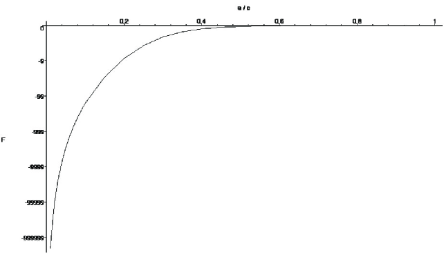
Figure 2: Casimir force $F$ versus $a/c$ for the case $b/c=1$ where $a$ is the plate separation and $b$ and $c$ are the sides of the base. The force is in units of $1/c^{2}$. The force is large and negative at small values of $a/c$ and remains negative with its magnitude decreasing quickly to zero as $a/c$ increases. One obtains a similar plot for any value of $b/c$ (see the 3D plot below)

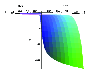
Figure 3: 3D plot of Casimir force $F$ versus $a/c$ and $b/c$. The force is in units of $1/c^{2}$. For a given $b/c$, the profile is the same as in the 2D plot: the force is large and negative at small values of $a/c$ and remains negative with its magnitude decreasing quickly to zero as $a/c$ increases. The value of $b/c$ shifts the magnitude of the force towards larger values as it increases.

A plot of the Casimir force $F$ versus $a/c$ is shown in Fig. 2 for the case $b/c=1$ (the force is in units of $1/c^{2}$). The Casimir force is negative, has a large magnitude at small values of $a/c$ and decreases rapidly in magnitude towards zero as $a/c$ increases in agreement with the two limits given by (2.18). One obtains a similar plot for any value of $b/c$. A 3D plot of $F$ versus $a/c$ and $b/c$ is shown in Fig. 3. The Casimir force is negative throughout and a slice taken at any value of $b/c$ yields a similar profile to the 2D plot in Fig.2 with the magnitude of the force shifting to greater values as $b/c$ increases. For any given slice, the Casimir force lies between the two limits given by (2.18).

Appendix A Explicit expression for Dirichlet Casimir energy for $d$-dimensional box with sides of arbitrary lengths

In this appendix, we derive the explicit formula (2.1) for the Casimir energy of massless scalar fields confined to a $d$-dimensional box of arbitrary lengths for Dirichlet boundary conditions. We begin by stating explicit formulas for the $d$-dimensional Casimir energy obeying periodic boundary conditions [18]. The second step is to express the Dirichlet energy as a sum over the periodic energy [18, 23] . The third step, the main part of the appendix, is to perform explicitly this sum to obtain the compact expression (A.12) for the Dirichlet energy.

The Casimir energy for massless scalar fields in a $d$-dimensional box of arbitrary lengths $L_{1},...,L_{d}$ and periodic boundary conditions can be explicitly expressed as an analytical part – composed of Riemann zeta and gamma functions – plus a sum of over Bessel functions [18]:

$$\begin{split}&E_{p_{{}_{\,L_{1},..,L_{d}}}}\,(d)=-\,\pi\sum_{j=0}^{d-1}\dfrac{L_{1}\ldots L_{j}}{(L_{j+1})^{j+1}}\Big{(}\Gamma(\tfrac{j+2}{2})\,\pi^{\frac{-j-4}{2}}\,\zeta(j+2)+R_{j}\Big{)}\\ &=\,\dfrac{-\pi}{6\,L_{1}}-\dfrac{\zeta(3)}{2\,\pi}\dfrac{L_{1}}{L_{2}^{2}}-\dfrac{\pi^{2}}{90}\dfrac{L_{1}\,L_{2}}{L_{3}^{3}}+\cdots-R_{1}\,\dfrac{\pi\,L_{1}}{L_{2}^{2}}-R_{2}\,\dfrac{\pi\,L_{1}\,L_{2}}{L_{3}^{3}}+\cdots\end{split}$$ (A.1)

where $R_{j}$ represents the sum over modified Bessel functions $K_{\nu}$:

$$R_{j}=\sum_{n=1}^{\infty}\,\sideset{}{{}^{\prime}}{\sum}_{\begin{subarray}{c}l_{i}=-\infty\\ i=1,\ldots,j\end{subarray}}^{\infty}\dfrac{2\,\,n^{\frac{j+1}{2}}}{\pi}\,\dfrac{\,K_{\frac{j+1}{2}}\big{(}\,2\pi\,n\,\sqrt{(\ell_{1}\frac{L_{1}}{L_{j+1}})^{2}+\cdots+(\ell_{j}\,\frac{L_{j}}{L_{j+1}})^{2}}\,\,\,\big{)}}{\left[(\ell_{1}\frac{L_{1}}{L_{j+1}})^{2}+\cdots+(\ell_{j}\frac{L_{j}}{L_{j+1}})^{2}\right]^{\tfrac{j+1}{4}}}\,\,.$$ (A.2)

The prime in the above sum means that the case where all $\ell$’s are zero is excluded. Note that for $j\!=\!0$ one sets $R_{j}$ to zero and $L_{j}$ identically to one so that $\frac{L_{1}\ldots L_{j}}{(L_{j+1})^{j+1}}$ is equal to $1/L_{1}$ for $j=0$. Note also that $R_{j}$ is a function of ratios of lengths i.e. $R_{j}=R_{j}(L_{1}/L_{j+1},...,L_{j}/L_{j+1})$. The notation $E_{p_{{}_{\,L_{1},\ldots,L_{d}}}}\,(d)$ is a compact way of saying that the Casimir energy $E_{p}$ is a function of the dimension $d$ and the lengths $L_{1},...,L_{d}$.

Our goal is to obtain a similar explicit expression for the case of Dirichlet boundary conditions. We begin by noting that the Dirichlet case can be expressed as a sum over the periodic Casimir energies $E_{p}$ (see [18, 23]):

$$E_{D}=\dfrac{1}{2^{d+1}}\sum_{m=1}^{d}\,(-1)^{d+m}\!\!\!\!\!\!\sum_{\begin{subarray}{c}\{k_{1},..,k_{m}\}\\ k_{1}<k_{2}<\cdots<k_{m}\\ \ k_{m}\leq d\end{subarray}}E_{p_{{}_{\,L_{k_{1}},..,L_{k_{m}}}}}(m)\,.$$ (A.3)

The sum over the $k_{i}$’s is over all sets $\{k_{1},..,k_{m}\}$, where the $k_{i}$ are integers that can run from $1$ to a maximum value of $d$ under the constraint that $k_{1}\!<\!k_{2}\!<\!\cdots\!<k_{m}$. To specify that $d$ is the maximum value we write $k_{m}\leq d$ under the sum in (A.3). $E_{p_{{}_{L_{k_{1}},..,L_{k_{m}}}}}(m)$ is the periodic energy (A.1) replacing $d$ by $m$ and $L_{1}$ by $L_{k_{1}}$, $L_{2}$ by $L_{k_{2}}$, etc. Note that the replacement $L_{1}$ by $L_{k_{1}}$, etc. must also be performed inside $R_{j}$ given by (A.2). The above notation for the sum over $k_{i}$ is cumbersome. It is convenient to introduce a symbol $\xi^{\,d}_{\,k_{1},..,k_{m}}$ defined by

$$\xi^{\,d}_{\,k_{1},..,k_{m}}=\begin{cases}1&\,\,\mbox{if}\,\,k_{1}\!<\!k_{2}\!<\!\ldots\!<k_{m}\,;\,1\leq k_{i}\leq d\\ 0&\,\,\mbox{otherwise}\,\,.\end{cases}$$ (A.4)

The superscript $d$ specifies the dimension which is the maximum value of $k_{m}$. The above defined symbol apparently does not have a name and for simplicity we shall refer to it as the $ordered$ symbol. Equation (A.3) can now be conveniently expressed with the $ordered$ symbol:

$$E_{D}=\dfrac{1}{2^{d+1}}\sum_{m=1}^{d}\,(-1)^{d\!+\!m}\,\xi^{\,d}_{\,k_{1},..,k_{m}}\,E_{p_{{}_{\,L_{k_{1}},..,L_{k_{m}}}}}(m)\,$$ (A.5)

where $implicit$ $summation$ over the $k_{i}$’s is assumed. After substituting (A.1) into (A.5) one obtains

$$E_{D}=\dfrac{-\pi}{2^{d+1}}\sum_{m=1}^{d}\,(-1)^{d+m}\xi^{\,d}_{\,k_{1},..,k_{m}}\,\Big{\{}\sum_{j=0}^{m-1}\dfrac{L_{k_{1}}\ldots L_{k_{j}}}{(L_{k_{j+1}})^{j+1}}\Big{(}\Gamma(\tfrac{j+2}{2})\,\pi^{\frac{-j-4}{2}}\,\zeta(j+2)+R_{j}\Big{)}\Big{\}}$$ (A.6)

where $R_{j}$ is the function (A.2) with $L_{1}$ replaced by $L_{k_{1}}$, $L_{2}$ by $L_{k_{2}}$, etc. For simplicity we define

$$f_{j_{{}_{\,\,k_{1},..,k_{j+1}}}}\equiv\dfrac{L_{k_{1}}\ldots L_{k_{j}}}{(L_{k_{j+1}})^{j+1}}\Big{(}\Gamma(\tfrac{j+2}{2})\,\pi^{\frac{-j-4}{2}}\,\zeta(j+2)+R_{j}\Big{)}$$ (A.7)

and rewrite (A.6) as

$$E_{D}=\dfrac{-\pi}{2^{d+1}}\sum_{m=1}^{d}\sum_{j=0}^{m-1}(-1)^{d+m}\,\xi^{\,d}_{\,k_{1},..,k_{m}}f_{j_{{}_{\,\,k_{1},..,k_{j+1}}}}\!\!\!\!=\dfrac{\pi}{2^{d+1}}\sum_{j=0}^{d-1}\sum_{m=j+1}^{d}(-1)^{d+m+1}\,\xi^{\,d}_{\,k_{1},..,k_{m}}f_{j_{{}_{\,\,k_{1},..,k_{j+1}}}}$$ (A.8)

where we have rewritten the limits on each sum. We can decompose $\xi^{\,d}_{\,k_{1},..,k_{m}}$ into a sum of two terms: $\xi^{\,d-1}_{\,k_{1},..,k_{m-1},d}+\xi^{\,d-1}_{\,k_{1},..,k_{m}}$. The first term, $\xi^{\,d-1}_{\,k_{1},..,k_{m-1},d}\,\,$, means that $k_{m}$ is set to its maximum value of $d$ and the sum is now over the remaining $k_{i}$’s with $k_{m-1}$ having a maximum possible value of $d-1$. With $k_{m}=d$ in the first term, the maximum possible value of $k_{m}$ in the second term is $d-1$ (hence the superscript $d-1$ in the second term). Note that for the special case $m=d$, the above decomposition yields only one term not two terms i.e. $\xi^{\,d}_{\,k_{1},..,k_{d}}=\xi^{\,d-1}_{\,k_{1},..,k_{d-1},d}+0$ since $k_{d}$ can only be equal to $d$.

With this decomposition the sum over $m$ becomes

$$\begin{split}&\sum_{m=j+1}^{d}(-1)^{d+m+1}\,\,\xi^{\,d}_{\,k_{1},..,k_{m}}=\sum_{m=j+1}^{d}(-1)^{d+m+1}\,\,\big{[}\,\xi^{\,d-1}_{\,k_{1},..,k_{m-1},d}+\xi^{\,d-1}_{\,k_{1},..,k_{m}}\,\big{]}\\ &=(-1)^{d+j}\big{[}\,\xi^{\,d-1}_{\,k_{1},..,k_{j},d}+(\,\xi^{\,d-1}_{\,k_{1},..,k_{j+1}}-\xi^{\,d-1}_{\,k_{1},..,k_{j+1},d}\,)-(\,\xi^{\,d-1}_{\,k_{1},..,k_{j+2}}-\xi^{\,d-1}_{\,k_{1},..,k_{j+2},d}\,)\\ &\quad\quad+\ldots(-1)^{d-j}(\,\xi^{\,d-1}_{\,k_{1},..,k_{d-1}}-\xi^{\,d-1}_{\,k_{1},..,k_{d-1},d})\,\big{]}\,.\end{split}$$ (A.9)

The two terms inside each pair of round brackets in (A.9) have opposite signs and cancel each other so that the sum over $m$ reduces to only the first term

$$\sum_{m=j+1}^{d}(-1)^{d+m+1}\,\,\xi^{\,d}_{\,k_{1},..,k_{m}}=(-1)^{d+j}\,\xi^{\,d-1}_{\,k_{1},..,k_{j},d}\,.$$ (A.10)

The Dirichlet Casimir energy is obtained by substituting (A.10) in (A.8):

$$E_{D}=\dfrac{\pi}{2^{d+1}}\!\sum_{j=0}^{d-1}(-1)^{d+j}\,\xi^{\,d-1}_{\,k_{1},..,k_{j},d}\,f_{j_{{}_{\,\,k_{1},..,k_{j+1}}}}\!\!\!\!=\!\dfrac{\pi}{2^{d+1}}\sum_{j=0}^{d-1}(-1)^{d+j}\,\xi^{\,d-1}_{\,k_{1},..,k_{j}}\,f_{j_{{}_{\,\,k_{1},\,..,\,k_{j},\,d}}}\,.$$ (A.11)

The function $f_{j_{{}_{\,\,k_{1},\,..,\,k_{j},\,d}}}$ is obtained by setting $k_{j+1}$ equal to $d$ in (A.7). We finally obtain our explicit expression for the Dirichlet Casimir energy

$$E_{D}=\dfrac{\pi}{2^{d+1}}\sum_{j=0}^{d-1}(-1)^{d+j}\,\,\xi^{\,d-1}_{\,k_{1},..,k_{j}}\,\Big{\{}\dfrac{L_{k_{1}}\ldots L_{k_{j}}}{(L_{d})^{j+1}}\Big{(}\Gamma(\tfrac{j+2}{2})\,\pi^{\frac{-j-4}{2}}\,\zeta(j+2)+R_{j}\Big{)}\,\Big{\}}$$ (A.12)

where $R_{j}$ is given by (A.2) with $L_{1}\to L_{k_{1}}$, $L_{j+1}\to L_{k_{j+1}}=L_{d}$ i.e.

$$R_{j}=\sum_{n=1}^{\infty}\,\sideset{}{{}^{\prime}}{\sum}_{\begin{subarray}{c}l_{i}=-\infty\\ i=1,\ldots,j\end{subarray}}^{\infty}\dfrac{2\,\,n^{\frac{j+1}{2}}}{\pi}\,\dfrac{\,K_{\frac{j+1}{2}}\big{(}\,2\pi\,n\,\sqrt{(\ell_{1}\frac{L_{k_{1}}}{L_{d}})^{2}+\cdots+(\ell_{j}\,\frac{L_{k_{j}}}{L_{d}})^{2}}\,\,\,\big{)}}{\left[(\ell_{1}\frac{L_{k_{1}}}{L_{d}})^{2}+\cdots+(\ell_{j}\frac{L_{k_{j}}}{L_{d}})^{2}\right]^{\tfrac{j+1}{4}}}\,\,.$$ (A.13)

For the case $j=0$, $R_{j}$ is zero and $\xi^{\,d-1}_{\,k_{1},..,k_{j}}$ and $L_{k_{j}}$ are defined as unity.

Appendix B Alternative expression for Casimir force on piston

One can derive an alternative expression for the Casimir force $F$ on the piston by labeling the lengths $L_{1}$, $L_{2}$ and $L_{3}$ differently. We are free to label the lengths in any way we want since the Casimir energy is invariant under permutations of $L_{1}$, $L_{2}$ and $L_{3}$. In region I, the three lengths are $a$, $b$ and $c$ and we label them now $L_{1}=a$, $L_{2}=c$ and $L_{3}=b$. In region II, the three lengths are $s-a$, $b$ and $c$ and we label them now $L_{1}=s-a$, $L_{2}=c$ and $L_{3}=b$. The Dirichlet Casimir energy in region I and II is then obtained via (2.4)

$$\begin{split}E_{D1}&=-\dfrac{\pi^{2}}{1440}\,\dfrac{a\,c}{b^{3}}+\dfrac{\zeta(3)}{32\,\pi\,b^{2}}(a+c)-\dfrac{\pi}{96\,b}+R(a,c,b)\\ E_{D2}&=-\dfrac{\pi^{2}}{1440}\,\dfrac{(s-a)\,c}{b^{3}}+\dfrac{\zeta(3)}{32\,\pi\,b^{2}}(s-a+c)-\dfrac{\pi}{96\,b}+R(s-a,c,b)\end{split}$$ (B.1)

where $R(a,c,b)$ and $R(s-a,c,b)$ are defined via (2.5) and (2.6). The Casimir force $F_{1}$ due to region I and $F_{2}$ due to region II (with $s\to\infty$) are

$$\begin{split}F_{1}&=-\dfrac{\partial}{\partial\,a}E_{D1}=\dfrac{\pi^{2}}{1440}\,\dfrac{c}{b^{3}}-\dfrac{\zeta(3)}{32\,\pi\,b^{2}}-R^{\prime}(a,c,b)\\ F_{2}&=\lim_{s\to\infty}-\dfrac{\partial}{\partial\,a}E_{D2}=-\dfrac{\pi^{2}}{1440}\,\dfrac{c}{b^{3}}+\dfrac{\zeta(3)}{32\,\pi\,b^{2}}-\lim_{s\to\infty}R^{\prime}(s-a,c,b)\,.\end{split}$$ (B.2)

The total Casimir force $F=F_{1}+F_{2}$ on the piston is then simply

$$F=-R^{\prime}(a,c,b)-\lim_{s\to\infty}R^{\prime}(s-a,c,b)$$ (B.3)

where the prime denotes derivative with respect to the plate separation $a$. Note that the analytical terms – the Riemann zeta and gamma terms – have canceled. This is also what occurs in the two-dimensional Casimir piston (see [1]). The second term in (B.3) has already been obtained and is given by (2.12). The function $R(a,c,b)$ can be obtained from the function $R(c,b,a)$ given by (2.8) by replacing $c$ with $a$, $b$ with $c$ and $a$ with $b$ i.e.

$$\begin{split}R(a,c,b)&=\dfrac{1}{4\,b}\sum_{n=1}^{\infty}\sum_{\ell=1}^{\infty}\,\dfrac{n}{\ell}\,\Big{[}K_{1}\big{(}2\,\pi\,n\,\ell\,a/b\big{)}+K_{1}\big{(}2\,\pi\,n\,\ell\,c/b\big{)}\Big{]}\\ &\qquad\qquad-\dfrac{\,a\,c}{8\,b^{3}}\,\sum_{n=1}^{\infty}\,\sideset{}{{}^{\prime}}{\sum}_{\ell_{1},\ell_{2}=-\infty}^{\infty}\!\!\dfrac{n^{3/2}\,K_{3/2}\Big{(}2\,\pi\,n\,\sqrt{\Big{(}\dfrac{\ell_{1}\,a}{b}\Big{)}^{2}+\Big{(}\dfrac{\ell_{2}\,c}{b}\Big{)}^{2}}\,\,\Big{)}}{\left[\Big{(}\dfrac{\ell_{1}\,a}{b}\Big{)}^{2}+\Big{(}\dfrac{\ell_{2}\,c}{b}\Big{)}^{2}\right]^{3/4}}\,.\end{split}$$ (B.4)

The derivative of $R(a,c,b)$ with respect to the plate separation $a$ is

$$\begin{split}R^{\prime}(a,c,b)&=\dfrac{1}{4\,b}\sum_{n=1}^{\infty}\sum_{\ell=1}^{\infty}\,\dfrac{n}{\ell}\,K_{1}^{\prime}\big{(}2\,\pi\,n\,\ell\,a/b\big{)}\\ &-\dfrac{\partial}{\partial\,a}\,\Bigg{[}\dfrac{a\,c}{8\,b^{3}}\,\sum_{n=1}^{\infty}\,\sideset{}{{}^{\prime}}{\sum}_{\ell_{1},\ell_{2}=-\infty}^{\infty}\!\!\dfrac{n^{3/2}\,K_{3/2}\Big{(}2\,\pi\,n\,\sqrt{\Big{(}\dfrac{\ell_{1}\,a}{b}\Big{)}^{2}+\Big{(}\dfrac{\ell_{2}\,c}{b}\Big{)}^{2}}\,\,\Big{)}}{\left[\Big{(}\dfrac{\ell_{1}\,a}{b}\Big{)}^{2}+\Big{(}\dfrac{\ell_{2}\,c}{b}\Big{)}^{2}\right]^{3/4}}\Bigg{]}\,.\end{split}$$ (B.5)

With $R^{\prime}(a,c,b)$ given by (B.5) and $\lim_{s\to\infty}R^{\prime}(s-a,c,b)$ given by (2.12), the Casimir force (B.3) yields

$$\begin{split}F&=-\dfrac{1}{4\,b}\sum_{n=1}^{\infty}\sum_{\ell=1}^{\infty}\,\dfrac{n}{\ell}\,K_{1}^{\prime}\big{(}2\,\pi\,n\,\ell\,a/b\big{)}\\ &+\dfrac{\partial}{\partial\,a}\,\Bigg{[}\dfrac{a\,c}{8\,b^{3}}\,\sum_{n=1}^{\infty}\,\sideset{}{{}^{\prime}}{\sum}_{\ell_{1},\ell_{2}=-\infty}^{\infty}\!\!\dfrac{n^{3/2}\,K_{3/2}\Big{(}2\,\pi\,n\,\sqrt{\Big{(}\dfrac{\ell_{1}\,a}{b}\Big{)}^{2}+\Big{(}\dfrac{\ell_{2}\,c}{b}\Big{)}^{2}}\,\,\Big{)}}{\left[\Big{(}\dfrac{\ell_{1}\,a}{b}\Big{)}^{2}+\Big{(}\dfrac{\ell_{2}\,c}{b}\Big{)}^{2}\right]^{3/4}}\Bigg{]}\\ &-\dfrac{c}{4\,b^{3}}\,\sum_{n=1}^{\infty}\,\sum_{\ell_{2}=1}^{\infty}\dfrac{n^{3/2}\,K_{3/2}\Big{(}2\,\pi\,n\,\ell_{2}\,c/b\Big{)}}{\Big{(}\dfrac{\ell_{2}\,c}{b}\Big{)}^{3/2}}\,.\end{split}$$ (B.6)

The above expression has three terms and it can be simplified by noticing that the $\ell_{1}=0$ case in the second term cancels out with the last term. The Casimir force on the piston reduces to the following final expression:

$$\begin{split}F_{alt}&=-\dfrac{1}{4\,b}\sum_{n=1}^{\infty}\sum_{\ell=1}^{\infty}\,\dfrac{n}{\ell}\,K_{1}^{\prime}\big{(}2\,\pi\,n\,\ell\,a/b\big{)}\\ &+\dfrac{\partial}{\partial\,a}\,\Bigg{[}\dfrac{a\,c}{4\,b^{3}}\,\sum_{n=1}^{\infty}\,\sum_{\ell_{1}=1}^{\infty}\sum_{\ell_{2}=-\infty}^{\infty}\!\!\dfrac{n^{3/2}\,K_{3/2}\Big{(}2\,\pi\,n\,\sqrt{\Big{(}\dfrac{\ell_{1}\,a}{b}\Big{)}^{2}+\Big{(}\dfrac{\ell_{2}\,c}{b}\Big{)}^{2}}\,\,\Big{)}}{\left[\Big{(}\dfrac{\ell_{1}\,a}{b}\Big{)}^{2}+\Big{(}\dfrac{\ell_{2}\,c}{b}\Big{)}^{2}\right]^{3/4}}\Bigg{]}\,.\end{split}$$ (B.7)

The above is our alternative expression for the Casimir force on the piston. It is valid for any positive values of $a$, $b$ and $c$ but it is especially useful computationally when $a$ is not the smallest of the three lengths. We are free to label the base such that $c\geq b$. If $a$ is not the smallest length, then the ratios $a/b$ and $c/b$ are both greater than or equal to one. This ensures that the sums over the Bessel functions and their derivatives in (B.7) will converge exponentially fast making computations easy and accurate. Note that the sum over $\ell_{1}$ and the sum over $\ell$ in (B.7) do not include zero. Therefore as $a$ increases the Bessel functions and their derivatives will always decrease exponentially and reach zero in the limit $a\to\infty$. The Casimir force on the piston is therefore zero in the limit $a\to\infty$.