TPJU-13/2006

Solving some gauge systems at infinite N

J. Wosiek

M. Smoluchowski Institute of Physics, Jagellonian University

Reymonta 4, 30-059 Kraków, Poland

Abstract

After summarizing briefly some numerical results for four-dimensional supersymmetric SU(2) Yang-Mills quantum mechanics, we review a recent study of systems with an infinite number of colours. We study in detail a particular supersymmetric matrix model which exhibits a phase transition, strong-weak duality, and a rich structure of supersymmetric vacua. In the planar and strong coupling limits, this field theoretical system is equivalent to a one-dimensional XXZ Heisenberg chain and, at the same time, to a gas of $q$-bosons. This not only reveals a hidden supersymmetry in these well-studied models; it also maps the intricate pattern of our supersymmetic vacua into that of the now-popular ground states of the XXZ chain.

TPJU-13/2006

October 2006

1 Introduction

This lecture reviews a recent progress in studying the large N limit of simple supersymmetric quantum mechanical systems which result from the dimensional reduction of field theories with gauge symmetry. Models of this type have been studied for a long time [1, 2, 3] and have many different applications, depending on the space-time dimension, D, of the unreduced theory [4, 5] (cf. Table 1). For D=2 they can be often solved analytically [1, 4, 6, 7], providing quantitative realization of supersymmetry. In four space-time dimensions one of them is nothing but the small volume limit of the Yang-Mills gluodynamics revealing the spectrum of zero volume glueballas as a special case [8, 9, 10, 11]. Finally, for D=10 they make contact with the M-theory via the BFSS hypothesis [12].

$D$	$2$	$4$	$\dots$	$10$
$N$
2	$\bullet$	$\bullet$		$\circ$
3	$\bullet$
.	$\circ$
.	$\circ$
.
$\infty$	$\checkmark$			M

Table 1: A ”road map” of a parameter space of supersymmetric Yang-Mills quantum mechanics. Black dots denote models well understood/solved, while open circles mark ones under study. A checkmark labels parameters of a system discussed in this lecture.

Although we shall be mainly concerned with the large N limit, we would like to give one example of the N=2 model.

1.1 Four-dimensional supersymmetric Yang-Mills quantum mechanics at finite N

The system has three bosons and two fermions, both in the adjoint representation of SU(2). The Hamiltonian reads [1]

$$H = {1\over 2}p_{a}^{i}p_{a}^{i}+{g^{2}\over 4}\epsilon_{abc}\epsilon_{ade}x_{b}^{i}x_{c}^{j}x_{d}^{i}x_{e}^{j}+{ig\over 2}\epsilon_{abc}\psi_{a}^{\dagger}\Gamma^{k}\psi_{b}x_{c}^{k},$$

$$i=1,2,3 a=1,2,3.$$

The spectrum is obtained numerically by diagonalizing $H$ in the gauge invariant eigen-basis of the occupation numbers of all degrees of freedom $n_{a}^{i}={a^{\dagger}}_{a}^{i}a_{a}^{i},\eta_{a}^{i}={f^{\dagger}}_{a}^{i}f_{a}^{i}$ [3]

$$|\{n_{a}^{i},\eta_{c}^{j}\}>=\sum_{contractions}{a^{\dagger}}^{i}_{c}{{a^{\dagger}}}^{j}_{d}{a^{\dagger}}^{k}_{e}{f^{\dagger}}_{b}^{m}{f^{\dagger}}_{a}^{n}\dots|0>.$$

The Hilbert space was cut by restricting the gauge invariant total number of bosonic quanta

$$B=\sum_{b,i}{a^{\dagger}}_{b}^{i}a_{b}^{i}<B_{max}.$$

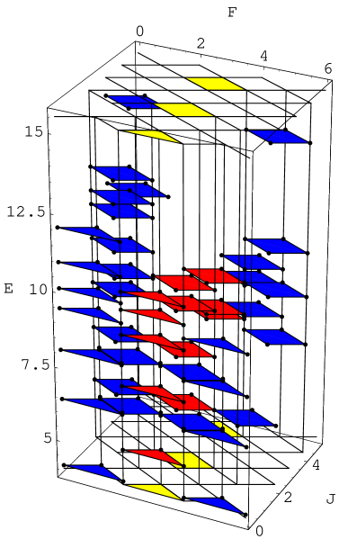
Figure 1: The spectrum, and its supersymmetry structure, of the D=4 supersymmetric Yang-Mills quantum mechanics.

It turned out that the physical (i.e. convergent with the cutoff eigenenergies) could be computed for sizes of bases well within a reach of a reasonably fast PC. The spectrum obtained in this way is shown in Fig. 1 [5]. It reveals a series of dynamical supermultiplets with degenerate eigenenergies. The eigenstates within a supermultiplet are indeed the supersymmetric images of one another. These states are localized and they form a discrete spectrum. In addition there is also a continuum. It occupies central sectors of the figure, i.e. ones with the conserved fermion number $F=2,3,4$. Supermultiplets of non-localized states occur at every second value of the angular momentum. Moreover, in these sectors the discrete and continuous spectra coexists at the same energies. This unusual feature of gauge interactions has never been observed so directly before. There are two supersymmetric vacua with fermion numbers $F=2$ and $4$. This is nothing but the zero-volume manifestation of the existence of the $\lambda\lambda$ condensate in the space extended theories [13]. The condensate assumes two different (in fact opposite for SU(2)) values, again in agreement with the non-trivial predictions of the unreduced theory [14, 15] .

2 The large N limit and the planar calculus

Above approach, even though quite successful, is naturally limited to the low number of colours. For higher N the Hilbert spaces become too large. Fortunately at infinite N Fock bases simplify enormously allowing again to reach quantitative results [16]-[20]. This simplification is usually phrased in terms of the Feynman diagrams and topological expansion [21]. However it can be also formulated in the way suitable for the Hamiltonian formalism [16, 17]. To this end introduce matrix creation and annihilation (c/a) operators.

$$a_{ik}=\sqrt{2}a^{a}T^{a}_{ik},\;\;\;f_{ik}=\sqrt{2}f^{a}T^{a}_{ik},\;\;\;i,k=1,...,N.$$

The physical basis can be conveniently generated by acting with the gauge invariant building blocks (bricks)

$$({a^{\dagger}}{a^{\dagger}}),({a^{\dagger}}{a^{\dagger}}{a^{\dagger}}),({a^{\dagger}}{a^{\dagger}}{a^{\dagger}}{a^{\dagger}}),\dots,({a^{\dagger}}^{N}),\;\;\;(.)\equiv Tr[.]$$

and their products, on the empty Fock state $|0\rangle$. Similarly for the fermionic sectors one employs bricks with mixed fermionic and bosonic operators. It turns out that in the large N limit only the single trace operators are relevant. All products of traces are either non-leading or do not provide new information (see [22] for recent results on that point). This observation culminates in the set of simple rules to calculate explicitly matrix elements of various Hamiltonians. One basically applies the Wick theorem employing the commutation rules

$$[a_{ik},{a^{\dagger}}_{jl}]=\delta_{il}\delta_{kj}$$

and identifying the leading contributions. Details of such ”planar calculus” have been presented in [16, 17, 19]. Here we summarize only two examples

A normalized state with n gluons in the F=0 sector reads

$$|n>=\frac{1}{{\cal N}_{n}}Tr[({a^{\dagger}})^{n}]|0>.$$ (1)

The normalization factor

$${\cal N}_{n}^{2} = <0|Tr[a^{n}]Tr[({a^{\dagger}})^{n}]|0>$$

$$= <0|(12)(23)...(n1)[1^{\prime}2^{\prime}][2^{\prime}3^{\prime}]\dots[n^{\prime}1^{\prime}]|0>,$$

$$(12)\equiv a_{i_{1}i_{2}}, [12]\equiv{a^{\dagger}}_{i_{1}i_{2}}.$$

receives the maximal contribution only when the adjacent creation and annihilation operators are contracted. This gives

$${\cal N}_{n}^{2}=nN^{n}.$$

Similarly a matrix element of a typical term in a generic Hamiltonian

$$H_{n+2,n}=g^{2}<n+2|Tr[{a^{\dagger}}{a^{\dagger}}{a^{\dagger}}a]|n>$$

can be explicitly calculated

$$H_{n+2,n}=g^{2}N\sqrt{n(n+2)},$$

and shown to depend only on the ’t Hooft coupling $\lambda=g^{2}N$.

The rest of this lecture will be devoted to a rather simple system which turns out to be surprisingly rich. The model may be considered as a distant cousin of the $D=1+1$ supersymmetric Yang-Mills theory reduced to the one point in space.

3 A simple supersymmetric system

Consider one fermion and one boson with the following supersymmerty generators and the Hamiltonian [16].

$$Q=\sqrt{2}Tr[f{a^{\dagger}}(1+g{a^{\dagger}})], {Q^{\dagger}}=\sqrt{2}Tr[{f^{\dagger}}(1+ga)a],$$

$$H= \{Q,{Q^{\dagger}}\} =H_{B}+H_{F}.$$ (2)

Explicitly

$$H_{B} = {a^{\dagger}}a+g({a^{\dagger}}^{2}a+{a^{\dagger}}a^{2})+g^{2}{a^{\dagger}}^{2}a^{2},$$

$$H_{F} = {f^{\dagger}}f+g({f^{\dagger}}f({a^{\dagger}}+a)+{f^{\dagger}}({a^{\dagger}}+a)f)$$

$$+ g^{2}({f^{\dagger}}af{a^{\dagger}}+{f^{\dagger}}a{a^{\dagger}}f+{f^{\dagger}}f{a^{\dagger}}a+{f^{\dagger}}{a^{\dagger}}fa).$$

This Hamiltonian conserves the gauge invariant fermion number $F=Tr[{f^{\dagger}}f]$ and can be diagonalized in sectors with well defined $F$. For any finite N calculation of matrix elements of H quickly becomes cumbersome. At infinite N, however, the planar rules illustrated above give simple and compact expressions.

3.1 Hamiltonian matrix at large N

The gauge invariant basis in the $F=0$ sector can be chosen as (1) with $n=0,1,2,3,...$. Only $H_{B}$ contributes in this case. The matrix elements in the planar approximation read

$$<0,n|H|0,n> = (1+\lambda(1-\delta_{n1}))n,$$

$$<0,n+1|H|0,n>= <0,n|H|0,n+1>= \sqrt{\lambda}\sqrt{n(n+1)}.$$ (3)

In the sector with one fermion the basis is

$$|n>=\frac{1}{{\cal N}_{n}}Tr[({f^{\dagger}}{a^{\dagger}})^{n}]|0>,\;\;\;n=0,1,2,\dots.$$

Now, and for higher $F$, both $H_{B}$ and $H_{F}$ contribute. The Hamiltonian matrix is again simple

$$<1,n|H|1,n> = (1+\lambda)(n+1)+\lambda,$$

$$<1,n+1|H|1,n>= <1,n|H_{2}|1,n+1>= \sqrt{\lambda}(2+n).$$ (4)

The system reveals many interesting features already in these two lower sectors [16], therefore we postpone the discussion of higher F’s and turn to the physics of ensembles with at most one fermion.

3.2 Numerical results

The Hamiltonian matrix is sparse but infinite with rows and columns labeled by the gauge invariant number of bosons $B=Tr[{a^{\dagger}}a]$. To obtain, the spectrum numerically we introduce the cutoff, $B_{max}$, limiting the number of bosonic quanta

$$B<B_{max},$$

and increase the cutoff until the spectrum converges. Results are shown in Fig.2 for few values of the ’t Hooft coupling. The convergence with $B_{max}$ is satisfactory for $\lambda\neq 1$ and is faster for lower eigenvalues. There, the limiting, ”infinite volume”, results can be easily recovered. The less trivial way so see this is to check for the supersymmetry which is broken by the cutoff and should be recovered only at infinite $B_{max}$. Figure 3 shows first few energy levels in four lower fermionic sectors. The degeneracies between bosonic and fermionic partners of the $F=(0,1)$ supermultiplets are excellent. Moreover, there is also an unbalanced supersymmetric vacuum state with zero eigenenergy . These results provide also the non-trivial test of our planar rules: the planar approximation does not break supersymmetry.

The slowing of the cutoff dependence around $\lambda=1$ is a characteristic signature of a phase transition. At this point the system looses the energy gap and the spectrum becomes continuous. Any finite number of low-lying levels collapses to zero at infinite cutoff, but the cutoff dependence becomes characteristic of that for the continuous spectrum.

Figure 2: The cutoff dependence of the spectra of $H$ in the F=0 sector, and for a range of $\lambda$’s

Another interesting feature of this phase transition is the rearrangement of members of supermultiplets. This is shown in Fig.4 where the $\lambda$ dependence of the first four eigenenergies from both sectors is displayed for few values of $B_{max}$. Away from the critical region supersymmetry is quickly restored and the F=0 and F=1 levels are undistinguishable even for low cutoffs. Close to the criticality partners do not have the same energies since SUSY is broken at finite cutoff. Interestingly however, they rearrange while the ’t Hooft coupling passes its critical value. In particular, the new vacuum state appears when $\lambda$ moves from the low to the large coupling phases. This also implies (and was readily found) that the Witten index (restricted to the $F=0,1$ sectors) jumps by one unit across the phase transition point.

Figure 3: Low lying bosonic and fermionic levels in the first four fermionic sectors.

Finally, the system has the exact strong-weak duality

$$b\left(E^{(F=0)}_{n}(1/b)-\frac{1}{b^{2}}\right) = \frac{1}{b}\left(E^{(F=0)}_{n+1}(b)-b^{2}\right),$$

$$b\left(E^{(F=1)}_{n}(1/b)-\frac{1}{b^{2}}\right) = \frac{1}{b}\left(E^{(F=1)}_{n}(b)-b^{2}\right).$$

It follows directly from the matrix representation (4) for $F=1$ . However it is not obvious in the $F=0$ sector, cf. Eq. (3), but it is a direct consequence of supersymmetry.

3.3 Analytic solution

All above results have been subsequently derived analytically [16]. For example the second vacuum state has the form $b\equiv\sqrt{\lambda}$

$$|0\rangle_{2}=\sum_{n=1}^{\infty}\left(\frac{-1}{b}\right)^{n}\frac{1}{\sqrt{n}}|0,n\rangle\ .$$ (5)

It is indeed annihilated by ${Q^{\dagger}}$, and exists only for $b>1$.

Surprisingly, one can find analytically the complete spectrum and construct all eigenstates in the $F=0$ sector. To this end it is convenient to introduce another, not orthonormal basis,

$$|B_{n}\rangle = \sqrt{n}|n\rangle+b\sqrt{n+1}|n+1\rangle\,.$$

Figure 4: Lowest bosonic and fermionic levels, as functions of $\lambda$, for different cutoffs

This basis is convenient since the action of the Hamiltonian on $|B_{n}\rangle$ is so simple that the generating function for the expansion of the eigenstates in that basis

$$f(x)=\sum_{n=0}^{\infty}c_{n}x^{n}\,\;\;\;\;\;\;\leftrightarrow\;\;\;\;\;\;|\psi\rangle=\sum_{n=0}^{\infty}c_{n}|B_{n}\rangle$$

can be constructed. The solution reads

$$f(x) = \frac{1}{\alpha}\;\frac{1}{x+1/b}\;F(1,\alpha;1+\alpha;\frac{x+b}{x+1/b}),\;\;\;b<1,$$

$$f(x) = \frac{1}{1-\alpha}\;\frac{1}{x+b}\;F(1,1-\alpha;2-\alpha;\frac{x+1/b}{x+b}),\;\;\;b>1,$$

$$E = \alpha(b^{2}-1),$$

and together with the quantization condition

$$f(0)=0,$$ (6)

reproduces numerical eigenvalues obtained earlier in the infinite cutoff limit.

As a one check, set $\alpha=0$ in the generating function, for $b>1$, to obtain

$$f_{0}(x)=\frac{1}{1+bx}\log\frac{b+x}{b-1/b},\;\;\;b>1,$$ (7)

which indeed reproduces the second ground state (5).

4 Higher fermionic sectors: F=2,3

Single trace states with two fermions

$$|n_{1},n_{2}\rangle = \frac{1}{{\cal N}_{n_{1}n_{2}}}Tr[{a^{\dagger}}^{n_{1}}{f^{\dagger}}{a^{\dagger}}^{n_{2}}{f^{\dagger}}]|0\rangle,$$

are labeled by two integers whose ordering is important modulo a cyclic permutation. Pauli principle eliminates states with $n_{1}=n_{2}$, hence we can always take $n_{2}<n_{1}$. The planar rules give for the Hamiltonian matrix in this sector [19]

$$\langle n_{1},n_{2}|H|n_{1},n_{2}\rangle = (n_{1}+n_{2}+2)(1+b^{2})-b^{2}(2-\delta_{n_{1},0})-2b^{2}\delta_{n_{2},n_{1}+1},$$

$$\langle n_{1}+1,n_{2}|H|n_{1},n_{2}\rangle= b(n_{1}+2) =\langle n_{1},n_{2}|H|n_{1}+1,n_{2}\rangle,$$

$$\langle n_{1},n_{2}+1|H|n_{1},n_{2}\rangle= b(n_{2}+2) =\langle n_{1},n_{2}|H|n_{1},n_{2}+1\rangle.$$

$$\langle n_{1}+1,n_{2}-1|H|n_{1},n_{2}\rangle = \langle n_{1},n_{2}|H|n_{1}+1,n_{2}-1\rangle$$

$$= 2b^{2}(1-\delta_{n_{2},n_{1}+1}).$$

Planar states in the three fermion sector are labeled by three integers modulo cyclic translations

$$|n_{1},n_{2},n_{3}\rangle = \frac{1}{{\cal N}_{n_{1}n_{2}n_{3}}}Tr[{a^{\dagger}}^{n_{1}}{f^{\dagger}}{a^{\dagger}}^{n_{2}}{f^{\dagger}}{a^{\dagger}}^{n_{3}}{f^{\dagger}}]|0\rangle,$$

$$0\leq n_{1},\;\;\;\; n_{1}\leq n_{2},\;\;\;\;\ n_{1}\leq n_{3}.$$

Again the Hamiltonian matrix was explicitly calculated

$$\langle n_{1},n_{2},n_{3}|H|n_{1},n_{2},n_{3}\rangle=(n_{1}+n_{2}+n_{3}+3)(1+b^{2})$$

$$-b^{2}(3-\delta_{n_{1},0}-\delta_{n_{2},0}-\delta_{n_{3},0}),$$

$$\langle n_{1}+1,n_{2},n_{3}|H|n_{1},n_{2},n_{3}\rangle =b(n_{1}+2)\Delta= \langle n_{1},n_{2},n_{3}|H|n_{1}+1,n_{2},n_{3}\rangle,$$

$${\rm plus~{}cyclic}$$

$$\langle n_{1}+1,n_{2}-1,n_{3}|H|n_{1},n_{2},n_{3}\rangle =b^{2}\Delta= \langle n_{1},n_{2},n_{3}|H|n_{1}+1,n_{2}-1,n_{3}\rangle,$$

$${\rm plus~{}cyclic}.$$

where $\Delta=1/\sqrt{3}$ if $n_{1}=n_{2}=n_{3}$, and $\Delta=\sqrt{3}$ if the final state is of this form, otherwise $\Delta=1$.

Numerical computation of the spectrum proceeds as before. There is again a phase transition causing the critical slowing down around $\lambda_{c}=1$. Away from it, the eigenenergies converge satisfactorily, with the infinite volume results shown in Fig.3. The spectrum in higher fermionic sectors is essentially different from the $F=0,1$ case. We again find dynamical $F=(2,3)$ supermultiplets, however not all states with three fermions have their superpartners in the $F=2$ sector. Instead, they are degenerate with ones from the $F=4$ sector. This pattern continues now for all F as follows from counting the number of states: it is an increasing function of F. Another novel feature is that the spectrum is rather irregular, while the eigenenergies are almost equidistant for $F=0,1$. There is again the rearrangement of members of supermultiplets across the phase transition. Interestingly however, the two new SUSY vacua with $F=2$ appear in the strong coupling phase, while there is none at weak coupling.

Similarly to the $F=0$ case, the two vacua can be constructed analytically. To this end consider the ”extreme” strong coupling limit of the Hamiltonian (2)[19]

$$H_{SC}=\lim_{\lambda\rightarrow\infty}\frac{1}{\lambda}H=Tr({f^{\dagger}}f)+\frac{1}{N}[Tr({a^{\dagger}}^{2}a^{2})+Tr({a^{\dagger}}{f^{\dagger}}af)+Tr({f^{\dagger}}{a^{\dagger}}fa)].$$ (8)

Surprisingly, $H_{SC}$ conserves the number of bosonic quanta as well, and proves very useful in mapping the structure of the model in all fermionic sectors (cf. the following Section). Coming back to $F=2$, one can identify the finite dimensional $(F=2,B)$ sectors with zero eigenvalues, and construct the corresponding eigenstates. They read

$$|F=2,v\rangle_{1}^{\infty} = |0,1\rangle,$$ (9)

$$|F=2,v\rangle_{2}^{\infty} = |0,3\rangle-2|1,2\rangle,$$ (10)

the superscript referring to the infinite value of the ’t Hooft coupling. These states can then be used to construct the two vacua at finite $\lambda>1$

$$|F=2,v\rangle_{1}^{\lambda} = \sum_{n=1}^{\infty}(-\sqrt{\lambda})^{-n}|0,n\rangle,\$$

$$|F=2,v\rangle_{2}^{\lambda} = (1+Q_{s}H_{s}^{-1}{Q^{\dagger}}_{w})^{-1}|F=2,v\rangle_{2}^{\infty},$$ (11)

with $Q_{s}=gTr[f{a^{\dagger}}^{2}],\;H_{s}=\{Q_{s},{Q^{\dagger}}_{s}\},\;{Q^{\dagger}}_{w}=Tr[{f^{\dagger}}a]$ [19].

The restoration of supersymmetry can also bee seen on the level of eigenstates. Members of supermultiplets transform among themselves by SUSY charges $Q$ and ${Q^{\dagger}}$, which become the well defined matrices in the planar bases. To see SUSY in this way define the following supersymmetry fractions

$$q_{mn}\equiv\sqrt{\frac{2}{E_{m}+E_{n}}}<F+1,E_{m}|Q^{\dagger}|F,E_{n}>,$$ (12)

which are the coordinates of the supersymmetric images of eigenstates in the corresponding fermionic sectors. Fig.5 shows that SUSY fractions indeed quickly stabilize with incrasing $B_{max}$.

Figure 5: First five supersymmetry fractions.

Supersymmtery fractions are also useful in defining the restricted Witten index which smoothly interpolates, at finite cutoff, between the two phases. The straightforward restriction of the sum

$$W(T,\lambda)=\sum_{i}(-1)^{F_{i}}e^{-TE_{i}},$$

to the $F=2,3$ eigenstates does not suffice since some of the states with three fermions remain unbalanced. Instead, one can define

$$W_{R}(T,\lambda)=\sum_{i}\left(e^{-TE_{i}}-e^{-T\bar{E}_{i}}\right),\;\;\;\bar{E}_{i}=\frac{\sum_{f}E_{f}|q_{fi}|^{2}}{\sum_{f}|q_{fi}|^{2}},$$

i.e. we take as the energy of the supersymmetric partner the energy weighted by supersymmetric fractions. This definition enforces summation only over complete supermultiplets away from the critical region, while provides the smooth smearing among possible candidates around $\lambda_{c}$. The index defined this way changes smoothly at finite cutoff, and varies by two units as expected (cf. Fig.6) [19].

Figure 6: Behaviour of the restricted Witten index, at $T=6$, around the phase transition.

5 Arbitrary F

A simple generalization of the $F=2,3$ cases for arbitrary number of fermions reads [18]

$$|n\rangle=|n_{1},n_{2},\dots,n_{F}\rangle=\frac{1}{{\cal N}_{\{n\}}}Tr({a^{\dagger}}^{n_{1}}{f^{\dagger}}{a^{\dagger}}^{n_{2}}{f^{\dagger}}\dots{a^{\dagger}}^{n_{F}}{f^{\dagger}})|0\rangle$$ (13)

So the states of the basis may be labeled by $F$ bosonic occupation numbers $\{n_{1},n_{2},\dots n_{F}\}$ (configurations) modulo cyclic shifts. Some states are excluded by the Pauli principle. For example

$$\{3,3\},\;\;\;\;\;{\rm or}\;\;\;\;\;\{2,1,1,1,2,1,1,1\}$$

are not allowed, since they change sign while retaining their identity after the suitable number of cyclic shifts. When calculating normalizations and matrix elements one should keep track of symmetry factors defined as the number of cyclic shifts which bring a state back to itself. For example the state $|2,1,2,1,2,1\rangle$ has the symmetry factor $d=3$. Alternatively one can label planar states with the periodic binary strings (necklaces) with, e.g., zeros/ones corresponding to the bosonic/fermionic creation operators (for a more complete discussion see [18]).

Detailed calculation of spectra for arbitrary fermion number is now in progress. However many properties, e.g. the supersymmetry structure, has been inferred from the strong coupling limit of the model.

As already mentioned, the strong coupling Hamltonian (8) conserves both fermionic and bosonic numbers of quanta. Hence the Hilbert space splits into the finite dimensional sectors, cf. Table 2, and the Hamiltonian in each sector becomes a finite matrix. Still the $H_{SC}$ has the exact supersymmetry with the strong-coupling charges

$$Q_{SC}=\frac{1}{\sqrt{N}}Tr[f{a^{\dagger}}^{2}],\;\;\;{Q^{\dagger}}_{SC}=\frac{1}{\sqrt{N}}Tr[f{a^{\dagger}}^{2}],$$ (14)

acting along the ”diagonals” $2F+B=const.$ of Table 2. Diagonalizing few of these matrices we have indeed found expected degeneracies. Interestingly, we have also found experimentally [18, 20] that the zero energy eigenstates are located only in the sectors with

$$B=F\pm 1,\;\;\;F\;even.$$ (15)

which form the regular ”magic” staircase, shown in the boldface, in Table 2.

$11\;\;\;$	1	1	6	26	91	273	728	1768	3978	8398	16796
$10\;\;\;$	1	1	5	22	73	201	497	1144	2438	4862	9226
$9\;\;\;$	1	1	5	19	55	143	335	715	1430	2704	4862
$8\;\;\;$	1	1	4	15	42	99	212	429	809	1430	2424
$7\;\;\;$	1	1	4	12	30	66	132	247	429	715	1144
$6\;\;\;$	1	1	3	10	22	42	76	132	217	335	497
$5\;\;\;$	1	1	3	7	14	26	42	66	99	143	201
$4\;\;\;$	1	1	2	5	9	14	20	30	43	55	70
$3\;\;\;$	1	1	2	4	5	7	10	12	15	19	22
$2\;\;\;$	1	1	1	2	3	3	3	4	5	5	5
$1\;\;\;$	1	1	1	1	1	1	1	1	1	1	1
$0\;\;\;$	1	1	0	1	0	1	0	1	0	1	0
$B\;\;\;$
$\;\;\;F$	$0$	$1$	$2$	$3$	$4$	$5$	$6$	$7$	$8$	$9$	$10$

Table 2: Sizes of gauge invariant bases in the $(F,B)$ sectors.

This observation, when combined with the weak coupling (harmonic oscillator) limit, explains the structure of SUSY vacua for all $F$ and at any value of the ’t Hooft coupling. Namely, for any even $F$ there are two supersymmetric vacua for any $\lambda$ in the strong coupling phase. On the other hand, there is only one SUSY vacuum in the weak coupling phase and it has $F=0$.

The question why the supersymmetric vacua are located in the magic sectors (15) will be answered in the next Section.

6 Two equivalencies with statistical systems

Interestingly, our strong-coupling model is equivalent to the two well known and nontrivial statistical systems [20].

6.1 A gas of q-bosons

Consider a one dimensional, periodic lattice with size $F$. At each lattice site put a bosonic degree of freedom described by its c/a operators ${a^{\dagger}}_{i},a_{i}$. The strong coupling Hamiltonian (8) is equivalent to the following one expressed solely in terms of bosonic variables

$$H=B+\sum_{i=1}^{F}\delta_{N_{i},0}+\sum_{i=1}^{F}b_{i}{b^{\dagger}}_{i+1}+b_{i}{b^{\dagger}}_{i-1},$$ (16)

where $N_{i}={a^{\dagger}}_{i}a_{i}$, $B=N_{1}+N_{2}+\dots+N_{F}$, and the action of $b_{i},{b^{\dagger}}_{i}$ is

$${b^{\dagger}}|n\rangle=|n+1\rangle,\;\;\; b|n\rangle=|n-1\rangle, \;\;\;b|0\rangle\equiv 0,$$ (17)

that is, they create and annihilate one quantum without the usual $\sqrt{n}$ factors. They satisfy the following commutation rules

$$[b,{b^{\dagger}}]=\delta_{N,0}$$ (18)

with the same non-linear (in b’s) $\delta$ operator as in the Hamiltonian. Using the planar rules discussed earlier, one can show that the action of the first two terms of (8) on the planar basis is exactly the same as the action of the first two terms of (16) in the eigenbasis of $N_{i}$ [20]. The last two terms of (8) are the same as the hopping terms of (16). Since the planar states acquire a phase $(-1)^{F-1}$ upon cyclic shifts, the planar system has the same spectrum as (16) in the eigen-sector of the lattice shifts, $U$, with $\lambda_{U}=(-1)^{F-1}$. This equivalence was cross-checked numerically for $3\leq F,B\leq 7$.

The c/a operators are known in the literature [23, 24]. Their algebra is the special case of the q-deformed harmonic oscillator algebra

$$[b,{b^{\dagger}}]=q^{-2N}$$ (19)

with $q\rightarrow\infty$. Transitions (17) without the square roots are often referred to as assisted (i.e. independent of the occupancy) transitions. The system of q-bosons described by the Hamiltonian (16) is, to our knowledge, regarded as non-soluble. In view of the second equivalence, discussed below, it turns out to be in fact soluble.

6.2 The XXZ Heisegberg chain

The second equivalence has been proved employing another representation of the planar states (13) [20]

$$\frac{1}{{\cal N}_{n}}|Tr[{a^{\dagger}}^{m_{1}}({f^{\dagger}})^{n_{1}}{a^{\dagger}}^{m_{2}}({f^{\dagger}})^{n_{2}}\dots({f^{\dagger}})^{n_{k}}]|0\rangle\equiv\left|(0)^{m_{1}}(1)^{n_{1}}\dots(0)^{m_{r}}(1)^{n_{r}}\right\rangle\,r\geq 1,\;m_{i},n_{i}>0)\,,$$ (20)

Where the states are labeled by the binary strings with, e.g. 0/1 corresponding to the bosonic/fermionic creation operators. In this basis, the action of the strong coupling Hamiltonian (8) is equivalent to that of the XXZ chain

$$H_{\rm XXZ}^{(\Delta)} = -\frac{1}{2}\sum_{i=1}^{L}\left(\sigma_{i}^{x}\sigma_{i+1}^{x}+\sigma_{i}^{y}\sigma_{i+1}^{y}+\Delta~{}\sigma_{i}^{z}\sigma_{i+1}^{z}\right)$$

for the particular values of the anisotropy parameter $\Delta$. The detailed correspondence reads

$$H_{{\rm SC}}(F,B)=\left\{\begin{array}[]{ccc}-H_{\rm XXZ}^{(+1/2)}+\frac{3}{4}L\ ,&F~{}{\rm odd},&\\ +H_{\rm XXZ}^{(-1/2)}+\frac{3}{4}L\ ,&F~{}{\rm even},B~{}{\rm odd}\,,\end{array}\right.$$ (23)

where the spin Hamiltonians are restricted to the translationally invariant sectors with the lattice size and the total spin fixed by $(F,B)$:

$$L=F+B,\;\;\;\;S^{z}=\sum_{i=1}^{L}s_{i}^{z}=\frac{1}{2}(F-B),\;\;\;$$ (24)

Remarkably, this equivalence implies the existence of the magic staircase of the supersymmetric vacua discussed above. More than thirty years ago Baxter has found that, for $\Delta=-1/2$, the ground states with $S_{z}=\pm 1/2$ have particularly simple eigenenergy $E_{0}=-\frac{3}{4}L$ for infinite L [25]. Recently his findings have been extended by Riazumov and Stroganov to any finite, odd L [26]. In view of (23,24) the Riazumov-Stroganov states are nothing but our strong coupling vacua [20]. Moreover, supersymmetry requires a host of degeneracies among the, seemingly unrelated, excitations of the XXZ chain. Amusingly, since the supersymmetry transformations change the lattice size, these excitations live on different lattices!

Finally, since the XXZ model is exactly soluble (e.g. by the Bethe Ansatz [28]), our supersymmetric system is also soluble at infinite coupling. As one application we give here the algebraic determination of the Bethe phase factors for the first three steps of the magic staircase. The eigenenergies of $H_{XXZ}(\Delta)$ are [29]

$$E_{XXZ}(\Delta)=-L\frac{\Delta}{2}+2m\Delta-2\sum_{j=1}^{m}\cos{p_{j}},$$ (25)

where the momenta $-\pi<p_{j}<\pi$ satisfy the following set of Bethe equations

$$e^{iLp_{j}}=(-1)^{m-1}\prod_{l=1}^{m}e^{i(p_{j}-p_{l})}\frac{e^{ip_{l}}+e^{-ip_{j}}-2\Delta}{e^{ip_{j}}+e^{-ip_{l}}-2\Delta},\;\;\;j=1,\dots,m.$$ (26)

With $m$ denoting the number of down spins in a chain. For the supersymmetric model $m=B$ and (25) translates into

$$E_{SC}(F,B)= F+2\sum_{j=1}^{B}\cos{p_{j}}, \;\;\;{\rm for}\;F\;\;{\rm odd}~{},~{}\Delta=+\frac{1}{2},$$ (27)

$$E_{SC}(F,B)= F-2\sum_{j=1}^{B}\cos{p_{j}}, \;\;\;{\rm for}\;F\;\;{\rm even},\;\;{\rm and}\;\;\ B\;\;{\rm odd}~{},~{}\Delta=-\frac{1}{2}.$$ (28)

Solving numerically Eqs.(26) we have found that the supersymmetric vacua occur at F even and B odd, and are always given by the yet simpler sub-ansatz of the Bethe Ansatz

$$p_{1}=0,\;\;\;p_{2k+1}=-p_{2k},\;\;\;k=1,...,(B-1)/2.$$ (29)

which reduces the number of independent variables roughly by a factor of 2. Still, the Bethe equations can only be solved numerically in general. However, for the first three sectors the problem can be managed algebraically. We shall discuss it separately for each sector.

6.2.1 F=4, B=3

This corresponds to $L=7$, $m=3$, and Eq.(29) implies

$$p_{1}=0,\;\;p_{2}=p,\;\;p_{3}=-p,$$ (30)

and (26) reduces to ($z=e^{ip}$)

$$z^{6}=1.$$ (31)

The admissible solution, which gives $E_{SC}=0$, is

$$z=e^{i\frac{\pi}{3}}.$$ (32)

6.2.2 F=4, B=5

Now $L=9$, $m=5$, and with the aid of (29) Bethe equations reduce to ($x=e^{ip_{2}},\;\;y=e^{ip_{4}}$)

$$x^{8} = \frac{xy+x+y}{x+y+1}\;\frac{xy+x+1}{xy+y+1},$$

$$y^{8} = \frac{xy+x+y}{x+y+1}\;\frac{xy+y+1}{xy+x+1}.$$ (33)

Solving (33) is difficult in general, however one can easily find solutions with vanishing energy (28).

$$E_{SC}(4,5)=2-2\left(x+y+\frac{1}{x}+\frac{1}{y}\right)=0.$$ (34)

Introducing two symmetric variables

$$s=x+y,\;\;\;\;p=xy,$$ (35)

one obtains from (33), (34) the following two equations for $s$ and $p$

$$\frac{s+p}{s+1} = \pm p^{4},$$ (36)

$$s+\frac{s}{p} = 1.$$ (37)

The admissible solution is on the negative branch and reads

$$x=\frac{1}{64}\left(16+i\sqrt{2}\sqrt{15+\sqrt{33}}(7-\sqrt{33})-4\sqrt{-16(3+\sqrt{33})-i2\sqrt{2}\sqrt{15+\sqrt{33}}(9+\sqrt{33})}\right),$$

$$y=\frac{1}{64}\left(16+i\sqrt{2}\sqrt{15+\sqrt{33}}(7-\sqrt{33})+4\sqrt{-16(3+\sqrt{33})-i2\sqrt{2}\sqrt{15+\sqrt{33}}(9+\sqrt{33})}\right).$$

(38)

This pair indeed satisfies both Bethe equations, together with (34), and therefore corresponds to our supersymmetric vacuum.

6.2.3 F=6, B=5

This sector corresponds to $L=11$, $m=5$. Now the reduced Bethe equations are

$$x^{10} = \frac{xy+x+y}{x+y+1}\;\frac{xy+x+1}{xy+y+1},$$

$$y^{10} = \frac{xy+x+y}{x+y+1}\;\frac{xy+y+1}{xy+x+1}.$$ (39)

As previously, we look for the solutions which satisfy $E_{SC}(6,5)=0$, that is

$$x+y+\frac{1}{x}+\frac{1}{y}=2,\;\;\;{\rm or}\;\;\;\frac{s}{p}=\frac{2}{1+p}.$$ (40)

The second equation follows from the product of the Bethe equations

$$p^{5}=\pm\frac{p+s}{1+s},\;\;\;{\rm or}\;\;\;\frac{s}{p}=-\frac{1\mp p^{4}}{1\mp p^{5}}.$$ (41)

These equations reduce to the fourth order polynomial equation for p. Again there is only one admissible solution and it lies on the negative branch

$$x=\frac{1}{72}\left(36+i\sqrt{2}\sqrt{11+\sqrt{13}}(7+\sqrt{13})-6\sqrt{2}\sqrt{6(-3+\sqrt{13})+i\sqrt{2}\sqrt{11+\sqrt{13}}(-5+\sqrt{13})}\right),$$

$$y=\frac{1}{72}\left(36+i\sqrt{2}\sqrt{11+\sqrt{13}}(7+\sqrt{13})+6\sqrt{2}\sqrt{6(-3+\sqrt{13})+i\sqrt{2}\sqrt{11+\sqrt{13}}(-5+\sqrt{13})}\right).$$

(42)

As the last exercise let us show that these numbers are indeed unimodular which is not obvious at first sight. However it is easy to calculate

$$|x+y|^{2}=\frac{1}{3}(7+\sqrt{13}),\;\;|x-y|^{2}=\frac{1}{3}(5-\sqrt{13}),\;\;{\rm therefore}\;\;|x|^{2}+|y|^{2}=2.$$ (43)

Further, since $x=a+b$ and $y=a-b$, one can observe that

$$(ab^{*})^{2}=\frac{1}{72}(-11+\sqrt{13}),\;\;\Rightarrow\;\;|x|^{2}=|y|^{2},$$ (44)

which together with (43) implies that $x$ and $y$ are indeed pure phase factors. As a byproduct one obtains

$$Re(xy^{*})\equiv\cos{(p_{2}-p_{4})}=\frac{1}{6}(1+\sqrt{13}).$$ (45)

7 Discussion

The direct diagonalization of a Hamiltonian matrix is usually considered a viable tool, for finding a spectrum, only for finite matrices. It turns out however, that the approach works in many cases with the infinite dimensional Hilbert space as well. Although such Hilbert spaces appear already in many quantum mechanical systems with finite number of degrees of freedom, the true challenge for the Hamiltonian formalizm is posed by the field theoretical problems. An interesting family of systems results from the dimensional reduction of field theoretical models to a one point in space. As such, they again have the finite number of degrees of freedom, however they inherit many advanced features of parent field theories, for example their symmetries including supersymmetry. The straightforward diagonalization proved quite successful in uncovering quite rich and nontrivial spectra of supersymmetric Yang-Mills quantum mechanics in various dimensions.

This lecture reviews the recent study of a system with an infinite number of degrees of freedom, namely a particular supersymmetric gauge quantum mechanics (also referred to as a matrix model) with the infinite number of colours. The model was conceived as the illustration of the planar calculus in the Fock space. However it was subsequently found that the system has an interesting physics which connects to many recently discussed issues. For example, the system undergoes the discontinuous phase transition in the ’t Hooft coupling which is accompanied by the remarkable rearrangement of dynamical supermultiplets. It enjoys the strong-weak duality in the lowest (and simplest) fermionic sectors where the complete, exact spectrum can be found analytically. The full structure of intervening supermultiplets begins with two fermions and goes on ad infinitum. In each bosonic sector two new supersymmetric vacua appear in the strong coupling phase while there is only one in the weak coupling region. The behaviour in the strong coupling phase has been found by studying the system at the infinite value of the ’t Hooft coupling and then extending it to the whole strong coupling regime.

At infinite coupling the model reveals also its connections with the statistical physics, which proves, among other things, that a quantum mechanics at infinite $N$ becomes a bona fide field theory. The supersymmetric planar model is exactly equivalent to the one-dimensional quantum XXZ Heisenberg chain, and at the same time, to the one-dimensional lattice gas of q-bosons. The strong coupling vacua found in the SUSY matrix model turn out to be nothing but simple ground states of the XXZ chain which were found more than thirty years ago. In addition, the XXZ chain appears to have the hidden supersymmetry which results in many degeneracies among various energy eigenstates. An unusual feature of these supersymmetry transformations is that they connect states propagating on different lattices.

Second equivalence is with a gas of q-bosons, with the infinite deformation parameter. The latter mapping holds exactly in all fermionic and bosonic sectors while the former does not work for even F and B.

The chain of correspondences discovered in [20] implies also that the specific, nonlinear $\infty$-bosonic Hamiltonian is in fact soluble via solubility of the XXZ chain. Vice versa: the same solubility implies that the supersymmetric matrix model is exactly soluble at the infinite value of the ’t Hooft coupling. It is also quite conceivable that this solubility holds in the whole strong coupling phase [19].

Summarizing: planar calculus applied directly in the Fock space turned out be rather promising tool in studying some simple, but non-trivial, models. It allowed to find phenomena which bear a tantalizing similarity to ones found in the much more advanced systems [30]-[35]. It remains to be seen if this approach can be extended to the full, i.e. space extended field theories.

References

- [1] M. Claudson and M. B. Halpern, Supersymmetric Ground State Wave Functions, Nucl. Phys. B250 (1985) 689.
- [2] B. de Wit, M. Lüscher and H. Nicolai, The supermembrane is unstable , Nucl. Phys. B320 (1989) 135.
- [3] J. Wosiek, Spectra of supersymmetric Yang-Mills quantum mechanics , Nucl. Phys. B644 (2002) 85, hep-th/0203116.
- [4] M. Campostrini and J. Wosiek, Exact Witten index in D=2 supersymmetric Yang-Mills quantum mechanics ,Phys. Lett. B550 (2002) 121, hep-th/0209140.
- [5] M. Campostrini and J. Wosiek, High precision study of the structure of D=4 supersymmetric Yang-Mills quantum mechanics , Nucl. Phys. B703 (2004) hep-th/0407021.
- [6] S. Samuel, Solutions of Extended Supersymmetric Matrix Models for Arbitrary Gauge Groups , Phys. Lett. B411 (1997) 268 [hep-th/9705167].
- [7] M. Trzetrzelewski, Large N behaviour of two-dimensional supersymmetric Yang-Mills quantum mechanics , hep-th/0608147.
- [8] M. Lüscher, Some analytical results concerning the mass spectrum of Yang-Mills gauge theories on a torus , Nucl. Phys. B219 (1983) 233.
- [9] M. Lüscher and G. Münster, Weak-coupling expansion of the low-lying energy values in the SU(2) gauge theory on a torus , Nucl. Phys. B232 (1984) 445.
- [10] P. van Baal, The Witten Index Beyond the Adiabatic Approximation, in: Michael Marinov Memorial Volume, Multiple Facets of Quantization and Supersymmetry, eds. M. Olshanetsky and A. Vainshtein (World Scientific, Singapore, 2002), pp.556-584, hep-th/0112072.
- [11] J. Kotanski, Energy spectrum and wave-functions of four-dimensional supersymmetric Yang-Mills Quantum Mechanics for very high cut-offs , [hep-th/0607012]; Virial theorem for four-dimensional supersymmetric Yang-Mills quantum mechanics with SU(2) gauge group [hep-th/0610091].
- [12] T. Banks, W. Fischler, S. Shenker and L. Susskind, M Theory As A Matrix Model: A Conjecture , Phys.Rev. D55 (1997) 5112, hep-th/9610043.
- [13] J. Wosiek, Vacua of Supersymmetric Yang-Mills Quantum Mechanics, in Proceedings of the XIth International Conference on Elastic and Diffractive Scattering [hep-th/0510025].
- [14] G. Veneziano and S. Yankielowicz, An effective lagrangian for the pure N=1 supersymmetric Yang-Mills theory ,Phys. Lett. B113 (1982) 231.
- [15] V. Novikov, M. Shifman, A. Vainshtein and V Zakharov, Exact Gell-Mann-Low function of supersymmtric Yang-Mills theories from instanton calculus , Nucl. Phys. B229 (1983) 381.
- [16] G. Veneziano and J. Wosiek, Planar Quantum Mechanics: an Intriguing Supersymmetric example, JHEP 01 (2006) 156 [hep-th/0512301].
- [17] G. Veneziano and J. Wosiek, Large-, Supersymmetry … and QCD, in Sense of Beauty in Physics - A volume in honour of Adriano Di Giacomo, edited by M. D’Elia, K. Konishi, E. Meggiolaro and P. Rossi (Ed. PLUS, Pisa University Press, 2006) [hep-th/06103045].
- [18] E. Onofri, G. Veneziano and J. Wosiek, Supersymmetry and Combinatorics [math-ph/0603082].
- [19] G. Veneziano and J. Wosiek, A supersymmetric matrix model: II. Exploring higher fermion-number sectors [hep-th/0607198], JHEP 10 (2006) 033.
- [20] G. Veneziano and J. Wosiek, A supersymmetric matrix model: III. Hidden SUSY in statistical systems, [hep-th/0609210].
- [21] G. ’t Hooft, A Planar Diagram Theory For Strong Interactions , Nucl. Phys. B72 (1974) 461; see also G. Veneziano, Some Aspects Of A Unified Approach To Gauge, Dual And Gribov Theories, Nucl. Phys. B117 (1976) 519.
- [22] R. De Pietri, S. Mori and E. Onofri, The planar spectrum in U(N)- invariant quantum mechanics by Fock space methods: I. The bosonic case , [hep-th/0610045].
- [23] N. M. Bogoliubov, R. K. Bullough and G. D. Pang, Exact solution of a q-boson hopping model, Phys. Rev. B47 (1993) 11495; see also N. M. Bogoliubov, A. G. Izergin and N. A. Kitanine, Correlation functions for a strongly correlated boson system, Nucl. Phys. B 516[FS] (1998) 501.
- [24] M. Bortz and S. Sergeev, The q-deformed Bose gas: Integrability and thermodynamics [cond-mat/0603093]; see also V. V. Cheianov, H. Smith and M. B. Zvonariev, Three-body correlation function in the Lieb-Liniger model: bosonization approach [cond-mat/0602468].
- [25] R. J. Baxter, One-Dimensional Anisotropic Heisenberg Chain , Ann. Phys. (N.Y.) 70 (1972) 323.
- [26] A.V. Razumov and Yu.G. Stroganov, Spin chains and combinatorics, J. Phys. A34 (2001) 3185 [cond-mat/0012141]; Yu. Stroganov, The Importance of being Odd, J. Phys. A34 (2001) L179 [cond-mat/0012035].
- [27] P. Fendley, B. Nienhuis and K. Schoutens, Lattice fermion models with supersymmetry, J. Phys. A36 (2003) 12399 [cond-mat/0307338].
- [28] L. D. Faddeev, How algebraic Bethe ansatz works for integrable model, in Relativistic gravitation and gravitational reaction, Les Houches 1995, pp. 149-219 [hep-th/9605187].
- [29] R. Siddharthan, Singularities in the Bethe solution of the XXX and XXZ Heisenberg spin chains [cond-mat/9804210].
- [30] J. A. Minahan and K. Zarembo, The Bethe-Ansatz for N = 4 Super Yang–Mills, JHEP 0303 (2003) 013 [hep-th/0212208].
- [31] A. V. Belitsky, S. E. Derkachov, G. P. Korchemsky and A. N. Manashov, Dilatation operator in (super-)Yang-Mills theories on the light-cone, Nucl. Phys. B708 (2005) 115 [hep-th/0409120].
- [32] I. Bena, J. Polchinski and R. Roiban, Hidden Symmetries of the AdS Superstring, Phys. Rev. D69 (2004) 046002 [hep-th/0305116].
- [33] R. Janik, The superstring worldsheet S-matrix and crossing symmetry, Phys. Rev. D73 (2006) 086006 [hep-th/0603038].
- [34] P. Di Vecchia, A. Tanzini, N=2 Super Yang-Mills and the XXZ spin chain, J. Geom. Phys. 54 (2005) 116 [hep-th/0405262].
- [35] R. Roiban, On spin chains and field theories, JHEP 0409 (2004) 023 [hep-th/0312218].