The Shape of Instantons : Cross-Section of Supertubes and Dyonic Instantons

Abstract:

We explore the correspondence between Yang-Mills instantons and algebraic curves. The curve is defined by Higgs zero locus of dyonic instantons in 1+4 dimensional Yang-Mills-Higgs theory, and it is identified in string theory with the cross-section of supertubes connecting parallel D4-branes. To present evidence for the identification, we show that with total charges fixed, the supertube angular momentum computed from the Higgs zero locus is maximized when the locus is circular, which has been proven for the cross-section of the supertubes. This leads to a consistent dictionary between the charges in two pictures. We also consider a T-dual version of the story, identifying the profiles of the wavy instanton strings with those of the supercurves/D-helices. Based on this observation, we then argue a novel correspondence between ADHM data of instantons and algebraic curves defining the locus. The degree of the curve is related to the instanton number, and splitting property of the curve is physically manifested by well-separated instantons.

1 Introduction

Given a Yang-Mills instanton configuration in terms of gauge fields in Euclidean 4 dimensions, how can one extract concrete physical information of “geometry” of the instanton — location, size, relative moduli, and so on? A basic strategy for this problem is to introduce a probe and study how the probe looks at the instanton as a background geometry. For example, introduction of a fundamental massless matter fermion provides us with possible Dirac zero modes. In fact, these modes are responsible for reconstructing the ADHM data [1] of the instantons, which is called inverse ADHM construction [2]. Another probe which we consider in this paper is a Higgs field $\phi$ in an adjoint representation, which experiences the self-dual instanton as a background. When $\phi$ acquires a vacuum expectation value (at the spatial infinity), there is a back-reaction to the instanton configurations. However, if one adds a time direction by embedding the Euclidean Yang-Mills theory into 1+4 dimensions, then one can turn on an electric field $E_{\mu}\equiv F_{0\mu}$ to retain the instanton configuration intact: this is a supersymmetric dyonic instanton found by N. Lambert and D. Tong [3], whose 1/4 BPS equations are defined by

$$F_{\mu\nu}=*F_{\mu\nu},\quad D_{\mu}\phi=E_{\mu},\quad D_{0}\phi=0,$$ (1.1)

with $\mu,\nu=1,2,3,4$. The solutions to these equations should also satisfy the Gauss’s law $D_{\mu}E_{\mu}=ie\left[\phi,D_{0}\phi\right]$. The time-independent solution $(\partial_{0}=0)$ is then obtained by $A_{0}=-\phi$ where $\phi$ is determined by the Laplace equation

$$D_{\mu}D_{\mu}\phi=0$$ (1.2)

in the instanton background [3]. The dyonic instantons carry electric charges as well as their instanton charges, as a result they have angular momenta via “Poynting vectors”. The Higgs probe field $\phi$ manifests this interesting structure in its zero locus $\phi=0$. The plot of the Higgs zero in the two instantons background with arbitrary electric charge [4] forms a closed loop rather than just a collection of points. Higgs zero locus can be regarded as the location of the instantons (as in the case of ’t Hooft-Polyakov monopoles), hence this directly indicates that the instantons have angular momenta and are “running” along the loop.

Among fruitful interplay between field theory solitons and D-branes in string theory, Yang-Mills instantons have played the role of touchstones. The ADHM data of the instantons has an interesting interpretation as the excitations on D0-branes sitting inside D4-branes [5] (see Fig. 2). The D-brane interpretation of the dyonic instantons is a supertube [7, 8, 9] connecting parallel (but separated) D4-branes (Fig. 2) [10]. The charges, masses and supersymmetries of the dyonic instantons can be identified consistently with their D-brane counterparts. The supertube consists of a tubular D2-brane on which fundamental strings (F1) and D0-branes are bound, and from the perspective of D4-branes, they appear as a monopole string, the electric charges and the usual instantons respectively. The supertube preserves 1/4 of the supersymmetries maintained by the D4-branes, while the dyonic instantons preserve 1/4 supersymmetries of the 1+4 dimensional super Yang-Mills theory.

The supertubes have arbitrary cross-sections while keeping their stability and supersymmetries, this is due to the fact that the D0-branes running along the D2-brane surface keeps the shape of the cross-section against collapsing to a point. In other words, the tension of the tubular D2-brane is canceled out by the angular momentum, so the supertube is stable without collapsing.

Figure 1: D-brane representation of the Yang-Mills instantons. The D0-branes (resolved by condensation of D0-D4 strings) are sitting inside the parallel coincident D4-branes.

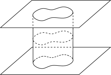
Figure 2: A dyonic instanton. The D2-brane supertube is suspended between two parallel D4-branes.

At this stage, the Higgs zero locus of the dyonic instantons may naturally be identified with the cross-section of the supertubes [4]. To provide further evidence for such identification, it is natural to ask whether the supertubes continue to exhibit its intrinsic properties with additional inputs from its proposed field counterparts, the dyonic instantons. For example, it is well known that the angular momentum of the supertube is given by the curve defining its cross-section [9]. In section 2 of this paper, we would like to show that, by substituting the Higgs zero locus for the cross-section in the expression for supertube angular momentum, such angular momentum is maximized at circular Higgs zero locus, provided the electric charge $Q_{e}$ of the dyonic instanton is kept fixed. This specific property for supertube was first demonstrated in the supergravity contexts [9], here we consider a purely field theoretical calculations and formulate the analogous variational problem. This in turns would require us to set up a dictionary between the conserved charges of dyonic instantons and supertubes. We shall argue that this dictionary is crucial in giving consistent interpretation between our field theory results and the known stringy properties of the supertubes. In addition, we study a T-dual picture of this story in section 2.5, demonstrating that the momentum for the so called “D-helix” [13] (or its S-dual – “supercurve” [14]) has identical functional dependence on its shape as their field theory counterparts known as “wavy instanton strings” [15]. This identification in fact is where such a dictionary is at its clearest.

The identification of the Higgs zero locus with the supertube cross-section leads us to an interesting correspondence: real algebraic curves $\leftrightarrow$ Yang-Mills instantons. The Higgs zero of the dyonic instantons serves as a bridge between these two concepts. Note that the Higgs field does not spoil the original instanton configuration, because the second equation in (1.1) does not cause a back-reaction to the first (self-dual) equation. In this sense the Higgs field is a true probe, with a help of the electric field. The Higgs zero loci are given by algebraic real curves which are defined as polynomial equations of spatial coordinates. In section 3, we examine this intriguing correspondence. We shall see that the degree of the algebraic curves is related to the instanton number, and the splitting property of the curves is manifested physically by well-separated instantons.

2 Maximization of angular momentum

2.1 Dyonic instantons and angular momentum

The dyonic instantons are BPS solutions of ${\cal N}=2$ super Yang-Mills(-Higgs) theory in 1+4 dimensions [3]. In view of the correspondence to the D-branes, we concentrate on SU(2) gauge group provided by the two parallel D4-branes for simplicity. The Higgs zero loci can form non-trivial loops when we have more than one instanton, and they appear as the monopole strings in the 1+4 dimensions. A complete treatment of arbitrary instanton numbers would require solving the intricate full ADHM constraints. However in this section we shall focus on the case of two instantons where one can bypass such difficulties, and we shall extensively utilize the results obtained by S. Kim and K. Lee [4]. They explicitly solved the equations (1.1) using the ADHM method inspired by the Jackiw-Nohl-Rebbi (JNR) ansatz [16],

$$A_{\mu}(x)=\frac{i}{2}\sigma^{a}\bar{\eta}_{\mu\nu}^{a}\partial_{\nu}\log H_{\rm JNR}(x),\quad H_{\rm JNR}(x)\equiv\sum_{i=0}^{2}\frac{s_{i}}{|y_{i}|^{2}}\ ,$$ (2.3)

where $\bar{\eta}^{a}_{\mu\nu}$ is the anti-self-dual ’t Hooft tensor and $y_{i\mu}\equiv x_{\mu}-a_{i\mu}$. The parameters specifying the instantons are the three scalar moduli $s_{0},s_{1},s_{2}$ which are real and positive, while the three position moduli are labeled as $a_{0\mu},a_{1\mu},a_{2\mu}$, where $\mu=1,\dots,4$ labeling the four spatial directions. Note that for two instantons, this ansatz has enough number of the degrees of freedom to sweep the entire instanton moduli space. Without losing generality, we can rotate the configuration and set $a_{i1}=a_{i2}=0$ ($i=0,1,2$). Other moduli of the dyonic instanton are the spatially asymptotic values $q^{a}\sigma^{a}$ of the Higgs field $\phi$. For simplicity we consider the probe Higgs field with $q^{1}=q^{2}=0$ which gives the Higgs zero on the 3-4 plane and was considered in [4] in details:

$$\phi(x)\big{|}_{y_{i1}=y_{i2}=0}=\frac{q^{3}\sigma_{3}}{(s_{0}+s_{1}+s_{2})H_{\rm JNR}(x)}\frac{X(x)}{|y_{0}|^{2}|y_{1}|^{2}|y_{2}|^{2}}\ .$$ (2.4)

Here we have defined a polynomial function

$$X(x)\equiv\sum_{i=0}^{2}\left(\!s_{i}^{2}|y_{i+1}|^{2}+2s_{i}s_{i+1}y_{i}\!\cdot\!y_{i+1}-\frac{4\left(y_{i}\!\times\!y_{i+1}\right)\sum_{j=0}^{2}(a_{j}\!\times\!a_{j+1})}{\sum_{j=0}^{2}(s_{j}s_{j+1})^{-1}|a_{j}\!-\!a_{j+1}|^{2}}\right)|y_{i+2}|^{2}\ ,\;\;$$ (2.5)

where $\vec{y}_{i}\equiv\vec{x}-\vec{a}_{i}$ are two dimensional vectors on the 3-4 plane, and the cross product is defined as $y_{i}\times y_{j}\equiv y_{i3}y_{j4}-y_{i4}y_{j3}$.

Explicit solution (2.4) shows [4] that the Higgs zero locus is given by the following real algebraic curve

$$X(x)=0.$$ (2.6)

The electric charge of the dyonic instanton is given as

$$Q_{\rm e} = {\rm tr}\int\!d^{4}x\;\partial_{\mu}(E_{\mu}\phi)$$ (2.7)

$$= \frac{8\pi^{2}(q^{3})^{2}}{(s_{0}\!+\!s_{1}\!+\!s_{2})^{2}}\left\{\sum_{i=0}^{2}s_{i}s_{i+1}|a_{i}-a_{i+1}|^{2}-\frac{4\sum_{i=0}^{2}(a_{i}\times a_{i+1})^{2}}{\sum_{j=0}^{2}(s_{j}s_{j+1})^{-1}|a_{j}-a_{j+1}|^{2}}\right\}\ .\quad$$

One can obviously see that both $X(x)=0$ and $Q_{\rm e}$ are invariant under the overall scaling of the scalar moduli $s_{i}$, which are defined projectively.

The identification between the supertube in string theory and dyonic instantons in field theory naturally leads one to further identify the Higgs zero locus $X=0$ with the curve defining supertube cross-section. The ideal place to test such further identification is to consider the angular momentum. According to [9], the angular momentum of the supertube is given by

$$L=\oint_{-\pi}^{\pi}\!d\theta\left(x_{3}\frac{\partial x_{4}}{\partial\theta}-x_{4}\frac{\partial x_{3}}{\partial\theta}\right)\,,$$ (2.8)

where $\theta$ is the coordinate on the curve defining the cross-section. Suppose we made such further identification between the curves in field theory and string theory. Once the ADHM data $(s_{i},a_{i\mu})$ is provided for the dyonic instanton, one can then compute $X=0$ and obtain the curve, and substitute this curve profile into (2.8) to compute the angular momentum for the supertube. The idea here is that we pose a variational problem in field theory which extremizes (2.8), with the dyonic instanton charges fixed. This is related to the similar variational problem for the supertube in string theory, with the supertube charges fixed [14]. Even though we are varying essentially the same integral (2.8), however these two problems are not a priori identical, as the charges which we kept fixed in the field theory and string theory can be different functionals of the curves. To show these two problems can be identified, one has to propose some kind of dictionary which relates the charges in these two theories, and we shall explain such dictionary further in the next subsection 2.2. Conversely we shall see in section 2.4 that, for fixed electric charge $Q_{e}$ of the dyonic instanton, the angular momentum (2.8) calculated from the Higgs zero locus is maximized when it forms a circle, this provides strong evidence for such dictionary between the charges.

To make the distinctions clear, one should first note that the definition (2.8) for the supertube only captures the angular momentum along the Higgs zero locus given by (2.6), and this generally differs from the usual field theoretical definition for the angular momentum of dyonic instanton, which is given by a four dimensional integral [4, 17],

$$\widetilde{L}_{\mu\nu}=\int\!d^{4}x\left(x_{\mu}T_{0\nu}-x_{\nu}T_{0\mu}\right)$$ (2.9)

with $T_{\mu\nu}$ being the energy momentum tensor of the 1+4 dimensional Yang-Mills theory.

In the following, we shall first explain the proposed dictionary between charges in more details. We then give the support for such dictionary by demonstrating that for fixed $Q_{e}$, the angular momentum for the supertube as defined by (2.8) is maximized when the Higgs zero locus forms a circle. To do so, we derive in section 2.3 a condition for $X=0$ to give a circle in terms of the ADHM data of the instantons. In section 2.4, we show that perturbations around the ADHM data giving the circle always decrease the angular momentum. There we also present some numerical calculations. In addition, we consider a more evident example of the dictionary between charges given in 2.5, where D-helices/supercurves [13, 14] (embedded in two coincident D5-branes) are identified with wavy instanton string solutions [15] in 1+5 dimensional SU(2) Yang-Mills theory. For this case, the dictionary between the charges is completely proven.

2.2 Dictionary between supertubes and dyonic instantons

Here we would like to discuss further the dictionary mentioned earlier between the conserved charges for the dyonic instantons and the supertubes. On one hand if we had assumed such dictionary, then variational problem in field theory proposed earlier would be identical to the one for the supertubes in string theory. On the other hand, our results in section 2.4, which demonstrates that the angular momentum (2.8) calculated from the Higgs zero locus maximizes at the circle for fixed dyonic instanton charges, can be regarded as the supporting evidence for such dictionary.

First let us list the standard relations between the various parameters in string theory and the 1+4 dimensional SU(2) Yang-Mills-Higgs theory. The distance between the D4-branes, $l$, is related to the Higgs expectation value at asymptotic infinity,

$$l=2\pi l_{s}^{2}\cdot 2q^{3}$$ (2.10)

with $l_{s}$ being the string length. The gauge coupling constant $e$ in the Yang-Mills-Higgs theory is related to the string coupling constant through the tension of the D4-brane as $1/e^{2}=(1/2)T_{\rm D4}(2\pi l_{s}^{2})^{2}$ which can be simplified as

$$e^{2}=8\pi^{2}l_{s}g_{s}\,.$$ (2.11)

Consider the BPS equations (1.1), it describes a dyonic instanton whose energy is given in terms of its charges [3]:

$${\cal E}_{\rm dyonic}=\frac{8\pi^{2}}{e^{2}}\kappa+\frac{2}{e^{2}}Q_{\rm e}\ .$$ (2.12)

Here $\kappa$ is the instanton number, and $Q_{\rm e}$ is the electric charge of the dyonic instanton given in equation (2.7). This energy should be equal to that of the supertube. The supertube is described as a configuration of D2-brane worldvolume theory, and the energy is just given by the tension of the supertube (per unit length) times its length $l$ (which equals the distance between the two D4-branes),

$${\cal E}_{\rm supertube}=l\int_{-\pi}^{\pi}\!\!d\theta\;{\cal H}.$$ (2.13)

Here $\theta$ is the cylindrical coordinate parameterizing the cross-section of the supertube surface, and ${\cal H}$ is the energy density of the supertube given in terms of a low energy D2-brane worldvolume theory. Using the decomposition of the Hamiltonian by the D-brane/F-string charges given in [8], we arrive at the expression

$${\cal E}_{\rm supertube}=l\left(T_{\rm D0}Q_{\rm D0}+2\pi T_{\rm F1}Q_{\rm F1}\right)\ .$$ (2.14)

Here $T_{\rm F1}$ $(Q_{\rm F1})$ and $T_{\rm D0}$ $(Q_{\rm D0})$ are the tension (charge) of the F-strings and the D0-branes respectively. Comparing (2.12) and (2.14), and using the standard relations (2.10) and (2.11), we propose the dictionary

$$\frac{\kappa}{q^{3}}=4\pi l_{\rm s}^{2}Q_{\rm D0}\ ,$$ (2.15)

$$\frac{Q_{\rm e}}{q^{3}}=16\pi^{3}l_{\rm s}g_{\rm s}Q_{\rm F1}\ .$$ (2.16)

Suppose the identifications (2.15) and (2.16) are valid, they would imply that fixing $\kappa$ and $Q_{e}$ for dyonic instantons corresponds precisely to keeping fixed the D0 and F1 charges for the supertube, hence the two variational problems can be identified and the maximal angular momentum occurs at the circular shape. Conversely, we will show in section 2.4 that angular momentum for the supertube (2.8) calculated from the Higgs zero locus is maximized when it becomes circular, for given $\kappa$ and $Q_{e}$, this should then be interpreted as a supporting evidence for the dictionary (2.15) and (2.16).

The identification (2.15) and (2.16) means not only that the values of the charges are identical, but also that the charges are identical functionals of the curves which are defined by the Higgs zero locus for the dyonic instantons and by the cross-section for the supertubes. This is the main point of the present paper, so here we explain in details the logic of our reasoning given briefly above.

The supertubes are described by the following fields on the D2-brane: the magnetic field $B(\theta)$, the conjugate momentum $\Pi_{z}(\theta)$ with respect to the gauge field, and the transverse scalar field $y_{\mu}(\theta)$. The supertubes satisfy the relation

$$B\Pi_{z}=T_{\rm D2}|y_{\mu}^{\prime}(\theta)|^{2}.$$ (2.17)

The charges are defined as $Q_{\rm D0}=(1/2\pi)\int\!d\theta\;B$, $Q_{\rm F1}=(1/2\pi)\int\!d\theta\;\Pi_{z}$. Using reparameterization of $\theta$, we may put the magnetic field constant. Through the equation (2.17), the electric charge is dependent on the shape of the cross-section $y_{\mu}(\theta)$. Given the cross-section $y_{\mu}$, we can define the angular momentum of the supertube $L_{\rm supertube}$ as in (2.8), thus the angular momentum is a functional of the cross-section, $L_{\rm supertube}[y_{\mu}]$. On the other hand, for the dyonic instantons, the instanton number $\kappa$ is fixed while the electric charge $Q_{\rm e}$ is a function of the ADHM data $(s_{i},a_{i})$. The Higgs zero locus is defined by the ADHM data, so the curve $x_{\mu}=\hat{x}_{\mu}(\theta)$ is given as a solution of $X(s_{i},a_{i},x)=0$. The angular momentum $L$ is defined by this $\hat{x}_{\mu}$, as explained in section 2.1, so $L$ is a functional of $\hat{x}_{\mu}$, $L=L[\hat{x}_{\mu}]$. Since the definition is the same as the supertube, we should note that the $\hat{x}_{\mu}$ dependence in $L$ is the same as the $y_{\mu}$ dependence in $L_{\rm supertube}$.

From these precise definitions, the meaning of the “dictionary” (2.15) and (2.16) is clear. The left hand side of (2.16) is a function of $(s_{i},a_{i})$ while the right hand side is a functional of $y_{\mu}$. Note that we can extract the information of the ADHM data $(s_{i},a_{i})$ from the curve $\hat{x}_{\mu}$, so implicitly $Q_{\rm e}$ is a functional of the curve $\hat{x}_{\mu}$. The proposed dictionary means that, the functional dependence of the both sides are the same, if we identify the curve $\hat{x}_{\mu}$ with the cross-section $y_{\mu}$. The result of section 2.4 will strongly support that this is correct, since the variational problems in the two pictures exhibit the same property: the angular momentum is maximized when the curve is circular. This in turn means that the identification of the Higgs zero locus with the supertube cross-section, $\hat{x}_{\mu}=y_{\mu}$, is correct.

2.3 Conditions for circular cross section

In this and next subsections, we shall show that the maximization of the supertube angular momentum (2.8) computed from the Higgs zero locus $X=0$ is achieved when the locus is circular. First, let us study for which value of the ADHM data the curve $X=0$ becomes circular.

For the circular cross-section to appear, i.e. $(x_{3}^{2}+x_{4}^{2})=r_{0}^{2}$, it is necessary for $X$ to take the following form

$$A(x_{3}^{2}+x_{4}^{2})^{2}+B(x_{3}^{2}+x_{4}^{2})+C=0\,,$$ (2.18)

that is a quadratic equation in $(x_{3}^{2}+x_{4}^{2})$, the radius of the circle $r_{0}$ is then given by the root of this equation. Here we show that the Higgs zero locus (2.6) forms a circular shape (2.18) with a unique set of the nine parameters $(s_{i},a_{i\mu})$ ($i=0,1,2$ and $\mu=3,4$), up to the overall scaling of $s_{i}$ and the rotation around the origin $x_{3}=x_{4}=0$.

Consider the most general fourth order polynomial for $x_{3}$ and $x_{4}$,

$$b_{4}x_{3}^{4}+b_{3}x_{3}^{3}+b_{2}x_{3}^{2}+b_{1}x_{3}+c_{4}x_{4}^{4}+c_{3}x_{4}^{3}+c_{2}x_{4}^{2}+c_{1}x_{4}+k$$

$$+d_{1}x_{3}x_{4}+d_{2}x_{3}^{2}x_{4}^{2}+f_{1}x_{3}x_{4}^{2}+f_{2}x_{3}^{2}x_{4}+h_{1}x_{3}x_{4}^{3}+h_{2}x_{3}^{3}x_{4}\,.$$ (2.19)

Clearly by comparing (2.5) with (2.18) and (2.19), we seem to have more conditions than the number of variables. However, $X$ as defined in (2.5) belongs to a special subset of these general polynomials, simple expansion can show that for $X$, the followings are satisfied identically:

$$b_{4}=c_{4}=\frac{1}{2}d_{2}=(s_{0}+s_{1}+s_{2})^{2}\,,\quad b_{3}=f_{1}\,,\quad c_{3}=f_{2}\,,\quad h_{1}=h_{2}=0\,.$$ (2.20)

We are left with precisely six conditions

$$b_{3}=0\,,~{}c_{3}=0\,,~{}d_{1}=0\,,~{}b_{2}=c_{2}\,,~{}b_{1}=0\,,~{}c_{1}=0\,.$$

The first four conditions give rise to the following equations for $a_{i3}$ and $a_{i4}$:

$$a_{03}(s_{1}+s_{2})+a_{13}(s_{0}+s_{2})+a_{23}(s_{0}+s_{1})=0\,,$$ (2.21)

$$a_{04}(s_{1}+s_{2})+a_{14}(s_{0}+s_{2})+a_{24}(s_{0}+s_{1})=0\,,$$ (2.22)

$$s_{0}(a_{13}a_{24}+a_{14}a_{23})+s_{1}(a_{03}a_{24}+a_{04}a_{23})+s_{2}(a_{03}a_{14}+a_{04}a_{13})=0\,,$$ (2.23)

$$s_{0}(a_{13}a_{23}-a_{14}a_{24})+s_{1}(a_{03}a_{23}-a_{04}a_{24})+s_{2}(a_{03}a_{13}-a_{04}a_{14})=0\,.$$ (2.24)

The first two equations are solved straightforwardly as

$$a_{03}=\frac{-\left(a_{23}(s_{0}\!+\!s_{1})+a_{13}(s_{0}\!+\!s_{2})\right)}{(s_{1}+s_{2})}\,,\quad a_{04}=\frac{-\left(a_{24}(s_{0}\!+\!s_{1})+a_{14}(s_{0}\!+\!s_{2})\right)}{(s_{1}+s_{2})}\,.$$ (2.25)

Then (2.23) is solved as

$$a_{13}=\frac{-a_{23}s_{1}(a_{24}(s_{0}+s_{1})+a_{14}s_{2})}{s_{2}(a_{24}s_{1}+a_{14}(s_{0}+s_{2}))},$$ (2.26)

where we have implicitly assumed that the denominator is non-vanishing. Using these we solve (2.24) as

$$a_{23}=\pm\sqrt{\frac{s_{2}}{s_{0}s_{1}(s_{0}+s_{1}+s_{2})}}(a_{24}s_{1}+a_{14}(s_{0}+s_{2})).$$ (2.27)

We choose the negative sign in the right hand side of (2.27) for simplicity. The condition $b_{1}=0$ is then simplified to

$$(s_{0}+s_{2})(s_{0}+s_{1}-2s_{2})a_{14}=(s_{0}+s_{1})(s_{0}+s_{2}-2s_{1})a_{24}.$$ (2.28)

It is straightforward to show that this condition is compatible with the last equation $c_{1}=0$ with (2.25)-(2.27) only if $s_{0}=s_{1}=s_{2}$. All the constraints are solved with this as

$$a_{03}=-a_{13}-a_{23}\,,\;a_{04}=-a_{24}-a_{14}\,,\;a_{13}=-a_{23}\frac{a_{14}\!+\!2a_{24}}{a_{24}\!+\!2a_{14}}\,,\;a_{23}=\frac{-(a_{24}\!+\!2a_{14})}{\sqrt{3}}\,.$$

Substituting these into $X$, we find

$$\frac{X}{(s_{0})^{2}}=9(x_{3}^{2}\!+\!x_{4}^{2})^{2}+4(a_{14}^{2}\!+\!a_{14}a_{24}\!+\!a_{24}^{2})(x_{3}^{2}\!+\!x_{4}^{2})-\frac{16}{3}(a_{14}^{2}\!+\!a_{14}a_{24}\!+\!a_{24}^{2})^{2}\hskip 28.45274pt$$ (2.29)

which certainly gives a single circle. The example of the ADHM data given in [4],

$$s_{0}^{(0)}=s_{1}^{(0)}=s_{2}^{(0)}=1\,,\;(a_{03}^{(0)},a_{04}^{(0)})=(-R,0)\,,\;$$ (2.30)

$$(a_{13}^{(0)},a_{14}^{(0)})=(R/2,-\sqrt{3}R/2)\,,\;(a_{23}^{(0)},a_{24}^{(0)})=(R/2,\sqrt{3}R/2),$$

is a particular representative of our general solution. The example is the unique data giving the circle, up to rotation around the origin and parallel transport on the 3-4 plane.

2.4 Maximization around circular profile

Let us study the perturbations from the circular Higgs zero found above and see how the angular momentum (2.8) is maximized there. It is enough to consider the representative (2.30) according to the uniqueness shown in the previous subsection. The radius of the circle is given by

$$r_{0}=\sqrt{\frac{\sqrt{13}-1}{6}}R,$$ (2.31)

thus the angular momentum for the configuration (2.30) is given by

$$L=2\pi r_{0}^{2}=2\pi\frac{\sqrt{13}-1}{6}R^{2}=\frac{\sqrt{13}-1}{48\pi}\frac{Q_{\rm e}}{(q^{3})^{2}}.$$ (2.32)

In the last equation we have used the electric charge for this ADHM data, $Q_{\rm e}=16\pi^{2}(q^{3})^{2}R^{2}$.

2.4.1 Showing the extremum

The small perturbations from the point (2.30) are given by

$$s_{i}\equiv 1+\delta s_{i}\,,\quad a_{i3}\equiv a_{i3}^{(0)}+R\delta a_{i3}\,,\quad a_{i4}\equiv a_{i4}^{(0)}+R\delta a_{i4}\,.$$ (2.33)

Let us consider the first order in perturbation. We expand the function $X$ around the data (2.30). A straightforward calculation gives

$$X=\hat{X}+X_{i}\delta s_{i}+RX_{i3}\delta a_{i3}+RX_{i4}\delta a_{i4}+{\cal O}(\delta^{2}),$$ (2.34)

where $\hat{X}$ is the polynomial given in equation (2.29) and $X_{i},X_{i3}$ and $X_{i4}$ are homogeneous polynomials of $(x_{3},x_{4},R)$, whose explicit expressions can be obtained easily (we don’t show them here).

In solving $X=0$, we may use the following parameterization for the coordinates $x_{3}$ and $x_{4}$:

$$x_{3}\equiv(r_{0}+R\delta r(\theta))\cos(\theta)\,,\quad x_{4}\equiv(r_{0}+R\delta r(\theta))\sin(\theta)\,.$$ (2.35)

The fluctuation of ${\cal O}(\delta r)$ coming from the substitution of this into $\hat{X}$ is then given by

$$\hat{X}=0+\sqrt{78(-1+\sqrt{13})}R^{4}\delta r+{\cal O}((\delta r)^{2})\,.$$ (2.36)

Therefore we may solve the equation $X=0$ to derive the expression of the deformation of the radius $\delta r$ written in terms of the moduli deformation $\delta s$ and $\delta a$ as

$$\delta r(\theta)=\frac{-\left[X_{i}\delta s_{i}+RX_{i3}\delta a_{i3}+RX_{i4}\delta a_{i4}\right]_{x_{3}=r_{0}\cos\theta,\;x_{4}=r_{0}\sin\theta}}{\sqrt{78(-1+\sqrt{13})}R^{4}}\,.$$ (2.37)

With this, we can compute the angular momentum along the Higgs zero locus as

$$L = \int\!d\theta(r_{0}^{2}+2r_{0}R\delta r+{\cal O}((\delta r)^{2}))$$ (2.38)

$$\simeq 2\pi r_{0}^{2}-\frac{\pi}{3}(\sqrt{13}-1)R^{2}\left[\frac{-2}{3}\delta a_{03}+\frac{1}{3}\delta a_{13}+\frac{1}{\sqrt{3}}\delta a_{14}+\frac{1}{3}\delta a_{23}+\frac{1}{\sqrt{3}}\delta a_{24}\right]\,.\hskip 28.45274pt$$

We need to evaluate how the electric charge $Q_{\rm e}$ responds to the perturbation. In other words, keeping $Q_{\rm e}$ fixed imposes a linear constraint among the deformation parameters. A straightforward calculation then gives

$$\frac{Q_{\rm e}}{(q^{3})^{2}16\pi^{2}R^{2}}=1+\frac{-2}{3}\delta a_{03}+\frac{1}{3}\delta a_{13}+\frac{1}{\sqrt{3}}\delta a_{14}+\frac{1}{3}\delta a_{23}+\frac{1}{\sqrt{3}}\delta a_{24}+{\cal O}(\delta^{2})\,,$$

thus fixing the electric charge is equivalent to the constraint

$$\delta a_{03}=\frac{1}{2}\left[\delta a_{13}+\sqrt{3}\delta a_{14}+\delta a_{23}+\sqrt{3}\delta a_{24}\right]\,.$$ (2.39)

Now it is obvious that the perturbation of $Q_{\rm e}$ coincides with the perturbation of $L$ (2.38). This means that, if we fix the electric charge $Q_{\rm e}$, then the angular momentum does not change at the first order perturbation. We showed that, for the angular momentum, (2.30) is a stationary point in the moduli space. This is a strong evidence that the angular momentum is maximized at the circular configuration (2.30). We shall demonstrate next that this is indeed a local maximum, by considering the perturbation at second order.

2.4.2 Showing the maximum

We have nine moduli parameters $(s_{i},a_{i3},a_{i4})$ in general, these are too many variables to analyze exactly at the second order in their perturbations. Thus, for simplicity, we restrict ourselves to treat a subspace of the moduli space, and consider a more manageable situation with only four parameters $\delta a_{03},\ \delta a_{13},\ \delta a_{23}$ and $\delta a_{04}$ while fixing all the others to the values (2.30), to demonstrate the maximization of the angular momentum.

The variation of the electric charge $Q_{\rm e}$ with respect to this perturbation is then

$$\frac{Q_{\rm e}}{16\pi^{2}(q^{3})^{2}R^{2}} = 1+\frac{1}{3}\left(-2\delta a_{03}\!+\!\delta a_{13}\!+\!\delta a_{23}\right)+\frac{4}{9}\left((\delta a_{03})^{2}\!+(\delta a_{13})^{2}\!+(\delta a_{23})^{2}\!+(\delta a_{04})^{2}\right)$$

$$-\frac{2}{9}\left(\delta a_{03}\delta a_{13}+\delta a_{13}\delta a_{23}+\delta a_{23}\delta a_{03}-\sqrt{3}\delta a_{13}\delta a_{04}+\sqrt{3}\delta a_{23}\delta a_{04}\right)+{\cal O}(\delta^{3})\,.$$

We want to fix the value of the electric charge $Q_{\rm e}=16\pi^{2}R^{2}(q^{3})^{2}$ which is given by (2.30). This leads to a constraint which can be solved for $\delta a_{23}$ up to this order, as

$$\delta a_{23} = \left[2\delta a_{03}-\delta a_{13}\right]+\left[-4(\delta a_{03})^{2}-4(\delta a_{13})^{2}-\frac{4}{3}(\delta a_{04})^{2}\right.$$ (2.40)

$$\hskip 56.9055pt\left.+\ 8\delta a_{03}\delta a_{13}+\frac{4}{\sqrt{3}}\delta a_{03}\delta a_{04}-\frac{4}{\sqrt{3}}\delta a_{13}\delta a_{04}\right]+{\cal O}(\delta^{3})\,.$$

Let us next solve the condition $X=0$ by using the parameterization (2.35). Plugging the perturbed variables into the equation $X=0$, we can express $\delta r(\theta)$ in terms of $\delta a_{03},\ \delta a_{13},\ \delta a_{04}$ and $\delta a_{23}$, up to their second orders. The explicit expressions are not so illuminating, however the resultant angular momentum up to the second order takes a very simple form

$$L=2\pi r_{0}^{2}-2\pi R^{2}\alpha\left(-\sqrt{3}\delta a_{03}+\sqrt{3}\delta a_{13}+\delta a_{04}\right)^{2}\!\!,\;\alpha\equiv\frac{137\sqrt{13}\!-\!13^{2}}{13^{2}\cdot 3^{2}}(\approx 0.21)\,.\hskip 28.45274pt$$ (2.41)

Here we have eliminated $\delta a_{23}$ by using (2.40). As expected, the first order terms are vanishing and the coefficient of the second order is negative, $-2\pi R^{2}\alpha$. This is the corroboration of our claim that (2.30) gives the unique maximum of the angular momentum.

It is not so easy to increase the number of perturbation parameters, thus we analyze here some other sets of parameters to illustrate the point. For the set $(\delta a_{03},\ \delta a_{23},\ \delta a_{04},\ \delta a_{14})$, the same procedures give the angular momentum

$$L=2\pi r_{0}^{2}-2\pi R^{2}\alpha\left[\left(-\sqrt{3}\delta a_{03}+\delta a_{04}-2\delta a_{14}\right)^{2}+3\left(\delta a_{14}\right)^{2}\right].$$ (2.42)

For the set $(\delta a_{03},\ \delta a_{23},\ \delta a_{14},\ \delta a_{24})$, we obtain

$$L=2\pi r_{0}^{2}-2\pi R^{2}\alpha\left[\left(-\sqrt{3}\delta a_{03}-2\delta a_{14}+\delta a_{24}\right)^{2}+3\left(\delta a_{14}-\delta a_{24}\right)^{2}\right].$$ (2.43)

For the set $(\delta a_{23},\ \delta a_{04},\ \delta a_{14},\ \delta a_{24})$, the angular momentum is of the form

$$L=2\pi r_{0}^{2}-2\pi R^{2}\alpha\left[\left(\delta a_{04}-2\delta a_{14}+\delta a_{24}\right)^{2}+3\left(\delta a_{14}-\delta a_{24}\right)^{2}\right].$$ (2.44)

In all cases, the angular momentum (2.8) is maximized at the circular Higgs zero locus (2.30).

2.4.3 Numerical evaluation

Since the analytical evaluation is intricate, we turn to a numerical evaluation of the angular momentum (2.8) for given ADHM data of the instantons. We find that, even if we include perturbation of the parameters $s_{i}$ in addition to $a_{i\mu}$, the angular momentum is still maximized at the circular profile (2.30).

Figure 3: $s_{0}=1$.

Figure 4: $s_{0}=4$.

Figure 5: $s_{0}=13$.

Figure 6: $s_{0}=25$.

To illustrate the numerical simulations, here we present some peculiar examples of the deformation to the circular profile. The most interesting property of the loops given by the Higgs zero loci is that they split as one changes the ADHM data. See Fig. 6, $\cdots$, Fig. 6. We have chosen $a_{03}=-\sqrt{s_{0}}R$ and varied $s_{0}$, while other variables are kept to be (2.30). As before, we keep the electric charge fixed, which determines the parameter $R$. For $s_{0}=1$ which is (2.30), we have a circle, but as we increase the parameter $s_{0}$, the circle is deformed and splits into two loops, and the loops continuously shrink to vanishing size at large $s_{0}$. The large $s_{0}$ limit is identical to the ’t Hooft instanton, as seen in (2.3) and discussed in [4].

The angular momenta (2.8) calculated from the Higgs zero loci are summarized in the following table. One can immediately see that it is maximized at $s_{0}=1$ of (2.30). The cases with $s_{0}<1$ show the maximization at $s_{0}=1$, too, though we have not listed the evaluated numerical values. The angular momenta in the table are measured in the unit of $Q_{\rm e}/(16\pi^{2}(q^{3})^{2})$.

	$s_{0}$	angular momentum
Fig. 6	1	2.73 $(=2\pi(\sqrt{13}-1)/6)$
Fig. 6	4	2.47
Fig. 6	13	1.38
Fig. 6	25	0.57

2.5 Wavy instanton strings and supercurves/D-helices

To illustrate the dictionary given in section 2.2, here we study the IIB counterpart of the supertube and the corresponding BPS soliton in Yang-Mills theory. We shall see that, interestingly, in this case the dictionary can be proven as a functional of the curves.

When we take a T-duality along the axial direction of the supertube, we find a super D-helix which is a helical D1-brane moving with the speed of light along its axis [13]. As an example, let us consider a perfectly circular D-helix with radius $R$ for definiteness (the radius is defined as a trajectory projected on a plane perpendicular to the axis), which is the T-dual of a perfectly circular supertube with the same radius. The Hamiltonian of the super D-helix is given by ${\cal H}=T_{\rm D1}|B|+|\Pi|$, where $\Pi$ is the momentum of the D-helix along the axis, and $B$ is the slope of the D-string along the axis, namely the pitch of the D-helix is given by $2\pi RB$. The relation to the supertube is apparent: in view of (2.14), the momentum corresponds to the F1 charge of the supertube, and the slope corresponds to the D0-brane charge. The super D-helix satisfies $\sqrt{2\pi l_{\rm s}^{4}g_{\rm s}|\Pi B|}=R$, which means that the speed of the D-helix along the axis is equal to the speed of light. By the T-duality, this is equivalent to the equation $E=\pm 1/2\pi l_{\rm s}^{2}$ of the supertube. Moreover, the super D-helix preserves a quarter of the bulk supersymmetries, which is the same as the supertube.

Supercurves formulated in [14] are the objects that are S-dual to the D-helices, and there it was found that the supercurves, which are fundamental strings traveling with the speed of light, allow arbitrary deformation of the shape as long as the speed is maintained, which is analogous to the supertubes. The Hamiltonian is similar to the above,

$${\cal H}=T_{\rm F1}|Z^{\prime}(\theta)|+|P_{Z}(\theta)|\,.$$ (2.45)

Here $Z(\theta)$ is a scalar field on the worldsheet and specifies the location along the axis of the supercurve, and we can choose the gauge $Z^{\prime}=1$ by using reparameterization of the worldsheet coordinate $\theta$. $P_{Z}$ is the momentum of the supercurve along the axis $Z$. The shape of the supercurve projected onto the plane transverse to the $Z$ direction is given by the other scalar fields $y^{\mu}(\theta)$. The BPS equations of motion shows

$$P_{Z}(\theta)=T_{\rm F1}|y_{\mu}^{\prime}(\theta)|^{2}\,.$$ (2.46)

As long as this relation is satisfied, $y_{\mu}$ dependence in the Hamiltonian vanishes. This is the reason why the supercurves allow almost arbitrary deformations.

It was further shown in [14] that, for fixed total momentum $\int\!d\theta P_{Z}$ of the periodic supercurves, the angular momentum defined by $y_{\mu}(\theta)$ as in (2.8) is maximized when the projected shape $y_{\mu}$ of the supercurve is circular. This is consistent with the T-duality. Since we can apply the same method for the D-helices, in the following we shall use the notation of the supercurves.

In order to find a field theoretical counterpart of the super D-helix, let us consider a T-duality of the situation at hand: a supertube suspended between two parallel D4-branes as we considered for the dyonic instantons in this paper. Taking the T-duality along the transverse direction of the D4-branes, we obtain the super D-helix embedded in coincident two D5-branes. As the supertubes suspended between the D4-branes can be thought of as the 1/4 BPS dyonic instantons in 1+4 dimensions from the D4-brane view point, the super D-helix should be thought of as a 1/4 BPS soliton in a 1+5 dimensional Yang-Mills theory, from the D5-brane view point. Such a 1/4 BPS soliton in 1+5 dimensions was found in [15] as a solution of the 1/4 BPS equations

$$F_{\mu\nu}=*F_{\mu\nu},\quad E_{\mu}=F_{5\mu},\quad E_{5}=0,$$ (2.47)

with the Gauss’s law $D_{\mu}E_{\mu}+D_{5}E_{5}=0$ ($\mu,\nu=1,2,3,4$). The solution is called wavy instanton strings, which extends along the $x^{5}$ axis on which an electric wave runs with the speed of light. The $x^{5}$ direction is identified with the $Z$ direction of the D-helices/supercurves.

Notice that all the BPS equations for the wavy instanton string (including the Gauss’s law) and their solutions lead to those for the dyonic instantons by the dimensional reduction $\partial_{5}=0$ and $A_{5}=-\phi$ [15]. The dimensional reduction can be naively thought of as embodiment of the T-duality in field theories, analogous to the well-known dimensional reduction from instantons (D4-D0 system) to monopoles (D3-D1 system).

The BPS equations (2.47) can be solved by choosing $\partial_{0}=\partial_{5}$ and $A_{0}=A_{5}$ in any instanton background [15]. Namely, concrete solutions of the wavy instanton string can be found by promoting the moduli parameters $y^{\mu}$ for the center of the instantons to be arbitrary functions of the combination $x^{0}+x^{5}$ as [15]

$$A_{\mu}=A_{\mu}^{\rm inst}\left(x^{\mu}-y^{\mu}(x^{0}+x^{5})\right)\,,\quad A_{0}=A_{5}=-\frac{\partial y^{\mu}}{\partial x^{0}}A_{\mu}\,.$$ (2.48)

For example, a helical wavy instanton string with circular profile on the projected plane can be obtained by choosing the particular functions

$$y^{3}=R\cos\left(\frac{x^{0}+x^{5}}{RB}\right),\quad y^{4}=R\sin\left(\frac{x^{0}+x^{5}}{RB}\right),$$ (2.49)

while $y^{1},y^{2}$ are constants. This helical wavy instanton string has the radius $R$, its velocity is the speed of right and its pitch is $2\pi RB$, the same as the “circular” super D-helix described above.

Obviously, the correspondence between the super D-helix and helical wavy instanton string is more transparent than that between the supertubes and the dyonic instantons. Here, we shall directly show that the momentum computed in the field theory language has identical functional dependence on $y^{\mu}$ as that of the supercurve $P_{Z}$. This is a proof of the dictionary analogous to the one proposed in the case of the dyonic instantons $\leftrightarrow$ the supertubes.

The Hamiltonian of the wavy instanton strings is given by

$${\cal H}=\int\!dx^{5}\left[\frac{8\pi^{2}}{e^{2}}\kappa+\frac{2}{e^{2}}\int\!d^{4}x\;{\rm tr}F_{0\mu}F_{5\mu}\right]\,.$$ (2.50)

One can see the complete analogy with the dyonic instanton, (2.12). The second term is the momentum along the $x^{5}$ axis. In comparison to the supercurves/D-helices, the Hamiltonian (2.45) shows that the dictionary is

$$\frac{8\pi^{2}}{e^{2}}\kappa=T_{\rm D1}|Z^{\prime}|\,,\quad\frac{2}{e^{2}}\int\!d^{4}x\;{\rm tr}F_{0\mu}F_{5\mu}=|P_{Z}|\,.$$ (2.51)

The first equation should be understood in the gauge $Z^{\prime}=1$ and with $\kappa=1$, since we consider a single D-helix/supercurve.

The Yang-Mills field strength for the single instanton is given by

$$F^{\rm inst}_{\mu\nu}=\frac{\rho^{2}}{(|x_{\mu}|^{2}+\rho^{2})^{2}}\bar{\eta}_{\mu\nu}^{a}\sigma_{a}.$$ (2.52)

According to the solution (2.48), the location of the center of the wavy instanton string is just given by $x^{\mu}=y^{\mu}(x^{0}+x^{5})$. This is almost clear from the definition, but one can define this location in a gauge invariant manner as a solution to the equations ${\rm tr}\partial_{\mu}(F_{\rho\sigma}F_{\rho\sigma})=0$, for example. With this single instanton solution, let us evaluate the momentum given by the second term of (2.50). From (2.48), it is straightforward to obtain

$$F_{0\mu}=F_{5\mu}=-\frac{\partial y^{\rho}}{\partial x^{5}}F_{\rho\mu}\,.$$ (2.53)

Therefore,

$$\int\!d^{4}x\;{\rm tr}F_{0\mu}F_{5\mu}=\frac{\partial y^{\rho}}{\partial x^{5}}\frac{\partial y^{\sigma}}{\partial x^{5}}\int\!d^{4}x\;{\rm tr}F^{\rm inst}_{\rho\mu}F^{\rm inst}_{\sigma\mu}.$$ (2.54)

Here we have made a shift $x^{\mu}-y^{\mu}(x^{0}+x^{5})\to x^{\mu}$ in the integral since it does not affect the result. The integral can be evaluated with the BPST instanton (2.52), but we just need the dependence on the indices,

$$\int\!d^{4}x\;{\rm tr}F^{\rm inst}_{\rho\mu}F^{\rm inst}_{\sigma\mu}=({\rm const.})\times\bar{\eta}_{\rho\mu}^{a}\bar{\eta}_{\sigma\mu}^{a}=({\rm const.})\times\delta_{\rho\sigma}\,.$$ (2.55)

Thus we find

$$\int\!d^{4}x\;{\rm tr}F_{0\mu}F_{5\mu}=({\rm const.})\times\biggl{|}\frac{\partial y^{\rho}}{\partial x^{5}}\biggr{|}^{2}\,.$$ (2.56)

This is precisely what we have expected in (2.46), in the gauge $dx_{5}/d\theta=Z^{\prime}=1$. The dictionary (2.51) is proven as a functional of the shape of the wavy instanton strings and the supercurves/D-helices.

The virtue of this T-dual example, compared to the dyonic instantons, is that from the first place, the wavy instanton string solution (2.48) includes the functional dependence explicitly. However, the dimension reduction to dyonic instantons is not easy, and so far there are only a limited number of solutions (such as periodic instantons) found to be consistent with the explicit T-duality in string theory picture. It would be interesting if the T-duality in field theories can be formulated more usefully, to provide a route for proving the dictionary of the dyonic instantons, from that of the wavy instanton strings.

3 Algebraic curves capturing ADHM data

3.1 A conjecture

The central concept underlying the analysis in the previous section is that the ADHM data, once it is given, produces a real algebraic curve. This is very intriguing in the sense that ADHM data are generally difficult to interpret, especially when the number of instantons is large. Another difficulty is due to the presence of the gauge orbit among the ADHM data. In view of this, the algebraic real curves (loops) given by the Higgs zero may be a good and effective alternative to capture the information of the instantons.

One may hope that the correspondence is one-to-one and thus the curves may capture all the information of the instantons. (For monopoles, certainly this kind of correspondence exists: spectral curves of monopoles [19], which are Riemann surfaces.) We know that for a given instanton configuration, it defines a Higgs zero, thus the map is at least on-to, for appropriately defined set of algebraic curves (recall that coefficients of the polynomial are related, as seen in section 2.3). In general, the requirement of adjoint $\phi=0$ consists of three real equations, while we have four spatial coordinates $x_{\mu}$, thus resulting in a one dimensional curve. The concept is depicted in Fig. 7.

Figure 7: Correspondence between ADHM data and curves by Higgs zero.

Unfortunately, one can find some counter-examples which shows that the correspondence is not one-to-one. Let us first consider the circle. It is expected that the circular Higgs zero locus appears for any instanton number, there appears to be degeneracy to one another. However, this degeneracy can be lifted if one varies the instanton numbers while keeping fixed all the other parameters involved: the electric charge $Q_{\rm e}$ and the asymptotic Higgs vev $q$. We must note here that the rotation in the plane on which the circle lies does not change the circle. But this rotation changes the instanton profile, as seen in the previous section. One cannot lift this rotationary degeneracy.

Another counter-example already appears in the case of the two instantons. Let us consider ’t Hooft ansatz for the instantons. As briefly mentioned before, the Higgs zero corresponding to the ’t Hooft solutions is just two points and not forming a curve [4]. However, we know that the ’t Hooft instantons have size moduli parameters $s_{i}$ in addition to the location of the instantons. This information of the size is not reflected in the profile of the curve. Even when the curve does not shrink to points, it is insensitive to the overall scaling of $s_{i}$.

Even with these counter-examples, it is still interesting to pursue this direction. Certainly the Higgs zero is a gauge-invariant object, and is simple enough because it is given by just algebraic polynomials. Obviously, location of each instanton is indicated by the Higgs zero, which is certainly true for the probe of the adjoint scalar field.

In the following, we first count the degree of the polynomial $X$ which defines the Higgs zero, and show that the degree is bounded by the instanton number $\kappa$. Therefore, when a closed curve is given in terms of a polynomial (as usual for algebraic curves), the degree of it gives the minimal number of instantons necessary for reproducing the curve as a Higgs zero. This is analogous to the spectral curves of monopoles [19], where the degree of the polynomial defining the spectral curve (which is related to the genus of the corresponding Riemann surface) is determined by monopole number. To reproduce any curve which is not expressed by any polynomial, we need infinite number of instantons. The importance of this interesting limit $\kappa\to\infty$ has been pointed out in [20]. Furthermore, we must note that some polynomials may have no corresponding ADHM data. We have seen in the previous section that some coefficients in $X$ are related to each other.

We shall show in section 3.3 that when some of the instantons are located far away from the rest, the curves given by $X=0$ splits into two parts. This splitting property should be endowed with the algebraic curves, because naively the location of the instantons is specified by the curves.

3.2 Degree of algebraic curve and instanton number

3.2.1 JNR instantons

To see how the degree of the polynomial $X$ is related to the data of the instantons appearing in the ADHM construction, we first consider the JNR $\kappa$ instantons. A similar counting for the full ADHM construction will be given later. The ADHM construction of the Higgs solution [3, 4, 21] for the JNR ansatz (2.3) is given by equation (3.8) of [4] as

$$\phi(x)=\frac{1}{s_{\Sigma}H_{\rm JNR}(x)}\left[\bar{Z}(x)qZ(x)+Q(x)\right]$$ (3.57)

with $q=q^{i}\sigma_{i}$ and $s_{\Sigma}=\sum_{i=0}^{\kappa}s_{i}$. In order for $\phi$ to be constant at spatial infinity, the degree of polynomial $\bar{Z}(x)qZ(x)+Q(x)$ should be same as that of ${\rm deg}(H_{\rm JNR})=-2$. Indeed, the definition of $Z$ and $Q$ are given [4] by

$$Z(x)=\sum_{i=0}^{\kappa}\frac{s_{i}y_{i\mu}}{|y_{i}|^{2}}\ e_{\mu},\quad Q(x)=s_{0}^{4}\Lambda^{T}\left\{\frac{1}{Y}-\frac{1}{y_{0}}\right\}KpK\left\{\frac{1}{\bar{Y}}-\frac{1}{\bar{y}_{0}}\right\}\Lambda.$$ (3.58)

Clearly the degrees of $\bar{Z}qZ$ and $Q$ are $-2$. Here we have defined a representation of the quaternion as $e_{\mu}\equiv(i\vec{\sigma},\ 1_{2\times 2})$ and $y_{i}=(x_{\mu}-a_{i\mu})e_{\mu}$. $p$ is a quaternionic $\kappa\times\kappa$ matrix which is determined by equation (3.3) in [4]. $Y$ is a quaternionic diagonal matrix $Y={\rm diag}\left(y_{1},y_{2},\cdots,y_{\kappa}\right)$. $\Lambda$ is a row vector with $\kappa$ real constant components, $\Lambda=\left(s_{1}^{2}/s_{0}^{2},s_{2}^{2}/s_{0}^{2},\cdots,s_{\kappa}^{2}/s_{0}^{2}\right)$, and $K$ is a constant matrix taking value in $GL(\kappa,{\bf C})$. See [4] for the detailed derivation.

Note that all of $H_{\rm JNR}(x)$, $\bar{Z}(x)qZ(x)$ and $Q(x)$ have second order divergence at $x_{\mu}=a_{i\mu}$, although $\phi(x)$ given in (3.57) is regular all over the space. Now we want to derive a polynomial determining the zero of the adjoint field $\phi$. Obviously the pre-factor $1/H_{\rm JNR}(x)$ is unrelated to the polynomial and note that $\bar{Z}qZ+Q$ has the negative degree as mentioned above. The negative degree can be turned into positive by pulling out an overall factor $\Pi(x)\equiv(|y_{0}|^{2}|y_{1}|^{2}\cdots|y_{\kappa}|^{2})^{-1}$ from $\bar{Z}qZ+Q$ as

$$\phi(x)=\frac{\Pi(x)}{s_{\Sigma}H_{\rm JNR}(x)}X_{\rm JNR}(x),\quad X_{\rm JNR}(x)\equiv\Pi^{-1}(x)\left[\bar{Z}(x)qZ(x)+Q(x)\right].$$ (3.59)

$X_{\rm JNR}(x)$ is an ordinary polynomial whose degree is

$${\rm deg}(X_{\rm JNR})=2(\kappa+1)-2=2\kappa.$$ (3.60)

To be precise, the factor $\Pi^{-1}$ (which is proportional to the unity in the quaternion) should be inserted between $Z$ and $\bar{Z}$, and between $\left\{Y^{-1}-y_{0}^{-1}\right\}$ and $\left\{\bar{Y}^{-1}-\bar{y_{0}}^{-1}\right\}$ in $Q$, and in order to cancel the divergence in those terms, we need the relation $[y_{i},q]=0$ and $[y_{i},KpK]=0$. The latter equation is satisfied since $KpK$ is the unity in the quaternion [4], but the former is in general not satisfied. Hence we assume $q^{1}=q^{2}=0$ for simplicity, and use the fact that putting $y_{i1}=y_{i2}=0$ consistently solves the constraint of vanishing $\sigma_{1}$ and $\sigma_{2}$ components in $\phi$. Thus the curve is on the plane spanned by $x_{3}$ and $x_{4}$, and we end up with a single constraint $X_{\rm JNR}(x_{3},x_{4})=0$ coming from the $\sigma_{3}$ component of the equation $\phi=0$.

Note that $X_{\rm JNR}(x)$ agrees with $X(x)$ in equation (2.4) for the $\kappa=2$ instantons. For the case of one instanton which is always expressed by the ’t Hooft ansatz, the locus of the Higgs zero is known to be a point [3] which can be written as $\sum_{\mu=1}^{4}(x_{\mu}-a_{\mu})^{2}=0$. This polynomial is of degree 2, ensuring the above result.

3.2.2 Generic instantons

For $\kappa\geq 3$, the JNR ansatz does not cover all the moduli space of the instantons. Here we are going to show a less stringent bound ${\rm deg}(X)\leq 4\kappa$ for general configurations with $\kappa$ instantons.

The ADHM construction of the Higgs solution [3, 4, 21] is given, for example by equation (3.2) of [4], as a quaternionic relation

$$\phi=v^{\dagger}\left(\begin{array}[]{cc}q&0\\ 0&p\end{array}\right)v\,.$$ (3.63)

The vector $v$ is a solution to the zero mode equation $\Delta^{\dagger}v=0$ where $\Delta$ is the Dirac operator matrix whose elements are quaternions,

$$\Delta=\left(\begin{array}[]{c}\Lambda\\ \Omega-x1_{\kappa\times\kappa}\end{array}\right)$$ (3.66)

where a quaternion $x$ is defined as before, $x\equiv x_{1}{\bf{1}}+x_{2}{\bf i}+x_{3}{\bf j}+x_{4}{\bf k}$. $\Omega$ is a $\kappa\times\kappa$ matrix. Solving the zero mode equation $\Delta^{\dagger}v=0$ formally,

$$v=\left(\begin{array}[]{c}1\\ (\Omega^{\dagger}-x^{*}1_{\kappa\times\kappa})^{-1}\Lambda^{\dagger}\end{array}\right){\cal N}.$$ (3.69)

This is a $(\kappa+1)\times 1$ matrix (a vector) whose elements are quaternions. The pre-factor ${\cal N}$ is the normalization of the vector which is determined by requiring $v^{\dagger}v=1$ as a quaternion equation. Using the zero modes, we obtain the Higgs field as

$$\phi={\cal N}^{*}\left(q+\Lambda(\Omega-x1_{\kappa\times\kappa})^{-1}p(\Omega^{\dagger}-x^{*}1_{\kappa\times\kappa})^{-1}\Lambda^{\dagger}\right){\cal N}.$$ (3.70)

To see the Higgs zero, we may just drop the normalization ${\cal N}$ and ${\cal N}^{*}$. Let us evaluate the degree of $X$. For this we use the previous (Pauli matrix) representation of the quaternion. Note that in this complex representation, the size of all the quaternion matrices $\Omega$, $\Lambda$, $q$ and $p$ is doubled. Then the equation $\phi=0$ is written in a polynomial form as

$$X\equiv q|\det(\Omega-x^{\mu}e_{\mu}\otimes 1_{\kappa\times\kappa})|^{2}+\Lambda YpY^{\dagger}{\Lambda}^{\dagger}=0.$$ (3.71)

Here $Y_{ij}$ is the cofactor matrix element,

$$\left[(\Omega-x^{\mu}e_{\mu}\otimes 1_{\kappa\times\kappa})^{-1}\right]_{ij}=Y_{ij}/\det(\Omega-x^{\mu}e_{\mu}\otimes 1_{\kappa\times\kappa}).$$ (3.72)

Using the known degrees ${\rm deg}(Y)=2\kappa-1$, ${\rm deg}(\det(\Omega-x^{\mu}e_{\mu}\otimes 1_{\kappa\times\kappa}))=2\kappa$, it is shown that the degree of the polynomial function $X$ is at most

$${\rm deg}(X)\leq 4\kappa.$$ (3.73)

This degree can be smaller than $4\kappa$, as we haven’t imposed the ADHM equation for the ADHM data and the on-shell constraint for $p$. Once these constraints are imposed, the function $X$ may be factorized and the degree of $X$ may become less than $4\kappa$. In fact, the earlier JNR counting which is equivalent to the ADHM construction for $\kappa\leq 2$ gives the degree $2\kappa$ (3.60) which is below this general bound (3.73).

3.3 Splitting of the curves

We anticipated that the above analysis with the JNR ansatz exhibits the following splitting property of the algebraic curves for well-separated instantons. Here we shall show that when some of the parameters $a_{i}$ are well separated from the rest, then the algebraic curve defined by the polynomial $X$ splits into two closed curves.

Let us divide the ADHM data $\{a_{i\mu}\}$ to two sets, $S^{(1)}\equiv\{a_{p}|\;p=0,\cdots,s\}$ and $S^{(2)}\equiv\{a_{r}|\;r=s+1,\cdots,\kappa\}$, and assume that two sets are far from each other,

$$|a_{p}-a_{r}|^{2}\sim l\,,\quad|a_{p_{1}}-a_{p_{2}}|^{2}\ll l\,,\quad|a_{r_{1}}-a_{r_{2}}|^{2}\ll l\,,$$ (3.74)

for fixed large $l$ which is the distance between the two sets. When $x$ is close to the first set $S^{(1)}$, $|y_{r}|$ ($r=s+1,\cdots,\kappa$) is very large and approximated by $l$, thus its dependence in $Z$ and $Q$ drops out since $y_{k}$ appears there as $1/y_{r}\sim 1/l\to 0$. We arrive at an algebraic curve $X^{(1)}=0$ written only by the elements $a_{p}$ of the first set $S^{(1)}$. It gives a curve sitting around the first set $S^{(1)}$. Its precise expression is

$$X\sim l^{2(\kappa-s)}X^{(1)}(y_{p})$$ (3.75)

where $X^{(1)}$ is of degree $2s$. On the other hand, when $x$ is close to the second set, we obtain a curve $X^{(2)}=0$ written only by $a_{r}$ ($r=s+1,\cdots,\kappa$) in the same way. The curve appears at the region near the second set $S^{(2)}$, and $X\sim l^{2(s+1)}X^{(2)}(y_{r})$ where $X^{(2)}$ is of degree $2(\kappa-s-1)$. Therefore, we showed that for large $l$ there appears two separate curves, $X^{(1)}(y_{p})=0$ and $X^{(2)}(y_{r})=0$. This is what is expected as a property of the algebraic curves probing the instantons: when sets of instantons are far away from each other then the curve splits.

It may be interesting if one could show actual factorization of the algebraic curve in the limit. One may say that (3.75) itself is already the “factorization.” The most natural polynomial which satisfies (3.75) in the limit $l\to\infty$ (and similar expression for $X^{(2)}$) may be just the product, $X=X^{(1)}(y_{p})X^{(2)}(y_{r})$, but note that the degree of this product is $2\kappa-2$ which is not what one expects.

As an extreme example, consider the case $s+1=\kappa$. We take the limit $|a_{\kappa}-a_{p}|\sim l$ very large ($p=0,1,\cdots,\kappa-1$) and keep all $s_{i}$ fixed. In this limit, $y_{\kappa}$ goes to infinity when we consider $x$ taking values just around $a_{0},\cdots,a_{\kappa-1}$. As before, we obtain $X\sim l^{2}X^{(1)}(y_{p})$ where $p=0,1,\cdots,\kappa-1$. Note that in this case, the Higgs zero locus $X=0$ does not give an additional isolated point $x_{\mu}=a_{\kappa\mu}$. When $|y_{\kappa}|$ is small, the other $|y_{p}|\sim l$ $(p=0,1,\cdots,\kappa-1)$ is very large, so all the $|y_{p}|$ dependence drops off in $Z$ and $Q$. Then $Z$ and $Q$ become a function of only $y_{\kappa}$. In this limit in general, vanishing of $X$ does not give any solution.

This appears to give a contradiction since this well-separated $a_{\kappa}$ would have been identified with a single well-separated instanton. But this is not the case. Note that the JNR ansatz includes $\kappa+1$ locations ($a_{i}$, $i=0,1,\cdots,\kappa$) in the space, hence the relation between the $a_{i\mu}$ and the location of the $\kappa$ instantons remains obscure. However, for the ’t Hooft instanton which can be obtained from the JNR ansatz by taking $s_{0}\sim|a_{0\mu}|^{2}\to\infty$, this relation between $a_{i}$ $(i=1,2,\cdots,\kappa)$ and the location of the instantons is apparent. The limit to the ’t Hooft instantons uses the scaling of $s_{0}$ which we did not consider in the above, so there is no contradiction.

4 Conclusion and discussions

In this paper, we considered the identification between the supertube cross-section and Higgs zero locus of the dyonic instantons, and then performed a field theoretical calculation for the supertube angular momentum (2.8). We showed that as we fixed the electric charge $Q_{e}$ and the instanton number $\kappa$ of the system, the angular momentum is maximized at the circular loop (section 2.4). This variational problem is closely related to the one for the supertube in string theory, where one can show that for fixed D0 and F1 charges, the angular momentum of the supertube is maximized at the circular cross-section [9]. We have shown in section 2.2 that, with our proposed dictionary between the charges (2.15) and (2.16), the result of the field theoretical variational problem in section 2.4, based on the identification of the cross-section of the supertube and the Higgs zero locus of the dyonic instanton, can be consistently understood. This in turn, is a strong support for the identification of the cross-section of the supertubes and the Higgs zero locus of the dyonic instantons. As a T-dual version of this identification, in section 2.5 we also studied the correspondence between the D-helices/supercurves and the wavy instanton string solutions in the 1+5 dimensional SU(2) Yang-Mills theory. The instanton strings can be located without any ambiguity, and the identification of the location with the D-helix/supercurve shape is very natural. In this case, we have given a proof of the dictionary of the charges as a functional of the shape.

The conjecture on the correspondence between the ADHM data and the real algebraic curves studied in section 3 is still preliminary, in the sense that we need to give the precise definition of the correspondence. Although the rough correspondence on the degrees of the polynomial and the splitting property has been clarified, we still need to specify which set of polynomials should be treated for giving the on-to map from the set of instanton moduli space. However, it is intriguing that the data of the instantons can be understood in a graphical manner by the algebraic curves, this has been provided through the identification of the dyonic instantons and the supertubes ending on the D4-branes. Moreover, our results in section 3 provided the quantitative evidence that, in the large instanton number limit, we can reproduce algebraic curve of arbitrary shape by the Higgs zero locus, echoing the conjecture made in [20].

As a remark, consider the maximum value of the angular momentum (2.8). Let us compare it with the value expected from the D-brane picture. For this purpose, we need the dictionary of the charges in the two pictures given in section 2.2. For $\kappa=2$, the dictionary (2.15) leads in particular to the following equation

$$\frac{2\pi}{T_{\rm D2}}Q_{\rm D0}Q_{\rm F1}=\frac{Q_{\rm e}}{4\pi(q^{3})^{2}}$$ (4.76)

with $T_{\rm D2}$ the tension of the D2-brane. In fact the combination appearing in the left hand side of the equation is the precise upper bound for the angular momentum $L_{\rm D2}$ of the supertube, as shown in [9, 12]. For a circular shape, we use the data (2.30) to evaluate the electric charge as $Q_{\rm e}=16\pi^{2}R^{2}(q^{3})^{2}$, with which the upper-bound for the angular momentum (4.76) is

$$L_{\rm supertube}^{\rm(max)}=4\pi R^{2}\ .$$ (4.77)

On the other hand, what we showed in this paper is that the following upper bound exists for $\kappa=2$ instantons

$$L\leq 2\pi\frac{\sqrt{13}-1}{6}\ R^{2}\quad(<L_{\rm supertube}^{\rm(max)})\,.$$ (4.78)

Clearly it lies below the bound expected from the supertube, (4.77). Let us discuss the reason for this. In [9], the authors showed (4.77) is satisfied by the circular supertubes with uniform electric $Q_{\rm F1}$ and magnetic $Q_{\rm D0}$ charge densities. We can therefore conclude from the general analysis in [9] that the field theory configuration considered here should at most correspond to a circular supertube with non-uniform charge distributions. In fact, the instanton charge distribution can be found non-uniform along the closed curve given by the zero of the Higgs field. This suggests that the saturation of the bound given by the supertube is possible only in the limit of large instanton number.

Let us also comment on the definition of the angular momentum of the dyonic instantons, which is generally different from that of supertube. There are in fact two other possible ways to define the angular momentum of the dyonic instantons. One is defined directly by the four dimensional integral (2.9) [4, 17]. The other one is defined through the ADHM data. One can think of the dyonic instanton as a time-dependent ADHM data, since the charges and the mass of the dyonic instanton can be understood as time-dependent solution of a massive sigma model whose target space is the ADHM moduli space [3]. This is in accord with the fact that the ADHM data corresponds to the D0-branes, and the supertube consists of the “running” D0-branes. Obviously, these two definitions differ from our definition of the angular momentum $L$ (2.8) which comes from supertubes. For example, these two other definitions are non-vanishing even for one instanton, while ours vanishes because the Higgs zero becomes a point. It is interesting to see how these three definitions are different from one another in more details. We expect from the D-brane perspective, for large instanton numbers [20] they coincide with one another. This is also what one would naturally expect for the identification between dyonic instantons and supertubes to be unequivocal. The T-dual example, the wavy instanton strings and the D-helices/supercurves, may give some clearer insights, because for those the dictionary is already proven and the identification is apparent.