Born-Infeld corrections to Coulombian interactions

Abstract

Two-dimensional Born-Infeld electrostatic fields behaving as the superposition of two point-like charges in the linearized (Maxwellian) limit are worked out by means of a non-holomorphic mapping of the complex plane. The changes underwent by the Coulombian interaction between two charges in Born-Infeld theory are computed. Remarkably, the force between equal charges goes to zero as they approach each other.

I Introduction

When forces between charges are considered in nonlinear theories, the picture of the field due to a charge acting on another charge is no longer applicable. Since the superposition principle is not feasible, a multiple charge configuration has to be analyzed as a new problem instead of the mere addition of already known solutions. Even the expression “multiple charge configuration” calls for an explanation. For those theories behaving as a linear theory in the regime of weak field, a multiple charge configuration can be defined as a solution of the nonlinear field equations going to a superposition of individual (linear) charges at infinity. Given a static multiple charge solution of some nonlinear theory, the force on a charge can be worked out by computing the flux of the stress tensor through a surface surrounding the charge. Since the stress tensor is divergenceless, the force will result different from zero only at those points where the stress tensor is singular, which provides a way of localizing the charges.

This article is aimed to solve two-dimensional static configurations of two charges in Born-Infeld nonlinear electrodynamics, and compute the interaction strength. In Section II we summarize the Born-Infeld theory. In Section III we characterize the two-dimensional electrostatic solutions by means of a non-holomorphic complex transformation. In Section IV we obtain the repulsive and attractive interaction between equal and opposite charges. We compute corrections to the Coulombian interaction for distant charges, and show that the repulsive force vanishes when equal charges approach each other. The conclusions are displayed in Section V.

II Born-Infeld electrodynamics

Born-Infeld electrodynamics is a non-linear theory whose initial objective was to render finite the self-energy of a point-like charge. In Born-Infeld electrostatics the electric field E due to a point-like charge does not diverge but goes to a finite value $b$ at the charge position. The energy-momentum tensor still diverges at the charge position but the the integration of the energy density becomes finite. The fundamental constant $b$ is an upper bound for the fields, and regulates the transition to the weak field regime: for fields much smaller than $b$ the theory behaves as Maxwell electromagnetism. By healing the field of singularities, Born and Infeld pretended that the theory could be regarded from a unitary standpoint: the only physical entity would be the field, whereas the charges would be just a part of the field 1 ; 2 ; 3 ; 4 ; 5 . They even believed that the solutions will contain some essential features of the charge dynamics, which is by no means true since the theory allows for static multiple charge solutions.

Born-Infeld electrodynamics possesses outstanding physical properties: together with Maxwell theory, they are the only spin 1 field theories having causal propagation 6 ; 7 and absence of birefringence 6 ; 8 . Although concrete solutions for propagating Born-Infeld electromagnetic waves are not sufficiently known –apart from trivial free waves solutions–, solutions for waves propagating in static background fields and waveguides have been recently obtained 9 ; 10 . The renewed interest in Born-Infeld theory can be traced to its emergence in the study of strings and branes: loop calculations for open superstrings lead to a Born-Infeld type low energy action 11 ; 12 ; 13 . Nowadays Born-Infeld-like Lagrangians have been proposed for quintessential matter models and inflation 14 , and also for alternative theories of gravity 15 . Born-Infeld charges coupled with gravity have been investigated in attempts to remove geometrical singularities of charged black holes 16 .

Born-Infeld Lagrangian density for the electromagnetic field $F_{ij}=\partial_{i}A_{j}-\partial_{j}A_{i}$ is 2

$$L_{BI}=-\frac{1}{4\pi\,c}\left({\sqrt{\left|{\det\,(b\,g_{i{\kern 1.0pt}j}+F_{i{\kern 1.0pt}j})}\right|}-\sqrt{\left|{\det\,(b\,g_{i{\kern 1.0pt}j})}\right|}}\right)$$

$$=\;\,\frac{\sqrt{-g}}{4\pi\,c}\,\,b^{2}\,\left({1-\sqrt{\,1+b^{-2}2S-b^{-4}P^{2}}}\right)$$ (1)

where $S$ and $P$ are the scalar and pseudo-scalar invariants,

$$S=\frac{1}{4}\,F_{ij}\,F^{ij}=\frac{1}{2}\,\left(B^{2}-E^{2}\right)$$

$$P=\frac{1}{4}\,^{\ast}F_{ij}\,F^{ij}={\rm{\bf E}}\cdot{\rm{\bf B}}\ ,$$ (2)

and $b$ is a new universal constant with units of field, which plays the role of upper bound for the electrostatic field. The term $\sqrt{\left|{\det\left({b\,g_{ij}}\right)}\right|}$ in (1) makes $L_{BI}$ to vanish when the electromagnetic field vanishes. $L_{BI}$ goes to Maxwell Lagrangian density in the limit $b\to\infty$. By defining the 2-form

$${\mathcal{F}}_{i\,j}=\frac{F_{i\,j}-b^{-2}P\,\,^{\ast}F_{i\,j}}{\sqrt{1+b^{-2}2\,S-b^{-4}P^{2}}},$$ (3)

the Euler-Lagrange equations coming from $L_{BI}$ are written as

$$d\,^{\ast}{\mathcal{F}}=0$$ (4)

These equations are supplemented with the identities $dF=0$ (i.e., $F_{[jk,i]}=0$), since the field is an exact 2-form ($F=dA$). The energy-momentum tensor is

$$T_{ij}=-\frac{1}{4\pi}\,F_{ik}{\mathcal{F}}_{j}^{\ k}-\frac{b^{2}}{4\pi}g_{ij}\left({1-\sqrt{1+b^{-2}2\,S-b^{-4}P^{2}}}\right)$$ (5)

which verifies the energy-momentum conservation,

$$T^{l}_{\,\,k\,;\,l}=0,$$ (6)

at all the places where $T_{ij}$ is non-singular. For a point-like charge $Q$, ${\mathcal{F}}=Q\,r^{-2}\,dt\wedge dr$ diverges at the charge position but $F$ is finite. Thus, although the energy density still diverges at the charge position, the integrated energy turns out to be finite.

Owing to the non-linear character of the field equations (3), it is hard to find explicit solutions in an analytic way, apart from highly symmetric configurations. In more general cases, the solutions are displayed only in an implicit form 17 ; 18 .

III Two-dimensional electrostatic solutions

Two-dimensional electrostatic solutions, together with conditions guaranteeing uniqueness of solutions, have been worked out in a rather cumbersome parametric way by resorting to the relationship between minimal surface equations and the Born-Infeld electrostatic problem 19 ; 20 . Recently, two-dimensional electrostatic solutions in Euclidean space have been obtained by using a non-holomorphic transformation of the complex plane. This method has been used for working out the field lines and self-energies of point-like two-dimensional multipoles 21 . The method searches a coordinate transformation in the plane, $(x,y)\rightarrow(u,v)$, such that $(u,v)$ are orthogonal coordinates and $u(x,y)$ results to be the potential for a Born-Infeld electrostatic field: ${\bf E}=-\nabla u$ (then the coordinate lines are equipotential and field lines respectively). The equation to be fulfilled by $u(x,y)$ is the one resulting from Eq.(4) when the field $F$ is chosen to be the exact 2-form $F=du\wedge dt$, corresponding to the electrostatic potential $A=u(x,y)dt$. In current language, the equation is

$$\nabla.\,\left({\frac{\nabla\,u(x,y)}{\sqrt{1-b^{-2}\,\left|{\nabla\,u(x,y)}\right|^{2}}}}\right)=0$$ (7)

which becomes the Laplace equation when $b\to\infty$. Actually this equation can be also obtained by directly suppressing the time coordinate $t$ and the third spatial coordinate in the Lagrangian. Thus, in two dimensions the (static) field is the exact 1-form $F=du$. In addition, ${}^{*}{\mathcal{F}}$ in Eq.(4) is the 1-form ${}^{*}{\mathcal{F}}={{}^{*}F}/\sqrt{1-b^{-2}E^{2}}$.

In terms of complex numbers $z=x+i\,y$ and $w=u+i\,v$, the coordinate transformation $(x,y)\rightarrow(u,v)$ can be regarded as $z\rightarrow z(w,\overline{w})$ or

$$dz=p(w,\overline{w})\,dw+q(w,\overline{w})\,d\overline{w}$$ (8)

(the bar means complex conjugate). The integrability condition for Eq.(8) requires that

$${\overline{\partial}}p(w,\overline{w})=\partial q(w,\overline{w})\ ,$$ (9)

where $\partial$ and $\overline{\partial}$ are exterior derivatives with respect to $w$ and $\overline{w}$ (Dolbeault operators). To glance the Euclidean metric in $(u,v)$ coordinates, one can write

$$dx^{2}+dy^{2}=dz\,d\overline{z}=(|p|^{2}+|q|^{2})\,|dw|^{2}+2\,Re(p\,\overline{q}\,dw^{2})$$ (10)

To get orthogonal coordinates $(u,v)$, the terms containing $du\,dv$ must be ruled out from the quadratic form (10). Then

$$Im(p\,\overline{q})=0\ .$$ (11)

The 1-form $dw$ can be solved from Eq.(8) and its complex conjugate:

$$dw=\frac{\overline{p}\,dz\,-\,q\,d\overline{z}}{|p|^{2}-|q|^{2}}$$ (12)

In two-dimensional Euclidean space it is ${}^{*}dz=i\,dz$; then

$${}^{*}dw=i\,\frac{\overline{p}\,dz\,+\,q\,d\overline{z}}{|p|^{2}-|q|^{2}}$$ (13)

In order that the field ${}^{*}{\mathcal{F}}=Re(^{*}dw)/\sqrt{1-b^{-2}E^{2}}$ accomplishes the Eq.(4), we have to properly choose the functions $p$ and $q$. Let us try the choice $q=0$. Then, the integrability condition (9) implies that $p=p(w)$ ($w$ is a holomorphic function of $z$). In this case ${}^{*}dw=i\,dw$ is an exact 1-form. So, Eq.(4) is satisfied only if $b\to\infty$ (because it will result ${}^{*}{\mathcal{F}}={{}^{*}F}=Re(^{*}dw)$). This is the case of the Coulombian field (it is well known that holomorphic functions provide solutions for Laplace equation in two dimensions). The Coulombian solution is

$${\bf E}=E_{x}+i\,E_{y}=-\frac{\partial u}{\partial x}-i\,\frac{\partial u}{\partial y}=-\frac{1}{\ \overline{p(w)}\ }.$$ (14)

Let us try a choice of $p$ and $q$ leading to $q=0$ when $b\to\infty$. We guess the choice 21

$$p(w)\,\overline{q(\overline{w})}\ =\ \frac{1}{4\,b^{2}}$$ (15)

(notice that the integrability and orthonormality conditions (9, 11) are satisfied). Then

$$du=Re(w)=4\,b^{2}\,\frac{Re(p)\,dx\,+\,Im(p)\,dy}{4\,b^{2}\,|p|^{2}\,+\,1}$$ (16)

$$dv=Im(w)=4\,b^{2}\,\frac{-Im(p)\,dx\,+\,Re(p)\,dy}{4\,b^{2}\,|p|^{2}\,-\,1}$$ (17)

Therefore

$${\bf E}=E_{x}+i\,E_{y}=-\frac{\partial u}{\partial x}-i\,\frac{\partial u}{\partial y}=-\frac{4\,b^{2}\,p(w)}{4\,b^{2}\,|p(w)|^{2}+1}.$$ (18)

and

$$\sqrt{1-\frac{E^{2}}{b^{2}}}\,=\,\pm\,\frac{\,4\,b^{2}\,|p(w)|^{2}\,-\,1\,}{\,4\,b^{2}\,|p(w)|^{2}\,+\,1\,}.$$ (19)

These results imply that ${}^{*}{\mathcal{F}}$ is an exact 1-form. In fact

$${}^{*}{\mathcal{F}}\,=\,\frac{{}^{*}du}{\sqrt{1-b^{-2}E^{2}}}\,=\,\pm\,i\,dv$$ (20)

Therefore, Eq.(4) is satisfied.

Eq.(18) shows the way to generate those Born-Infeld field behaving in the weak field limit (far from the charges) like a given Coulombian field: choose the holomorphic function $p(w)$ associated to the Coulombian field (14) and replace it in (18). However, as the field should be expressed as a function of $z$ or $(x,y)$ instead of $w$ or $(u,v)$, we have to take into account that the relation between $z$ and $w$ is no longer the Coulombian relation; according to Eq.(8) the relation now is

$$dz=p(w)\,dw+\frac{1}{4\,b^{2}\,\overline{p(w)}\ }\,d\overline{w}$$ (21)

This equation amounts to a non-holomorphic relation between $z$ and $w$. The electrostatic potential fulfilling the Born-Infeld equation (7) is $u(x,y)=Re(w(z,\overline{z}))$. Function $p(w)$ in Eq.(21) plays the role of a Coulombian seed to obtain the Born-Infeld potential.

Eq.(18) shows that $|{\bf E}|$ does not diverge but attains its maximum value $b$ at the points where

$$|p(w)|\ =\ \frac{1}{2\,b}$$ (22)

According to Eq.(15), at these points it is $|p|=|q|$; so they are singular points of the coordinate change (12, 13). The relation (22) describes the curve where the energy-momentum tensor (5) is singular, because the vanishing of (19) implies that ${\mathcal{F}}$ diverges. This curve is then the charge location. If the curve $|p(w)|=(2b)^{-1}$ is closed, then it separates two different regions in the complex plane: i) $|p(w)|>(2b)^{-1}$ and ii) $|p(w)|<(2b)^{-1}$. Only the first region can realize the Coulombian limit $E/b\to 0$. Since the Born-Infeld field (18) should go to the Coulombian field (14) at infinity, the region $|p(w)|>(2b)^{-1}$ corresponds to the exterior of the charge distribution. The curves where $|p(w)|=(2b)^{-1}$ have been studied in Ref. 21 for the configurations associated with Coulombian multipoles. In these cases the curves are closed and turn out to be epicycloids whose sizes are determined by $b$ and the multipolar moment. One can say that Born-Infeld field smoothes singularities in two different ways: on one hand it smoothes the divergence of the energy-momentum tensor in order that the self-energy results to be finite; on the other hand the point-like character of the Coulombian multipoles is spread to the surface (in this case a curve) where the field reaches the upper bound $b$.

IV Force between two-dimensional monopoles

We are going to study the electrostatic Born-Infeld configuration corresponding to two point-like monopoles separated by a distance $d$ in the Coulombian limit. The interaction force between charges will result from the momentum flux through a closed surface $S$ containing one of the charges. We will choose the $x$-axis along the line joining the charges, and the origin of coordinates at the intermediate point. Since the symmetry dictates that the force is directed along the $x$-axis, then the involved momentum flux is $T^{xj}$dS_j. As usual, we choose $S$ as the surface formed by the $y$-axis, and a semi-circumference of infinite radius centered at the origin of coordinates; on this last surface the flux is null. Thus

$$F^{x}=-\int\limits_{y-axis}T^{xx}\;n_{x}\;dS$$ (23)

$$=\frac{b^{2}}{4\pi}\int\limits_{-\infty}^{+\infty}\left[{1-\left(1-\frac{E^{2}}{b^{2}}\right)^{\frac{1}{2}}-\frac{E_{x}^{2}}{b^{2}}\left({1-\frac{E^{2}}{b^{2}}}\right)^{-\frac{1}{2}}}\right]_{x=0}dy.$$

For repulsive interactions between equal charges it is $E_{x}=0$ ($v$ = constant) and $dy=(\partial y/\partial u)\,du$, at $x=0$. Thus, according to Eqs. (18, 19, 21) the force is

$$F^{x}=\frac{1}{8\pi}\int\limits_{y-axis}{\frac{Im\left(p(w)\right)}{\left|p(w)\right|^{2}}\ du}$$ (24)

For attractive interactions between opposite charges it is $E_{x}=\pm E$ ($u$ = constant) and $dy=(\partial y/\partial v)\,dv$, at $x=0$. Then the force is

$$F^{x}=\frac{1}{8\pi}\int\limits_{y-axis}{\frac{Re\left(p(w)\right)}{\left|p(w)\right|^{2}}\ dv}.$$ (25)

IV.1 Equal charges

The well known Coulombian potential $u(x,y)$ for the repulsive configuration of two equal charges $\lambda$ at a distance $d$ can be written as $u(x,y)=\it{Re}[w(z)]$, where $w(z)$ is the holomorphic function

$$w=-2\lambda\,\ln\left[{\left({\frac{2z}{d}}\right)^{2}-1}\right].$$ (26)

In Eq.(26) a proper choice of the integration constant was done in order that the Coulombian potential be zero at the origin. Relation (26) can be inverted to obtain the holomorphic function $p$ characterizing the Coulombian mapping:

$$z=\pm\frac{d}{2}\,\sqrt{\exp\left({-\frac{w}{2\lambda}}\right)+1}\quad,$$ (27)

where $\pm$ alludes to $x>0$ and $x<0$ regions. By differentiating the Eq.(27) one obtains

$$p(w)=\mp\frac{d}{8\,\lambda}\,\frac{\exp\left({-\frac{w}{2\lambda}}\right)}{\sqrt{\exp\left({-\frac{w}{2\lambda}}\right)+1}}$$ (28)

By substituting in Eq.(21) and then integrating it, one obtains the mapping leading to the Born-Infeld complex potential $w(z,\overline{z})$:

$$z=\pm\frac{d}{2}\,\Bigg{[}\sqrt{\exp\left(-\frac{w}{2\lambda}\right)+1}$$

$$-\frac{8}{\alpha^{2}}\,\Bigg{(}\exp\left(\frac{\overline{w}}{2\lambda}\right)\,\,\sqrt{\exp\left(-\frac{\overline{w}}{2\lambda}\right)+1}$$

$$+\frac{\overline{w}}{4\lambda}+\ln\left(1+\sqrt{\exp\left(-\frac{\overline{w}}{2\lambda}\right)+1}\right)\Bigg{)}\Bigg{]}$$ (29)

where $\alpha$ is the non-dimensional parameter $\alpha=bd/\lambda$. In Eq.(29) one recognizes the holomorphic (Coulombian) seed (27) and the anti-holomorphic Born-Infeld correction. Differring from the Coulombian case (27), Eq.(29) does not provide a unique electrostatic potential $u$ to each point of the complex plane. In particular, while the Coulombian mapping (27) is periodic in the $v$ coordinate, the Born-Infeld mapping (29) fails to be periodic because of the presence of the linear term $\overline{w}/(4\lambda)$. Figure 1 shows the $u,v$ lines for the Coulombian potential (27). The equipotential $u=0$ passes through the coordinate origin. The lines $v/(2\lambda)=\pm\pi$ coincides with the $y$-axis ($u>0$) and the part of the $x$-axis joining the charges ($u<0$). The line $v=0$ is the piece of the $x$-axis going from the charges to infinite. Figure 2 shows the $u,v$ lines resulting from the Born-Infeld mapping (29) for $-\pi<v/(2\lambda)<\pi$. Still it is $v/(2\lambda)=\pm\pi$ at the $y$-axis; however, as a consequence of the lost of the periodicity, the lines $v/(2\lambda)=\pm\pi$ do not end at the $x$-axis but cross it, so giving rise to a multi-valued figure for the potential $u(x,y)$. To have a single-valued potential, the $u-v$ domain of the mapping (29) should be restricted by cutting it at the $x$-axis (owing to this branch cut, the field is not continuous along the line joining the charges). Like the Coulombian case, the line $v=0$ is the piece of the $x$-axis from the charges to infinite. Function $p(w)$ is real on the line $v=0$ (see Eq.(28)), and attains its maximum value $1/(2\,b)$ at the charges, where the potential results to be

$$\exp\left(-\frac{u_{max}}{2\,\lambda}\right)=\frac{4}{\alpha^{2}}\,\left(2+\sqrt{4+\alpha^{2}}\right)$$ (30)

Since the equipotential lines surround the charges, the value (30) is the maximum value for the Born-Infeld potential. Notice that, by solving the equation $|p(w)|=1/(2\,b)$ for any value of $v$ one obtains the curve $u(v)$ described by the relation

$$\left({\frac{\alpha}{4}}\right)^{4}\exp\left(-{\frac{2u}{\lambda}}\right)-\exp\left(-{\frac{u}{\lambda}}\right)$$ (31)

$$\ \ \ \ \ \ \ \ -2\cos\left({\frac{v}{2\lambda}}\right)\exp\left(-{\frac{u}{2\lambda}}\right)=1.$$

This curve decomposes in two parts at each side of the $y$-axis, displaying cusps on the $x$-axis at $|x|<d/2$ (see Figure 3). In spite of the appearances, the charge configuration is not spread on the lobes of Figure 3, but concentrates at the cusps. In fact, Eq.(31) can only be fulfilled for $u\geq u_{max}$. Thus the only admissible solution of Eq.(31) is $(u=u_{max},\,v=0)$, i.e. the positions of the point-like charges. The rest of the lobes is cut because the mapping domain is restricted to have a single-valued potential matching the Coulombian potential at the infinity.

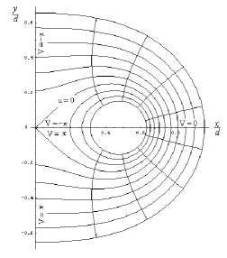
Figure 1: Equipotencial and field lines for the Coulombian equal charges (right semi-space). $V$ stands for $v/(2\,\lambda)$.

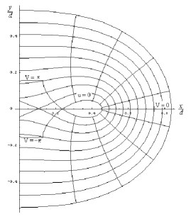
Figure 2: Multi-valued Born-Infeld mapping (29) for $-\pi<v/(2\,\lambda)<\pi$ ($\alpha^{2}=40$). In the figure $V$ stands for $v/(2\,\lambda)$.

Figure 3: Curves $|p(w)|=(2b)^{-1}$ characterized by $\alpha=bd/\lambda$ for the configuration of two equal charges. Only the cusps, but not the lobes, belong to the branch of $w(z)$ under consideration.

In order to compute the force (24) we will take into account that the points on the $y$-axis satisfy

$$\frac{u}{2\lambda}\,\;<\;\,0\,\,\,\,\;\quad\,\mbox{and}\,\,\quad\,\,\,\frac{v}{2\lambda}=\pm\pi.$$ (32)

Then, according to Eq.(29), the positive $y$-semiaxis can be parametrized by defining a parameter $t$ such that $\cos(t/2)=\exp[u/(4\lambda)]$; thus it results

$$y(t)=-\frac{d}{2}\;\,\left[{\tan\,{\frac{t}{2}}\;-\;\frac{4}{\alpha^{2}}\;\,(\pi+t-\sin\;t)}\right]$$ (33)

where $t\in(-\pi,t_{o})$. Then the integral (24) can be computed as twice the integral along the positive $y$ semi-axis. Thus the force is

$$F^{x}=\frac{2\lambda}{\pi\,d}\int\limits_{-\infty}^{\;\;\quad u_{o}}{\;\exp\left[{\frac{u}{2\lambda}}\right]\;\;\sqrt{\exp\left[{-\frac{u}{2\lambda}}\right]-1}\;\,du\,}$$

$$=\,\;\frac{4\lambda^{2}}{\pi\,d}\int\limits_{-\pi}^{\,\,\,\,\,\,\,t_{0}}{\sin^{2}\,{\frac{t}{2}}\,}dt\,=\;\,\,\frac{2\,\lambda^{2}}{\pi\,d}\;\left({\pi+t_{o}-\sin\,t_{o}}\right)\,$$ (34)

In the former expression, $u_{o}$ is such that $y(u_{o})=0$. In the Coulombian case ($b\to\infty$, i.e. $\alpha\to\infty$) it is $u_{o}=0$, so $t_{o}=0$ and the Coulomb force is recovered. Instead, in Born-Infeld theory it is $u_{o}<0$ and $-\pi<t_{o}<0$. The dependence of the interaction on $b$ is given through the value $t_{o}$ which depends on $\alpha=bd/\lambda$. Since $t_{o}-\sin t_{o}$ is negative for $-\pi<t_{o}<0$, it is concluded that the interaction between equal monopoles is repulsive for all value of $\alpha$, but less intense than the Coulombian interaction. In particular, for $\alpha\to 0$, it is $t_{o}\to-\pi$; thus the repulsive interaction force vanishes for $d\to 0$.

In order to get an explicit correction to the Coulombian force we will take into account that $t_{o}$ is small for high values of $\alpha$. Thus we can try to solve $y(t_{o})=0$ in (33) by writing $t_{o}$ as a power series of $\alpha^{-2}$. In this way we reach the result $t_{o}=-8\,\pi\,\alpha^{-2}+128\,\pi^{3}\,\alpha^{-6}/3-2048\,\pi^{3}\,\alpha^{-8}/3+O(\alpha^{-10})$. Therefore the force (34) is

$$F^{x}\;\;\mathrel{\mathop{\kern 0.0pt\longrightarrow}\limits_{\alpha\to\infty}}\;\,\frac{2\lambda^{2}}{d}\;\left({\,1-\;\,\frac{256\;\pi^{2}}{3\;\alpha^{6}}}\right)\,+\,O\mbox{(}\alpha^{-10}\mbox{)}.$$ (35)

Then, Born-Infeld correction to the repulsive force between equal charges is very weak. Notice that $d$ in (35) is not the real distance $D$ between the charges. $D$ goes to $d$ when $b\to\infty$, but $D$ is smaller than $d$ for equal charges (see Figure 3):

$$D_{repulsive}\,=\,d\,-\,\frac{2\,d}{\alpha^{2}}\,\left(\ln(\alpha^{2})-1\right)\,+\,O[\alpha^{-4}]\ .$$ (36)

IV.2 Opposite charges

We will now repeat the former steps for the case of the attractive charge configuration consisting of a charge $-\lambda$ at $x=-d/2$, and a charge $\lambda$ at $x=d/2$. The complex Coulombian potential is

$$w=-2\lambda\,\ln\left({\frac{\frac{2z}{d}-1}{\frac{2z}{d}+1}}\right).$$ (37)

Here we have chosen the integration constant such that $w(z)$ is null at infinity. Inverting (37) we obtain the Coulombian mapping

$$z\ =\ \frac{d}{2}\,\coth\,{\frac{w}{4\lambda}}\ ,$$ (38)

This means that function $p(w)$ is

$$p(w)=-\frac{d}{8\,\lambda}\,\sinh^{-2}\frac{w}{4\,\lambda}.$$ (39)

Thus the Born-Infeld mapping results

$$z=\frac{d}{2}\left[{\coth\,{\frac{w}{4\lambda}}+\frac{4}{\alpha^{2}}\left({\frac{\overline{w}}{2\lambda}-\sinh\,{\frac{\overline{w}}{2\lambda}}}\right)}\right].$$ (40)

The points where the electrostatic field reaches the value $b$ (i.e., $|p(w)|=(2\,b)^{-1}$) belong to the curve

$$\frac{u}{2\lambda}=\pm\;{\rm arccosh}\,\left({\frac{\alpha}{2}+\cos\,{\frac{v}{2\lambda}}}\right).$$ (41)

If $\alpha>4$ this curve decomposes in two separate parts (“charges”) at each side of the $y$-axis. Like the previous case, the Born-Infeld mapping (40) fails to be periodic due to the presence of a linear term; so the $u-v$ domain in mapping (40) should be properly restricted to get a single-valued potential $u(x,y)$. The branch of the complex potential $w$ to be kept is those matching the Coulombian potential at infinity. Differing from the previous case, this branch does reach the curves (41). Figures 4 and 5 show the equipotential ($u=constant$) and field ($v=constant$) lines surrounding the right charge, and their relation with curve (41). Again the lines $v=0$ coincide with the piece of the $x$-axis going between the charges and infinity. But in this case the domain of $|v|/(2\,\lambda)$ has to be extended beyond $\pi$ to reach the piece of the $x$-axis joining the charges. Both the potential $u$ and the field $\bf E$ are discontinuous at the charge (the field attains the maximum value $b$ at the exterior side of the charge, i.e. the side where $0\leq|v|/(2\,\lambda)\leq\pi$). Besides, the field is discontinuous at the branch cut on the $x$-axis between the charges.

For $\alpha\leq 4$ the curve of maximum field get closed, as it is typical for a dipole 21 . In this case, the “charge” distribution becomes a unique object; the Coulombian zone $|p(w)|>(2b)^{-1}$ is, of course, the outside of the object. Figure 6 shows the curves $|p(w)|=(2b)^{-1}$ for different values of $\alpha$. The curves display cusps on the $x$-axis ($v=0$) at $|x|>d/2$. At the cups it is $u=\pm 2\lambda\;{\rm arccosh}\,(\alpha/2+1)$.

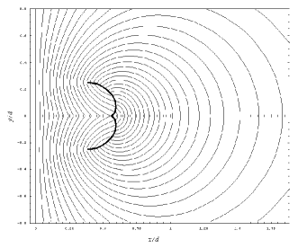
Figure 4: Born-Infeld equipotencial lines ($u=constant$) for $\alpha=5$, together with the curve describing the right charge.

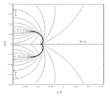
Figure 5: Born-Infeld field lines ($v=constant$) for $\alpha=5$, together with the curve describing the right charge. In the figure $V$ stands for $v/(2\,\lambda)$.

Figure 6: Born-Infeld opposite “charges” for $\alpha=10$ and $\alpha=5$. For $\alpha\leq 4$ the charges merge in a sole object.

We will calculate the force (25) for $\alpha>4$, which is the case where the charges are separate. Since the $y$-axis is characterized by $u=0$, then Eq.(40) says that the positive $y$-axis accepts a parametrization similar to (33) whenever the parameter $t$ is defined as $t=v/(2\lambda)-\pi$:

$$y(t)\ =\ -\frac{d}{2}\,\left[\tan\frac{t}{2}-\frac{4}{\alpha^{2}}(\pi+t+\sin t)\right]$$ (42)

This function is monotonous for $t\in(-\pi,t_{o})$, where $0<t_{o}<\pi$ is the parameter satisfying $y(t_{o})=0$. Since $p(w)|_{y-axis}=d/(8\lambda)\,\,\sin^{-2}\left[{v/(4\lambda)}\right]$, then the force (25) is

$$F^{x}=-\frac{4\,\lambda^{2}}{\pi\,d}\int\limits_{-\pi}^{t_{o}}{\cos^{\,2}\frac{t}{2}\,dt}=-\,\frac{2\,\lambda^{2}}{\pi\,d}\,(\pi+t_{o}+\sin\,t_{o})$$ (43)

For $b\to\infty$ ($\alpha\to\infty$), it is $t_{o}\to 0$ in Eq.(43), so the Coulombian force is recovered. Since $t_{o}\in(0,\pi)$, it is concluded that the attraction between opposite monopoles is more intense than Coulombian interaction. We will solve $y(t_{o})=0$ in (42) by writing $t_{o}$ as a power series of $(\alpha^{2}-16)^{-1}$. The result is $t_{o}=8\pi\,(\alpha^{2}-16)^{-1}\,(1-16\pi^{2}(\alpha^{2}-16)^{-2}/3)+O[(\alpha^{2}-16)^{-4}]$. Therefore the Born-Infeld interaction (43) between opposite monopoles behaves as

$$F^{x}\;\;\mathrel{\mathop{\kern 0.0pt\longrightarrow}\limits_{\alpha\to\infty}}\,\frac{2\lambda^{2}}{d}\,\left({1\,+\,\frac{16}{\alpha^{2}-16}-\,\frac{512\,\pi^{2}}{3(\alpha^{2}-16)^{3}}}\right)$$

$$+\,O\left[(\alpha^{2}-16)^{-4}\right].$$ (44)

Differing from the repulsive case, the attractive interaction receives a more perceptible correction of order $(\alpha^{2}-16)^{-1}$. Notice that $d$ in (IV.2) is not the distance $D$ between the cusps in Figure 6. By computing the positions of the cusps for opposite charges, it results that $D$ is larger than $d$:

$$D_{attractive}\,=\,d\,+\,\frac{2\,d}{\alpha^{2}-16}\,\left(\ln(\alpha^{2}-16)\,-\,3\right)$$

$$+\,O[(\alpha^{2}-16)^{-3/2}]\ .$$ (45)

V Conclusions

The first goal of Born-Infeld theory was the obtaining of a point-like charge solution with finite self-energy. However this solution has intriguing features: $\partial L_{BI}/\partial{\bf E}$ still diverges, and $\bf E$ is finite at the charge position (an unpleasant property for a vector field at its center of symmetry). However, these disagreeable features do not cause any trouble to the interaction between charges. We have considered a “two charges” field (which differs from the mere superposition of two “one charge” fields, since the theory is nonlinear). To compute the interaction between parts of this field configuration one must consider the momentum flux through a surface separating both subsystems. According to the method developed in Ref. 21 , the interaction force is given by expressions (17-18), where $p$ is a Coulombian function, and the Born-Infeld features are encoded in the integration interval. Although we have obtained the force in a parametric form (the parameter $t_{o}$ in forces (34) and (43) comes from the transcendent equation $y(t_{o})=0$ in (33) and (42) respectively), we have succeeded in computing Born-Infeld corrections to Coulombian interactions. In addition we have proved that the interaction force between equal charges is well behaved and goes to zero when the charges approach. This limit cannot be reached for opposite charges because they merge in a unique dipolar object of finite size.

- (1) M. Born, L. Infeld, Nature 132, 1004 (1933).
- (2) M. Born, L. Infeld, Proc. Roy. Soc. A 144, 425 (1934).
- (3) M. Born, L. Infeld, Proc. Roy. Soc. A 147, 522 (1934).
- (4) M. Born, L. Infeld, Proc. Roy. Soc. A 150, 141 (1935).
- (5) B.Hoffman, L. Infeld, Phys. Rev. 51, 765 (1937).
- (6) J. Plebanski, Lectures on non linear electrodynamics, Nordita Lecture Notes, Nordita: Copenhagen, 1968.
- (7) S. Deser, R. Puzalowski, J. Phys. A 13, 2501 (1980).
- (8) G. Boillat, J. Math. Phys. 11, 941 (1970).
- (9) M. Aiello, G.R. Bengochea and R. Ferraro, Phys. Lett. A 361 9 (2007).
- (10) R. Ferraro, Phys. Rev. Lett. 99, 230401 (2007).
- (11) A. Abouelsaood, C. Callan, C. Nappi and S. Yost, Nucl. Phys. B 280 (1987), 599.
- (12) R. Metsaev, M. Rahmanov, A. Tseytlin, Phys. Lett. B 193, 207 (1987).
- (13) A. Tseytlin, Nuc. Phys. B 501, 41 (1997).
- (14) V.V. Dyadichev, D.V. Gal tsov and A.G. Zorin, Phys. Rev. D 65, 084007 (2002); P. Vargas Moniz, Phys. Rev. D 66, 103501 (2002); M. Sami, N. Dadhich, and T. Shiromizu, Phys. Lett. B 568, 118 (2003).
- (15) D. Palatnik, Phys. Lett. B 432, 287 (1998); S. Deser and G.W. Gibbons, Class. Quantum Grav. 15, L35 (1998).
- (16) D. Wiltshire, Phys. Rev. D 38, 2445 (1998); Cai, R-G., Phys. Rev. D 63, 124018 (2001); M. Aiello, R. Ferraro, G. Giribet, Phys. Rev. D 70, 104014 (2004).
- (17) H. Bateman, Partial Differential Equations of Mathematical Physics, Dover: N.Y., 1944.
- (18) A. R. Forsyth, A Treatise of Differential Equations, McMillan: London, 1956.
- (19) M. H. L. Pryce, Proc. Cambr. Phil. Soc. 31, 625 (1935).
- (20) M. H. L. Pryce, Proc. Cambr. Phil. Soc. 31, 50 (1935).
- (21) R. Ferraro, Phys. Lett. A 325, 134 (2004).
- (22) Z. Nehari, Conformal Mapping, McGraw-Hill, 1952.
- (23) P.M. Morse, H. Feshbach, Methods of Theoretical Physics, Vol. 2, McGraw-Hill: N.Y., 1953.
- (24) R. Churchill, J. Brown, Complex Variables and Applications, McGraw-Hill: N.Y., 1984.