Orbit Spaces of Compact Linear Groups

Abstract

The $\widehat{P}$-matrix approach for the determination of the orbit spaces of compact linear groups enabled to determine all orbit spaces of compact coregular linear groups with up to 4 basic polynomial invariants and, more recently, all orbit spaces of compact non-coregular linear groups with up to 3 basic invariants. This approach does not involve the knowledge of the group structure of the single groups but it is very general, so after the determination of the orbit spaces one has to determine the corresponding groups. In this article it is reviewed the main ideas underlying the $\widehat{P}$-matrix approach and it is reported the list of linear irreducible finite groups and of linear compact simple Lie groups, with up to 4 basic invariants, together with their orbit spaces. Some general properties of orbit spaces of coregular groups are also discussed. This article will deal only with the mathematical aspect, however one must keep in mind that the stratification of the orbit spaces represents the possible schemes of symmetry breaking and that the phase transitions appear when the minimum of an invariant potential function shifts from one stratum to another, so the exact knowledge of the orbit spaces and their stratifications might be useful to single out some yet hidden properties of phase transitions.

1 Basic Definitions on Compact Group Actions

In this article it will be given only a short survey on the determination of orbit spaces of compact linear groups. More details can be found in [1, 2, 3].

When a physical system has to show a symmetry of the nature, it must be described mathematically on a certain representation space of a group $G$ in such a way that all physically relevant quantities are invariant with respect to $G$-transformations.
Often the group $G$ is compact and its representation space is finite dimensional. In this case in all generality one might suppose that $G$ is a group of real orthogonal matrices acting on the real vector space ${\mathchoice{\hbox{$\displaystyle\kern-0.56905pt1\kern-2.84526pt\mbox{\rm R}\kern-0.56905pt$}}{\hbox{$\textstyle\kern-0.56905pt1\kern-2.84526pt\mbox{\rm R}\kern-0.56905pt$}}{\hbox{$\scriptstyle\kern-0.56905pt1\kern-2.84526pt\mbox{\rm R}\kern-0.56905pt$}}{\hbox{$\scriptscriptstyle\kern-0.56905pt1\kern-2.84526pt\mbox{\rm R}\kern-0.56905pt$}}}^{n}$. In the following it will be assumed that $G\subseteq O(n)$ and also that the origin of ${\mathchoice{\hbox{$\displaystyle\kern-0.56905pt1\kern-2.84526pt\mbox{\rm R}\kern-0.56905pt$}}{\hbox{$\textstyle\kern-0.56905pt1\kern-2.84526pt\mbox{\rm R}\kern-0.56905pt$}}{\hbox{$\scriptstyle\kern-0.56905pt1\kern-2.84526pt\mbox{\rm R}\kern-0.56905pt$}}{\hbox{$\scriptscriptstyle\kern-0.56905pt1\kern-2.84526pt\mbox{\rm R}\kern-0.56905pt$}}}^{n}$ is the only point left fixed by all transformations of $G$.

The orbit through $x\in{\mathchoice{\hbox{$\displaystyle\kern-0.56905pt1\kern-2.84526pt\mbox{\rm R}\kern-0.56905pt$}}{\hbox{$\textstyle\kern-0.56905pt1\kern-2.84526pt\mbox{\rm R}\kern-0.56905pt$}}{\hbox{$\scriptstyle\kern-0.56905pt1\kern-2.84526pt\mbox{\rm R}\kern-0.56905pt$}}{\hbox{$\scriptscriptstyle\kern-0.56905pt1\kern-2.84526pt\mbox{\rm R}\kern-0.56905pt$}}}^{n}$ is the subset of ${\mathchoice{\hbox{$\displaystyle\kern-0.56905pt1\kern-2.84526pt\mbox{\rm R}\kern-0.56905pt$}}{\hbox{$\textstyle\kern-0.56905pt1\kern-2.84526pt\mbox{\rm R}\kern-0.56905pt$}}{\hbox{$\scriptstyle\kern-0.56905pt1\kern-2.84526pt\mbox{\rm R}\kern-0.56905pt$}}{\hbox{$\scriptscriptstyle\kern-0.56905pt1\kern-2.84526pt\mbox{\rm R}\kern-0.56905pt$}}}^{n}$ formed by all points connected to $x$ by $G$-transformations:

$$\Omega(x)=\{g\cdot x,\quad\forall g\in G\},\qquad x\in{\mathchoice{\hbox{$\displaystyle\kern-0.56905pt1\kern-2.84526pt\mbox{\rm R}\kern-0.56905pt$}}{\hbox{$\textstyle\kern-0.56905pt1\kern-2.84526pt\mbox{\rm R}\kern-0.56905pt$}}{\hbox{$\scriptstyle\kern-0.56905pt1\kern-2.84526pt\mbox{\rm R}\kern-0.56905pt$}}{\hbox{$\scriptscriptstyle\kern-0.56905pt1\kern-2.84526pt\mbox{\rm R}\kern-0.56905pt$}}}^{n}$$

The isotropy subgroup $G_{x}$ of the point $x$ is the subgroup of $G$ that leaves $x$ fixed:

$$G_{x}=\{g\in G\mid g\cdot x=x\},\qquad x\in{\mathchoice{\hbox{$\displaystyle\kern-0.56905pt1\kern-2.84526pt\mbox{\rm R}\kern-0.56905pt$}}{\hbox{$\textstyle\kern-0.56905pt1\kern-2.84526pt\mbox{\rm R}\kern-0.56905pt$}}{\hbox{$\scriptstyle\kern-0.56905pt1\kern-2.84526pt\mbox{\rm R}\kern-0.56905pt$}}{\hbox{$\scriptscriptstyle\kern-0.56905pt1\kern-2.84526pt\mbox{\rm R}\kern-0.56905pt$}}}^{n}$$

All the points in a same orbit $\Omega(x)$ have isotropy subgroups in a same conjugacy class $[G_{x}]$ of subgroups of $G$, called the orbit type of $\Omega(x)$, in fact one has:

$$G_{g\cdot x}=g\cdot G_{x}\cdot g^{-1},\qquad\forall g\in G,\qquad x\in{\mathchoice{\hbox{$\displaystyle\kern-0.56905pt1\kern-2.84526pt\mbox{\rm R}\kern-0.56905pt$}}{\hbox{$\textstyle\kern-0.56905pt1\kern-2.84526pt\mbox{\rm R}\kern-0.56905pt$}}{\hbox{$\scriptstyle\kern-0.56905pt1\kern-2.84526pt\mbox{\rm R}\kern-0.56905pt$}}{\hbox{$\scriptscriptstyle\kern-0.56905pt1\kern-2.84526pt\mbox{\rm R}\kern-0.56905pt$}}}^{n}$$

To each orbit type $[H]$ it is associated a stratum $\Sigma_{[H]}$, formed by all points of ${\mathchoice{\hbox{$\displaystyle\kern-0.56905pt1\kern-2.84526pt\mbox{\rm R}\kern-0.56905pt$}}{\hbox{$\textstyle\kern-0.56905pt1\kern-2.84526pt\mbox{\rm R}\kern-0.56905pt$}}{\hbox{$\scriptstyle\kern-0.56905pt1\kern-2.84526pt\mbox{\rm R}\kern-0.56905pt$}}{\hbox{$\scriptscriptstyle\kern-0.56905pt1\kern-2.84526pt\mbox{\rm R}\kern-0.56905pt$}}}^{n}$ that have isotropy subgroups in $[H]$:

$$\Sigma_{[H]}=\{x\in{\mathchoice{\hbox{$\displaystyle\kern-0.56905pt1\kern-2.84526pt\mbox{\rm R}\kern-0.56905pt$}}{\hbox{$\textstyle\kern-0.56905pt1\kern-2.84526pt\mbox{\rm R}\kern-0.56905pt$}}{\hbox{$\scriptstyle\kern-0.56905pt1\kern-2.84526pt\mbox{\rm R}\kern-0.56905pt$}}{\hbox{$\scriptscriptstyle\kern-0.56905pt1\kern-2.84526pt\mbox{\rm R}\kern-0.56905pt$}}}^{n}\mid G_{x}\in[H]\}$$

The orbits (and the strata) are disjoint subsets of ${\mathchoice{\hbox{$\displaystyle\kern-0.56905pt1\kern-2.84526pt\mbox{\rm R}\kern-0.56905pt$}}{\hbox{$\textstyle\kern-0.56905pt1\kern-2.84526pt\mbox{\rm R}\kern-0.56905pt$}}{\hbox{$\scriptstyle\kern-0.56905pt1\kern-2.84526pt\mbox{\rm R}\kern-0.56905pt$}}{\hbox{$\scriptscriptstyle\kern-0.56905pt1\kern-2.84526pt\mbox{\rm R}\kern-0.56905pt$}}}^{n}$, as each orbit has one and only one orbit type.
The orbits and the strata can be partially ordered according to their orbit types [H]. The orbit type $[H]$ is said to be smaller than the orbit type $[K]$: $[H]<[K]$, if $H^{\prime}\subset K^{\prime}$ for some $H^{\prime}\in[H]$ and $K^{\prime}\in[K]$. Then $[K]$ is greater than $[H]$.

Due to the compactness of $G$, the number of different orbit types is finite and there is a unique minimal orbit type. The unique stratum of smallest orbit type is called the principal stratum. All other strata are called singular.

The orbit space is the quotient space ${\mathchoice{\hbox{$\displaystyle\kern-0.56905pt1\kern-2.84526pt\mbox{\rm R}\kern-0.56905pt$}}{\hbox{$\textstyle\kern-0.56905pt1\kern-2.84526pt\mbox{\rm R}\kern-0.56905pt$}}{\hbox{$\scriptstyle\kern-0.56905pt1\kern-2.84526pt\mbox{\rm R}\kern-0.56905pt$}}{\hbox{$\scriptscriptstyle\kern-0.56905pt1\kern-2.84526pt\mbox{\rm R}\kern-0.56905pt$}}}^{n}/G$ defined through the equivalence relation relating points belonging to the same orbit. The natural projection $\pi:{\mathchoice{\hbox{$\displaystyle\kern-0.56905pt1\kern-2.84526pt\mbox{\rm R}\kern-0.56905pt$}}{\hbox{$\textstyle\kern-0.56905pt1\kern-2.84526pt\mbox{\rm R}\kern-0.56905pt$}}{\hbox{$\scriptstyle\kern-0.56905pt1\kern-2.84526pt\mbox{\rm R}\kern-0.56905pt$}}{\hbox{$\scriptscriptstyle\kern-0.56905pt1\kern-2.84526pt\mbox{\rm R}\kern-0.56905pt$}}}^{n}\to{\mathchoice{\hbox{$\displaystyle\kern-0.56905pt1\kern-2.84526pt\mbox{\rm R}\kern-0.56905pt$}}{\hbox{$\textstyle\kern-0.56905pt1\kern-2.84526pt\mbox{\rm R}\kern-0.56905pt$}}{\hbox{$\scriptstyle\kern-0.56905pt1\kern-2.84526pt\mbox{\rm R}\kern-0.56905pt$}}{\hbox{$\scriptscriptstyle\kern-0.56905pt1\kern-2.84526pt\mbox{\rm R}\kern-0.56905pt$}}}^{n}/G$ maps the orbits of ${\mathchoice{\hbox{$\displaystyle\kern-0.56905pt1\kern-2.84526pt\mbox{\rm R}\kern-0.56905pt$}}{\hbox{$\textstyle\kern-0.56905pt1\kern-2.84526pt\mbox{\rm R}\kern-0.56905pt$}}{\hbox{$\scriptstyle\kern-0.56905pt1\kern-2.84526pt\mbox{\rm R}\kern-0.56905pt$}}{\hbox{$\scriptscriptstyle\kern-0.56905pt1\kern-2.84526pt\mbox{\rm R}\kern-0.56905pt$}}}^{n}$ into single points of ${\mathchoice{\hbox{$\displaystyle\kern-0.56905pt1\kern-2.84526pt\mbox{\rm R}\kern-0.56905pt$}}{\hbox{$\textstyle\kern-0.56905pt1\kern-2.84526pt\mbox{\rm R}\kern-0.56905pt$}}{\hbox{$\scriptstyle\kern-0.56905pt1\kern-2.84526pt\mbox{\rm R}\kern-0.56905pt$}}{\hbox{$\scriptscriptstyle\kern-0.56905pt1\kern-2.84526pt\mbox{\rm R}\kern-0.56905pt$}}}^{n}/G$. Projections of strata of ${\mathchoice{\hbox{$\displaystyle\kern-0.56905pt1\kern-2.84526pt\mbox{\rm R}\kern-0.56905pt$}}{\hbox{$\textstyle\kern-0.56905pt1\kern-2.84526pt\mbox{\rm R}\kern-0.56905pt$}}{\hbox{$\scriptstyle\kern-0.56905pt1\kern-2.84526pt\mbox{\rm R}\kern-0.56905pt$}}{\hbox{$\scriptscriptstyle\kern-0.56905pt1\kern-2.84526pt\mbox{\rm R}\kern-0.56905pt$}}}^{n}$ define strata of ${\mathchoice{\hbox{$\displaystyle\kern-0.56905pt1\kern-2.84526pt\mbox{\rm R}\kern-0.56905pt$}}{\hbox{$\textstyle\kern-0.56905pt1\kern-2.84526pt\mbox{\rm R}\kern-0.56905pt$}}{\hbox{$\scriptstyle\kern-0.56905pt1\kern-2.84526pt\mbox{\rm R}\kern-0.56905pt$}}{\hbox{$\scriptscriptstyle\kern-0.56905pt1\kern-2.84526pt\mbox{\rm R}\kern-0.56905pt$}}}^{n}/G$. The principal stratum of ${\mathchoice{\hbox{$\displaystyle\kern-0.56905pt1\kern-2.84526pt\mbox{\rm R}\kern-0.56905pt$}}{\hbox{$\textstyle\kern-0.56905pt1\kern-2.84526pt\mbox{\rm R}\kern-0.56905pt$}}{\hbox{$\scriptstyle\kern-0.56905pt1\kern-2.84526pt\mbox{\rm R}\kern-0.56905pt$}}{\hbox{$\scriptscriptstyle\kern-0.56905pt1\kern-2.84526pt\mbox{\rm R}\kern-0.56905pt$}}}^{n}/G$ is always open connected and dense in ${\mathchoice{\hbox{$\displaystyle\kern-0.56905pt1\kern-2.84526pt\mbox{\rm R}\kern-0.56905pt$}}{\hbox{$\textstyle\kern-0.56905pt1\kern-2.84526pt\mbox{\rm R}\kern-0.56905pt$}}{\hbox{$\scriptstyle\kern-0.56905pt1\kern-2.84526pt\mbox{\rm R}\kern-0.56905pt$}}{\hbox{$\scriptscriptstyle\kern-0.56905pt1\kern-2.84526pt\mbox{\rm R}\kern-0.56905pt$}}}^{n}/G$, so also ${\mathchoice{\hbox{$\displaystyle\kern-0.56905pt1\kern-2.84526pt\mbox{\rm R}\kern-0.56905pt$}}{\hbox{$\textstyle\kern-0.56905pt1\kern-2.84526pt\mbox{\rm R}\kern-0.56905pt$}}{\hbox{$\scriptstyle\kern-0.56905pt1\kern-2.84526pt\mbox{\rm R}\kern-0.56905pt$}}{\hbox{$\scriptscriptstyle\kern-0.56905pt1\kern-2.84526pt\mbox{\rm R}\kern-0.56905pt$}}}^{n}/G$ is connected. If $[K]>[H]$, then $\pi(\Sigma_{[K]})$ lies in the boundary of $\pi(\Sigma_{[H]})$, so to greater orbit types correspond strata of smaller dimension and the boundary of the principal stratum contains all singular strata. Clearly there is a one to one correspondence between the strata of ${\mathchoice{\hbox{$\displaystyle\kern-0.56905pt1\kern-2.84526pt\mbox{\rm R}\kern-0.56905pt$}}{\hbox{$\textstyle\kern-0.56905pt1\kern-2.84526pt\mbox{\rm R}\kern-0.56905pt$}}{\hbox{$\scriptstyle\kern-0.56905pt1\kern-2.84526pt\mbox{\rm R}\kern-0.56905pt$}}{\hbox{$\scriptscriptstyle\kern-0.56905pt1\kern-2.84526pt\mbox{\rm R}\kern-0.56905pt$}}}^{n}$ and the strata of ${\mathchoice{\hbox{$\displaystyle\kern-0.56905pt1\kern-2.84526pt\mbox{\rm R}\kern-0.56905pt$}}{\hbox{$\textstyle\kern-0.56905pt1\kern-2.84526pt\mbox{\rm R}\kern-0.56905pt$}}{\hbox{$\scriptstyle\kern-0.56905pt1\kern-2.84526pt\mbox{\rm R}\kern-0.56905pt$}}{\hbox{$\scriptscriptstyle\kern-0.56905pt1\kern-2.84526pt\mbox{\rm R}\kern-0.56905pt$}}}^{n}/G$, so ${\mathchoice{\hbox{$\displaystyle\kern-0.56905pt1\kern-2.84526pt\mbox{\rm R}\kern-0.56905pt$}}{\hbox{$\textstyle\kern-0.56905pt1\kern-2.84526pt\mbox{\rm R}\kern-0.56905pt$}}{\hbox{$\scriptstyle\kern-0.56905pt1\kern-2.84526pt\mbox{\rm R}\kern-0.56905pt$}}{\hbox{$\scriptscriptstyle\kern-0.56905pt1\kern-2.84526pt\mbox{\rm R}\kern-0.56905pt$}}}^{n}$ and ${\mathchoice{\hbox{$\displaystyle\kern-0.56905pt1\kern-2.84526pt\mbox{\rm R}\kern-0.56905pt$}}{\hbox{$\textstyle\kern-0.56905pt1\kern-2.84526pt\mbox{\rm R}\kern-0.56905pt$}}{\hbox{$\scriptstyle\kern-0.56905pt1\kern-2.84526pt\mbox{\rm R}\kern-0.56905pt$}}{\hbox{$\scriptscriptstyle\kern-0.56905pt1\kern-2.84526pt\mbox{\rm R}\kern-0.56905pt$}}}^{n}/G$ are stratified in exactly the same manner.

For all the $G$-invariant functions, $f(g\cdot x)=f(x),\ \forall g\in G,\ x\in{\mathchoice{\hbox{$\displaystyle\kern-0.56905pt1\kern-2.84526pt\mbox{\rm R}\kern-0.56905pt$}}{\hbox{$\textstyle\kern-0.56905pt1\kern-2.84526pt\mbox{\rm R}\kern-0.56905pt$}}{\hbox{$\scriptstyle\kern-0.56905pt1\kern-2.84526pt\mbox{\rm R}\kern-0.56905pt$}}{\hbox{$\scriptscriptstyle\kern-0.56905pt1\kern-2.84526pt\mbox{\rm R}\kern-0.56905pt$}}}^{n}$, so the invariant functions are constant on the orbits. Then can then be thought as functions defined on the orbit space and in this way one eliminates the degeneration of all the points belonging to a same orbit, in which $f(x)$ is constant.
The isotropy subgroup of the minimum point of an invariant potential function determines the true symmetry group of a physical system and if this minimum is not at the origin then one has a symmetry breaking.

The potential may depend on some variable parameters, so the location of the minimum point also depends on these parameters and a phase transition is realized when the minimum point changes stratum. Keeping these things in mind one may realize that many properties of invariant functions and phase transitions can be better studied in the orbit spaces.

2 Orbit Spaces in ${\mathchoice{\hbox{$\displaystyle\kern-0.56905pt1\kern-2.84526pt\mbox{\rm R}\kern-0.56905pt$}}{\hbox{$\textstyle\kern-0.56905pt1\kern-2.84526pt\mbox{\rm R}\kern-0.56905pt$}}{\hbox{$\scriptstyle\kern-0.56905pt1\kern-2.84526pt\mbox{\rm R}\kern-0.56905pt$}}{\hbox{$\scriptscriptstyle\kern-0.56905pt1\kern-2.84526pt\mbox{\rm R}\kern-0.56905pt$}}}^{q}$ and $\widehat{P}$-matrices

A concrete mathematical description of the orbit space is achieved through an integrity basis (IB) $\ p_{1}(x),\ldots,p_{q}(x)\$ for the ring $\ {\mathchoice{\hbox{$\displaystyle\kern-0.56905pt1\kern-2.84526pt\mbox{\rm R}\kern-0.56905pt$}}{\hbox{$\textstyle\kern-0.56905pt1\kern-2.84526pt\mbox{\rm R}\kern-0.56905pt$}}{\hbox{$\scriptstyle\kern-0.56905pt1\kern-2.84526pt\mbox{\rm R}\kern-0.56905pt$}}{\hbox{$\scriptscriptstyle\kern-0.56905pt1\kern-2.84526pt\mbox{\rm R}\kern-0.56905pt$}}}[{\mathchoice{\hbox{$\displaystyle\kern-0.56905pt1\kern-2.84526pt\mbox{\rm R}\kern-0.56905pt$}}{\hbox{$\textstyle\kern-0.56905pt1\kern-2.84526pt\mbox{\rm R}\kern-0.56905pt$}}{\hbox{$\scriptstyle\kern-0.56905pt1\kern-2.84526pt\mbox{\rm R}\kern-0.56905pt$}}{\hbox{$\scriptscriptstyle\kern-0.56905pt1\kern-2.84526pt\mbox{\rm R}\kern-0.56905pt$}}}^{n}]^{G}\$ of the $G$-invariant polynomial functions defined on ${\mathchoice{\hbox{$\displaystyle\kern-0.56905pt1\kern-2.84526pt\mbox{\rm R}\kern-0.56905pt$}}{\hbox{$\textstyle\kern-0.56905pt1\kern-2.84526pt\mbox{\rm R}\kern-0.56905pt$}}{\hbox{$\scriptstyle\kern-0.56905pt1\kern-2.84526pt\mbox{\rm R}\kern-0.56905pt$}}{\hbox{$\scriptscriptstyle\kern-0.56905pt1\kern-2.84526pt\mbox{\rm R}\kern-0.56905pt$}}}^{n}$. All $G$-invariant polynomial (or $C^{\infty}$) functions can be expressed as polynomials (or $C^{\infty}$) functions of the finite number $q$ of basic polynomial invariant functions forming the IB:

$$f(x)=\widehat{f}(p_{1}(x),\ldots,p_{q}(x)),\qquad\forall f\in{\mathchoice{\hbox{$\displaystyle\kern-0.56905pt1\kern-2.84526pt\mbox{\rm R}\kern-0.56905pt$}}{\hbox{$\textstyle\kern-0.56905pt1\kern-2.84526pt\mbox{\rm R}\kern-0.56905pt$}}{\hbox{$\scriptstyle\kern-0.56905pt1\kern-2.84526pt\mbox{\rm R}\kern-0.56905pt$}}{\hbox{$\scriptscriptstyle\kern-0.56905pt1\kern-2.84526pt\mbox{\rm R}\kern-0.56905pt$}}}[{\mathchoice{\hbox{$\displaystyle\kern-0.56905pt1\kern-2.84526pt\mbox{\rm R}\kern-0.56905pt$}}{\hbox{$\textstyle\kern-0.56905pt1\kern-2.84526pt\mbox{\rm R}\kern-0.56905pt$}}{\hbox{$\scriptstyle\kern-0.56905pt1\kern-2.84526pt\mbox{\rm R}\kern-0.56905pt$}}{\hbox{$\scriptscriptstyle\kern-0.56905pt1\kern-2.84526pt\mbox{\rm R}\kern-0.56905pt$}}}^{n}]^{G}\qquad(\mbox{or}\ \forall f\in C^{\infty}[{\mathchoice{\hbox{$\displaystyle\kern-0.56905pt1\kern-2.84526pt\mbox{\rm R}\kern-0.56905pt$}}{\hbox{$\textstyle\kern-0.56905pt1\kern-2.84526pt\mbox{\rm R}\kern-0.56905pt$}}{\hbox{$\scriptstyle\kern-0.56905pt1\kern-2.84526pt\mbox{\rm R}\kern-0.56905pt$}}{\hbox{$\scriptscriptstyle\kern-0.56905pt1\kern-2.84526pt\mbox{\rm R}\kern-0.56905pt$}}}^{n}]^{G})$$

The IB is supposed minimal, i.e. no subset of the IB is itself an IB, and formed by homogeneous polynomial functions. The choice of the IB is not unique, but the group fixes the number $q$ of its elements and their degrees $d_{1},\ldots,d_{q}$.
We assume that the basic invariants $p_{i}(x)$ are labelled in such a way that $d_{i}\geq d_{i+1}$. As there are no fixed points except the origin of ${\mathchoice{\hbox{$\displaystyle\kern-0.56905pt1\kern-2.84526pt\mbox{\rm R}\kern-0.56905pt$}}{\hbox{$\textstyle\kern-0.56905pt1\kern-2.84526pt\mbox{\rm R}\kern-0.56905pt$}}{\hbox{$\scriptstyle\kern-0.56905pt1\kern-2.84526pt\mbox{\rm R}\kern-0.56905pt$}}{\hbox{$\scriptscriptstyle\kern-0.56905pt1\kern-2.84526pt\mbox{\rm R}\kern-0.56905pt$}}}^{n}$, $d_{q}\geq 2$, and, because of the orthogonality of $G$, we may take $\ p_{q}(x)=\sum_{i=1}^{n}x_{i}^{2}\$.

All IB transformations (IBTs):

$$p_{i}^{\prime}(x)=p_{i}^{\prime}(p_{1}(x),\ldots,p_{q}(x)),\qquad i=1,\ldots,q-1,\qquad p_{q}^{\prime}(x)=p_{q}(x)$$

that satisfy the conventions adopted must have Jacobian matrix with elements $J_{ij}(x)=\partial p_{i}^{\prime}(x)/\partial p_{j}(x)$ that are 0 or $G$-invariant homogeneous polynomial functions of degree: $\deg(J_{ij})=d_{i}-d_{j}$. Then, $J(x)$ is an upper block triangular matrix and $\det J(x)$ is a non vanishing constant.

The IB can be used to represent the orbits of ${\mathchoice{\hbox{$\displaystyle\kern-0.56905pt1\kern-2.84526pt\mbox{\rm R}\kern-0.56905pt$}}{\hbox{$\textstyle\kern-0.56905pt1\kern-2.84526pt\mbox{\rm R}\kern-0.56905pt$}}{\hbox{$\scriptstyle\kern-0.56905pt1\kern-2.84526pt\mbox{\rm R}\kern-0.56905pt$}}{\hbox{$\scriptscriptstyle\kern-0.56905pt1\kern-2.84526pt\mbox{\rm R}\kern-0.56905pt$}}}^{n}$ as points of ${\mathchoice{\hbox{$\displaystyle\kern-0.56905pt1\kern-2.84526pt\mbox{\rm R}\kern-0.56905pt$}}{\hbox{$\textstyle\kern-0.56905pt1\kern-2.84526pt\mbox{\rm R}\kern-0.56905pt$}}{\hbox{$\scriptstyle\kern-0.56905pt1\kern-2.84526pt\mbox{\rm R}\kern-0.56905pt$}}{\hbox{$\scriptscriptstyle\kern-0.56905pt1\kern-2.84526pt\mbox{\rm R}\kern-0.56905pt$}}}^{q}$. In fact, given an orbit $\Omega$, the vector function $(p_{1}(x),p_{2}(x),\ldots,p_{q}(x))\$is constant on $\Omega$, because the $p_{i}(x)$ are $G$-invariant. The $q$ numbers $p_{i}=p_{i}(x),\ x\in\Omega$, determine a point $p=(p_{1},p_{2},\ldots,p_{q})\in{\mathchoice{\hbox{$\displaystyle\kern-0.56905pt1\kern-2.84526pt\mbox{\rm R}\kern-0.56905pt$}}{\hbox{$\textstyle\kern-0.56905pt1\kern-2.84526pt\mbox{\rm R}\kern-0.56905pt$}}{\hbox{$\scriptstyle\kern-0.56905pt1\kern-2.84526pt\mbox{\rm R}\kern-0.56905pt$}}{\hbox{$\scriptscriptstyle\kern-0.56905pt1\kern-2.84526pt\mbox{\rm R}\kern-0.56905pt$}}}^{q}$, which can be considered the image in ${\mathchoice{\hbox{$\displaystyle\kern-0.56905pt1\kern-2.84526pt\mbox{\rm R}\kern-0.56905pt$}}{\hbox{$\textstyle\kern-0.56905pt1\kern-2.84526pt\mbox{\rm R}\kern-0.56905pt$}}{\hbox{$\scriptstyle\kern-0.56905pt1\kern-2.84526pt\mbox{\rm R}\kern-0.56905pt$}}{\hbox{$\scriptscriptstyle\kern-0.56905pt1\kern-2.84526pt\mbox{\rm R}\kern-0.56905pt$}}}^{q}$ of $\Omega$. No other orbit of ${\mathchoice{\hbox{$\displaystyle\kern-0.56905pt1\kern-2.84526pt\mbox{\rm R}\kern-0.56905pt$}}{\hbox{$\textstyle\kern-0.56905pt1\kern-2.84526pt\mbox{\rm R}\kern-0.56905pt$}}{\hbox{$\scriptstyle\kern-0.56905pt1\kern-2.84526pt\mbox{\rm R}\kern-0.56905pt$}}{\hbox{$\scriptscriptstyle\kern-0.56905pt1\kern-2.84526pt\mbox{\rm R}\kern-0.56905pt$}}}^{n}$ is represented in ${\mathchoice{\hbox{$\displaystyle\kern-0.56905pt1\kern-2.84526pt\mbox{\rm R}\kern-0.56905pt$}}{\hbox{$\textstyle\kern-0.56905pt1\kern-2.84526pt\mbox{\rm R}\kern-0.56905pt$}}{\hbox{$\scriptstyle\kern-0.56905pt1\kern-2.84526pt\mbox{\rm R}\kern-0.56905pt$}}{\hbox{$\scriptscriptstyle\kern-0.56905pt1\kern-2.84526pt\mbox{\rm R}\kern-0.56905pt$}}}^{q}$ by the same point because the IB separates the orbits.
The vector map:

$$p:{\mathchoice{\hbox{$\displaystyle\kern-0.56905pt1\kern-2.84526pt\mbox{\rm R}\kern-0.56905pt$}}{\hbox{$\textstyle\kern-0.56905pt1\kern-2.84526pt\mbox{\rm R}\kern-0.56905pt$}}{\hbox{$\scriptstyle\kern-0.56905pt1\kern-2.84526pt\mbox{\rm R}\kern-0.56905pt$}}{\hbox{$\scriptscriptstyle\kern-0.56905pt1\kern-2.84526pt\mbox{\rm R}\kern-0.56905pt$}}}^{n}\to{\mathchoice{\hbox{$\displaystyle\kern-0.56905pt1\kern-2.84526pt\mbox{\rm R}\kern-0.56905pt$}}{\hbox{$\textstyle\kern-0.56905pt1\kern-2.84526pt\mbox{\rm R}\kern-0.56905pt$}}{\hbox{$\scriptstyle\kern-0.56905pt1\kern-2.84526pt\mbox{\rm R}\kern-0.56905pt$}}{\hbox{$\scriptscriptstyle\kern-0.56905pt1\kern-2.84526pt\mbox{\rm R}\kern-0.56905pt$}}}^{q}:x\to(p_{1}(x),p_{2}(x),\ldots,p_{q}(x))$$

is called the orbit map. It maps ${\mathchoice{\hbox{$\displaystyle\kern-0.56905pt1\kern-2.84526pt\mbox{\rm R}\kern-0.56905pt$}}{\hbox{$\textstyle\kern-0.56905pt1\kern-2.84526pt\mbox{\rm R}\kern-0.56905pt$}}{\hbox{$\scriptstyle\kern-0.56905pt1\kern-2.84526pt\mbox{\rm R}\kern-0.56905pt$}}{\hbox{$\scriptscriptstyle\kern-0.56905pt1\kern-2.84526pt\mbox{\rm R}\kern-0.56905pt$}}}^{n}$ onto the subset ${\cal S}\subset{\mathchoice{\hbox{$\displaystyle\kern-0.56905pt1\kern-2.84526pt\mbox{\rm R}\kern-0.56905pt$}}{\hbox{$\textstyle\kern-0.56905pt1\kern-2.84526pt\mbox{\rm R}\kern-0.56905pt$}}{\hbox{$\scriptstyle\kern-0.56905pt1\kern-2.84526pt\mbox{\rm R}\kern-0.56905pt$}}{\hbox{$\scriptscriptstyle\kern-0.56905pt1\kern-2.84526pt\mbox{\rm R}\kern-0.56905pt$}}}^{q}$:

$${\cal S}=p({\mathchoice{\hbox{$\displaystyle\kern-0.56905pt1\kern-2.84526pt\mbox{\rm R}\kern-0.56905pt$}}{\hbox{$\textstyle\kern-0.56905pt1\kern-2.84526pt\mbox{\rm R}\kern-0.56905pt$}}{\hbox{$\scriptstyle\kern-0.56905pt1\kern-2.84526pt\mbox{\rm R}\kern-0.56905pt$}}{\hbox{$\scriptscriptstyle\kern-0.56905pt1\kern-2.84526pt\mbox{\rm R}\kern-0.56905pt$}}}^{n})\subset{\mathchoice{\hbox{$\displaystyle\kern-0.56905pt1\kern-2.84526pt\mbox{\rm R}\kern-0.56905pt$}}{\hbox{$\textstyle\kern-0.56905pt1\kern-2.84526pt\mbox{\rm R}\kern-0.56905pt$}}{\hbox{$\scriptstyle\kern-0.56905pt1\kern-2.84526pt\mbox{\rm R}\kern-0.56905pt$}}{\hbox{$\scriptscriptstyle\kern-0.56905pt1\kern-2.84526pt\mbox{\rm R}\kern-0.56905pt$}}}^{q}$$

such that each orbit of ${\mathchoice{\hbox{$\displaystyle\kern-0.56905pt1\kern-2.84526pt\mbox{\rm R}\kern-0.56905pt$}}{\hbox{$\textstyle\kern-0.56905pt1\kern-2.84526pt\mbox{\rm R}\kern-0.56905pt$}}{\hbox{$\scriptstyle\kern-0.56905pt1\kern-2.84526pt\mbox{\rm R}\kern-0.56905pt$}}{\hbox{$\scriptscriptstyle\kern-0.56905pt1\kern-2.84526pt\mbox{\rm R}\kern-0.56905pt$}}}^{n}$ is mapped in one and only one point of ${\cal S}$.
The orbit map $p$ induces a one to one correspondence between ${\mathchoice{\hbox{$\displaystyle\kern-0.56905pt1\kern-2.84526pt\mbox{\rm R}\kern-0.56905pt$}}{\hbox{$\textstyle\kern-0.56905pt1\kern-2.84526pt\mbox{\rm R}\kern-0.56905pt$}}{\hbox{$\scriptstyle\kern-0.56905pt1\kern-2.84526pt\mbox{\rm R}\kern-0.56905pt$}}{\hbox{$\scriptscriptstyle\kern-0.56905pt1\kern-2.84526pt\mbox{\rm R}\kern-0.56905pt$}}}^{n}/G$ and ${\cal S}$ so that ${\cal S}$ can be concretely identified with the orbit space of the $G$-action.
${\cal S}$ is a closed connected semi-algebraic proper subset of ${\mathchoice{\hbox{$\displaystyle\kern-0.56905pt1\kern-2.84526pt\mbox{\rm R}\kern-0.56905pt$}}{\hbox{$\textstyle\kern-0.56905pt1\kern-2.84526pt\mbox{\rm R}\kern-0.56905pt$}}{\hbox{$\scriptstyle\kern-0.56905pt1\kern-2.84526pt\mbox{\rm R}\kern-0.56905pt$}}{\hbox{$\scriptscriptstyle\kern-0.56905pt1\kern-2.84526pt\mbox{\rm R}\kern-0.56905pt$}}}^{q}$ stratified in exactly the same manner as ${\mathchoice{\hbox{$\displaystyle\kern-0.56905pt1\kern-2.84526pt\mbox{\rm R}\kern-0.56905pt$}}{\hbox{$\textstyle\kern-0.56905pt1\kern-2.84526pt\mbox{\rm R}\kern-0.56905pt$}}{\hbox{$\scriptstyle\kern-0.56905pt1\kern-2.84526pt\mbox{\rm R}\kern-0.56905pt$}}{\hbox{$\scriptscriptstyle\kern-0.56905pt1\kern-2.84526pt\mbox{\rm R}\kern-0.56905pt$}}}^{n}$. All the strata $\sigma$ of ${\cal S}$ are images of the strata $\Sigma$ of ${\mathchoice{\hbox{$\displaystyle\kern-0.56905pt1\kern-2.84526pt\mbox{\rm R}\kern-0.56905pt$}}{\hbox{$\textstyle\kern-0.56905pt1\kern-2.84526pt\mbox{\rm R}\kern-0.56905pt$}}{\hbox{$\scriptstyle\kern-0.56905pt1\kern-2.84526pt\mbox{\rm R}\kern-0.56905pt$}}{\hbox{$\scriptscriptstyle\kern-0.56905pt1\kern-2.84526pt\mbox{\rm R}\kern-0.56905pt$}}}^{n}$ through the orbit map and if $\Sigma^{\prime}$ is of greater orbit type than $\Sigma$, then $\sigma^{\prime}=p(\Sigma^{\prime})$ lie in the boundary of $\sigma=p(\Sigma)$. The interior of ${\cal S}$ hosts the principal stratum and all singular strata lie in the bordering surface of ${\cal S}$. Like all semi-algebraic sets ${\cal S}$ is stratified in primary strata and each primary stratum is the image of a connected component of a stratum of $G$.

The origin of ${\mathchoice{\hbox{$\displaystyle\kern-0.56905pt1\kern-2.84526pt\mbox{\rm R}\kern-0.56905pt$}}{\hbox{$\textstyle\kern-0.56905pt1\kern-2.84526pt\mbox{\rm R}\kern-0.56905pt$}}{\hbox{$\scriptstyle\kern-0.56905pt1\kern-2.84526pt\mbox{\rm R}\kern-0.56905pt$}}{\hbox{$\scriptscriptstyle\kern-0.56905pt1\kern-2.84526pt\mbox{\rm R}\kern-0.56905pt$}}}^{n}$ is the only stratum of the greatest orbit type $[G]$ and its image through the orbit map is always the origin of ${\mathchoice{\hbox{$\displaystyle\kern-0.56905pt1\kern-2.84526pt\mbox{\rm R}\kern-0.56905pt$}}{\hbox{$\textstyle\kern-0.56905pt1\kern-2.84526pt\mbox{\rm R}\kern-0.56905pt$}}{\hbox{$\scriptstyle\kern-0.56905pt1\kern-2.84526pt\mbox{\rm R}\kern-0.56905pt$}}{\hbox{$\scriptscriptstyle\kern-0.56905pt1\kern-2.84526pt\mbox{\rm R}\kern-0.56905pt$}}}^{q}$, because of the homogeneity of the IB. The origin of ${\mathchoice{\hbox{$\displaystyle\kern-0.56905pt1\kern-2.84526pt\mbox{\rm R}\kern-0.56905pt$}}{\hbox{$\textstyle\kern-0.56905pt1\kern-2.84526pt\mbox{\rm R}\kern-0.56905pt$}}{\hbox{$\scriptstyle\kern-0.56905pt1\kern-2.84526pt\mbox{\rm R}\kern-0.56905pt$}}{\hbox{$\scriptscriptstyle\kern-0.56905pt1\kern-2.84526pt\mbox{\rm R}\kern-0.56905pt$}}}^{q}$ lies then in the boundary of all other strata of ${\cal S}$.
${\cal S}$ is unlimited because $\forall x\in{\mathchoice{\hbox{$\displaystyle\kern-0.56905pt1\kern-2.84526pt\mbox{\rm R}\kern-0.56905pt$}}{\hbox{$\textstyle\kern-0.56905pt1\kern-2.84526pt\mbox{\rm R}\kern-0.56905pt$}}{\hbox{$\scriptstyle\kern-0.56905pt1\kern-2.84526pt\mbox{\rm R}\kern-0.56905pt$}}{\hbox{$\scriptscriptstyle\kern-0.56905pt1\kern-2.84526pt\mbox{\rm R}\kern-0.56905pt$}}}^{n}$ the points $x$ and $\lambda x$, $\forall\lambda\in{\mathchoice{\hbox{$\displaystyle\kern-0.56905pt1\kern-2.84526pt\mbox{\rm R}\kern-0.56905pt$}}{\hbox{$\textstyle\kern-0.56905pt1\kern-2.84526pt\mbox{\rm R}\kern-0.56905pt$}}{\hbox{$\scriptstyle\kern-0.56905pt1\kern-2.84526pt\mbox{\rm R}\kern-0.56905pt$}}{\hbox{$\scriptscriptstyle\kern-0.56905pt1\kern-2.84526pt\mbox{\rm R}\kern-0.56905pt$}}},\ \lambda\neq 0,\$ belong to the same stratum because of the linearity of the $G$-action, so, as $x$ belongs to the sphere with equation $p_{q}(x)=(x,x)=x^{2}$, all the positive $p_{q}$ axis of ${\mathchoice{\hbox{$\displaystyle\kern-0.56905pt1\kern-2.84526pt\mbox{\rm R}\kern-0.56905pt$}}{\hbox{$\textstyle\kern-0.56905pt1\kern-2.84526pt\mbox{\rm R}\kern-0.56905pt$}}{\hbox{$\scriptstyle\kern-0.56905pt1\kern-2.84526pt\mbox{\rm R}\kern-0.56905pt$}}{\hbox{$\scriptscriptstyle\kern-0.56905pt1\kern-2.84526pt\mbox{\rm R}\kern-0.56905pt$}}}^{q}$ must belong to ${\cal S}$. Then any spheric surface of ${\mathchoice{\hbox{$\displaystyle\kern-0.56905pt1\kern-2.84526pt\mbox{\rm R}\kern-0.56905pt$}}{\hbox{$\textstyle\kern-0.56905pt1\kern-2.84526pt\mbox{\rm R}\kern-0.56905pt$}}{\hbox{$\scriptstyle\kern-0.56905pt1\kern-2.84526pt\mbox{\rm R}\kern-0.56905pt$}}{\hbox{$\scriptscriptstyle\kern-0.56905pt1\kern-2.84526pt\mbox{\rm R}\kern-0.56905pt$}}}^{n}$ with equation $(x,x)=r^{2}>0$ intersects all strata of ${\mathchoice{\hbox{$\displaystyle\kern-0.56905pt1\kern-2.84526pt\mbox{\rm R}\kern-0.56905pt$}}{\hbox{$\textstyle\kern-0.56905pt1\kern-2.84526pt\mbox{\rm R}\kern-0.56905pt$}}{\hbox{$\scriptstyle\kern-0.56905pt1\kern-2.84526pt\mbox{\rm R}\kern-0.56905pt$}}{\hbox{$\scriptscriptstyle\kern-0.56905pt1\kern-2.84526pt\mbox{\rm R}\kern-0.56905pt$}}}^{n}$ except the origin. Then any plane $\Pi_{r}$ of ${\mathchoice{\hbox{$\displaystyle\kern-0.56905pt1\kern-2.84526pt\mbox{\rm R}\kern-0.56905pt$}}{\hbox{$\textstyle\kern-0.56905pt1\kern-2.84526pt\mbox{\rm R}\kern-0.56905pt$}}{\hbox{$\scriptstyle\kern-0.56905pt1\kern-2.84526pt\mbox{\rm R}\kern-0.56905pt$}}{\hbox{$\scriptscriptstyle\kern-0.56905pt1\kern-2.84526pt\mbox{\rm R}\kern-0.56905pt$}}}^{q}$ with equation $p_{q}=r^{2}>0$ intersects all strata of ${\mathchoice{\hbox{$\displaystyle\kern-0.56905pt1\kern-2.84526pt\mbox{\rm R}\kern-0.56905pt$}}{\hbox{$\textstyle\kern-0.56905pt1\kern-2.84526pt\mbox{\rm R}\kern-0.56905pt$}}{\hbox{$\scriptstyle\kern-0.56905pt1\kern-2.84526pt\mbox{\rm R}\kern-0.56905pt$}}{\hbox{$\scriptscriptstyle\kern-0.56905pt1\kern-2.84526pt\mbox{\rm R}\kern-0.56905pt$}}}^{q}$ except the origin. As the sphere is a compact set, ${\cal S}\cap\Pi_{r}$, gives a compact connected section of the orbit space ${\cal S}$. This section is sufficient to imagine the whole shape of ${\cal S}$, because going down to the origin in the direction of the $p_{q}$ axis this section must contract to reduce at the end to the origin point and going up to infinite this section must expand, mantaining in any case its topological shape.

As an example, Figure 1 shows the orbit space classified in [1] as III.2 (Table 5 lists the coregular groups that have this orbit space) and a section of this orbit space with a plane $p_{3}=\mbox{constant}$.

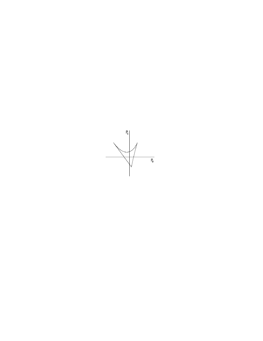
Figure 1: Orbit space III.2 and its section with a plane $p_{3}=\mbox{constant}$.

All $G$-invariant $C^{\infty}$ functions $f(x)$, defined on ${\mathchoice{\hbox{$\displaystyle\kern-0.56905pt1\kern-2.84526pt\mbox{\rm R}\kern-0.56905pt$}}{\hbox{$\textstyle\kern-0.56905pt1\kern-2.84526pt\mbox{\rm R}\kern-0.56905pt$}}{\hbox{$\scriptstyle\kern-0.56905pt1\kern-2.84526pt\mbox{\rm R}\kern-0.56905pt$}}{\hbox{$\scriptscriptstyle\kern-0.56905pt1\kern-2.84526pt\mbox{\rm R}\kern-0.56905pt$}}}^{n}$, can be expressed as $C^{\infty}$ functions of the basic invariants, so they define $C^{\infty}$ functions $\widehat{f}(p)$, defined on ${\mathchoice{\hbox{$\displaystyle\kern-0.56905pt1\kern-2.84526pt\mbox{\rm R}\kern-0.56905pt$}}{\hbox{$\textstyle\kern-0.56905pt1\kern-2.84526pt\mbox{\rm R}\kern-0.56905pt$}}{\hbox{$\scriptstyle\kern-0.56905pt1\kern-2.84526pt\mbox{\rm R}\kern-0.56905pt$}}{\hbox{$\scriptscriptstyle\kern-0.56905pt1\kern-2.84526pt\mbox{\rm R}\kern-0.56905pt$}}}^{q}$:

$$f(x)=\widehat{f}(p_{1}(x),\ldots,p_{q}(x))\to\widehat{f}(p_{1},\ldots,p_{q})$$

The functions $\widehat{f}(p)$ are defined also in points $p\notin{\cal S}$ but only the restriction $\widehat{f}(p)\mid_{p\in{\cal S}}$ has the same range as $f(x),\ x\in{\mathchoice{\hbox{$\displaystyle\kern-0.56905pt1\kern-2.84526pt\mbox{\rm R}\kern-0.56905pt$}}{\hbox{$\textstyle\kern-0.56905pt1\kern-2.84526pt\mbox{\rm R}\kern-0.56905pt$}}{\hbox{$\scriptstyle\kern-0.56905pt1\kern-2.84526pt\mbox{\rm R}\kern-0.56905pt$}}{\hbox{$\scriptscriptstyle\kern-0.56905pt1\kern-2.84526pt\mbox{\rm R}\kern-0.56905pt$}}}^{n}$, in fact $f(x)=f(p)$ if $p=p(x)$, that is if $p\in{\cal S}$.
All $G$-invariant $C^{\infty}$ functions can then be studied in the orbit space ${\cal S}$ but one needs to know exactly all equations and inequalities defining ${\cal S}$ and its strata.
A polynomial $f(p)$ is said $w$-homogeneous of weight $d$ if the polynomial $f(p(x))$ is homogeneous with degree $d$. Each coordinate $p_{1},\ldots,p_{q}$ of ${\mathchoice{\hbox{$\displaystyle\kern-0.56905pt1\kern-2.84526pt\mbox{\rm R}\kern-0.56905pt$}}{\hbox{$\textstyle\kern-0.56905pt1\kern-2.84526pt\mbox{\rm R}\kern-0.56905pt$}}{\hbox{$\scriptstyle\kern-0.56905pt1\kern-2.84526pt\mbox{\rm R}\kern-0.56905pt$}}{\hbox{$\scriptscriptstyle\kern-0.56905pt1\kern-2.84526pt\mbox{\rm R}\kern-0.56905pt$}}}^{q}$ has then a weight $d_{1},\ldots,d_{q}$.

The IBTs can be viewed as coordinate transformations of ${\mathchoice{\hbox{$\displaystyle\kern-0.56905pt1\kern-2.84526pt\mbox{\rm R}\kern-0.56905pt$}}{\hbox{$\textstyle\kern-0.56905pt1\kern-2.84526pt\mbox{\rm R}\kern-0.56905pt$}}{\hbox{$\scriptstyle\kern-0.56905pt1\kern-2.84526pt\mbox{\rm R}\kern-0.56905pt$}}{\hbox{$\scriptscriptstyle\kern-0.56905pt1\kern-2.84526pt\mbox{\rm R}\kern-0.56905pt$}}}^{q}$:

$$p_{i}^{\prime}=p_{i}^{\prime}(p_{1},\ldots,p_{q}),\qquad i=1,\ldots,q-1,\qquad p_{q}^{\prime}=p_{q}$$

The Jacobian matrix $J(p)$ inherits the properties of $J(x)$, in particular its matrix elements $J_{ij}(p)=\partial p_{i}^{\prime}(p)/\partial p_{j}$ are 0 or $w$-homogeneous polynomials in $p$ of weight $d_{i}-d_{j}$ and $\det J(p)$ is a non vanishing constant. The only coordinate transformations of ${\mathchoice{\hbox{$\displaystyle\kern-0.56905pt1\kern-2.84526pt\mbox{\rm R}\kern-0.56905pt$}}{\hbox{$\textstyle\kern-0.56905pt1\kern-2.84526pt\mbox{\rm R}\kern-0.56905pt$}}{\hbox{$\scriptstyle\kern-0.56905pt1\kern-2.84526pt\mbox{\rm R}\kern-0.56905pt$}}{\hbox{$\scriptscriptstyle\kern-0.56905pt1\kern-2.84526pt\mbox{\rm R}\kern-0.56905pt$}}}^{q}$ of interest are those corresponding to IBTs and they are called again IBTs (of ${\mathchoice{\hbox{$\displaystyle\kern-0.56905pt1\kern-2.84526pt\mbox{\rm R}\kern-0.56905pt$}}{\hbox{$\textstyle\kern-0.56905pt1\kern-2.84526pt\mbox{\rm R}\kern-0.56905pt$}}{\hbox{$\scriptstyle\kern-0.56905pt1\kern-2.84526pt\mbox{\rm R}\kern-0.56905pt$}}{\hbox{$\scriptscriptstyle\kern-0.56905pt1\kern-2.84526pt\mbox{\rm R}\kern-0.56905pt$}}}^{q}$).
The IBTs change the form of ${\cal S}$ but not its topological shape and stratification.

An IB is said regular if it does not exist any polynomial function $f(p)$ such that:

$$f(p_{1}(x),\ldots,p_{q}(x))=0\qquad\forall x\in{\mathchoice{\hbox{$\displaystyle\kern-0.56905pt1\kern-2.84526pt\mbox{\rm R}\kern-0.56905pt$}}{\hbox{$\textstyle\kern-0.56905pt1\kern-2.84526pt\mbox{\rm R}\kern-0.56905pt$}}{\hbox{$\scriptstyle\kern-0.56905pt1\kern-2.84526pt\mbox{\rm R}\kern-0.56905pt$}}{\hbox{$\scriptscriptstyle\kern-0.56905pt1\kern-2.84526pt\mbox{\rm R}\kern-0.56905pt$}}}^{n}$$

Otherwise the IB is said non regular. Obviously $f(p)$ cannot be solved with respect of any of the variables, otherwise the basis would not be minimal.
A linear group $G$ with a regular $IB$ is said coregular. Otherwise it is said non-coregular.
If the basis is non regular then generally it exists an ideal of polynomial relations between the elements of the IB and the (independent) generators of this ideal $f_{1},\ldots,f_{r}$ can always be chosen homogeneous. The orbit space ${\cal S}$ must then be contained in the surface ${\cal Z}$ of ${\mathchoice{\hbox{$\displaystyle\kern-0.56905pt1\kern-2.84526pt\mbox{\rm R}\kern-0.56905pt$}}{\hbox{$\textstyle\kern-0.56905pt1\kern-2.84526pt\mbox{\rm R}\kern-0.56905pt$}}{\hbox{$\scriptstyle\kern-0.56905pt1\kern-2.84526pt\mbox{\rm R}\kern-0.56905pt$}}{\hbox{$\scriptscriptstyle\kern-0.56905pt1\kern-2.84526pt\mbox{\rm R}\kern-0.56905pt$}}}^{q}$ defined by the equations:

$$f_{1}(p)=0,\ldots,\quad f_{r}(p)=0$$

and has the same dimension $q-r$ of ${\cal Z}$. ${\cal Z}$ is called the surface of the relations and the couple $(q,q-r)$ the regularity type (or $r$-type) of the IB and of the group $G$.
When $G$ is coregular there are no relations, $r=0$, and ${\cal Z}\equiv{\mathchoice{\hbox{$\displaystyle\kern-0.56905pt1\kern-2.84526pt\mbox{\rm R}\kern-0.56905pt$}}{\hbox{$\textstyle\kern-0.56905pt1\kern-2.84526pt\mbox{\rm R}\kern-0.56905pt$}}{\hbox{$\scriptstyle\kern-0.56905pt1\kern-2.84526pt\mbox{\rm R}\kern-0.56905pt$}}{\hbox{$\scriptscriptstyle\kern-0.56905pt1\kern-2.84526pt\mbox{\rm R}\kern-0.56905pt$}}}^{q}$, so ${\cal S}$ is $q$-dimensional.

In a point $x\in\Sigma\subset{\mathchoice{\hbox{$\displaystyle\kern-0.56905pt1\kern-2.84526pt\mbox{\rm R}\kern-0.56905pt$}}{\hbox{$\textstyle\kern-0.56905pt1\kern-2.84526pt\mbox{\rm R}\kern-0.56905pt$}}{\hbox{$\scriptstyle\kern-0.56905pt1\kern-2.84526pt\mbox{\rm R}\kern-0.56905pt$}}{\hbox{$\scriptscriptstyle\kern-0.56905pt1\kern-2.84526pt\mbox{\rm R}\kern-0.56905pt$}}}^{n}$, the number of linear independent gradients of the basic invariants is equal to the dimension of the stratum $p(\Sigma)\subset{\cal S}$. It is convenient to construct the $q\times q$ Grammian matrix $P(x)$ with elements $P_{ab}(x)$ that are scalar products between the gradients of the basic invariants:

$$P_{ab}(x)=(\nabla p_{a}(x),\nabla p_{b}(x))$$

$P(x)$ is then positive semidefinite $\forall x\in{\mathchoice{\hbox{$\displaystyle\kern-0.56905pt1\kern-2.84526pt\mbox{\rm R}\kern-0.56905pt$}}{\hbox{$\textstyle\kern-0.56905pt1\kern-2.84526pt\mbox{\rm R}\kern-0.56905pt$}}{\hbox{$\scriptstyle\kern-0.56905pt1\kern-2.84526pt\mbox{\rm R}\kern-0.56905pt$}}{\hbox{$\scriptscriptstyle\kern-0.56905pt1\kern-2.84526pt\mbox{\rm R}\kern-0.56905pt$}}}^{n}$, and for $x\in\Sigma\subset{\mathchoice{\hbox{$\displaystyle\kern-0.56905pt1\kern-2.84526pt\mbox{\rm R}\kern-0.56905pt$}}{\hbox{$\textstyle\kern-0.56905pt1\kern-2.84526pt\mbox{\rm R}\kern-0.56905pt$}}{\hbox{$\scriptstyle\kern-0.56905pt1\kern-2.84526pt\mbox{\rm R}\kern-0.56905pt$}}{\hbox{$\scriptscriptstyle\kern-0.56905pt1\kern-2.84526pt\mbox{\rm R}\kern-0.56905pt$}}}^{n}$ $\mbox{rank}P(x)$ equals the dimension of the stratum $p(\Sigma)$ of ${\cal S}$.
Because of the covariance of the gradients of $G$-invariant functions ($\nabla f(g\cdot x)=g\cdot\nabla f(x)$) and of the orthogonality of $G$ (which implies the invariance of the scalar products), the matrix elements $P_{ab}(x)$ are $G$-invariant homogeneous polynomial functions of degree $d_{a}+d_{b}-2$. Then, all the matrix elements of $P(x)$ can be expressed as polynomials of the basic invariants. One can then define a matrix $\widehat{P}(p)$ in ${\mathchoice{\hbox{$\displaystyle\kern-0.56905pt1\kern-2.84526pt\mbox{\rm R}\kern-0.56905pt$}}{\hbox{$\textstyle\kern-0.56905pt1\kern-2.84526pt\mbox{\rm R}\kern-0.56905pt$}}{\hbox{$\scriptstyle\kern-0.56905pt1\kern-2.84526pt\mbox{\rm R}\kern-0.56905pt$}}{\hbox{$\scriptscriptstyle\kern-0.56905pt1\kern-2.84526pt\mbox{\rm R}\kern-0.56905pt$}}}^{q}$ such that:

$$P_{ab}(x)=\widehat{P}_{ab}(p_{1}(x),\ldots,p_{q}(x))=\widehat{P}_{ab}(p)\quad\forall x\in{\mathchoice{\hbox{$\displaystyle\kern-0.56905pt1\kern-2.84526pt\mbox{\rm R}\kern-0.56905pt$}}{\hbox{$\textstyle\kern-0.56905pt1\kern-2.84526pt\mbox{\rm R}\kern-0.56905pt$}}{\hbox{$\scriptstyle\kern-0.56905pt1\kern-2.84526pt\mbox{\rm R}\kern-0.56905pt$}}{\hbox{$\scriptscriptstyle\kern-0.56905pt1\kern-2.84526pt\mbox{\rm R}\kern-0.56905pt$}}}^{n}\ \mbox{and}\ p=p(x)$$

At the point $p=p(x)$, image in ${\mathchoice{\hbox{$\displaystyle\kern-0.56905pt1\kern-2.84526pt\mbox{\rm R}\kern-0.56905pt$}}{\hbox{$\textstyle\kern-0.56905pt1\kern-2.84526pt\mbox{\rm R}\kern-0.56905pt$}}{\hbox{$\scriptstyle\kern-0.56905pt1\kern-2.84526pt\mbox{\rm R}\kern-0.56905pt$}}{\hbox{$\scriptscriptstyle\kern-0.56905pt1\kern-2.84526pt\mbox{\rm R}\kern-0.56905pt$}}}^{q}$ of the point $x\in{\mathchoice{\hbox{$\displaystyle\kern-0.56905pt1\kern-2.84526pt\mbox{\rm R}\kern-0.56905pt$}}{\hbox{$\textstyle\kern-0.56905pt1\kern-2.84526pt\mbox{\rm R}\kern-0.56905pt$}}{\hbox{$\scriptstyle\kern-0.56905pt1\kern-2.84526pt\mbox{\rm R}\kern-0.56905pt$}}{\hbox{$\scriptscriptstyle\kern-0.56905pt1\kern-2.84526pt\mbox{\rm R}\kern-0.56905pt$}}}^{n}$ through the orbit map, the matrix $\widehat{P}(p)$ is the same as the matrix $P(x)$. The matrix $\widehat{P}(p)$ is however defined in all ${\mathchoice{\hbox{$\displaystyle\kern-0.56905pt1\kern-2.84526pt\mbox{\rm R}\kern-0.56905pt$}}{\hbox{$\textstyle\kern-0.56905pt1\kern-2.84526pt\mbox{\rm R}\kern-0.56905pt$}}{\hbox{$\scriptstyle\kern-0.56905pt1\kern-2.84526pt\mbox{\rm R}\kern-0.56905pt$}}{\hbox{$\scriptscriptstyle\kern-0.56905pt1\kern-2.84526pt\mbox{\rm R}\kern-0.56905pt$}}}^{q}$, also outside ${\cal S}$, but only in ${\cal S}$ it reproduces $P(x),\ \forall x\in{\mathchoice{\hbox{$\displaystyle\kern-0.56905pt1\kern-2.84526pt\mbox{\rm R}\kern-0.56905pt$}}{\hbox{$\textstyle\kern-0.56905pt1\kern-2.84526pt\mbox{\rm R}\kern-0.56905pt$}}{\hbox{$\scriptstyle\kern-0.56905pt1\kern-2.84526pt\mbox{\rm R}\kern-0.56905pt$}}{\hbox{$\scriptscriptstyle\kern-0.56905pt1\kern-2.84526pt\mbox{\rm R}\kern-0.56905pt$}}}^{n}$.
The properties of the matrix $\widehat{P}(p)$ depend on the definition of $P(x)$ and are the following:

1. $\widehat{P}(p)$ is a real, symmetric $q\times q$ matrix.

2. $\widehat{P}(p)$ is positive semidefinite in ${\cal S}$. ${\cal S}$ is the only region of ${\cal Z}$ where $\widehat{P}(p)\geq 0$.

3. $\mbox{rank}\widehat{P}(p)$ equals the dimension of the stratum containing $p$.

4. the matrix elements $\widehat{P}_{ab}(p)$ are $w$-homogeneous polynomial functions of weight $d_{a}+d_{b}-2$ and the last row and column of $\widehat{P}(p)$ have the fixed form:

   $$\widehat{P}_{qa}(p)=\widehat{P}_{aq}(p)=2d_{a}p_{a}\qquad\forall a=1,\ldots,q$$

5. $\widehat{P}(p)$ transforms as a contravariant tensor under IBTs:

   $$P_{ab}^{\prime}(p^{\prime})=J_{ai}(p)J_{bj}(p)P_{ij}(p)$$

The matrix $\widehat{P}(p)$ completely determines ${\cal S}$ and its stratification. Defining ${\cal S}_{k}$ the union of all $k$-dimensional strata of ${\cal S}$, one has:

$${\cal S}=\{p\in{\cal Z}\mid\widehat{P}(p)\geq 0\}$$

$${\cal S}_{k}=\{p\in{\cal Z}\mid\widehat{P}(p)\geq 0,\ \mbox{rank}P(p)=k\}$$

The principal stratum has dimension $q-r$, equal to the maximum rank of $\widehat{P}(p)$, with $r$ the number of independent relations among the $p_{i}(x)$, and coincides with ${\cal S}_{q-r}$. (Obviously if $G$ is coregular $r=0$ and ${\cal Z}\equiv{\mathchoice{\hbox{$\displaystyle\kern-0.56905pt1\kern-2.84526pt\mbox{\rm R}\kern-0.56905pt$}}{\hbox{$\textstyle\kern-0.56905pt1\kern-2.84526pt\mbox{\rm R}\kern-0.56905pt$}}{\hbox{$\scriptstyle\kern-0.56905pt1\kern-2.84526pt\mbox{\rm R}\kern-0.56905pt$}}{\hbox{$\scriptscriptstyle\kern-0.56905pt1\kern-2.84526pt\mbox{\rm R}\kern-0.56905pt$}}}^{q}$).
To find out ${\cal S}_{k}$ one may impose that all the principal minors of $\widehat{P}(p)$ of order greater than $k$ have zero determinant and that at least one of of those of order $k$ have non zero determinant. From this one sees that ${\cal S}$ is semialgebraic because it is defined through algebraic equations and inequalities.
In order to classify orbit spaces, it is sufficient to classify the corresponding matrices $\widehat{P}(p)$, as they determine ${\cal S}$ completely and this has been done in [1, 4].

3 Determination of the Allowable $\widehat{P}$-matrices of Compact Linear Groups through the Canonical Equation

The polynomials defining the singular strata of ${\cal S}$ (and also the principal stratum if $G$ is non-coregular) must satisfy a differential relation (that characterize them) that has been crucial in [1, 4, 3] to determine the $\widehat{P}$-matrices without the explicit use of the IB’s. Let’s see the origin of this relation.
Let $\sigma$ be a primary stratum of ${\cal S}$ and $I(\sigma)$ the ideal of the polynomials defined in ${\mathchoice{\hbox{$\displaystyle\kern-0.56905pt1\kern-2.84526pt\mbox{\rm R}\kern-0.56905pt$}}{\hbox{$\textstyle\kern-0.56905pt1\kern-2.84526pt\mbox{\rm R}\kern-0.56905pt$}}{\hbox{$\scriptstyle\kern-0.56905pt1\kern-2.84526pt\mbox{\rm R}\kern-0.56905pt$}}{\hbox{$\scriptscriptstyle\kern-0.56905pt1\kern-2.84526pt\mbox{\rm R}\kern-0.56905pt$}}}^{q}$ vanishing in $\sigma$. Then $\Sigma=\{x\in{\mathchoice{\hbox{$\displaystyle\kern-0.56905pt1\kern-2.84526pt\mbox{\rm R}\kern-0.56905pt$}}{\hbox{$\textstyle\kern-0.56905pt1\kern-2.84526pt\mbox{\rm R}\kern-0.56905pt$}}{\hbox{$\scriptstyle\kern-0.56905pt1\kern-2.84526pt\mbox{\rm R}\kern-0.56905pt$}}{\hbox{$\scriptscriptstyle\kern-0.56905pt1\kern-2.84526pt\mbox{\rm R}\kern-0.56905pt$}}}^{n}\mid p(x)\in\sigma\}$ is a connected component of a stratum of ${\mathchoice{\hbox{$\displaystyle\kern-0.56905pt1\kern-2.84526pt\mbox{\rm R}\kern-0.56905pt$}}{\hbox{$\textstyle\kern-0.56905pt1\kern-2.84526pt\mbox{\rm R}\kern-0.56905pt$}}{\hbox{$\scriptstyle\kern-0.56905pt1\kern-2.84526pt\mbox{\rm R}\kern-0.56905pt$}}{\hbox{$\scriptscriptstyle\kern-0.56905pt1\kern-2.84526pt\mbox{\rm R}\kern-0.56905pt$}}}^{n}$. For all $\widehat{f}\in I(\sigma)$, $f(x)=\widehat{f}(p(x))$ is a $G$-invariant function that vanishes on $\Sigma$. Then in all regular points $x$ of $\Sigma$ one must have that $\ \nabla f(x)|_{x\in\Sigma}\;\perp\;\Sigma\$ because $f(x)$ is constant in $\Sigma$, and that $\ \nabla f(x)|_{x\in\Sigma}\$ is tangent to $\Sigma$ because $f(x)$ is $G$-invariant and the gradients of $G$-invariant functions are tangent to the strata. Then the only possibility is that:

$$\nabla f(x)|_{x\in\Sigma}\ =\ 0$$

Applying the partial differentiation rule and taking the scalar product with $\nabla p_{a}(x)$, $a=1,\ldots,q$, one obtains $q$ relations expressed only in terms of the $p_{i}(x)$, that can so be defined also in ${\mathchoice{\hbox{$\displaystyle\kern-0.56905pt1\kern-2.84526pt\mbox{\rm R}\kern-0.56905pt$}}{\hbox{$\textstyle\kern-0.56905pt1\kern-2.84526pt\mbox{\rm R}\kern-0.56905pt$}}{\hbox{$\scriptstyle\kern-0.56905pt1\kern-2.84526pt\mbox{\rm R}\kern-0.56905pt$}}{\hbox{$\scriptscriptstyle\kern-0.56905pt1\kern-2.84526pt\mbox{\rm R}\kern-0.56905pt$}}}^{q}$:

$$0=\nabla f(x)|_{x\in\Sigma}=\sum_{b=1}^{q}\nabla p_{b}(x)\left.\frac{\partial f(x)}{\partial p_{b}(x)}\right|_{x\in\Sigma}=\sum_{b=1}^{q}(\nabla p_{a}(x),\nabla p_{b}(x))\left.\frac{\partial f(x)}{\partial p_{b}(x)}\right|_{x\in\Sigma}=$$

$$=\sum_{b=1}^{q}{\widehat{P}}_{ab}(p(x))\left.\frac{\partial f(p(x))}{\partial p_{b}(x)}\right|_{x\in\Sigma}=\sum_{b=1}^{q}{\widehat{P}}_{ab}(p)\left.\frac{\partial f(p)}{\partial p_{b}}\right|_{p\in\sigma},\qquad a=1,\ldots,q$$

This means that:

$$\left.\sum_{b=1}^{q}{\widehat{P}}_{ab}(p)\partial_{b}f(p)\right|_{p\in\sigma}\in I(\sigma),\qquad a=1,\ldots,q$$

where $\partial_{b}$ means partial derivation with respect to $p_{b}$.
It is convenient to distinguish two cases:

1. $I(\sigma)$ has only one generator $a(p)$. In this case one obtains the following relations:

   $$\sum_{b=1}^{q}{\widehat{P}}_{ab}(p)\partial_{b}a(p)=\lambda_{a}(p)a(p)\qquad a=1,\ldots,q$$

   with the $\lambda_{a}(p)$ $w$-homogeneous polynomials of weight $d_{a}-2$. In this case $\sigma$ is a surface of dimension $q-1$ and its intersection with the region $\widehat{P}(p)\geq 0$ gives a singular strata of maximal dimension if $G$ is coregular or the principal stratum if $G$ is non-coregular of $r$-type $(q,q-1)$. In this last case the equation $a(p)=0$ defines ${\cal Z}$.

2. $I(\sigma)$ has more independent generators $a^{(1)}(p),\ldots,a^{(s)}(p)$. In this case one obtains the following relations:

   $$\sum_{b=1}^{q}{\widehat{P}}_{ab}(p)\partial_{b}a^{(j)}(p)=\sum_{i=1}^{s}\lambda_{a}^{(i,j)}(p)a^{(i)}(p)\qquad a=1,\ldots,q,\ j=1,\ldots,s$$

   with the $\lambda_{a}^{(i,j)}(p)$ $w$-homogeneous polynomials of weight $d_{a}-2+w(a^{(j)})-w(a^{(i)})$. $\sigma$ in this case is a surface of dimension $q-s$. It can be a principal stratum only if $G$ is non-coregular of $r$-type $(q,q-s)$. In all other cases it is a singular stratum.

Both the two relations written are called master relations. At the moment only the case of $(q-1)$-dimensional strata has been investigated: the coregular case is presented in [1] and the non-coregular case of $r$-type $(q,q-1)$ in [3] and all what follows concerns only $(q-1)$-dimensional strata.

It has been proved in [1] that all irreducible polynomials $a(p)$ that satisfy the master relation must be factors of $\det{\widehat{P}}(p)$. Any product of them satisfies the master relation too. All these polynomials are called active. The product $A(p)$ of all irreducible active polynomials is called the complete (active) factor of $\det{\widehat{P}}(p)$. The surface $\sigma=\{p\in{\cal Z}\mid\widehat{P}(p)\geq 0,A(p)=0\}$ coincides with the whole boundary of ${\cal S}$ if $G$ is coregular (${\cal Z}\equiv{\mathchoice{\hbox{$\displaystyle\kern-0.56905pt1\kern-2.84526pt\mbox{\rm R}\kern-0.56905pt$}}{\hbox{$\textstyle\kern-0.56905pt1\kern-2.84526pt\mbox{\rm R}\kern-0.56905pt$}}{\hbox{$\scriptstyle\kern-0.56905pt1\kern-2.84526pt\mbox{\rm R}\kern-0.56905pt$}}{\hbox{$\scriptscriptstyle\kern-0.56905pt1\kern-2.84526pt\mbox{\rm R}\kern-0.56905pt$}}}^{n}$ in this case) or coincides with the whole principal stratum of ${\cal S}$ if $G$ is non-coregular of $r$-type $(q,q-1)$. $\det{\widehat{P}}(p)$ may contain a non active factor $B(p)$ that is called passive. $A(p)$ and $B(p)$ are uniquely defined except by non-zero constant factors.
In [1] are studied the properties of the master relation with respect to IBTs, and the main results are the following:

1. In some IB, called $A$-bases, the master relation has the following canonical form:

   $$\sum_{b=1}^{q}\widehat{P}_{ab}(p)\partial_{b}A(p)=2w(A)\delta_{aq}A(p)\qquad a=1,\ldots,q$$

   The case $a=q$ is just a homogeneity condition on $A(p)$ and only the cases $a=1,\ldots,q-1$ are characteristic of the $(q-1)$-dimensional strata. The variable $p_{q}$ can then be easily eliminated from the equation if one restricts to a plane $\Pi$ of constant $p_{q}$, for example $\Pi=\{p\in{\mathchoice{\hbox{$\displaystyle\kern-0.56905pt1\kern-2.84526pt\mbox{\rm R}\kern-0.56905pt$}}{\hbox{$\textstyle\kern-0.56905pt1\kern-2.84526pt\mbox{\rm R}\kern-0.56905pt$}}{\hbox{$\scriptstyle\kern-0.56905pt1\kern-2.84526pt\mbox{\rm R}\kern-0.56905pt$}}{\hbox{$\scriptscriptstyle\kern-0.56905pt1\kern-2.84526pt\mbox{\rm R}\kern-0.56905pt$}}}^{q}\mid p_{q}=1\}$.

2. In all $A$-bases, the restriction $A(p)\mid_{p\in\Pi}$, has at most one local non-degenerate extremum in $\Pi$, outside of the region $A(p)\mid_{p\in\Pi}\;=0$, at the point $p_{0}=(0,\ldots,0,1)$.

If $G$ is coregular one has also the following results:

1. $p_{0}$ always exists and lies in the interior of ${\cal S}$.

2. In some $A$-bases, the standard $A$-bases, $\widehat{P}(p)$ evaluated at $p_{0}$ is diagonal.

Properties 3. and 4. exclude linear terms in $A(p)\mid_{p\in\Pi}$ and requires that all the quadratic terms $p_{i}^{2}$ have coefficients of equal sign (negative if one requires $A(p)\mid_{p\in\Pi}$ to be maximum at $p_{0}$) and that there are no mixed quadratic terms $p_{i}p_{j}$. The weight $w(A)$ of $A(p)$ is then bounded: $2d_{1}\leq w(A)\leq w(\det\widehat{P})=2\sum_{i=1}^{q}(d_{i}-1)$.
If $G$ is non-coregular properties 3. and 4. are not valid but $A(p)$ must satisfy in addition a second order boundary condition [3].

Given the IB, and following the lines reported above, it is easy to determine the matrix $\widehat{P}(p)$, the complete factor $A(p)$, and the subset ${\cal S}$ of ${\mathchoice{\hbox{$\displaystyle\kern-0.56905pt1\kern-2.84526pt\mbox{\rm R}\kern-0.56905pt$}}{\hbox{$\textstyle\kern-0.56905pt1\kern-2.84526pt\mbox{\rm R}\kern-0.56905pt$}}{\hbox{$\scriptstyle\kern-0.56905pt1\kern-2.84526pt\mbox{\rm R}\kern-0.56905pt$}}{\hbox{$\scriptscriptstyle\kern-0.56905pt1\kern-2.84526pt\mbox{\rm R}\kern-0.56905pt$}}}^{q}$ that represents the orbit space of the group action. The $\widehat{P}$-matrices can however be calculated and classified without the knowledge of the IB’s. The many conditions found on the form of a general $\widehat{P}$-matrix and on the complete factor $A$ allow to find out all possible solutions to the canonical equation that are compatible with these conditions (the master relation in its canonical form is used now to find out the $\widehat{P}$-matrices, so it is better to call it equation instead of relation).

In [1, 4] the canonical equation is solved for the case of coregular groups. We only fixed the number $q$ of the basic invariants and we considered all matrix elements $\widehat{P}_{ab}(p)$ and $A(p)$ and $B(p)$ as unknown $w$-homogeneous polynomials satisfying the following initial conditions:

1. $\widehat{P}(p)$ is a real, symmetric $q\times q$ matrix;

2. the matrix elements $\widehat{P}_{ab}(p)$ are $w$-homogeneous polynomial functions of weight $d_{a}+d_{b}-2$ and the last row and column of $\widehat{P}(p)$ have the fixed form:

   $$\widehat{P}_{qa}(p)=\widehat{P}_{aq}(p)=2d_{a}p_{a}\qquad\forall a=1,\ldots,q$$

3. $\widehat{P}(p_{0})$ is diagonal and positive definite;

4. $A(p)$ is $w$-homogeneous of weight $w(A)$ such that: $2d_{1}\leq w(A)\leq w(\det{\widehat{P}})$. Its restriction to the plane $p_{q}=1$ has no linear terms and only quadratic terms of the type $-k_{i}p_{i}^{2}$ with $k_{i}>0$.

5. $A(p)$ is a factor of $\det{\widehat{P}}$, so the equation $A(p)B(p)=\det{\widehat{P}}(p)$ defines $B(p)$.

6. the canonical equation must be satisfied.

In all these unknown polynomials the dependence on the variable $p_{1}$ can always be rendered explicit even if all degrees $d_{i},\ i\neq q$ are unknown. Items 5. and 6. give a system of coupled differential equations that should be solved by unknown $w$-homogeneous polynomial functions. The initial conditions imposed were so strong that this system could be solved analytically and it gave only a finite number of different solutions for each value of the dimension $q$ ($q$ = 2, 3, 4, but there is no reason to believe that this will not be true for higher values of $q$). The matrices $\widehat{P}(p)$ that together with the corresponding complete factor $A(p)$ satisfy these initial conditions, are such that $\widehat{P}(p)\geq 0$ only in a connected subset ${\cal S}$ of ${\mathchoice{\hbox{$\displaystyle\kern-0.56905pt1\kern-2.84526pt\mbox{\rm R}\kern-0.56905pt$}}{\hbox{$\textstyle\kern-0.56905pt1\kern-2.84526pt\mbox{\rm R}\kern-0.56905pt$}}{\hbox{$\scriptstyle\kern-0.56905pt1\kern-2.84526pt\mbox{\rm R}\kern-0.56905pt$}}{\hbox{$\scriptscriptstyle\kern-0.56905pt1\kern-2.84526pt\mbox{\rm R}\kern-0.56905pt$}}}^{q}$ (whose boundary satisfy the equation $A(p)=0$) and are called allowable $\widehat{P}$-matrices. The name originates from the fact that they are potentially determined by an IB of an existing group $G$, but it is not known in general if that group does really exist. It is clear however that all $\widehat{P}$- matrices determined by the IB of the existing compact coregular groups are allowable $\widehat{P}$-matrices.

This approach has been recently applied with success to the determination of the allowable $\widehat{P}$-matrices associated to compact non-coregular linear groups of $r$-type $(q,q-1)$ [3]. The initial conditions 3. and 4. for the case of coregular groups are no longer valid and must be replaced by the following two conditions:

1. $A(p)$ is $w$-homogeneous of weight $w(A)\leq w(\det\widehat{P})$.

2. $A(p)$ satisfies the second order boundary condition [3].

Then one proceeds as in the coregular case. Here not all solutions found are such that $\widehat{P}(p)\geq 0$ in a connected subset of ${\mathchoice{\hbox{$\displaystyle\kern-0.56905pt1\kern-2.84526pt\mbox{\rm R}\kern-0.56905pt$}}{\hbox{$\textstyle\kern-0.56905pt1\kern-2.84526pt\mbox{\rm R}\kern-0.56905pt$}}{\hbox{$\scriptstyle\kern-0.56905pt1\kern-2.84526pt\mbox{\rm R}\kern-0.56905pt$}}{\hbox{$\scriptscriptstyle\kern-0.56905pt1\kern-2.84526pt\mbox{\rm R}\kern-0.56905pt$}}}^{q}$, so, a posteriori, one has to discard some solutions. It can however be proved that when the point $p_{0}$, where $A(p)\mid_{p\in\Pi}$ has an extremum, exists and does not belong to ${\cal Z}$, then the allowable $\widehat{P}$-matrices of the non-coregular groups of $r$-type $(q,q-1)$ are necessarily allowable $\widehat{P}$-matrices of coregular groups with $q$ basic invariants. In this case the orbit spaces ${\cal S}^{\prime}$ of the non-coregular groups lie always in some connected $(q-1)$-dimensional singular stratum of the orbit space ${\cal S}$ of a coregular group.

In table 1 I report all 2-, 3- and 4-dimensional allowable $\widehat{P}$-matrices for coregular groups, showing the corresponding weights $[d_{1},\ldots,d_{q-1},2]$ of the $p_{i}$ and the weight $w(A)$ of the complete factor $A(p)$. The parameters $j_{i}$ and $s$ that appear in the table are arbitrary positive integers limited only by $d_{1}\geq\cdots\geq d_{q-1}\geq 2$.
The explicit forms of these allowable $\widehat{P}$-matrices are given in [1, 4].
These allowable $\widehat{P}$-matrices share the following properties:

1. For each number $q$, there are a finite number of classes of allowable $q\times q$ $\widehat{P}$-matrices. In each class the $\widehat{P}$-matrices differ only in some positive integer parameters $j_{i}$ and in a scale factor $s$. These parameters fix also the values of the degrees $[d_{1},d_{2},\ldots,d_{q}-1]$. In $\Pi=\{p\in{\mathchoice{\hbox{$\displaystyle\kern-0.56905pt1\kern-2.84526pt\mbox{\rm R}\kern-0.56905pt$}}{\hbox{$\textstyle\kern-0.56905pt1\kern-2.84526pt\mbox{\rm R}\kern-0.56905pt$}}{\hbox{$\scriptstyle\kern-0.56905pt1\kern-2.84526pt\mbox{\rm R}\kern-0.56905pt$}}{\hbox{$\scriptscriptstyle\kern-0.56905pt1\kern-2.84526pt\mbox{\rm R}\kern-0.56905pt$}}}^{q}|p_{q}=1\}$ all the matrices that differ only for the value of $s$ become identical.

2. In convenient $A$-bases all coefficients of the $\widehat{P}$-matrix elements are integer numbers.

In [4, 5] the classes $A9(j_{1})$ and $A10(j_{1})$ were forgotten. These classes of solutions have been determined by applying the induction rules [6] to the case $q=3$. These induction rules permit to write down easily most of the solutions for the $(q+1)$-dimensional coregular case once one knows those of the $q$-dimensional case. The 4 induction rules discovered up to now when applied to the solutions corresponding to $q=2,3$ give all solutions of the case $q=3,4$, except when the complete factor contain a term in $p_{1}^{q}$ (and this seems the case of all irreducible finite groups generated by reflections) and except the class $D2$ (that probably can be derived from the class III.3 with an induction rule not yet discovered). The induction rules probably reflect some properties of groups but they are not yet understood.

In [3] are determined all allowable $\widehat{P}$-matrices for non-coregular groups of $r$-type $(q,q-1)$, tht is groups with 3 invariants among which there is one algebraic relation. It results only one class of allowable $\widehat{P}$-matrices for these groups and these $\widehat{P}$-matrices are the same as those for the coregular case with 3 invariants classified in [1] as $I(1,1)$. The only difference is that the principal stratum now is the 2-dimensional surface that makes up the boundary of ${\cal S}$ in the coregular case. It is possible that all orbit spaces of non-coregular groups of $r$-type $(q,q-1)$ occour at the border of the orbit spaces of coregular groups.

Table 1: ALLOWABLE $\widehat{P}$- MATRICES OF COREGULAR GROUPS OF DIMENSION $q=2,3,4$.

$q$	CLASS	$w(A)$	$[d_{1},\ldots,d_{q}]$
2	$I_{2}$	$2d_{1}$	$[s,2]$
3	$I(j_{1},j_{2})$	$2d_{1}$	$[s(j_{1}+j_{2})/2,s,2]$
	$II(j_{1})$	$2d_{1}+d_{2}$	$[s(j_{1}+1),2s,2]$
	$III.1$	$3d_{1}$	$[4s,3s,2]$
	$III.2$	$3d_{1}$	$[6s,4s,2]$
	$III.3$	$3d_{1}$	$[10s,6s,2]$
4	$A1(j_{1},j_{2},j_{3},j_{4})$	$2d_{1}$	$[s(j_{1}+j_{2})(j_{3}+j_{4})/4,s(j_{1}+j_{2})/2,s,2]$
	$A3(j_{1},j_{2},j_{3})$	$2d_{1}+d_{3}$	$[s(j_{1}+1)(j_{2}+j_{3})/2,s(j_{1}+1),2s,2]$
	$A2(j_{1},j_{2},j_{3},j_{4})$	$2d_{1}$	$[s((j_{1}+1)(j_{2}+j_{3})/2+j_{4}),s(j_{1}+1),2s,2]$
	$A4(j_{1},j_{2})$	$2d_{1}+j_{1}d_{3}$	$2sj_{2},s(j_{1}+j_{2}),2s,2]$
	$A5(j_{1},j_{2},j_{3})$	$2d_{1}+d_{2}$	$[s(j_{1}(j_{2}+1)+j_{3}),2s(j_{2}+1),2s,2]$
	$A6(j_{1},j_{2},j_{3})$	$2d_{1}+d_{2}$	$[s(j_{1}+j_{2})(j_{3}+1)/2,s(j_{1}+j_{2}),s,2]$
	$A7(j_{1},j_{2})$	$2d_{1}+d_{2}+d_{3}$	$[sj_{1}(j_{2}+1),2sj_{1},2s,2]$
	$A8(j_{1},j_{2})$	$2d_{1}+2d_{2}$	$[s(j_{1}+1),s(j_{2}+1),2s,2]$
	$A9(j_{1})$	$2d_{1}+d_{3}$	$[2s(j_{1}+1),s(j_{1}+1),2s,2]$
	$A10(j_{1})$	$2d_{1}+d_{2}$	$[s(j_{1}+1),2s,s,2]$
	$B1(j_{1})$	$2d_{1}$	$[6sj_{1},4s,3s,2]$
	$B2$	$3d_{1}$	$[4s,3s,3s,2]$
	$B3(j_{1},j_{2})$	$3d_{1}$	$[2s(j_{1}+j_{2}),3s(j_{1}+j_{2})/2,s,2]$
	$B4(j_{1})$	$3d_{1}+d_{3}$	$[4sj_{1},3sj_{1},2s,2]$
	$C1(j_{1},j_{2})$	$2d_{1}$	$[3s(j_{1}+2j_{2}),6s,4s,2]$
	$C2(j_{1})$	$2d_{1}+d_{2}$	$[6sj_{1},6s,4s,2]$
	$C3(j_{1})$	$2d_{1}+2d_{2}$	$[3s(j_{1}+1),6s,4s,2]$
	$C4$	$3d_{1}$	$[6s,4s,3s,2]$
	$C5(j_{1},j_{2})$	$3d_{1}$	$[3s(j_{1}+j_{2}),2s(j_{1}+j_{2}),s,2]$
	$C6(j_{1})$	$3d_{1}+d_{3}$	$[6sj_{1},4sj_{1},2s,2]$
	$D1(j_{1})$	$2d_{1}$	$[15sj_{1},10s,6s,2]$
	$D2$	$3d_{1}$	$[10s,6s,4s,2]$
	$D3(j_{1},j_{2})$	$3d_{1}$	$[5s(j_{1}+j_{2}),3s(j_{1}+j_{2}),s,2]$
	$D4(j_{1})$	$3d_{1}+d_{3}$	$[10sj_{1},6sj_{1},2s,2]$
	$E1$	$4d_{1}$	$[5s,4s,3s,2]$
	$E2$	$4d_{1}$	$[6s,4s,4s,2]$
	$E3$	$4d_{1}$	$[8s,6s,4s,2]$
	$E4$	$4d_{1}$	$[12s,8s,6s,2]$
	$E5$	$4d_{1}$	$[30s,20s,12s,2]$

Notation. $q$: number of basic invariants and dimension of the $\widehat{P}$-matrices. CLASS: class of $\widehat{P}$-matrices in the notation of [1, 4]. $w(A)$ degree of the active factor $A(p)$ determining the boundary of the orbit space. $[d_{1},\ldots,d_{q}]$: degree of the basic invariants.

4 Orbit Spaces of Coregular Compact Groups

All linear compact groups generate a $\widehat{P}$-matrix that must be an allowable $\widehat{P}$-matrix. The converse may also be true but one must find the linear groups corresponding to a given allowable $\widehat{P}$-matrix.

In the case of irreducible finite groups generated by reflections the IB are well known and when these IB contain 2, 3 and 4 basic invariants the corresponding $\widehat{P}$-matrices have been determined [7]. All these $\widehat{P}$-matrices, after a proper IBT, exactly coincide with those in the classification of allowable $\widehat{P}$-matrices reported in [1, 4].

In the case of compact Lie groups the IB is known only in few cases. G. W. Schwarz [8] gave a classification of all complex coregular representations of complex simple Lie groups, together with the number and degrees of the basic invariants, and for some groups also some hints to write down the integrity basis.
From this classification it is possible to deduce all real coregular representations of compact simple Lie groups. Here under I shall sketch how this has been possible. Proofs and details can be found in [9, 10].

• Let $G$ be a compact Lie group and $G_{c}$ be its complexification. $G_{c}$ is the smallest complex Lie group that contains $G$ and $G$ is a maximal compact subgroup of $G_{c}$.

• Let $\varphi$ be a real representation of $G$ in a real vector space $W_{\varphi}$. $\varphi$ defines uniquely a complex representation of $G_{c}$ in the complex space $V_{\varphi}={\mathchoice{\hbox{$\displaystyle\kern-0.56905pt{\rm C}\kern-4.2679pt\raise 0.56905pt\hbox{\vrule height=6.0pt}\kern 3.69885pt$}}{\hbox{$\textstyle\kern-0.56905pt{\rm C}\kern-4.2679pt\raise 0.85358pt\hbox{\vrule height=6.0pt}\kern 3.69885pt$}}{\hbox{$\scriptstyle\kern-0.56905pt{\rm C}\kern-4.2679pt\raise 0.56905pt\hbox{\vrule height=3.0pt}\kern 3.69885pt$}}{\hbox{$\scriptscriptstyle\kern-0.56905pt{\rm C}\kern-4.2679pt\raise 0.56905pt\hbox{\vrule height=2.0pt}\kern 3.69885pt$}}}\otimes W_{\varphi}$. Viceversa, a complex representation $\varphi$ of $G_{c}$ in the complex space $V_{\varphi}$ defines a complex representation of $G$ in $V_{\varphi}$. All these representations are completely reducible and $G$ and $G_{c}$ are then reductive groups.

• Every complex reductive Lie group may be identified with a complex linear algebraic group so that its complex analytic representations coincide exactly with its rational representations. Then the linear group $\varphi(G_{c})$ is a complex algebraic group as well as a complex Lie group.

• Every linear group $H\subset GL(n,{\mathchoice{\hbox{$\displaystyle\kern-0.56905pt{\rm C}\kern-4.2679pt\raise 0.56905pt\hbox{\vrule height=6.0pt}\kern 3.69885pt$}}{\hbox{$\textstyle\kern-0.56905pt{\rm C}\kern-4.2679pt\raise 0.85358pt\hbox{\vrule height=6.0pt}\kern 3.69885pt$}}{\hbox{$\scriptstyle\kern-0.56905pt{\rm C}\kern-4.2679pt\raise 0.56905pt\hbox{\vrule height=3.0pt}\kern 3.69885pt$}}{\hbox{$\scriptscriptstyle\kern-0.56905pt{\rm C}\kern-4.2679pt\raise 0.56905pt\hbox{\vrule height=2.0pt}\kern 3.69885pt$}}})$ and its Zariski closure $\mbox{cl}(H)$ have the same polynomial invariants:

  $${\mathchoice{\hbox{$\displaystyle\kern-0.56905pt{\rm C}\kern-4.2679pt\raise 0.56905pt\hbox{\vrule height=6.0pt}\kern 3.69885pt$}}{\hbox{$\textstyle\kern-0.56905pt{\rm C}\kern-4.2679pt\raise 0.85358pt\hbox{\vrule height=6.0pt}\kern 3.69885pt$}}{\hbox{$\scriptstyle\kern-0.56905pt{\rm C}\kern-4.2679pt\raise 0.56905pt\hbox{\vrule height=3.0pt}\kern 3.69885pt$}}{\hbox{$\scriptscriptstyle\kern-0.56905pt{\rm C}\kern-4.2679pt\raise 0.56905pt\hbox{\vrule height=2.0pt}\kern 3.69885pt$}}}[{\mathchoice{\hbox{$\displaystyle\kern-0.56905pt{\rm C}\kern-4.2679pt\raise 0.56905pt\hbox{\vrule height=6.0pt}\kern 3.69885pt$}}{\hbox{$\textstyle\kern-0.56905pt{\rm C}\kern-4.2679pt\raise 0.85358pt\hbox{\vrule height=6.0pt}\kern 3.69885pt$}}{\hbox{$\scriptstyle\kern-0.56905pt{\rm C}\kern-4.2679pt\raise 0.56905pt\hbox{\vrule height=3.0pt}\kern 3.69885pt$}}{\hbox{$\scriptscriptstyle\kern-0.56905pt{\rm C}\kern-4.2679pt\raise 0.56905pt\hbox{\vrule height=2.0pt}\kern 3.69885pt$}}}^{n}]^{H}={\mathchoice{\hbox{$\displaystyle\kern-0.56905pt{\rm C}\kern-4.2679pt\raise 0.56905pt\hbox{\vrule height=6.0pt}\kern 3.69885pt$}}{\hbox{$\textstyle\kern-0.56905pt{\rm C}\kern-4.2679pt\raise 0.85358pt\hbox{\vrule height=6.0pt}\kern 3.69885pt$}}{\hbox{$\scriptstyle\kern-0.56905pt{\rm C}\kern-4.2679pt\raise 0.56905pt\hbox{\vrule height=3.0pt}\kern 3.69885pt$}}{\hbox{$\scriptscriptstyle\kern-0.56905pt{\rm C}\kern-4.2679pt\raise 0.56905pt\hbox{\vrule height=2.0pt}\kern 3.69885pt$}}}[{\mathchoice{\hbox{$\displaystyle\kern-0.56905pt{\rm C}\kern-4.2679pt\raise 0.56905pt\hbox{\vrule height=6.0pt}\kern 3.69885pt$}}{\hbox{$\textstyle\kern-0.56905pt{\rm C}\kern-4.2679pt\raise 0.85358pt\hbox{\vrule height=6.0pt}\kern 3.69885pt$}}{\hbox{$\scriptstyle\kern-0.56905pt{\rm C}\kern-4.2679pt\raise 0.56905pt\hbox{\vrule height=3.0pt}\kern 3.69885pt$}}{\hbox{$\scriptscriptstyle\kern-0.56905pt{\rm C}\kern-4.2679pt\raise 0.56905pt\hbox{\vrule height=2.0pt}\kern 3.69885pt$}}}^{n}]^{\mbox{{\small cl}}(H)}$$

• The linear group $\varphi(G_{c})$ is the Zariski closure of the linear group $\varphi(G)$, so $\varphi(G)$ and $\varphi(G_{c})$ have equal rings of invariant polynomials, and in particular these rings have the same IB.

• Some complex representations $\varphi$ of $G_{c}$ admit a real form for the maximal compact subgroup $G$ and in this case the linear group $\varphi(G)$ is equivalent to a group of real orthogonal matrices. All these representations are well known and classified. Given a complex representation $\varphi$ of $G_{c}$ that does not admit a real form for $G$, one may form a real representation for $G$ in $\varphi+\overline{\varphi}$, with $\overline{\varphi}$ the complex conjugate representation of $\varphi$, called the realification of $\varphi$.

• If the complex representation $\varphi$ of $G_{c}$ admits a real form for $G$ then the ring of $\varphi(G)$-invariant polynomials, with real coefficients, ${\mathchoice{\hbox{$\displaystyle\kern-0.56905pt1\kern-2.84526pt\mbox{\rm R}\kern-0.56905pt$}}{\hbox{$\textstyle\kern-0.56905pt1\kern-2.84526pt\mbox{\rm R}\kern-0.56905pt$}}{\hbox{$\scriptstyle\kern-0.56905pt1\kern-2.84526pt\mbox{\rm R}\kern-0.56905pt$}}{\hbox{$\scriptscriptstyle\kern-0.56905pt1\kern-2.84526pt\mbox{\rm R}\kern-0.56905pt$}}}[{\mathchoice{\hbox{$\displaystyle\kern-0.56905pt1\kern-2.84526pt\mbox{\rm R}\kern-0.56905pt$}}{\hbox{$\textstyle\kern-0.56905pt1\kern-2.84526pt\mbox{\rm R}\kern-0.56905pt$}}{\hbox{$\scriptstyle\kern-0.56905pt1\kern-2.84526pt\mbox{\rm R}\kern-0.56905pt$}}{\hbox{$\scriptscriptstyle\kern-0.56905pt1\kern-2.84526pt\mbox{\rm R}\kern-0.56905pt$}}}^{n}]^{\varphi(G)}$, admits a real IB. The ring of $\varphi(G_{c})$-invariant polynomials, with complex coefficients, is exactly the ring obtained from ${\mathchoice{\hbox{$\displaystyle\kern-0.56905pt1\kern-2.84526pt\mbox{\rm R}\kern-0.56905pt$}}{\hbox{$\textstyle\kern-0.56905pt1\kern-2.84526pt\mbox{\rm R}\kern-0.56905pt$}}{\hbox{$\scriptstyle\kern-0.56905pt1\kern-2.84526pt\mbox{\rm R}\kern-0.56905pt$}}{\hbox{$\scriptscriptstyle\kern-0.56905pt1\kern-2.84526pt\mbox{\rm R}\kern-0.56905pt$}}}[{\mathchoice{\hbox{$\displaystyle\kern-0.56905pt1\kern-2.84526pt\mbox{\rm R}\kern-0.56905pt$}}{\hbox{$\textstyle\kern-0.56905pt1\kern-2.84526pt\mbox{\rm R}\kern-0.56905pt$}}{\hbox{$\scriptstyle\kern-0.56905pt1\kern-2.84526pt\mbox{\rm R}\kern-0.56905pt$}}{\hbox{$\scriptscriptstyle\kern-0.56905pt1\kern-2.84526pt\mbox{\rm R}\kern-0.56905pt$}}}^{n}]^{\varphi(G)}$ allowing the coefficients of the polynomials to be complex numbers:

  $${\mathchoice{\hbox{$\displaystyle\kern-0.56905pt{\rm C}\kern-4.2679pt\raise 0.56905pt\hbox{\vrule height=6.0pt}\kern 3.69885pt$}}{\hbox{$\textstyle\kern-0.56905pt{\rm C}\kern-4.2679pt\raise 0.85358pt\hbox{\vrule height=6.0pt}\kern 3.69885pt$}}{\hbox{$\scriptstyle\kern-0.56905pt{\rm C}\kern-4.2679pt\raise 0.56905pt\hbox{\vrule height=3.0pt}\kern 3.69885pt$}}{\hbox{$\scriptscriptstyle\kern-0.56905pt{\rm C}\kern-4.2679pt\raise 0.56905pt\hbox{\vrule height=2.0pt}\kern 3.69885pt$}}}[{\mathchoice{\hbox{$\displaystyle\kern-0.56905pt{\rm C}\kern-4.2679pt\raise 0.56905pt\hbox{\vrule height=6.0pt}\kern 3.69885pt$}}{\hbox{$\textstyle\kern-0.56905pt{\rm C}\kern-4.2679pt\raise 0.85358pt\hbox{\vrule height=6.0pt}\kern 3.69885pt$}}{\hbox{$\scriptstyle\kern-0.56905pt{\rm C}\kern-4.2679pt\raise 0.56905pt\hbox{\vrule height=3.0pt}\kern 3.69885pt$}}{\hbox{$\scriptscriptstyle\kern-0.56905pt{\rm C}\kern-4.2679pt\raise 0.56905pt\hbox{\vrule height=2.0pt}\kern 3.69885pt$}}}^{n}]^{\varphi(G_{c})}\simeq{\mathchoice{\hbox{$\displaystyle\kern-0.56905pt{\rm C}\kern-4.2679pt\raise 0.56905pt\hbox{\vrule height=6.0pt}\kern 3.69885pt$}}{\hbox{$\textstyle\kern-0.56905pt{\rm C}\kern-4.2679pt\raise 0.85358pt\hbox{\vrule height=6.0pt}\kern 3.69885pt$}}{\hbox{$\scriptstyle\kern-0.56905pt{\rm C}\kern-4.2679pt\raise 0.56905pt\hbox{\vrule height=3.0pt}\kern 3.69885pt$}}{\hbox{$\scriptscriptstyle\kern-0.56905pt{\rm C}\kern-4.2679pt\raise 0.56905pt\hbox{\vrule height=2.0pt}\kern 3.69885pt$}}}\otimes{\mathchoice{\hbox{$\displaystyle\kern-0.56905pt1\kern-2.84526pt\mbox{\rm R}\kern-0.56905pt$}}{\hbox{$\textstyle\kern-0.56905pt1\kern-2.84526pt\mbox{\rm R}\kern-0.56905pt$}}{\hbox{$\scriptstyle\kern-0.56905pt1\kern-2.84526pt\mbox{\rm R}\kern-0.56905pt$}}{\hbox{$\scriptscriptstyle\kern-0.56905pt1\kern-2.84526pt\mbox{\rm R}\kern-0.56905pt$}}}[{\mathchoice{\hbox{$\displaystyle\kern-0.56905pt1\kern-2.84526pt\mbox{\rm R}\kern-0.56905pt$}}{\hbox{$\textstyle\kern-0.56905pt1\kern-2.84526pt\mbox{\rm R}\kern-0.56905pt$}}{\hbox{$\scriptstyle\kern-0.56905pt1\kern-2.84526pt\mbox{\rm R}\kern-0.56905pt$}}{\hbox{$\scriptscriptstyle\kern-0.56905pt1\kern-2.84526pt\mbox{\rm R}\kern-0.56905pt$}}}^{n}]^{\varphi(G)}$$

  (The space ${\mathchoice{\hbox{$\displaystyle\kern-0.56905pt1\kern-2.84526pt\mbox{\rm R}\kern-0.56905pt$}}{\hbox{$\textstyle\kern-0.56905pt1\kern-2.84526pt\mbox{\rm R}\kern-0.56905pt$}}{\hbox{$\scriptstyle\kern-0.56905pt1\kern-2.84526pt\mbox{\rm R}\kern-0.56905pt$}}{\hbox{$\scriptscriptstyle\kern-0.56905pt1\kern-2.84526pt\mbox{\rm R}\kern-0.56905pt$}}}^{n}$ or ${\mathchoice{\hbox{$\displaystyle\kern-0.56905pt{\rm C}\kern-4.2679pt\raise 0.56905pt\hbox{\vrule height=6.0pt}\kern 3.69885pt$}}{\hbox{$\textstyle\kern-0.56905pt{\rm C}\kern-4.2679pt\raise 0.85358pt\hbox{\vrule height=6.0pt}\kern 3.69885pt$}}{\hbox{$\scriptstyle\kern-0.56905pt{\rm C}\kern-4.2679pt\raise 0.56905pt\hbox{\vrule height=3.0pt}\kern 3.69885pt$}}{\hbox{$\scriptscriptstyle\kern-0.56905pt{\rm C}\kern-4.2679pt\raise 0.56905pt\hbox{\vrule height=2.0pt}\kern 3.69885pt$}}}^{n}$ where the polynomials are defined is irrelevant here, as one may consider that all of them are defined in terms of $n$ abstract indeterminates).
  Then, both ${\mathchoice{\hbox{$\displaystyle\kern-0.56905pt{\rm C}\kern-4.2679pt\raise 0.56905pt\hbox{\vrule height=6.0pt}\kern 3.69885pt$}}{\hbox{$\textstyle\kern-0.56905pt{\rm C}\kern-4.2679pt\raise 0.85358pt\hbox{\vrule height=6.0pt}\kern 3.69885pt$}}{\hbox{$\scriptstyle\kern-0.56905pt{\rm C}\kern-4.2679pt\raise 0.56905pt\hbox{\vrule height=3.0pt}\kern 3.69885pt$}}{\hbox{$\scriptscriptstyle\kern-0.56905pt{\rm C}\kern-4.2679pt\raise 0.56905pt\hbox{\vrule height=2.0pt}\kern 3.69885pt$}}}[{\mathchoice{\hbox{$\displaystyle\kern-0.56905pt{\rm C}\kern-4.2679pt\raise 0.56905pt\hbox{\vrule height=6.0pt}\kern 3.69885pt$}}{\hbox{$\textstyle\kern-0.56905pt{\rm C}\kern-4.2679pt\raise 0.85358pt\hbox{\vrule height=6.0pt}\kern 3.69885pt$}}{\hbox{$\scriptstyle\kern-0.56905pt{\rm C}\kern-4.2679pt\raise 0.56905pt\hbox{\vrule height=3.0pt}\kern 3.69885pt$}}{\hbox{$\scriptscriptstyle\kern-0.56905pt{\rm C}\kern-4.2679pt\raise 0.56905pt\hbox{\vrule height=2.0pt}\kern 3.69885pt$}}}^{n}]^{\varphi(G_{c})}$ and ${\mathchoice{\hbox{$\displaystyle\kern-0.56905pt1\kern-2.84526pt\mbox{\rm R}\kern-0.56905pt$}}{\hbox{$\textstyle\kern-0.56905pt1\kern-2.84526pt\mbox{\rm R}\kern-0.56905pt$}}{\hbox{$\scriptstyle\kern-0.56905pt1\kern-2.84526pt\mbox{\rm R}\kern-0.56905pt$}}{\hbox{$\scriptscriptstyle\kern-0.56905pt1\kern-2.84526pt\mbox{\rm R}\kern-0.56905pt$}}}[{\mathchoice{\hbox{$\displaystyle\kern-0.56905pt1\kern-2.84526pt\mbox{\rm R}\kern-0.56905pt$}}{\hbox{$\textstyle\kern-0.56905pt1\kern-2.84526pt\mbox{\rm R}\kern-0.56905pt$}}{\hbox{$\scriptstyle\kern-0.56905pt1\kern-2.84526pt\mbox{\rm R}\kern-0.56905pt$}}{\hbox{$\scriptscriptstyle\kern-0.56905pt1\kern-2.84526pt\mbox{\rm R}\kern-0.56905pt$}}}^{n}]^{\varphi(G)}$ admit the same IB formed by polynomials with real coefficients.

• A representation $\varphi(G)$ in ${\mathchoice{\hbox{$\displaystyle\kern-0.56905pt1\kern-2.84526pt\mbox{\rm R}\kern-0.56905pt$}}{\hbox{$\textstyle\kern-0.56905pt1\kern-2.84526pt\mbox{\rm R}\kern-0.56905pt$}}{\hbox{$\scriptstyle\kern-0.56905pt1\kern-2.84526pt\mbox{\rm R}\kern-0.56905pt$}}{\hbox{$\scriptscriptstyle\kern-0.56905pt1\kern-2.84526pt\mbox{\rm R}\kern-0.56905pt$}}}^{n}$ is coregular if and only if the representation $\varphi(G_{c})$ in ${\mathchoice{\hbox{$\displaystyle\kern-0.56905pt{\rm C}\kern-4.2679pt\raise 0.56905pt\hbox{\vrule height=6.0pt}\kern 3.69885pt$}}{\hbox{$\textstyle\kern-0.56905pt{\rm C}\kern-4.2679pt\raise 0.85358pt\hbox{\vrule height=6.0pt}\kern 3.69885pt$}}{\hbox{$\scriptstyle\kern-0.56905pt{\rm C}\kern-4.2679pt\raise 0.56905pt\hbox{\vrule height=3.0pt}\kern 3.69885pt$}}{\hbox{$\scriptscriptstyle\kern-0.56905pt{\rm C}\kern-4.2679pt\raise 0.56905pt\hbox{\vrule height=2.0pt}\kern 3.69885pt$}}}^{n}$ is coregular. In fact any algebraic relation $\hat{f}$ among the $p_{i}(x)$ (it doesn’t matter if the coefficients in $\hat{f}$ are real or complex) implies that both $\varphi(G)$ and $\varphi(G_{c})$ are non-coregular.

• Every subrepresentation $\varphi^{\prime}$ of a coregular representation $\varphi$, is coregular too. The basic invariants of $\varphi^{\prime}$ are a proper subset of the basic invariants of $\varphi$.

From the classification of G. W. Schwarz [8] then one may recover the classification of the real coregular representations of the compact simple Lie groups. All what one has to do is to select in [8] the representations of the complex simple Lie groups $G_{c}$ that are complexifications of real representations of the maximal compact subgroups $G$ of $G_{c}$. This gives the classification of all coregular real linear representations of compact simple Lie groups, together with the number and degrees of the basic invariants, and it is reported in [10]. (The IB of the real linear groups $\varphi(G)$ and of their complexifications $\varphi(G_{c})$ can be chosen to be real and the same for the two groups).

The next step is to determine the orbit spaces, or equivalently the $\widehat{P}$-matrices, of the real coregular representations of compact simple Lie groups.
For each real coregular representation $\varphi$ of a compact simple Lie group that have an IB with $q\leq 4$ basic invariants, we select all possible candidates in the list of the allowable $\widehat{P}$-matrices given in table 1 that have the same number and degrees of the basic invariants. In some cases we are left with only one possibility, but in some others there are more different choiches.
When there are more than one candidate $\widehat{P}$-matrix, we must select among the candidates, the right one. In the case of adjoint representations the choice is easy, because in this case the orbit space is the same of that of the corresponding Weyl group [3] and one already knows the $\widehat{P}$-matrices of the irreducible finite reflection groups. In all other cases the hints given by Schwarz to construct the IB are sufficient to determine the right choice, even if the IB is not known completely. These calculations are reported in [3].

Table 4 lists the $\widehat{P}$-matrices of the irreducible representations of coregular finite groups with $q\leq 4$ basic invariants and tables 2 and 3 list the $\widehat{P}$-matrices of coregular representations of compact simple Lie groups with $q\leq 4$ basic invariants.

To denote the irreducible representation with maximal weight $\Lambda=(\Lambda_{1},\Lambda_{2},\ldots)$ I shall use the notation: ${\varphi_{1}}^{\Lambda_{1}}{\varphi_{2}}^{\Lambda_{2}}\ldots$, omitting to write ${\varphi_{i}}^{\Lambda_{i}}$ when ${\Lambda_{i}}=0$ and omitting to write ${\Lambda_{i}}$ when ${\Lambda_{i}}=1$. The notation here differs sometimes with that reported in several texts on group theory for the ordering of the roots in the Dynkin diagrams but I prefere here to maintain the same notation of [8]. As an aid to the reader in the tables 2 and 3 it is reported also the dimension of the representation, so no ambiguity can occour.
In the following tables 2 and 3 in the column $G$ the (compact, real) Lie group is indicated by the symbol of the Lie algebra of its complexification, and this means that it is written $A_{n}$ for $SU(n+1)$, $B_{n}$ for $SO(2n+1)$, $C_{n}$ for $Sp(2n)$, $D_{n}$ for $SO(2n)$.
In the cases of one or two invariants there is only one class of allowable $P$-matrices (beside equivalences). I shall denote with $I_{1}$ and $I_{2}$ the classes of $\widehat{P}$-matrices of dimension 1 and 2 respectively.
In tables 2 and 3, to avoid isomorphisms, the ranks are limited in the following way: $B_{n},n\geq 2$; $C_{n},n\geq 3$; $D_{n},n\geq 4$. Representations that differ only for changes: of $\varphi_{i}\leftrightarrow\varphi_{n-i}$, $i=1,\ldots,[\frac{n}{2}]\$ for $A_{n}$, for changes: $\varphi_{n-1}\leftrightarrow\varphi_{n}\$ for $D_{n}$, for permutations of $\varphi_{1}$, $\varphi_{3}$, $\varphi_{4}\$ for $D_{4}$, are avoided.

5 Conclusions

The main conclusions of our calculations are as follows:

1. It is possible to classify all allowable $\widehat{P}$-matrices of compact coregular linear groups [1, 4] or of compact non-coregular linear groups of $r$-type $(q,q-1)$ [3]. These matrices determine univocally the sets ${\cal S}\subset{\mathchoice{\hbox{$\displaystyle\kern-0.56905pt1\kern-2.84526pt\mbox{\rm R}\kern-0.56905pt$}}{\hbox{$\textstyle\kern-0.56905pt1\kern-2.84526pt\mbox{\rm R}\kern-0.56905pt$}}{\hbox{$\scriptstyle\kern-0.56905pt1\kern-2.84526pt\mbox{\rm R}\kern-0.56905pt$}}{\hbox{$\scriptscriptstyle\kern-0.56905pt1\kern-2.84526pt\mbox{\rm R}\kern-0.56905pt$}}}^{q}$ that represent the orbit spaces.

2. This classification is done without using the integrity basis and without knowing any specific information of group structure, but using only some very general algebraic conditions.

3. All existing compact linear groups determine $\widehat{P}$-matrices of the same form (eventually after an integrity basis transformation) of an allowable $\widehat{P}$-matrix. When for a given set of the degrees $d_{1},\ldots,d_{q}$ there are no allowable $\widehat{P}$-matrix, then there are also no compact linear group with the basic invariants of those degrees.

4. Finite groups and compact Lie groups may share the same orbit space structure.

The main open problems in all this subject are the following:

1. Given an allowable $\widehat{P}$-matrix $\widehat{P}$, does it always exist a compact linear group whose integrity basis defines $\widehat{P}$? When this group exists, which is the group and its integrity basis.

2. What is the meaning of the induction rules and what is their relation with group theory?

3. Is it always true that the allowable $\widehat{P}$-matrices of non-coregular groups of $r$-type $(q,q-1)$, that is with only one relation among the basic invariants, coincide with the allowable $\widehat{P}$-matrices of the coregular groups?

The results here reviewed are partial but they point out a very strong relation with group theory and with invariant theory which ought to be further investigated.
One fact that appears clearly from the table 5 is that different representations of different groups may share the same orbit space. The orbit spaces of finite groups and of Lie groups may also be the same. This happens because the orbit spaces are determined only by the $\widehat{P}$-matrices, that is only by the way how the scalar products between the gradients of the basic invariants $p_{i}(x)$ are expressed in terms of the $p_{i}(x)$. When for two integrity basis these expressions are the same, then the $\widehat{P}$-matrices and the orbit spaces are the same. From table 5 one sees that this happens often, even considering only coregular groups.

Some future work might be oriented towards the following goals:

1. Find the 5-dimensional allowable $\widehat{P}$-matrices of coregular groups. This will clarify the induction rules.

2. Find the 4- and 5-dimensional allowable $\widehat{P}$-matrices of non-coregular groups of $r$-type $(q,q-1)$. This will clarify the link between the coregular and non-coregular case.

3. Find the groups generating the allowable $\widehat{P}$-matrices.

4. Study if and how the link between a group and one of its subgroups or the link between a direct product group and its factor groups gives some links also between the corresponding $\widehat{P}$-matrices.

Table 2: ORBIT SPACES OF REAL COREGULAR REPRESENTATIONS OF COMPACT SIMPLE LIE GROUPS WITH $q=1,2,3,4$ BASIC INVARIANTS. I.

Entry	$G$	$\varphi$	dim	i/r	$q$	$d_{i}$	#$P$	$P$
1	$A_{1}$	$2\varphi_{1}$	4	i	1	2	1	$I_{1}$
2		${\varphi_{1}}^{2}=Ad$	3	i	1	2	1	$I_{1}$
3		$2{\varphi_{1}}^{2}$	3+3	r	3	2,2,2	2	$I(1,1)$
4		${\varphi_{1}}^{4}$	5	i	2	3,2	1	$I_{2}$
5	$A_{n\geq 2}$	$\varphi_{1}+\varphi_{n}$	$2(n+1)$	i	1	2	1	$I_{1}$
6		$2\cdot(\varphi_{1}+\varphi_{n})$	$2\cdot 2(n+1)$	r	4	2,2,2,2	5	$A1(1,1,1,1)$
7	$A_{2}$	$\varphi_{1}\varphi_{2}=Ad$	8	i	2	3,2	1	$I_{2}$
8		$\varphi_{1}^{2}+\varphi_{2}^{2}$	12	i	4	4,3,3,2	1	$B2$
9	$A_{3}$	$\varphi_{1}\varphi_{3}=Ad$	15	i	3	4,3,2	1	$III.1$
10		$\varphi_{2}$	6	i	1	2	1	$I_{1}$
11		$\varphi_{1}+\varphi_{2}+\varphi_{3}$	8+6	r	2	2,2	1	$I_{2}$
12		$2\varphi_{2}$	6+6	r	3	2,2,2	2	$I(1,1)$
13	$A_{4}$	$\varphi_{1}\varphi_{4}=Ad$	24	i	4	5,4,3,2	1	$E1$
14		$\varphi_{2}+\varphi_{3}$	20	i	2	4,2	1	$I_{2}$
15	$A_{5}$	$\varphi_{2}+\varphi_{4}$	30	i	4	4,3,3,2	1	$B2$
16	$A_{6}$	$\varphi_{2}+\varphi_{5}$	42	i	3	6,4,2	3	$III.2$
17	$A_{8}$	$\varphi_{2}+\varphi_{7}$	72	i	4	8,6,4,2	4	$E3$
18	$B_{n\geq 2}$	$\varphi_{1}$	$2n+1$	i	1	2	1	$I_{1}$
19		$2\varphi_{1}$	$2\cdot(2n+1)$	r	3	2,2,2	2	$I(1,1)$
20	$B_{2}$	$\varphi_{1}^{2}$	14	i	4	5,4,3,2	1	$E1$
21		$\varphi_{2}=Ad$	10	i	2	4,2	1	$I_{2}$
22	$B_{3}$	$\varphi_{2}=Ad$	21	i	3	6,4,2	3	$III.2$
23		$\varphi_{3}$	8	i	1	2	1	$I_{1}$
24		$\varphi_{1}+\varphi_{3}$	7+8	r	2	2,2	1	$I_{2}$
25		$2\varphi_{1}+\varphi_{3}$	7+7+8	r	4	2,2,2,2	5	$A3(1,1,1)$
26		$2\varphi_{3}$	8+8	r	3	2,2,2	2	$I(1,1)$
27	$B_{4}$	$\varphi_{2}=Ad$	36	i	4	8,6,4,2	4	$E3$
28		$\varphi_{4}$	16	i	1	2	1	$I_{1}$
29		$\varphi_{1}+\varphi_{4}$	9+16	r	3	3,2,2	2	$I(2,1)$
30		$2\varphi_{4}$	16+16	r	4	4,2,2,2	10	$A1(1,1,2,2)$
31	$D_{n\geq 4}$	$\varphi_{1}$	$2n$	i	1	2	1	$I_{1}$
32		$2\varphi_{1}$	$2n+2n$	r	3	2,2,2	2	$I(1,1)$
33	$D_{4}$	$\varphi_{2}=Ad$	28	i	4	6,4,4,2	7	$E2$
34		$\varphi_{1}+\varphi_{3}$	8+8	r	2	2,2	1	$I_{2}$
35		$\varphi_{1}+\varphi_{3}+\varphi_{4}$	8+8+8	r	4	3,2,2,2	6	$A2(1,1,1,1)$
36		$\varphi_{1}+2\varphi_{3}$	8+8+8	r	4	2,2,2,2	5	$A3(1,1,1)$
37	$D_{5}$	$\varphi_{4}+\varphi_{5}$	32	i	2	4,2	1	$I_{2}$

Table 3: ORBIT SPACES OF REAL COREGULAR REPRESENTATIONS OF COMPACT SIMPLE LIE GROUPS WITH $q=1,2,3,4$ BASIC INVARIANTS. II.

Entry	$\ G\$	$\qquad\varphi\qquad$	dim	i/r	$q$	$d_{i}$	#$P$	$\qquad P\qquad$
38	$C_{3}$	$2\varphi_{1}$	12	i	1	2	1	$I_{1}$
39		$\varphi_{1}^{2}=Ad$	21	i	3	6,4,2	3	$III.2$
40		$\varphi_{2}$	14	i	2	3,2	1	$I_{2}$
41	$C_{4}$	$\varphi_{1}^{2}=Ad$	36	i	4	8,6,4,2	4	$E3$
42		$\varphi_{2}$	27	i	3	4,3,2	1	$III.1$
43	$C_{5}$	$\varphi_{2}$	44	i	4	5,4,3,2	1	$E1$
44	$E_{6}$	$\varphi_{1}+\varphi_{5}$	54	i	4	4,3,3,2	1	$B2$
45	$F_{4}$	$\varphi_{1}$	26	i	2	3,2	1	$I_{2}$
46		$\varphi_{4}=Ad$	52	i	4	12,8,6,2	3	$E4$
47	$G_{2}$	$\varphi_{1}$	7	i	1	2	1	$I_{1}$
48		$2\varphi_{1}$	7+7	r	3	2,2,2	2	$I(1,1)$
49		$\varphi_{2}=Ad$	14	i	2	6,2	1	$I_{2}$

Notation for tables 2, 3. Entry: line number. $G$: Compact Lie group (indicated by the Lie algebra of its complexification). $\varphi$: real representation of $G$. dim: real dimension of $\varphi$. i/r: reducibility. $q$: number of basic invariants. $d_{i}$: degrees of the basic invariants. #$P$: number of different allowable $\widehat{P}$-matrices with degrees $d_{i}$. $P$: $\widehat{P}$-matrix and corresponding orbit space of the linear group $(G,\varphi)$.

Table 4: ORBIT SPACES OF REAL IRREDUCIBLE REPRESENTATIONS OF COREGULAR FINITE GROUPS WITH $q=1,2,3,4$ BASIC INVARIANTS.

$G$	$dim=q$	$d_{i}$	#$P$	$P$
$A_{1}$	1	2	1	$I_{1}$
$I_{2}(m)$	2	$m$,2	1	$I_{2}$
$A_{3}$	3	4,3,2	1	$III.1$
$B_{3}$	3	6,4,2	3	$III.2$
$H_{3}$	3	10,6,2	3	$III.3$
$A_{4}$	4	5,4,3,2	1	$E1$
$D_{4}$	4	6,4,4,2	7	$E2$
$B_{4}$	4	8,6,4,2	4	$E3$
$F_{4}$	4	12,8,6,2	3	$E4$
$H_{4}$	4	30,20,12,2	2	$E5$

Notation. $G$: Finite group. dim: dimension of the representation. $q$: number of basic invariants. $d_{i}$: degrees of the basic invariants. #$P$: number of different allowable $\widehat{P}$-matrices with degrees $d_{i}$. $P$: $\widehat{P}$-matrix and corresponding orbit space of the group $G$.

Table 5: ORBIT SPACES OCCOURING IN TABLES 2, 3 AND 4

$P$-matrix	$d_{i}$		$G$
$I_{1}$	2	$A_{1}$,	$<\!1\!>$, $<\!2\!>$, $<\!5\!>$, $<\!10\!>$, $<\!18\!>$, $<\!23\!>$,
			$<\!28\!>$, $<\!31\!>$, $<\!38\!>$, $<\!47\!>$
$I_{2}$	$d$,2	$I_{2}(d)$,	$<\!4\!>$, $<\!7\!>$, $<\!11\!>$, $<\!14\!>$, $<\!21\!>$, $<\!24\!>$,
			$<\!34\!>$, $<\!37\!>$, $<\!40\!>$, $<\!45\!>$, $<\!49\!>$
$I(1,1)$	2,2,2		$<\!3\!>$, $<\!12\!>$, $<\!19\!>$, $<\!26\!>$, $<\!32\!>$, $<\!48\!>$
$I(2,1)$	3,2,2		$<\!29\!>$
$III.1$	4,3,2	$A_{3}$,	$<\!9\!>$, $<\!42\!>$
$III.2$	6,4,2	$B_{3}$,	$<\!16\!>$, $<\!22\!>$, $<\!39\!>$
$III.3$	10,6,2	$H_{3}$
$A1(1,1,1,1)$	2,2,2,2		$<\!6\!>$
$A1(1,1,2,2)$	4,2,2,2		$<\!30\!>$
$A2(1,1,1,1)$	3,2,2,2		$<\!35\!>$
$A3(1,1,1)$	2,2,2,2		$<\!25\!>$, $<\!36\!>$
$B2$	4,3,3,2		$<\!8\!>$, $<\!15\!>$, $<\!44\!>$
$E1$	5,4,3,2	$A_{4}$,	$<\!13\!>$, $<\!20\!>$, $<\!43\!>$
$E2$	6,4,4,2	$D_{4}$,	$<\!33\!>$
$E3$	8,6,4,2	$B_{4}$,	$<\!17\!>$, $<\!27\!>$, $<\!41\!>$
$E4$	12,8,6,2	$F_{4}$,	$<\!46\!>$
$E5$	30,20,12,2	$H_{4}$

Notation. $P$-matrix: Type of $\widehat{P}$-matrix. $d_{i}$: degrees of the basic invariants. $G$: linear group, indicated by its symbol if it is a finite group or by its entry number in tables 2 and 3 if it is a Lie group.

References

• [1] G. Sartori, V. Talamini, Commun. Math. Phys. 139, 559 (1991).
• [2] G. Sartori, La Rivista del Nuovo Cimento 14, 1 (1991).
• [3] G. Sartori, V. Talamini, G. Valente, DFPD 96/TH/23 (1996).
• [4] G. Sartori, V. Talamini, J. of Group Theory in Physics 2, 13 (1994), avalaible at arXiv:hep-th/9512067.
• [5] V. Talamini, in: Symmetry and Structural Properties of Condensed Matter, T. Lulek, W. Florek, S. Walcerz, (Eds.), World Sci., Singapore, 1995, p. 441.
• [6] G. Sartori, V. Talamini, in preparation.
• [7] G. Sartori, G. Valente, J. Phys. A29, 193 (1996).
• [8] G. W. Schwarz, Invent. Math. 49, 167 (1978).
• [9] V. Talamini, La teoria degli invarianti nelle rotture spontanee di simmetria, thesis, Univ. di Padova (1985).
• [10] G. Sartori, V. Talamini, G. Valente, DFPD 96/TH/24, (1996).