Open and Closed String Worldsheets from Free Large $N$ Gauge Theories with Adjoint and Fundamental Matter

Abstract:

We extend Gopakumar’s prescription for constructing closed string worldsheets from free field theory diagrams with adjoint matter to open and closed string worldsheets arising from free field theories with fundamental matter. We describe the extension of the gluing mechanism and the electrical circuit analogy to fundamental matter. We discuss the generalization of the existence and uniqueness theorem of Strebel differentials to open Riemann surfaces. Two examples are computed of correlators containing fundamental matter, and the resulting worldsheet OPE’s are computed. Generic properties of Gopakumar’s construction are discussed.

1 Introduction and review

In this work we extend a prescription proposed by R. Gopakumar [1, 2, 3, 4], for connecting free large $N$ $U(N)$ quantum gauge theories with adjoint matter fields and closed string theories, to field theories containing also fundamental matter fields and string theories containing also open strings. The construction gives a suggestion for the correlation functions on the string worldsheet of the string theories dual to free large $N$ gauge theories, which may be relevant in the context of the AdS/CFT correspondence [5]. The prescription involves matching the moduli space of Schwinger parameters of Feynman diagrams on the field theory side with that of Riemann surfaces in the string theory. In the rest of this section we briefly review Gopakumar’s construction.

In section 2 we extend the prescription to worldsheets with boundary. The gluing construction for correlators with fundamental matter is discussed. We prove a simple extension of Strebel’s theorem for quadratic differentials to Riemann surfaces with boundary. We outline our method for constructing differentials on such surfaces.

In sections 3 and 4 we compute two explicit examples using the generalized prescription, and the results are discussed. The worldsheet OPE is examined. We elaborate on some general aspects of the construction. The appendix includes an analysis of the worldsheet OPE for a more general class of diagrams.

1.1 Gopakumar’s prescription

We summarize a prescription due to Gopakumar [3] for implementing a duality between a free large $N$ field theory with matter in the adjoint representation of the gauge group and an unknown closed string theory. Each Feynman diagram contributing to a specific correlation function is mapped to an integral over the moduli space of marked Riemann surfaces, and the integrand is interpreted as a correlation function in the dual worldsheet CFT. We will use the coordinate space version of the Schwinger parametrization for field theory correlators, and discuss only the simplest case of diagrams involving massless scalar fields in four dimensions (the generalization to other cases is straightforward).

Each free field theory diagram is a product of propagators of the form $1/(x_{i}-x_{j})^{2}$, and in the Schwinger parametrization we rewrite this as $\frac{1}{\left(x_{2}-x_{1}\right)^{2}}=\int_{0}^{\infty}d\sigma e^{-\sigma\left(x_{2}-x_{1}\right)^{2}}$.

When the diagram has several propagators which are homotopic (as lines on a Riemann surface, when we draw the Feynman diagram in ’t Hooft’s double line notation), we can glue them together. The diagram then depends only on the sum of the Schwinger parameters, and we can write a “glued” propagator in the form $\frac{1}{\left(x_{2}-x_{1}\right)^{2n}}\propto\int d\tilde{\sigma}\tilde{\sigma}^{n-1}e^{-\tilde{\sigma}\left(x_{2}-x_{1}\right)^{2}}$. A diagram in which all homotopic edges have been glued is known as a skeleton graph. An $n$-point function is generated by a sum over the relevant skeleton graphs and over the multiplicities of their edges.

In order to translate to Riemann surfaces we use quadratic Strebel differentials. These are tensors $q=\phi(z)(dz)^{2}$ defining an invariant line element $ds=\sqrt{\phi(z)}dz$ on a Riemann surface. A straight arc, $\gamma(t)$, of a differential is one that satisfies $\arg(\phi(\gamma(t))(d\gamma/dt)^{2})=\theta$, with the values $\theta=0$ and $\theta=\pi$ defining horizontal and vertical curves, respectively. Strebel differentials are a particular class of quadratic differentials which solve a minimal area problem. We define a Strebel differential by the following theorem due to K. Strebel [6] :

Theorem 1.1

Given an n-punctured genus $g$ Riemann surface $R$ ($g\geq 0$, $n\geq 1$ and $2-2g-n<0$), with prescribed locations $z_{i}$ for the punctures, and a set of positive numbers $\{p_{i}\}_{i=1}^{n}$, there exists a unique quadratic differential $q$ on $R$ satisfying the following conditions:

• $\phi(z)$ is meromorphic on $R$, and its only poles are double poles at the locations of the punctures. The residue at the $i$’th pole is $p_{i}$, in the sense that $\frac{1}{2\pi i}\oint_{\gamma_{i}^{\alpha}}\sqrt{\phi(z)}dz=p_{i}$ for all appropriate curves; integrations are performed in the direction that makes $p_{i}>0$.

• The non-closed horizontal trajectories are of measure zero on the Riemann surface.

The closed horizontal trajectories foliate ring domains centered at the locations of punctures (a numerical demonstration is available in [7]). The non-closed horizontal trajectories, also known as critical curves, connect the various zeros of the function $\phi(z)$. These curves describe a graph which is embedded into the Riemann surface. We can associate a length $l_{i}$ with each edge of this graph, the length of the corresponding curve as measured by the line element $ds$, thus constructing a metric graph. The space of all ribbon graphs (another name for the double line type graphs of the large $N$ expansion) with length assignment to each edge and all $n$ vertices of order three or more is known as ${\cal M}^{comb}_{g,n}$ [8].

The space of genus $g$ Riemann surfaces with $n$ marked points and a positive number $p_{i}$ assigned to each point is known as the decorated moduli space ${\cal M}_{g,n}\times\mathbb{R}_{+}^{n}$. It turns out that ${\cal M}^{comb}_{g,n}$ gives a cell decomposition of ${\cal M}_{g,n}\times\mathbb{R}_{+}^{n}$ [3, 8]. We can then show a one to one correspondence between the space of Strebel differentials and this space. The ribbon graph of the field theory correlator gives a triangulation of the surface.

Gopakumar’s prescription consists in identifying the conductances $\sigma_{i}$ of the field theory skeleton graph with the lengths of the corresponding Strebel differential: $\sigma_{i}\equiv l_{i}$. One must then integrate over the $\mathbb{R}_{+}^{n}$ factor of the decorated space to obtain an expression which depends only on the moduli of the Riemann surface. Thus, every Feynman diagram is rewritten as an integral over the moduli space of a Riemann surface, which is interpreted as a correlation function in the dual string theory. Note that the moduli count on the two sides of the correspondence is the same. On the field theory side this is the number of edges, while on the worldsheet it is the number of real moduli together with a positive number associated with each vertex operator.

2 Generalization to fundamental representation fields/open strings

In this section we describe the generalization of Gopakumar’s prescription to field theories containing matter in the fundamental representation of the gauge group. The Feynman diagrams in such theories will correspond to open string worldsheets, with boundaries on the fundamental representation propagators. Such worldsheets are Riemann surfaces with boundaries and punctures. Punctures may occur both in the interior of the surface (for operators involving only adjoint fields) and on the boundaries (for operators bilinear in fundamental representation fields). We describe how the gluing mechanism works for graphs generated by these Feynman diagrams. The theorem regarding Strebel differentials is extended to include the case of Riemann surfaces with boundaries. Finally we describe our method of constructing the differentials for such surfaces using image charges.

2.1 The gluing mechanism and fundamental propagators

The gluing construction described in [2, 3, 9] can be carried over to the case of correlators with fields in the fundamental representation. The point to keep in mind is that the gluing of lines must respect the color flow prescribed by the contractions of the correlator. Specifically it cannot change the nature of the two dimensional surface that the double-line graph describes which, in the large $N$ expansion, is related to the order of the correlator in the string theory perturbative expansion. Geometrically the lines in the graph corresponding to propagation of particles in the fundamental representation describe a fixed boundary. Adjoint matter lines in the interior may be homotopic to a boundary line or to each other, in which case they may be glued.

2.2 Strebel differentials on Riemann surfaces with boundary

The theory of Strebel differentials described in the introduction deals with compact Riemann surfaces. This is appropriate for closed string worldsheets. We would like to extend Gopakumar’s prescription to open + closed string worldsheets. To this end we need a generalization of the cell decomposition provided by Strebel differentials and ribbon graphs to Riemann surfaces with boundary. Such a generalization already exists [10] for specific differentials. We summarize briefly the properties of this construction and prove the necessary extension. We begin with some definitions [6]:

Definition 2.1

A Riemann surface $R$ is a connected Hausdorff space $M$ together with an open covering $\{U_{\nu}\}$ and a system of homeomorphisms $h_{\nu}$ of the sets $\{U_{\nu}\}$ onto open sets $V_{\nu}=h_{\nu}(U_{\nu})$ in the complex plane $\mathbb{C}$ with conformal neighbor relations. A bordered Riemann surface is defined by homeomorphisms to the closed half plane (which we choose to be the upper half-plane). The set of points mapping to the real line, denoted $\Gamma$, is the border of the Riemann surface. Note that $\Gamma$ is a one dimensional manifold that is not necessarily connected. Every connected component of $\Gamma$ is a border of $R$.

Definition 2.2

Let $R=(M,\{(U_{\nu},h_{\nu})\})$. The mirror image of $R$ is defined to be the surface $R^{*}=(M,\{(U_{\nu},\bar{h_{\nu}})\})$. Every Riemann surface, bordered or not, has a mirror. Note that, with our conventions, coordinates for the mirror live in the lower half plane.

Definition 2.3

The double $\hat{R}$ of a bordered Riemann surface $R$ is the union of $R$ and $R^{*}$ with the points on $\Gamma$ identified. This turns out to be a legitimate Riemann surface with the mapping to the complex plane defined either by $h_{\nu}$ or $\bar{h}_{\nu}$ depending on whether the point in question was in $R$ or $R^{*}$. The two mappings naturally agree on the set of identified points $\Gamma$. Note that the base manifolds for $R$ and $R^{*}$ are the same; thus every connected component of $\Gamma$ has a unique mirror image. The doubling identifies the original connected component and its mirror and is therefore unambiguous.

Theorem 2.1

For every punctured Riemann surface $R$ with boundary $\partial R$, with prescribed positions for the $n$ punctures, some of which may be on the boundary, and a set of positive numbers $\{p_{i}\}_{i=1}^{n}$ there exists a unique quadratic differential $q=\phi(z)d^{2}z$ possessing all the properties listed for Theorem 1.1 and additionally:

• $\phi(z)$ is real on the boundary.

• The residues of poles on the boundary of $R$ are $\frac{1}{\pi i}\oint_{\gamma_{i}^{\alpha}}\sqrt{\phi(z)}dz=p_{i}$, where $\gamma_{i}^{\alpha}$ are again curves homotopic to the puncture on the boundary. These begin and end on the two boundary segments separated by the puncture (these lie in the same connected component of $\Gamma$).

Proof 2.1

Let $\hat{R}$ be the double of the surface $R$. Let $q$ be the Strebel differential of Theorem 1.1 on $\hat{R}$ with the residues $\{p_{i}\}_{i=1}^{n}$ specifying the residue of both a puncture and its mirror image.

Lemma 2.1

$q$ is invariant under the anti-holomorphic automorphism on $\hat{R}$ that exchanges $R$ and $R^{*}$.

Proof 2.2

The image of $q$ under this automorphism is also a quadratic differential $\tilde{q}$. It is easy to see that $\tilde{q}$ satisfies all the demands of Theorem 1.1, therefore $q\equiv\tilde{q}$. In particular, $q$ is real on $\Gamma$. Note that the reality condition holds for every connected component of $\Gamma$. The anti-holomorphic automorphism is locally (i.e. in local coordinates on every patch $V_{\nu}$) just ordinary complex conjugation.

$q$ satisfies all the demands in the interior of $R$. The double of a curve $\gamma$ homotopic to a puncture on the boundary of $R$, whose residue is $p$, is a closed curve $\tilde{\gamma}$ homotopic to the puncture on $\Gamma\in\hat{R}$ (this statement holds individually for every connected component of $\Gamma$). $\frac{1}{2\pi i}\oint_{\tilde{\gamma}}\sqrt{q}=p$ by virtue of Theorem 1.1. By symmetry $\frac{1}{\pi i}\oint_{\gamma}\sqrt{q}=p$. The restriction of $q$ to $R$ is the required differential. Uniqueness follows by considering a second differential $q_{2}$ on $R$ which also meets the requirements of the theorem. We can extend $q_{2}$ uniquely to the doubled surface $\hat{R}$ by defining (in local coordinates) $q_{2}(z)\equiv{\bar{q}}_{2}(\bar{z})$ where $\exists r\in R|h(r)=z$ and an image point $\tilde{r}\in R^{*}|h(\tilde{r})=\bar{z}$. The differential $q_{2}$ satisfies all the demands of Theorem 1.1 in the interior of both $R$ and $R^{*}$. By considering the doubled curves described above we can show that the demands also hold for punctures on $\Gamma$. By theorem 1.1 then $q\equiv q_{2}$ and their respective restrictions to $R$ must also be equal.

2.3 Image charge method for open and closed worldsheets

With this in hand we proceed to describe our method for constructing Strebel differentials on Riemann surfaces with boundary. We start with a field theory diagram (shown at the beginning of each example). We interpret this diagram as a double line graph as specified in [11]. We determine the surface to which the diagram belongs, the borders and placement of punctures. Both examples will consist of genus $0$ diagrams with one boundary (disk diagrams). We construct the appropriate Strebel differential using the familiar image charge method. First we double the surface obtained from the field theory diagram. Every operator insertion in the interior of the diagram gets a dual image insertion in the doubled surface while insertions on the boundary are left untouched. Now we construct the unique Strebel differential for the boundary-less surface obtained. The details of this construction may be found in [3, 12, 13] and in each example. The resulting differential will have the property $\phi(\bar{z})=\bar{\phi}(z)$ which is a reflection (no pun intended) of the fact that we have placed image charges for each interior insertion. We then restrict our differential to the closed upper half plane which, for our diagrams, represents the interior. By restrict we mean that all integrations and parameters will take into account the fact that the metric is defined only on the upper half plane. For example: the location for the zeros $k_{i}$ of the function $\phi(z)$ will explicitly satisfy $\Im(k)>0$. We identify the Schwinger parameters $\sigma_{i}$ with the Strebel lengths $l_{i}$. Note that to apply Gopakumar’s prescription correctly we must identify the conductance of boundary edges with the length of critical curves only up to the boundary of the Riemann surface. This is made simpler by the image charge method which guarantees that this is exactly half the length of the full curve. A similar procedure may be used for diagrams with more boundaries, though we will not analyze any examples here.

We conclude by verifying that the moduli count on the two sides of the correspondence is still the same. The Riemann-Roch theorem states that: $m-k=-3\chi$ where $m$ is the number of real moduli of the Riemann surface, $k$ is the real dimension of the conformal Killing group (the number of conformal Killing vectors) and $\chi$ is the Euler characteristic. For a Riemann surface $R$ with boundary $\chi=2-2g-b$ where $g$ is the genus of the compact surface from which we cut $b$ holes to obtain $R$. If we add the positions of $n_{c}$ closed string insertions living on the interior of $R$ and $n_{o}$ open string insertions living on the boundary we get $6g+3b-6+2n_{c}+n_{o}$ moduli (we assume that we have saturated the space with enough insertions to account for all Killing vectors). The decorated moduli space ${\cal M}_{g,b,n}\times\mathbb{R}_{+}^{n}$ (b counts the boundaries) therefore has $6g+3b-6+3n_{c}+2n_{o}$ moduli. It is easy to show that this is also the number of moduli of a maximally connected ribbon graph with genus $g$, $b$ boundaries and $n_{c}+n_{o}$ vertices of which $n_{o}$ separate a boundary. To do this start with a maximally connected genus $g$ graph and no boundaries with $n=n_{c}+n_{o}$ vertices. This has $6g-6+3n$ edges. Remove one face to create one boundary. This has the effect of putting $b=1$, $n_{c}\rightarrow n_{c}-3$ and $n_{o}\rightarrow n_{o}+3$ and does not change the line count. This agrees with our formula for the Riemann surface. Widening a boundary by deleting an adjacent face has the effect $b\rightarrow b$, $n_{c}\rightarrow n_{c}-1$ and $n_{o}\rightarrow n_{o}+1$ and we have deleted the edge separating the faces. This also agrees with the Riemann surface calculation. Finally we may split an internal line to create a boundary with only two vertices: $b\rightarrow b+1$, $n_{c}\rightarrow n_{c}-2$ and $n_{o}\rightarrow n_{o}+2$ which also fits (since there is now an additional edge). Using these procedures we can recover any punctured Riemann surface with boundary from the punctured compact Riemann surface of the same genus.

3 A three-point function example

We use Gopakumar’s prescription to map the correlator shown in figure 1 to string theory. This correlator can arise from the correlation function $\langle\bar{\Psi}\Psi\left(x_{1}\right)\bar{\Psi}\Phi\Psi\left(x_{2}\right)tr\left(\Phi\left(x_{3}\right)\right)\rangle$ in a $U(N)$ gauge theory, where $\Psi$ ($\bar{\Psi}$) are (anti)-fundamental fields and $\Phi$ is in the adjoint representation, or (after gluing) from more complicated diagrams which we will analyze below. The double line graph describes a disk with two boundary insertions and one interior insertion. Consulting the dual graph (drawn on the right of figure 1) we see that the appropriate differential must have a single order $2$ zero in the interior of the surface. Unlike the three point function described in [12] this does not result in a trivial differential. This is because we are working on a Riemann surface with boundary which restricts our conformal Killing group to the one preserving the boundary. In this case the group is $SL\left(2,\mathbb{R}\right)$ which is the subgroup of the full conformal group of the sphere, $SL\left(2,\mathbb{C}\right)$, which preserves our boundary: the real line. We can (actually must) use this symmetry to fix the positions of some of the insertions. $SL\left(2,\mathbb{R}\right)$ has dimension $3$ and we will use it to fix completely the position of the interior insertion (two degrees of freedom) and of one of the boundary insertions (one d.o.f. each). This leaves one unfixed boundary operator whose position is integrated over. In particular it can approach the other boundary insertion to generate an OPE. notice that this choice of conformal frame is not unique, but the number of unfixed degrees of freedom is. This will be discussed further in section 5.

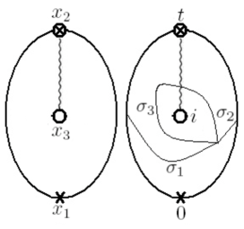
Figure 1: The field theory diagram and the dual graph. The solid line includes a propagator in the fundamental representation which becomes a boundary on the worldsheet. Big $X$’s represent $\bar{\Psi}\Psi$ insertions and circles represent $\Phi$ insertions.

We fix the interior insertion at $i$ and the boundary insertion at $0$. We choose the boundary insertion fixed at $0$ to be the one not connected to the interior vertex. The position of the remaining boundary insertion will be denoted by $t$. A general quadratic differential of the correct form with a double zero is given by

$$q=\phi(dz)^{2}=\frac{a(z-k)^{2}\left(z-\bar{k}\right)^{2}}{z^{2}(z-i)^{2}(z+i)^{2}(z-t)^{2}}(dz)^{2}.$$ (1)

We demand $\Im(k)>0$ in all expressions. Notice that we have placed an image charge at $-i$ and that $q$ has the symmetry $\phi(\bar{z})=\bar{\phi}(z)$. We label the residues according to their positions by $p_{z}$ and demand: $p_{i}=p_{-i}$. The fact that the dual graph has an order $4$ vertex, which is the same thing as saying that the differential has a double zero, imposes an additional constraint on the residues: $p_{t}=p_{0}+2p_{i}$. The differential in terms of these residues is:

$$q=\left[\frac{i}{2\pi}\frac{\left(p_{0}t+2p_{i}t\right)z^{2}+\left(2p_{i}\right)z+p_{0}t}{z(z-i)(z+i)(z-t)}\right]^{2}(dz)^{2}.$$ (2)

There are double zeros at:

$$k,\bar{k}=\frac{-p_{i}\pm\sqrt{p_{i}^{2}-p_{0}^{2}t^{2}-2p_{0}p_{i}t^{2}}}{p_{0}t+2p_{i}t},$$ (3)

only one of which is inside our area of interest $\Im(z)>0$. Note that in order to get the correct graph we need $k$ and $\bar{k}$ to be a complex conjugate pair. This means restricting the integration over the $p_{z}$ and $t$ to where $\sqrt{p_{i}^{2}-p_{0}^{2}t^{2}-2p_{0}p_{i}t^{2}}$ is imaginary or equivalently $p_{i}^{2}-p_{0}^{2}t^{2}-2p_{0}p_{i}t^{2}<0$. The invariant line element is:

$$\sqrt{\phi}dz=\frac{i}{2\pi}\frac{\left(p_{0}t+2p_{i}t\right)z^{2}+\left(2p_{i}\right)z+p_{0}t}{z(z-i)(z+i)(z-t)}dz,$$ (4)

which we will integrate to get the undetermined length in the critical graph:

$$\int\sqrt{\phi}dz=\frac{i}{2\pi}\left(-p_{0}\log(z)+(p_{0}+2p_{i})\log(z-t)-p_{i}\log\left(z^{2}+1\right)\right).$$ (5)

The integrated length along a specific line between the two zeros (drawn in figure 2) is:

$$l=\int_{k}^{\bar{k}}\sqrt{\phi}dz=\frac{p_{0}}{\pi}\arg(k)-\frac{p_{0}+2p_{i}}{\pi}\arg(k-t)+\frac{p_{i}}{\pi}\arg(k^{2}+1).$$ (6)

Note that $l$ is not one of the Strebel lengths, but that all Strebel lengths can be derived from $l$ and the residues $p_{z_{i}}$ (see figure 2). Define the quotient $x\equiv\frac{p_{i}}{p_{0}}$, and a few expressions:

1. $A\equiv x-i{\sqrt{t^{2}+2t^{2}x-x^{2}}}$

2. $B\equiv-x-t^{2}\left(1+2x\right)-i{\sqrt{t^{2}+2t^{2}x-x^{2}}}$

3. $C\equiv x+t^{2}\left(1+2x\right)+i{\sqrt{t^{2}+2t^{2}x-x^{2}}}$

so that :

$$l=\frac{ip_{0}}{2\pi}\left[\left(\log A-\log\bar{A}\right)+(2x+1)\left(\log B-\log\bar{B}\right)+x\left(\log C-\log\bar{C}\right)\right].$$ (7)

Notice that the expression is always real in the region of integration which is where the two zeros are a conjugate pair and our symmetry $\phi(\bar{z})=\bar{\phi}(z)$ holds, implying $t^{2}+2t^{2}x-x^{2}\geq 0$.

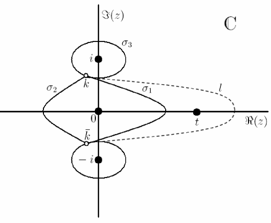
Figure 2: The critical graph of the Strebel differential. The solid balls mark the positions of insertions. The small circles mark the positions of the zeros of the differential.

Let us write the field theory expression for the amplitude. We use position space Schwinger parameters $\sigma_{i}$ (assuming a single contraction of massless scalar fields along each line), such that the correlation function is given by

$$G(x_{1},x_{2},x_{3})=(const)\int_{0}^{\infty}\prod_{i=1}^{3}d\sigma_{i}e^{-(\sigma_{1}+\sigma_{2})(x_{1}-x_{2})^{2}-\sigma_{3}(x_{2}-x_{3})^{2}}.$$ (8)

Finally, we are ready to insert the data from the critical graph of the Strebel differential into this equation by making the identification: $\text{(Strebel length)}\equiv\sigma_{i}$. Let us write the appropriate dictionary in terms of our worldsheet moduli (see figure 2 for the edges corresponding to each $\sigma_{i}$) :

$$\sigma_{1}=\frac{p_{0}+2p_{i}-l}{2},\qquad\sigma_{2}=\frac{l-2p_{i}}{2},\qquad\sigma_{3}=p_{i}.$$ (9)

We now change variables from $\sigma_{i}$ to $\left(p_{0},x,t\right)$. The determinant of the transformation matrix (the Jacobian) is:

$$\textit{J}=\left|\frac{\partial\left(\sigma_{1},\sigma_{2},\sigma_{3}\right)}{\partial\left(p_{0},x,t\right)}\right|=\left|\frac{\partial\left(\sigma_{1},\sigma_{2},\sigma_{3}\right)}{\partial\left(p_{0},p_{i},t\right)}\frac{\partial\left(p_{0},p_{i},t\right)}{\partial\left(p_{0},x,t\right)}\right|=\frac{p_{0}^{2}{\sqrt{t^{2}+2t^{2}x-x^{2}}}}{4\pi t+4\pi t^{3}}\geq 0.$$ (10)

We will integrate only over $t>0$ and multiply the result by $2$. The correlator is:

$$G(x_{1},x_{2},x_{3})= 2(const)\int dtdp_{0}dx\frac{p_{0}^{2}{\sqrt{t^{2}+2t^{2}x-x^{2}}}}{4\pi t+4\pi t^{3}}e^{-p_{0}\left(\frac{1}{2}(x_{1}-x_{2})^{2}+x(x_{2}-x_{3})^{2}\right),}$$ (11)

where the bounds of integration are:

$$p_{0}\in(0,\infty),\qquad t\in(0,\infty),\qquad x\in(0,t^{2}+\sqrt{t^{2}+t^{4}}).$$ (12)

Performing the integration over $p_{0}$ gives:

$$G(x_{1},x_{2},x_{3})= 32(const)\int dtdx\frac{{\sqrt{t^{2}+2t^{2}x-x^{2}}}}{4\pi t+4\pi t^{3}}\frac{1}{((x_{1}-x_{2})^{2}+2x(x_{2}-x_{3})^{2})^{3}.}$$ (13)

We can now do the final integration over $x$. Define:

$$K_{123}\equiv\frac{\left(x_{3}-x_{2}\right)^{2}}{\left(x_{2}-x_{1}\right)^{2}}$$ (14)

$$r\equiv 2(K_{123}-1)\left(t^{2}+\sqrt{t^{4}+t^{2}}\right)-1,\qquad q\equiv 2K_{123}\left(t^{2}+\sqrt{t^{4}+t^{2}}\right)+1$$ (15)

then

$$G(x_{1},x_{2},x_{3})=\frac{(const)}{\left(x_{1}-x_{2}\right)^{6}}\int_{0}^{\infty}dt\frac{(q-r-2)\left(\sqrt{qr}(q+r)-(q-r)^{2}\tanh^{-1}\left(\sqrt{\frac{r}{q}}\right)\right)}{\pi(qr)^{3/2}\left(t^{2}+1\right)}$$ (16)

which is our final expression of the correlator as a function of the modulus $t$. We do not have any particular insight into the meaning of this expression.

Next, in order to compute the OPE of the two open string vertices we expand around $t=0$. The first few terms of the integrand (ignoring the $(const)$ from the correlator) are:

$$G(x_{1},x_{2},x_{3})=\frac{2}{\left(x_{2}-x_{1}\right)^{6}}\,t+\frac{\left(8-16\,K_{123}\right)}{\pi\left(x_{2}-x_{1}\right)^{6}}t^{2}+\frac{12\,\left(K_{123}-1\right)\,K_{123}}{\left(x_{2}-x_{1}\right)^{6}}\,t^{3}+{\text{O}(t)^{4}}.$$ (17)

Note that the power series involves integer powers of $t$, suggesting operators of dimension $\Delta=3,4,...$ appearing in the OPE. Note also that, with the exception of the leading term, all odd orders in $t$ vanish at $K_{123}=1$ ($r=-1$) and all even orders at $K_{123}=\frac{1}{2}$ ($r=-q$). Also the expression is non-singular in $K_{123}$ so only positive powers of $K_{123}$ appear in the expansion. For large $K_{123}$ the $N^{\prime}th$ order in $t$ seems to scale as $K_{123}^{N-1}$ (for all N not just the ones shown). The $K_{123}\rightarrow 0$ limit, which should be singular if we consider the full correlator, is actually regular for each term in the $t$ expansion, and the divergence comes from summing the series.

Integrating the complete answer on the range $t\in(0,\infty)$ we of course recover the expected correlator:

$$G(x_{1},x_{2},x_{3})=\frac{(const)}{K_{123}\left(x_{1}-x_{2}\right)^{6}}=(const)\frac{1}{\left(x_{2}-x_{1}\right)^{4}\left(x_{3}-x_{2}\right)^{2}}$$ (18)

Next, we wish to consider more general correlators such as

$$G(x_{1},x_{2},x_{3})=\left\langle\bar{\Psi}\Phi^{n_{1}}\Psi{\left(x_{1}\right)}\bar{\Psi}\Phi^{n_{2}}\Psi{\left(x_{2}\right)}tr\left(\Phi^{n_{3}}{\left(x_{3}\right)}\right)\right\rangle$$ (19)

(with $n_{2}=n_{1}+n_{3}$) which also get contributions from the same skeleton graph. In order to analyze the OPE in this more general case we analyze the leading order $t$-dependence of the various lines in the diagram. We change variables to $y\equiv\frac{x}{t^{2}+\sqrt{t^{2}+t^{4}}}$. The range of $y$ is from $0$ to $1$. The three lines are now:

1. $\sigma_{1}=\frac{p_{0}}{2}+O(t)$

2. $\sigma_{2}=\frac{p_{0}}{4\pi}\left(2\sqrt{1-y^{2}}-2y\arccos\left(y\right)\right)t+O(t^{2})$

3. $\sigma_{3}=p_{0}yt+O(t^{2})$

Adding lines to the diagram, by adding $\Phi$’s to the operators in our field theory correlation function, changes the leading order $t$ dependence. An additional line homotopic to $\sigma_{2}$ or $\sigma_{3}$ will increase the leading power by $1$. Additional lines homotopic to $\sigma_{1}$, which is the line separating the converging insertions, do not change the leading order behavior. For example, the leading term after adding a $\sigma_{2}$ line is:

$$G(x_{1},x_{2},x_{3})\approx\frac{64-12\pi}{3\pi^{2}\left(x_{2}-x_{1}\right)^{8}}t^{2}.$$ (20)

We can write down the result for the leading power appearing in the OPE as a function of the number of adjoint contractions between the various points. Let $L_{1}$ be the number of adjoint contractions between $x_{1}$ and $x_{2}$ on the OPE side, and $L_{2}$ on the other side, and let $L_{3}$ be the number of adjoint contractions between $x_{2}$ and $x_{3}$. Then, the leading order in the $t\rightarrow 0$ OPE is:

$$G(x_{1},x_{2},x_{3})_{t\rightarrow 0}\sim t^{L_{2}+L_{3}}$$ (21)

We can also analyze the leading order behavior in the $t\rightarrow 0$ limit as a function of the operators we insert in the field theory correlator (19) described above. The two sets are related by:

$$n_{1}=L_{1}+L_{2},\qquad n_{2}=L_{1}+L_{2}+L_{3},\qquad n_{3}=L_{3}.$$ (22)

The lowest order contribution to the OPE with given $\{n_{i}\}$ will come from loading all possible lines on the $\sigma_{1}$ side, taking $L_{2}=0$, giving

$$G(x_{1},x_{2},x_{3})_{t\rightarrow 0}\sim t^{n_{3}},$$ (23)

meaning that the dimension of the leading operator contributing to the OPE of the operators dual to $\bar{\Psi}\Phi^{n_{1}}\Psi$ and $\bar{\Psi}\Phi^{n_{2}}\Psi$ in this diagram is $n_{3}+2=n_{2}-n_{1}+2$.

4 A four-point function example

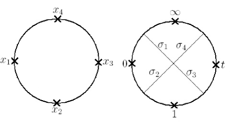
Figure 3: The field theory diagram and the dual graph of the 4 point correlator. The four solid lines form the boundary of a disk.

In this section we evaluate the four point correlator shown in figure 3, which corresponds in the field theory to a correlator such as $\langle\bar{\Psi}\Psi\left(x_{1}\right)\bar{\Psi}\Psi\left(x_{2}\right)\bar{\Psi}\Psi\left(x_{3}\right)\bar{\Psi}\Psi\left(x_{4}\right)\rangle$. The dual line graph describes a disk with four boundary insertions. Our conformal Killing group is again $SL\left(2,\mathbb{R}\right)$. We use this symmetry to fix the positions of three of the boundary insertions at $0$, $1$ and $\infty$. Notice that the fixing does not change the cyclic order of the insertions, which has to be summed over to compute the full correlator.

Again, the dual graph implies that the Strebel differential must have a double zero. A general quadratic differential of the correct form with a double zero is :

$$q=\phi(dz)^{2}=\frac{a(z-k)^{2}(z-\bar{k})^{2}}{z^{2}(z-1)^{2}(z-t)^{2}}(dz)^{2}.$$ (24)

We have one relation between the residues:

$$p_{0}+p_{t}=p_{\infty}+p_{1},$$ (25)

where we have assumed a cyclic order such that $t>1$. The differential in terms of the residues is:

$$q=\left[\frac{1}{2\pi i}\frac{p_{\infty}z^{2}+(-p_{\infty}+p_{1}(t-1)-p_{0}t)z+p_{0}t}{z(z-1)(z-t)}\right]^{2}(dz)^{2},$$ (26)

which has double zeros at:

$$k,\bar{k}=\frac{1}{2p_{\infty}}\left(p_{1}+p_{\infty}+t(p_{0}-p_{1})\pm\sqrt{(p_{1}+p_{\infty}+t(p_{0}-p_{1}))^{2}-4p_{0}p_{\infty}t}\right)$$ (27)

To find the range of integration we demand that $\Im(k)>0$ and the two zeros form a conjugate pair. This gives the constraint:

$$(p_{1}+p_{\infty}+t(p_{0}-p_{1}))^{2}-4p_{0}p_{\infty}t\leq 0,$$ (28)

or equivalently:

$$t-x+tx-2\sqrt{t^{2}x-tx}\leq y\leq t-x+tx+2\sqrt{t^{2}x-tx},$$ (29)

where we have defined the ratios $x\equiv\frac{p_{1}}{p_{0}},y\equiv\frac{p_{\infty}}{p_{0}}$.

The invariant line element is:

$$\sqrt{\phi}dz=\frac{1}{2\pi i}\frac{p_{\infty}z^{2}+(-p_{\infty}+p_{1}(t-1)-p_{0}t)z+p_{0}t}{z(z-1)(z-t)}dz,$$ (30)

and the integrated metric is :

$$\int\sqrt{\phi}dz=\frac{1}{2\pi i}(p_{0}\log(z)-p_{1}\log(z-1)+\left(p_{\infty}+p_{1}-p_{0}\right)\log(z-t)).$$ (31)

The integrated length along one of the edges in the graph (see figure 4) is:

$$l=\int_{k}^{\bar{k}}\sqrt{\phi}dz=\frac{p_{0}}{\pi}\arg(k)-\frac{p_{1}}{\pi}\arg(k-1)+\frac{\left(p_{\infty}+p_{1}-p_{0}\right)}{\pi}\arg(k-t).$$ (32)

We define a few more functions:

1. $\tilde{A}\equiv t+x-tx+y+{\sqrt{-4ty+{\left(t+x-tx+y\right)}^{2}}},$

2. $\tilde{B}\equiv t+x-tx-y-{\sqrt{-4ty+{\left(t+x-tx+y\right)}^{2}}},$

3. $\tilde{C}\equiv t+x-tx+y-2ty+{\sqrt{-4ty+{\left(t+x-tx+y\right)}^{2}}},$

such that :

$$l=\frac{ip_{0}}{2\pi}\left[\left(\log\tilde{A}-\log\bar{\tilde{A}}\right)-x\left(\log\tilde{B}-\log\bar{\tilde{B}}\right)+(x+y-1)\left(\log\tilde{C}-\log\bar{\tilde{C}}\right)\right]$$ (33)

Note that this expression is real in the region of integration.

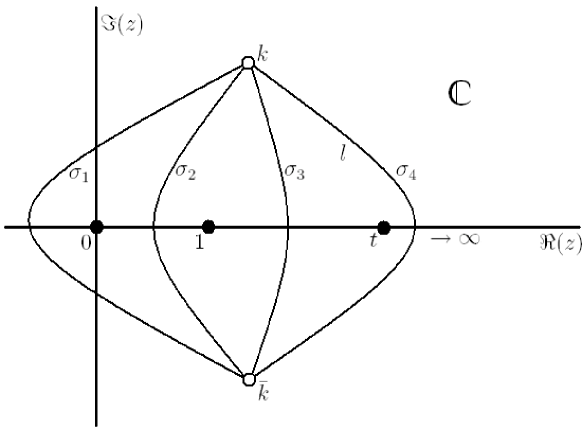
Figure 4: The critical graph of the 4-point Strebel differential.

Next, we construct the dictionary between the $\sigma_{i}$’s and the worldsheet moduli for the regime where $p_{0}+p_{t}=p_{\infty}+p_{1}$:

$$\sigma_{1}=\frac{1}{2}(p_{\infty}-l),\qquad\sigma_{2}=\frac{1}{2}(p_{0}-p_{\infty}+l),\qquad\sigma_{3}=\frac{1}{2}(p_{1}+p_{\infty}-p_{0}-l),\qquad\sigma_{4}=\frac{l}{2}.$$ (34)

The range of integration is

$$t\in(1,\infty),\qquad p_{0}\in(0,\infty),\qquad x\in(0,\infty),$$

$$y\in\left(t-x+tx-2{\sqrt{t^{2}x-tx}},t-x+tx+2{\sqrt{t^{2}x-tx}}\right),$$ (35)

where we have taken into account the support for the $\delta$-function integration $\delta\left(p_{t}-\left(p_{\infty}+p_{1}-p_{0}\right)\right)$. The Jacobian for the change of variables from $\left(\sigma_{1},\sigma_{2},\sigma_{3},\sigma_{4}\right)$ to $\left(p_{0},x,y,t\right)$ is:

$$\textit{J}=\frac{-ip_{0}^{3}}{32}\frac{{\sqrt{{\left(t+x-t\,x+y\right)}^{2}-4ty}}}{\pi\,\left(t-1\right)\,t}.$$ (36)

Note that J is real and positive in the range of integration. Once again we write the field theory expression for the amplitude. Define also $J_{1}$ as the jacobian for the change of variables from $\left(\sigma_{1},\sigma_{2},\sigma_{3},\sigma_{4}\right)$ to $\left(p_{0},p_{1},p_{\infty},t\right)$. The correlator in position space is given by:

$$G(x_{1},x_{2},x_{3},x_{4})=\int_{0}^{\infty}\prod_{i=1}^{4}d\sigma_{i}e^{-\sigma_{1}\left(x_{4}-x_{1}\right)^{2}-\sigma_{2}\left(x_{1}-x_{2}\right)^{2}-\sigma_{3}\left(x_{2}-x_{3}\right)^{2}-\sigma_{4}\left(x_{3}-x_{4}\right)^{2}}$$ (37)

$$=\int dtdp_{0}dp_{1}dp_{\infty}\textit{J}_{1}e^{-\frac{1}{2}\left(p_{\infty}-l\right)\left(x_{4}-x_{1}\right)^{2}-\frac{1}{2}(p_{0}-p_{\infty}+l)\left(x_{1}-x_{2}\right)^{2}-\frac{1}{2}(p_{1}+p_{\infty}-p_{0}-l)\left(x_{2}-x_{3}\right)^{2}-\frac{l}{2}\left(x_{3}-x_{4}\right)^{2}}$$ (38)

$$=\int dtdp_{0}dxdy\textit{J}e^{-\frac{1}{2}\left(yp_{0}-l\right)\left(x_{4}-x_{1}\right)^{2}-\frac{1}{2}(p_{0}-yp_{0}+l)\left(x_{1}-x_{2}\right)^{2}-\frac{1}{2}(xp_{0}+yp_{0}-p_{0}-l)\left(x_{2}-x_{3}\right)^{2}-\frac{l}{2}\left(x_{3}-x_{4}\right)^{2}}.$$ (39)

We perform the $dp_{0}$ integration (which kills the exponent):

$$G(x_{1},x_{2},x_{3},x_{4})=\int dtdxdy\frac{-3i}{16\pi}\frac{{\sqrt{{\left(t+x-t\,x+y\right)}^{2}-4ty}}}{t^{2}-t}$$ (40)

$$\left(\frac{y-\tilde{l}}{2}\left(x_{4}-x_{1}\right)^{2}+\frac{1-y+\tilde{l}}{2}\left(x_{1}-x_{2}\right)^{2}+\frac{x+y-1-\tilde{l}}{2}\left(x_{2}-x_{3}\right)^{2}+\frac{\tilde{l}}{2}\left(x_{3}-x_{4}\right)^{2}\right)^{-4},$$ (41)

where $\tilde{l}\equiv\frac{l}{p_{0}}$ does not depend on $p_{0}$.

We were not able to do the explicit integral over $x$ and $y$ to obtain the full correlation function, but we can analyze it in the two OPE limits $t\rightarrow 1$ and $t\rightarrow\infty$. We switch to the variables:

$$\begin{cases}t\rightarrow 1&u\equiv\frac{t\left(x-1\right)-x-y}{{\sqrt{ty}}},\\ t\rightarrow\infty&u\equiv\frac{y-t+x-tx}{\sqrt{t^{2}x-tx}}.\end{cases}$$ (42)

The ranges of integration are now

$$t\in(1,\infty)\qquad x,y\in(0,\infty)\qquad u\in\left(-2,2\right)$$ (43)

The leading order contributions to the $dt$ integral are now:

$$G(x_{1},x_{2},x_{3},x_{4})\approx\begin{cases}t\rightarrow 1&\int dydu\frac{\left(-3i\right){\sqrt{-4+u^{2}}}y}{\pi{\left(1+u{\sqrt{y}}+y\right)}^{4}{\left(x_{3}-x_{2}\right)}^{8}}\left(t-1\right)^{2}=\frac{3}{8{\left(x_{3}-x_{2}\right)}^{8}}\left(t-1\right)^{2},\\ t\rightarrow\infty&\int dxdu\frac{\left(-3i\right){\sqrt{-4+u^{2}}}x}{\pi{\left(1+u{\sqrt{x}}+x\right)}^{4}{\left(x_{3}-x_{4}\right)}^{8}}\frac{1}{t^{4}}=\frac{3}{8{\left(x_{3}-x_{4}\right)}^{8}}\frac{1}{t^{4}}.\end{cases}$$ (44)

Note the similarity between these expressions. The two OPE limits are of course identical, up to exchanging of the $x_{i}$, from the field theory point of view. On the worldsheet the two limits are connected by the transformation $t\rightarrow\frac{t}{t-1}$, which exchanges $1$ and $\infty$ and keeps $0$ fixed. The difference in the power of the leading order stems from the Jacobian of this transformation, $\frac{1}{(t-1)^{2}}$. The result suggests that the OPE expansion contains operators of worldsheet dimension $\Delta=4,5,..$. We have checked numerically that the final integrated answer scales as: (as is obvious from (37))

$$(const)\frac{1}{\left(x_{2}-x_{1}\right)^{2}\left(x_{3}-x_{2}\right)^{2}\left(x_{4}-x_{3}\right)^{2}\left(x_{1}-x_{4}\right)^{2}}.$$ (45)

We can add additional adjoint lines to this correlator, computing more general correlators of the form

$$G(x_{1},x_{2},x_{3},x_{4})=\left\langle 0\left|\bar{\Psi}\Phi^{n_{1}}\Psi{\left(x_{1}\right)}\bar{\Psi}\Phi^{n_{2}}\Psi{\left(x_{2}\right)}\bar{\Psi}\Phi^{n_{3}}\Psi{\left(x_{3}\right)}\bar{\Psi}\Phi^{n_{4}}\Psi{\left(x_{4}\right)}\right|0\right\rangle.$$ (46)

Note that there are additional diagrams that contribute to this correlator, but we will only be interested in those Feynman diagrams which upon gluing give the diagram of figure 3. Even in this diagram there are different ways to distribute the contractions for given operators. In order to analyze the general OPE we need to compute the scalings of the various edges in the OPE limits, which are given in Table 1.

edge	connects	worldsheet value	$t\rightarrow 1$	$t\rightarrow\infty$
$\sigma_{1}$	$x_{4}\longleftrightarrow x_{1}$	$\frac{1}{2}(p_{\infty}-l)$	$O\left(t-1\right)$	$O\left(\frac{1}{t}\right)$
$\sigma_{2}$	$x_{1}\longleftrightarrow x_{2}$	$\frac{1}{2}(p_{0}-p_{\infty}+l)$	$O\left(t-1\right)$	$O\left(\frac{1}{t}\right)$
$\sigma_{3}$	$x_{2}\longleftrightarrow x_{3}$	$\frac{1}{2}(p_{1}+p_{\infty}-p_{0}-l)$	$O\left(1\right)$	$O\left(\frac{1}{t}\right)$
$\sigma_{4}$	$x_{3}\longleftrightarrow x_{4}$	$\frac{1}{2}l$	$O\left(t-1\right)$	$O\left(1\right)$

Table 1: Edge scaling in the two OPE limits.

Let $L_{i}$ be the number of adjoint contractions between $x_{i}$ and $x_{i+1}$ ($L_{4}$ is between $x_{4}$ and $x_{1}$). Then, the leading orders in the OPE’s are:

$$G(x_{1},x_{2},x_{3},x_{4})\sim\begin{cases}t\rightarrow 1&t^{L_{1}+L_{3}+L_{4}+2},\\ t\rightarrow\infty&\left(\frac{1}{t}\right)^{L_{1}+L_{2}+L_{4}+4}.\end{cases}$$ (47)

In the correlator described above we have :

$$n_{1}=L_{4}+L_{1},\qquad n_{2}=L_{1}+L_{2},\qquad n_{3}=L_{2}+L_{3},\qquad n_{4}=L_{3}+L_{4}.$$ (48)

These must satisfy $n_{1}+n_{3}=n_{2}+n_{4}$ in order to connect all lines. Given this constraint it is always possible to connect at most $\min\left(n_{2},n_{3}\right)$ lines between $x_{2}$ and $x_{3}$, or $\min\left(n_{3},n_{4}\right)$ lines between $x_{3}$ and $x_{4}$. These contractions will contribute to the leading order of the OPE’s:

$$G(x_{1},x_{2},x_{3},x_{4})\sim\begin{cases}t\rightarrow 1&\left(t-1\right)^{\frac{1}{2}\left(n_{1}+n_{4}+|n_{2}-n_{3}|\right)+2}=\left(t-1\right)^{\max\left(n_{1},n_{4}\right)+2},\\ t\rightarrow\infty&\left(\frac{1}{t}\right)^{\max\left(n_{1},n_{2}\right)+4}.\end{cases}$$ (49)

Note that the limit $t\rightarrow 1$ corresponds to the OPE between the vertex operators corresponding to $\bar{\Psi}\Phi^{n_{2}}\Psi{\left(x_{2}\right)}$ and $\bar{\Psi}\Phi^{n_{3}}\Psi{\left(x_{3}\right)}$, while the limit $t\rightarrow\infty$ corresponds to the OPE between the vertex operators corresponding to $\bar{\Psi}\Phi^{n_{3}}\Psi{\left(x_{3}\right)}$ and $\bar{\Psi}\Phi^{n_{4}}\Psi{\left(x_{4}\right)}$.

5 Discussion and conclusions

As was discussed in [12], the worldsheet expressions obtained from this formalism do not realize the space-time conformal symmetry as a local symmetry. In our open string diagrams we can see this already at the level of the 3-point function (16). Of the possible space-time transformations, only the Poincaré and scaling symmetries are locally realized global symmetries of the integrands in the examples. The full conformal symmetry is of course restored after we integrate over all the moduli.

In both examples the leading order contribution to an OPE depended on the multiplicities of all lines not connecting the converging operators. At first sight this is surprising since the OPE should depend on the operators which are converging. However, this can be seen as a manifestation of worldsheet conformal invariance. Consider the convergence of $2$ out of $n$ operators on the boundary (which is present for planar diagrams) or in the interior of a worldsheet. If we assume a large enough conformal group then as the operators come together we may always choose a conformal frame where the converging operators are held fixed, say at $0$ and $1$. It is easy to show that in this frame the rest of the operators converge on each other. The two limits, the one of two operators converging and the one of $n-2$, are thus equivalent. It is not surprising that the OPE computed through this $n$-point diagram will depend on all the multiplicities in the diagram.

The operator product expansions in both examples, and in the general analysis of appendix A, consist of positive integer powers of the separation. This suggests that the operators appearing in the expansion also have positive integer worldsheet dimensions (starting from dimension $3$ in the three point example and dimension $n$ in the general circle diagram of order $n$).

Appendix A The general circle diagram of even order

We can generalize the results of the four-point example of section 4 to determine the OPE’s for the general circle diagram with an even number $n$ of insertions. In these types of diagrams there is only one unknown length to compute. The first fact we will use is that the differential for a circle diagram with an even number of insertions is a perfect square. We will use the same conventions as in the four point example and set the position of one insertion to $z_{1}=0$, another to $z_{2}=1$ and another to $z_{n}=\infty$, and choose the rest of the insertions, $\{z_{3},z_{4},..,z_{n-1}\}$ to lie between $1$ and $\infty$. The invariant line element is now a rational function with a numerator which has two conjugate zeros, $k$ and $\bar{k}$, each with multiplicity $n/2-1$ and a denominator which is the product of $n-1$ distinct monomials:

$$\sqrt{\phi\left(z\right)}dz=\frac{p_{\infty}\left(z-k\right)^{\frac{n}{2}-1}\left(z-\bar{k}\right)^{\frac{n}{2}-1}}{2\pi i\prod_{j=1}^{n-1}\left(z-z_{j}\right)}dz.$$ (50)

This type of function can always be expressed as the sum of rational functions where the denominators are the monomials and the numerators are numbers. The numerators must be the residues and the entire differential is so determined:

$$\sqrt{\phi\left(z\right)}dz=\sum_{j=1}^{n-1}\frac{\left(-1\right)^{j+1}p_{z_{j}}}{2\pi i}\frac{1}{z-z_{j}}dz.$$ (51)

Note the alternating signs needed to ensure that the single residue relation,

$$p_{\infty}=\sum_{i=1}^{n-1}(-1)^{i+1}p_{z_{i}},$$ (52)

holds. The integrated length is just a sum of logarithms which is equivalent to a sum of arguments of $k-z_{i}$ as we showed in the example. The coefficients are just the residues (with alternating signs):

$$l=\int_{k}^{\bar{k}}\sqrt{\phi\left(z\right)}dz=\sum_{j=1}^{n-1}\frac{\left(-1\right)^{j+1}p_{z_{j}}}{\pi}\arg\left(k-z_{j}\right)$$ (53)

We denote the position of the insertion closest to $\infty$ by $t$. We will analyze the scaling of the different components in the calculation as a function of $t$. Notice the residue relation $p_{t}=\sum_{j=1}^{n-2}(-1)^{j}p_{z_{j}}+p_{\infty}$ implies that the factor $p_{\infty}$ appears only in the numerator of the final fraction:

$$\frac{\sum_{j=1}^{n-2}(-1)^{j}p_{z_{j}}+p_{\infty}}{2\pi i}\frac{1}{z-t}.$$ (54)

We take the $n$ parameters of the field theory to be the $n-1$ independent $p_{z_{i}}$ and the modulus $t$. All other position moduli must then be determined as a function of these in order to retain a differential with a single conjugate pair of zeros (one that fits our diagram). Notice that the $t$ scaling of these functions has no bearing on the scaling of the undetermined length $l$. In fact there appears to be no parameter in $l$ that can scale with $t$. This is not completely true since one must still restrict the range of integration of one residue, which we take to be $p_{\infty}$, so that the two zeros form a conjugate pair. Assume that the functions that fix the remaining $z_{i}$, in terms of $t$ and the $p_{z_{i}}$, have been determined. Assume also that we have performed a change of variables so as to fix the $t$-dependent boundaries of integration for $p_{\infty}$, and replaced $p_{\infty}$ with a variable $u$, which does not scale with $t$, and some explicit dependence on $t$ and the other $p_{z_{i}}$. We examine the $t\rightarrow\infty$ limit keeping $p_{z_{i}\neq\infty}$ and $u$ fixed. We assume that we can take this limit inside the various integrations. The numerator for the invariant line element is now a polynomial of the form

$$P(z)=\left(Az^{2}+Bz+C\right)^{\frac{n}{2}-1}.$$ (55)

Some of the coefficients are :

• $\text{coef.}(z^{n-2})=A^{\frac{n}{2}-1},$

• $\text{coef.}(1)=C^{\frac{n}{2}-1},$

• $\text{coef.}(z)=\left(\frac{n}{2}-1\right)BC^{\frac{n}{2}-2}.$

We can write the same coefficients in terms of the $p_{z_{i}}$ and the $z_{i}$ :

• $\text{coef.}(z^{n-2})=p_{\infty},$

• $\text{coef.}(1)=p_{0}\prod_{z_{i}\neq 0}z_{i},$

• $\text{coef.}(z)=\sum_{i=1}^{n-1}(-1)^{i+1}p_{z_{i}}\sum_{j\neq i}\prod_{k\neq i,j}(-z_{k}).$

The condition for getting a pair of conjugate zeros is $B^{2}<4AC$, which we viewed as an equation for the range of $p_{\infty}$. The boundaries of the region of integration obey $B^{2}=4AC$, and we require this to have (non-degenerate) solutions in the large $t$ limit. Denote by $\alpha_{i}$ the scaling of the (fixed) position $z_{i}$ (so that, for $t\gg 1$, $z_{i}\sim t^{\alpha_{i}}$). We demand $\alpha_{i}\geq 0\ \forall i$, otherwise two poles would collide for some finite $t$. Denote by $p$ the scaling of $p_{\infty}$, and by $(a,b,c)$ the scalings of $(A,B,C)$. We can now write equations for the relationships between these scalings:

• $a=\frac{p}{\frac{n}{2}-1}$

• $c=\frac{1+\sum_{i}\alpha_{i}}{\frac{n}{2}-1}$

• $B^{2}=4AC\Rightarrow b=\frac{1}{2}(a+c)=\frac{1+p+\sum_{i}\alpha_{i}}{n-2}$

• $b+(\frac{n}{2}-2)c=max\{\sum_{i}\alpha_{i}+1,\sum_{i}\alpha_{i}+p\}$

with the final equation coming from considering the largest possible scaling for the coefficient of $z$. We can show that these imply $p=1$, since :

$$\begin{cases}p>1&\Rightarrow\sum_{i}\alpha_{i}+p=\frac{1+p+\sum_{i}\alpha_{i}}{n-2}+(\frac{n}{2}-2)\left(\frac{1+\sum_{i}\alpha_{i}}{\frac{n}{2}-1}\right)\Rightarrow\\ &p=1-\frac{\sum_{i}\alpha_{i}}{n-3}\leq 1\ (contradiction),\\ p<1&\Rightarrow\sum_{i}\alpha_{i}+1=\frac{1+p+\sum_{i}\alpha_{i}}{n-2}+(\frac{n}{2}-2)\left(\frac{1+\sum_{i}\alpha_{i}}{\frac{n}{2}-1}\right)\Rightarrow\\ &p=1+\sum_{i}\alpha_{i}\geq 1\ (contradiction).\end{cases}$$ (56)

This in turn implies $\alpha_{i}=0\ \forall i$ and $a=b=c=\frac{2}{n-2}$. The second equality tells us that the positions of the zeros, $k$ and $\bar{k}$, do not scale with $t$.

Given this we are in exactly the same situation as we were for the $4$ point example. For $t\rightarrow\infty$ we have $l\sim p_{\infty}$. Note that for $t\gg 1$ $\frac{1}{\pi}\arg(k-t)\approx 1$. All other lines in the diagram are expressions of the type $(p_{\infty}+f(\{p_{z}\}_{z\neq\infty}))-l$ and will therefore not scale with $t$. The last thing to consider is the integration over $p_{0}$. This kills the exponent and brings the expression $-\sum_{s=1}^{n}\tilde{\sigma}_{s}\left(x_{s(1)}-x_{s(2)}\right)^{2}$, $\tilde{\sigma}_{s}\equiv\sigma_{s}/p_{0}$ into the denominator. The power to which this expression is raised is set by the dimension of the correlator. The initial power is $n$ and adding one line adds one power. All the $\sigma_{i}$, with the exception of the one associated with $l$, contain $p_{\infty}-l$ and do not scale with $t$. The denominator therefore scales as $t^{n}$. We can follow the changes of variables to show that the product of the various Jacobians does not scale with $t$. The leading order in the OPE with $t\rightarrow\infty$ is therefore $\left(\frac{1}{t}\right)^{n}$ which is consistent with our analysis of the four point example. Thus, the lowest dimension operator contributing to the OPE has dimension $n$. Adding lines connecting the converging operators, the line associated with $l$, does not change this as $l$ scales linearly and the power to which the linearly scaling expression in the denominator is raised increases by one. Adding any other line decreases the leading power by one, as these lines do not scale with $t$ but have the same effect on the denominator.

We can probably do a similar analysis for even circle correlators with interior insertions connected to one of the boundary insertions (like in the three-point example, but with more boundary and interior insertions). There would be no restriction on the number of interior insertions, as each contributes two to the orders of the two zeros $k$ and $\bar{k}$. Other types of diagrams whose differentials are perfect squares may also be possible to analyze in general.

References

- [1] R. Gopakumar, “From free fields to AdS,” Phys. Rev. D 70, 025009 (2004) [arXiv:hep-th/0308184].
- [2] R. Gopakumar, “From free fields to AdS. II,” Phys. Rev. D 70, 025010 (2004) [arXiv:hep-th/0402063].
- [3] R. Gopakumar, “From free fields to AdS. III,” Phys. Rev. D 72, 066008 (2005) [arXiv:hep-th/0504229].
- [4] R. Gopakumar, “Free field theory as a string theory?,” Comptes Rendus Physique 5, 1111 (2004) [arXiv:hep-th/0409233]. K. Furuuchi, “From free fields to AdS: Thermal case,” Phys. Rev. D 72, 066009 (2005) [arXiv:hep-th/0505148]. J. R. David and R. Gopakumar, “From spacetime to worldsheet: Four point correlators,” arXiv:hep-th/0606078.
- [5] J. M. Maldacena, “The large N limit of superconformal field theories and supergravity,” Adv. Theor. Math. Phys. 2, 231 (1998) [Int. J. Theor. Phys. 38, 1113 (1999)] [arXiv:hep-th/9711200]. S. S. Gubser, I. R. Klebanov and A. M. Polyakov, “Gauge theory correlators from non-critical string theory,” Phys. Lett. B 428, 105 (1998) [arXiv:hep-th/9802109]. E. Witten, “Anti-de Sitter space and holography,” Adv. Theor. Math. Phys. 2, 253 (1998) [arXiv:hep-th/9802150]. O. Aharony, S. S. Gubser, J. M. Maldacena, H. Ooguri and Y. Oz, “Large N field theories, string theory and gravity,” Phys. Rept. 323, 183 (2000) [arXiv:hep-th/9905111].
- [6] K. Strebel, “Quadratic Differentials,” Springer-Verlag (1980).
- [7] N. Moeller, “Closed Bosonic String Field Theory At Quartic Order,” JHEP 0411, 018 (2004) [arXiv:hep-th/0408067].
- [8] M. Kontsevich, “Intersection theory on the moduli space of curves and the matrix Airy function,” Commun. Math. Phys. 147, 1 (1992). D. Zvonkine, “Strebel differentials on stable curves and Kontsevich’s proof of Witten’s conjecture,” [math.AG/0209071].
- [9] J. D. Bjorken and S. D. Drell, “Relativistic Quantum Fields”, (McGraw Hill, 1965).
- [10] B. Zwiebach, “Minimal Area Problems And Quantum Open Strings,” Commun. Math. Phys. 141, 577 (1991). B. Zwiebach, “A Proof that Witten’s open string theory gives a single cover of moduli space,” Commun. Math. Phys. 142, 193 (1991). M. Wolf and B. Zwiebach, “The Plumbing Of Minimal Area Surfaces,” arXiv:hep-th/9202062.
- [11] G. ’t Hooft, “A Planar Diagram Theory For Strong Interactions,” Nucl. Phys. B 72, 461 (1974).
- [12] O. Aharony, Z. Komargodski and S. S. Razamat, “On the worldsheet theories of strings dual to free large N gauge theories,” JHEP 0605, 016 (2006) [arXiv:hep-th/0602226].
- [13] M. Mulase and M. Penkava ”Ribbon Graphs, Quadratic Differentials on Riemann Surfaces, and Algebraic Curves Defined over ”, math-ph/9811024