Photon and dilepton production in supersymmetric Yang-Mills plasma

Abstract

By weakly gauging one of the $U(1)$ subgroups of the $R$-symmetry group, $\mathcal{N}\,{=}\,4$ super-Yang-Mills theory can be coupled to electromagnetism, thus allowing a computation of photon production and related phenomena in a QCD-like non-Abelian plasma at both weak and strong coupling. We compute photon and dilepton emission rates from finite temperature $\mathcal{N}\,{=}\,4$ supersymmetric Yang-Mills plasma both perturbatively at weak coupling to leading order, and non-perturbatively at strong coupling using the AdS/CFT duality conjecture. Comparison of the photo-emission spectra for $\mathcal{N}\,{=}\,4$ plasma at weak coupling, $\mathcal{N}\,{=}\,4$ plasma at strong coupling, and QCD at weak coupling reveals several systematic trends which we discuss. We also evaluate the electric conductivity of $\mathcal{N}\,{=}\,4$ plasma in the strong coupling limit, and to leading-log order at weak coupling. Current-current spectral functions in the strongly coupled theory exhibit hydrodynamic peaks at small frequency, but otherwise show no structure which could be interpreted as well-defined thermal resonances in the high-temperature phase.

I Introduction

Any thermal medium composed of electrically charged particles emits photons. The energy spectrum of the produced photons depends on the details of the system: the spectrum is Planckian when the photons are in thermal equilibrium, and deviates from it when they are not. The quark-gluon plasma (QGP) produced in heavy ion collisions is expected to be optically thin, because of its limited extent and the small value of the electromagnetic coupling $\alpha_{\rm\scriptscriptstyle EM}$. Therefore, a photon, once emitted, should stream through the QCD plasma virtually without subsequent interaction photons-rhic . In such a situation, the photon spectrum will have little to do with the black-body distribution, but may instead give valuable information about the properties of the medium. For instance, while the experimental results RHIC_photon1 ; RHIC_photon2 for photon production at RHIC are currently consistent with pion decay plus prompt photons produced by the initial scattering of the partons from the two nuclei Vogelsang , there is room for photons produced in the hot plasma.

While prompt photons really are perturbative, and pion decay photons can be calibrated from other hadronic signals, the most interesting signal, photon production from the medium, suffers from the usual problem that we only have weak coupling calculations AMY3 for QGP photon production, despite the fact that the medium is probably strongly coupled. Therefore, any guidance on the behavior of photon production as a function of coupling would be useful, even if it comes from an analogue theory which is not quite real QCD. With this in mind, we will calculate photon production in $\mathcal{N}\,{=}\,4$ supersymmetric Yang-Mills theory, where strong coupling techniques exist.

Consider a field theory in thermal equilibrium, and let the photon interaction with matter be of the form $eJ^{\rm\scriptscriptstyle EM}_{\mu}A^{\mu}$, where the electromagnetic coupling $e$ is so small that the photons are not rescattered and thermalized. If $\Gamma_{\gamma}$ denotes the number of photons emitted per unit time per unit volume, then to leading order in $e$ the rate is given by Le-Bellac

$$d\Gamma_{\gamma}=\frac{d^{3}k}{(2\pi)^{3}}\frac{e^{2}}{2|{\bm{k}}|}\;\eta^{\mu\nu}C^{<}_{\mu\nu}(K)\Big{|}_{k^{0}=|{\bm{k}}|}\ ,$$ (1)

where

$$C^{<}_{\mu\nu}(K)=\int\!d^{4}X\>e^{-iK\cdot X}\>\langle J^{\rm\scriptscriptstyle EM}_{\mu}(0)J^{\rm\scriptscriptstyle EM}_{\nu}(X)\rangle$$ (2)

is the Wightman function of electromagnetic currents, and the expectation value is taken in the thermal equilibrium state. Here $\eta_{\mu\nu}={\rm diag}({-}{+}{+}{+})$ is the Minkowski metric, and $K\equiv(k^{0},{\bm{k}})$ is a null 4-vector whose time component is fixed by the on-shell condition $k^{0}=|{\bm{k}}|$. The Wightman correlator (2), in thermal equilibrium, is related to the spectral density,

$$C^{<}_{\mu\nu}(K)=n_{\rm b}(k^{0})\,\chi_{\mu\nu}(K)\,,$$ (3)

where $n_{\rm b}(k^{0})=1/(e^{\beta k^{0}}{-}1)$ is the usual Bose-Einstein distribution function, and $\chi_{\mu\nu}(K)$ is the spectral density, proportional to the imaginary part of the retarded current-current correlation function,

$$\chi_{\mu\nu}(K)=-2\,{\rm Im}\,C^{\rm ret}_{\mu\nu}(K)\,.$$ (4)

If one also adds to the theory massive fermions which carry only electric charge (“leptons”), then the thermal system will also emit these leptons, produced by virtual photon decay. The same electromagnetic current-current correlation function, evaluated for timelike momenta, gives the rate of lepton pair production for each such lepton species Le-Bellac :

$$d\Gamma_{\ell\bar{\ell}}=\frac{d^{4}K}{(2\pi)^{4}}\,\frac{e^{2}\,e_{\ell}^{2}}{6\pi|K^{2}|^{5/2}}\>\Theta(k^{0})\Theta(-K^{2}{-}4m^{2})\,[-K^{2}{-}{4m^{2}}]^{1/2}\,(-K^{2}{+}{2m^{2}})\;\eta^{\mu\nu}C^{<}_{\mu\nu}(K)\,.$$ (5)

Here $e_{\ell}$ is the electric charge of the lepton, $m$ is lepton mass, and the correlator $C^{<}_{\mu\nu}(K)$ is evaluated at the timelike momentum of the emitted particle pair. [$\Theta(x)$ denotes a unit step function.] Expressions (1) and (5) for the production rates are true to leading order in the electromagnetic couplings $e$ and $e_{\ell}$, but are valid non-perturbatively in all other interactions.

The electrical conductivity $\sigma$ of the medium is also determined by the current-current correlator, specifically its zero-frequency limit at vanishing three-momentum,

$$\sigma=\lim_{k^{0}\to 0}\frac{e^{2}}{6T}\>\eta^{\mu\nu}C_{\mu\nu}^{<}(k^{0},{\bm{k}}{=}0)\,.$$ (6)

An equally valid alternative expression relates the conductivity to the the small frequency limit of the correlator for lightlike momenta,

$$\sigma=\lim_{k^{0}\rightarrow 0}\frac{e^{2}}{4T}\>\eta^{\mu\nu}C^{<}_{\mu\nu}(K)\Big{|}_{|{\bm{k}}|=k^{0}}\,.$$ (7)

This form, which will be useful in our discussion of the photon production rate, follows from the Ward identity $K^{\mu}C^{<}_{\mu\nu}(K)=0$ combined with the diffusive nature of the hydrodynamic pole in the correlator.

Both photon and dilepton production rates have previously been calculated in QCD in perturbation theory to leading order in $\alpha_{\rm s}$ [i.e., up to relative corrections suppressed by powers of $\alpha_{\rm s}$] AMY3 ; rates-pert2 . There are also non-perturbative lattice estimates of the dilepton emission rate at zero three-momentum rates-lattice , and of the electric conductivity Gupta , based on attempts to fit the Euclidean correlator using parameterized forms of the spectral density. Reports of lattice studies of current-current spectral functions at non-zero momentum have appeared recently hep-lat/0607012 . (However, the results of these efforts to extract real-time physics from Euclidean lattice simulations are quite sensitive to the assumptions made about the form of the spectral density. Assessing the reliability of these results is not easy; see, for example, Ref. rates-review .)

In this paper, we calculate photon and dilepton production rates in $SU(N_{\rm c})$, $\mathcal{N}\,{=}\,4$ supersymmetric Yang-Mills (SYM) theory at finite temperature and zero chemical potential, at both weak and strong coupling. This theory, at non-zero temperature, mimics many features of high-temperature QCD. It is a non-Abelian plasma which happens to have adjoint representation fermions and scalars instead of fundamental representation quarks. Despite this difference in matter field content, thermal SYM theory exhibits deconfinement, Debye screening, area-law behavior of spatial Wilson loops, and a finite static correlation length, just like hot QCD. But unlike QCD, real-time thermal properties of $\mathcal{N}\,{=}\,4$ SYM theory can be studied analytically at strong coupling. Consequently, in SYM theory one may calculate, reliably, interesting physical observables at both weak and strong coupling. In particular, the calculation of thermal spectral functions in strongly coupled SYM theory is vastly simpler than the corresponding problem in strongly coupled QCD. Full spectral functions of the energy-momentum tensor, at strong coupling, were calculated recently in Refs. spectral ; derek , explicitly showing that strongly coupled SYM theory behaves much more like a liquid, rather than a weakly interacting gas of quasi-particles. At the same time, weak-coupling calculations of the photon emission rates in SYM theory are qualitatively similar to those in QCD, and detailed comparison of the results can shed light on the degree to which thermal QCD can be quantitatively modeled by $\mathcal{N}\,{=}\,4$ SYM theory.

Our paper is organized as follows. In section II we discuss how to couple the degrees of freedom of $\mathcal{N}\,{=}\,4$ SYM theory to electromagnetism. In section III we calculate the trace of the spectral function $\chi^{\mu}_{\ \mu}(K)\equiv\eta^{\mu\nu}\chi_{\mu\nu}(K)$ in strongly coupled SYM theory for arbitrary momenta. The behavior of the spectral functions at small frequencies is in complete agreement with the prediction of linear response for hydrodynamic fluctuations of the conserved charge density. We find a finite result, $\sigma=e^{2}N_{\rm c}^{2}T/16\pi$, for strong coupling limit of the electric conductivity of $\mathcal{N}\,{=}\,4$ SYM theory. In section IV we compute the current-current spectral function in weakly coupled SYM theory, for both timelike and lightlike momenta, for frequencies large compared to $\lambda^{2}\,T$, which is the scale where hydrodynamic effects become important. (Here $\lambda\equiv g^{2}N_{\rm c}\,$ is the ’t Hooft coupling.) This weak-coupling analysis generalizes the corresponding calculation for QCD performed by Arnold, Moore and Yaffe AMY3 . In the final section V we compare the photon emission spectra for SYM and QCD at weak coupling, and SYM at strong coupling, and discuss the relevant lessons which can be drawn. We find that the weak-coupling behavior of SYM is quite similar to that of QCD provided one compares the theories at the same values of thermal masses, rather than equal values of ’t Hooft coupling (although SYM theory has somewhat more soft photons relative to hard photons in comparison with QCD). The strongly coupled theory has a greater photon production rate at large momentum, relative to the weakly coupled theory, but less production at small momenta ($k\ll\lambda^{2/3}\,T$). The production of large mass dilepton pairs is essentially identical between the weakly and strongly coupled theories.

II Coupling $\mathcal{N}\,{=}\,4$ super-Yang-Mills to electromagnetism

The field content of $\mathcal{N}\,{=}\,4$ SYM theory consists of $SU(N_{\rm c})$ gauge bosons, plus four Weyl fermions $\psi_{p}$ and six real scalars $\phi_{pq}\equiv-\phi_{qp}$, $p,q=1,\cdots,4$, transforming in the adjoint representation of $SU(N_{\rm c})$. The theory has an anomaly free global $SU(4)$ $R$-symmetry, under which the fermions transform in the 4 and the scalars in the ${\bf 6}$. To model electromagnetic interactions, we add to the theory a $U(1)$ gauge field coupled to the conserved current corresponding to a $U(1)$ subgroup of the $SU(4)$ $R$-symmetry.

We will choose the $U(1)$ subgroup generated by $t^{3}\equiv{\rm diag}(\frac{1}{2},-\frac{1}{2},0,0)$, under which two of the Weyl fermions have charge $\pm{\textstyle{\frac{1}{2}}}$ and two complex scalars have charge ${\textstyle{\frac{1}{2}}}$. The associated conserved current is

$$J^{\rm EM}_{\mu}\equiv\frac{1}{e}\frac{\delta S_{\rm int}}{\delta A^{\mu}}={\textstyle{\frac{1}{2}}}\Big{[}\psi_{1}^{a\dagger}\bar{\sigma}_{\mu}\psi_{1}^{a}-\psi_{2}^{a\dagger}\bar{\sigma}_{\mu}\psi_{2}^{a}+\sum_{p=3,4}\phi_{1p}^{a\dagger}(-i\vec{D}_{\mu}+i\!\stackrel{{\,{}_{\leftarrow}}}{{D}}_{\mu})\phi_{1p}^{a}\Big{]}\,.$$ (8)

A summation over the $SU(N_{\rm c})$ group index $a$ is implied in Eq. (8). The covariant derivative $D_{\mu}$ acting on the scalars involves both the $SU(N_{\rm c})$ gauge fields and the $U(1)$ electromagnetic potential $A_{\mu}$ (with coefficient ${\textstyle{\frac{e}{2}}}$). However, the dependence on the $U(1)$ gauge field, reflecting quadratic dependence on $A_{\mu}$ in the scalar field part of $S_{\rm int}$, does not contribute to the emission rates at leading-order in $e^{2}$ and can be ignored. So for our purposes we can treat the electromagnetic interaction as being linear in $A_{\mu}$, with ${\cal L}_{\rm int}=eJ^{3}_{\mu}\,A^{\mu}$, where $J^{3}_{\mu}$ is the $t^{3}$ component of the $R$-current in pure $\mathcal{N}\,{=}\,4$ SYM. We further add to the theory one or more “leptons” $\ell$ which are fermions with electric charge $e_{\ell}$, but with no direct interactions with any SYM fields. Hence, our complete Lagrange density is

$${\cal L}={\cal L}_{\rm SYM}+{\cal L}_{\rm int}-{\textstyle{\frac{1}{4}}}F_{\mu\nu}^{2}-\bar{\ell}(\hbox to0.0pt{\,/\hss}D+m)\ell\,.$$ (9)

We will refer to the theory of Eq. (9) as SYM-EM theory. For comparisons with QCD, one should regard ${\cal L}_{\rm SYM}$ as modeling strongly interacting quark and gluon fields, while $A_{\mu}$ describes the photon and $\ell$ represents the electron and/or muon.

The photons and leptons, once produced, are assumed to stream through the SYM medium with negligible further interaction, due to a small value of $e^{2}$. Hence their emission rates, to leading-order in $e^{2}$, are completely determined by the correlation function of $R$-currents, $\langle J^{3}_{\mu}(0)J^{3}_{\nu}(x)\rangle$, with the expectation value taken in the thermal equilibrium state of SYM theory. The evaluation of this correlation function can be conducted purely within SYM theory, with no further reference to the EM sector. Inserting the result into Eqs. (1) and (5) will yield the photon and dilepton differential emission rates for $\mathcal{N}\,{=}\,4$ SYM.

The choice (8) for the electromagnetic $U(1)$ current is not unique. Choosing an embedding of $U(1)$ within the $SU(4)_{R}$ symmetry group is equivalent to choosing a specific linear combination of Cartan subalgebra generators. In other words, the most general choice for electromagnetic charge may be expressed as

$$Q_{\rm EM}=\sum_{a=1}^{3}\>\beta_{a}\,Q^{a}\,.$$ (10)

where $Q^{1}\equiv\frac{1}{2}\,{\rm diag}(1,1,-1,-1)$, $Q^{2}\equiv\frac{1}{2}\,{\rm diag}(1,-1,1,-1)$, and $Q^{3}\equiv\frac{1}{2}\,{\rm diag}(1,-1,-1,1)$ are a convenient set of Cartan generators. Our particular choice of $U(1)$ embedding, corresponding to $\beta_{1}=0$, $\beta_{2}=\beta_{3}={\textstyle{\frac{1}{2}}}$, gives the charged fermions and charged scalars equal magnitude charges, and yields an SYM-EM theory which is anomaly free. It also happens to make the sum of squares of fermion charges equal in $N_{\rm c}=3$, $\mathcal{N}\,{=}\,4$ SYM and three-flavor QCD.

The $SU(4)_{R}$ symmetry of $\mathcal{N}\,{=}\,4$ SYM guarantees that the $R$-symmetry current-current correlator $\langle J^{a}_{\mu}J^{b}_{\nu}\rangle$ is proportional to $\delta^{ab}$. [Here $a,b=1\cdots 15$ are $SU(4)$ Lie algebra indices, and an orthonormal Lie algebra basis is assumed.] Consequently, if one keeps the choice of $U(1)$ embedding completely general, as in Eq. (10), then the resulting electromagnetic correlator $C^{<}_{\mu\nu}$ depends on the choice of embedding merely through an overall normalization factor of $\beta_{1}^{2}+\beta_{2}^{2}+\beta_{3}^{2}$ (which is 1/2 for our particular embedding). Although it would be easy to leave the choice of embedding completely arbitrary, to simplify formulas we will use our specific choice in the next two sections. In the final discussion we will address the question of what overall normalization of the electromagnetic current in SYM-EM is most appropriate when making comparisons with QCD.

III Photon and dilepton production rates at strong coupling

The large $N_{c}$, large ’t Hooft coupling limit of $\mathcal{N}\,{=}\,4$ SYM theory in a four-dimensional Minkowski space at finite temperature $T$ has a dual description in terms of the gravitational background with a five-dimensional asymptotically AdS metric

$$ds^{2}=\frac{(\pi TR)^{2}}{u}\left[-f(u)\,dt^{2}+dx^{2}+dy^{2}+dz^{2}\right]+\frac{R^{2}}{4u^{2}f(u)}\,du^{2}\,,$$ (11)

where $f(u)=1-u^{2}$, $u\in[0,1]$, and $R$ is the curvature radius of the AdS space. The metric (11) describes a spacetime with a horizon at $u=1$ with Hawking temperature $T$, and a boundary (where one can regard the dual field theory as residing) at $u=0$.

A method for computing the retarded correlation functions of $R$-currents in the dual gravitational description was formulated in Refs. recipe ; hep-th/0205052 . Subsequently, the locations of singularities of the retarded correlator $C_{\mu\nu}^{\rm ret}(K)$ in the complex frequency plane were found in Refs. NS ; quasipaper , and the spectral function at zero three-momentum was computed in Ref. derek . Here we shall determine the spectral function of the $R$-currents at arbitrary momenta, and relate them to the photon and dilepton production rates, respectively.

At zero temperature, the correlation function has the form dictated by Lorentz and gauge invariance,

$$C_{\mu\nu}^{\rm ret}(K)=P_{\mu\nu}(K)\,\Pi(K^{2})\,,$$ (12)

where $P_{\mu\nu}(K)=\eta_{\mu\nu}{-}K_{\mu}K_{\nu}/K^{2}$ is the usual transverse projector, and $K^{2}{\equiv}{-}k_{0}^{2}+{\bm{k}}^{2}$. For the corresponding spectral function one finds

$$\chi_{\mu\nu}(K)=-2\,{\rm Im}\>C_{\mu\nu}^{\rm ret}(K)=P_{\mu\nu}(K)\>\frac{N_{\rm c}^{2}}{16\pi}\>|K^{2}|\>\Theta(-K^{2})\,{{\rm sgn}}(k^{0})\,.$$ (13)

At non-zero temperature, rotation plus gauge invariance implies that the correlator has the form

$$C_{\mu\nu}^{\rm ret}(K)=P_{\mu\nu}^{T}(K)\,\Pi^{T}(k^{0},k)+P_{\mu\nu}^{L}(K)\,\Pi^{L}(k^{0},k)\,,$$ (14)

where the transverse and the longitudinal projectors are defined in the standard way as $P_{00}^{T}(K)=0$, $P_{0i}^{T}(K)=0$, $P_{ij}^{T}(K)=\delta_{ij}-k_{i}k_{j}/{\bm{k}}^{2}$, and $P_{\mu\nu}^{L}(K)\equiv P_{\mu\nu}(K)-P_{\mu\nu}^{T}(K)$. Spatial indices $i,j$ run over $x,y,z$ and $k\equiv|{\bm{k}}|$. Thus the trace of the retarded two-point function is $\eta^{\mu\nu}C_{\mu\nu}^{\rm ret}=2\,\Pi^{T}+\Pi^{L}$ and the trace of the spectral function is

$$\chi^{\mu}_{\ \mu}(k^{0},k)=-4\,{\rm Im}\Pi^{T}(k^{0},k)-2\,{\rm Im}\Pi^{L}(k^{0},k)\,.$$ (15)

Both $\Pi^{T}$ and $\Pi^{L}$ contribute to the dilepton rate, but only $\Pi^{T}$ contributes to the photon emission rate, because the longitudinal part must vanish for lightlike momenta (otherwise the correlator would be singular on the lightcone). According to the gauge/gravity duality prescription AGMOO , two-point functions of conserved currents in SYM theory are calculated by analyzing linearized perturbations of a $U(1)$ gauge field $A_{C}$ (having nothing to do with the electromagnetic potential discussed in the previous section) on the five-dimensional AdS-Schwarzschild gravitational background (11). These perturbations obey Maxwell’s equations, $\partial_{A}(\sqrt{-g}\,g^{AB}g^{CD}F_{BD})=0$, where $g_{AB}$ is the metric of the background spacetime (11), and $F_{BD}=\partial_{B}A_{D}-\partial_{D}A_{B}$ is the Maxwell field strength. The Bianchi identity for $F_{BD}$ then implies that the electric fields $E_{i}\equiv F_{0i}$ obey the equations quasipaper :

$${\bm{E}}_{\perp}^{\prime\prime}+\frac{f^{\prime}}{f}\,{\bm{E}}_{\perp}^{\prime}+\frac{w^{2}-q^{2}f}{uf^{2}}\,{\bm{E}}_{\perp}=0\,,$$ (16a)

$$E_{\parallel}^{\prime\prime}+\frac{w^{2}f^{\prime}}{f(w^{2}-q^{2}f)}\,E_{\parallel}^{\prime}+\frac{w^{2}-q^{2}f}{uf^{2}}\,E_{\parallel}=0\,,$$ (16b)

where $w\equiv k^{0}/(2\pi T)$, $q\equiv k/(2\pi T)$, primes denote derivatives with respect to $u$, and the subscript refers to the component which is either perpendicular or parallel to the direction of the three-momentum ${\bm{k}}$. The equations (16) have singular points at $u{=}\pm 1,0$ and $\infty$. At $u{=}1$ (the horizon), the exponents are $\mp iw/2$. These two exponents correspond to two local solutions representing waves coming into or emerging from the horizon. To compute the retarded correlators, one has to impose the incoming wave boundary condition at the horizon, thus choosing $-iw/2$ as the correct exponent recipe . At $u{=}0$ (the boundary), the exponents for both equations (16) are $0$ and $1$. Solutions to Eqs. (16) satisfying the incoming-wave condition at the horizon can be written as a linear combination of two local solutions near the boundary,

$$E_{i}(u)={\cal A}_{i}\,Z^{\rm I}_{i}(u)+{\cal B}_{i}\,Z^{\rm II}_{i}(u)\,,$$ (17)

where the index $i$ labels the components of the electric field (and no summation over $i$ is implied). The solutions $Z^{\rm I}_{i}$ and $Z^{\rm II}_{i}$ are given by their standard Frobenius expansions yellow-book near $u{=}0$,

$$Z^{\rm I}_{i}(u)=1+h_{i}Z^{\rm II}_{i}(u)\ln u+b^{(1)}_{i{\rm I}}\,u+\cdots\,,$$ (18a)

$$Z^{\rm II}_{i}(u)=u\,\big{(}1+b^{(1)}_{i{\rm II}}\,u+b^{(2)}_{i{\rm II}}\,u^{2}+\cdots\big{)}\,.$$ (18b)

All the coefficients $\{b^{(j)}_{i{\rm I}}\}$ (except $b^{(1)}_{i{\rm I}}$), $\{b^{(j)}_{i{\rm II}}\}$, and $h_{i}$ are determined by the recursion relations obtained by substituting the above expansion into the differential equations (16); for example, $h_{i}=q^{2}-w^{2}$. Without loss of generality, one can set $b^{(1)}_{i{\rm I}}=0$, thus fixing the definition of $Z^{\rm I}_{i}(u)$.

The correlators are essentially determined by the boundary term of the five-dimensional on-shell Maxwell action recipe ; hep-th/0205052 ; quasipaper

$$S_{B}=\frac{N_{\rm c}^{2}T^{2}}{16}\lim_{u\to 0}\int\frac{d^{4}K}{(2\pi)^{4}}\left[\frac{f}{q^{2}f{-}w^{2}}\,E_{\parallel}^{\prime}(u,K)E_{\parallel}(u,-K)-\frac{f}{w^{2}}\,{\bm{E}}_{\perp}^{\prime}(u,K){\cdot}{\bm{E}}_{\perp}(u,-K)\right]\,.$$ (19)

Applying the Lorentzian AdS/CFT prescription recipe , one finds

$$\Pi^{L}(k^{0},k)=-\frac{N_{\rm c}^{2}T^{2}}{8}\lim_{u\to 0}\frac{E_{\parallel}^{\prime}(u,K)}{E_{\parallel}(u,K)}\,,\qquad\Pi^{T}(k^{0},k)=-\frac{N_{\rm c}^{2}T^{2}}{8}\lim_{u\to 0}\frac{E_{\perp}^{\prime}(u,K)}{E_{\perp}(u,K)}\,.$$ (20)

Choosing, for convenience, the three momentum ${\bm{k}}$ to lie along the $z$ direction, so that ${\bm{E}}_{\perp}=(E_{x},E_{y})$, and $E_{\parallel}=E_{z}$, and using the expansions (17) and (18), the retarded correlation functions reduce to quasipaper

$$\Pi^{L}(k^{0},k)=-\frac{N_{\rm c}^{2}T^{2}}{8}\>\frac{{\cal B}_{z}(k^{0},k)}{{\cal A}_{z}(k^{0},k)}\,,\ \ \ \ \Pi^{T}(k^{0},k)=-\frac{N_{\rm c}^{2}T^{2}}{8}\>\frac{{\cal B}_{x}(k^{0},k)}{{\cal A}_{x}(k^{0},k)}\,.$$ (21)

To evaluate the correlators, one isolates the incoming wave part of the fluctuating field by finding solutions to Eq. (16) of the form

$$E_{i}(u)=(1-u)^{-iw/2}\>(1+u)^{-w/2}\>y_{i}(u)\,,$$ (22)

where $y_{i}(u)$ is regular at $u=1$. Given the solution [obtained by integrating Eq. (16) numerically, if necessary], one may extract the coefficients ${\cal A}_{i}$ and ${\cal B}_{i}$ from the near-boundary behavior, and obtain the resulting correlators from Eq. (21).

III.1 Lightlike momenta

For light-like momenta, $w{=}q$, inserting the ansatz (22) into the transverse electric field equation (16a) produces a hypergeometric equation, and yields the analytic solution

$$E_{x}(u)=(1-u)^{-iw/2}(1+u)^{-w/2}\;{{}_{2\!}F_{1}}\Bigl{(}1-{\textstyle{\frac{1}{2}}}(1{+}i)w\,,-{\textstyle{\frac{1}{2}}}(1{+}i)w\,;1{-}iw;{\textstyle{\frac{1}{2}}}(1{-}u)\Bigr{)}\,,$$ (23)

where ${{}_{2\!}F_{1}}(a,b;c;z)$ is Gauss’s hypergeometric function. To extract the imaginary part of the retarded correlator, which is all we need, it is convenient to convert (20) to the form

$$\,{\rm Im}\>\Pi^{T}(k^{0},k)=-\frac{N_{\rm c}^{2}T^{2}}{8}\,\,{\rm Im}\>\big{[}f(u)\,F_{\perp}(u,K)^{*}\,F_{\perp}^{\prime}(u,K)\big{]}\,,$$ (24)

with $F_{\perp}(u,K)\equiv{E_{x}(u,K)}/{E_{x}(0,K)}$. This formula for $\,{\rm Im}\>\Pi^{T}$ reduces to (the imaginary part of) Eq. (20) in the limit $u\to 0$, but expression (24) [which is effectively the Wronskian of $F_{\perp}$ and its complex conjugate] is actually independent of $u$. Instead of taking the $u\to 0$ limit, it is more convenient to evaluate this in the limit $u\to 1$. Using the solution (23), we find

$$\,{\rm Im}\>\,\Pi^{T}(K)=-\frac{N_{\rm c}^{2}T^{2}}{8}\,\,{\rm Im}\>\frac{iw}{D(w)}\,,$$ (25)

where the denominator is a product of two hypergeometric functions,

$$D(w)={{}_{2\!}F_{1}}\Bigl{(}1+{\textstyle{\frac{1}{2}}}(1{+}i)w\,,{\textstyle{\frac{1}{2}}}(1{+}i)w\,;1{+}iw;{\textstyle{\frac{1}{2}}}\Bigr{)}\;{{}_{2\!}F_{1}}\Bigl{(}1-{\textstyle{\frac{1}{2}}}(1{+}i)w\,,-{\textstyle{\frac{1}{2}}}(1{+}i)w\,;1{-}iw;{\textstyle{\frac{1}{2}}}\Bigr{)}\,.$$ (26)

With the help of the identity ${{}_{2\!}F_{1}}\left(a,b;c;z\right)=(1{-}z)^{-a}\,{{}_{2\!}F_{1}}\left(a,c{-}b;c;{z}/(z{-}1)\right)$ abramowitz , the denominator can be written as

$$D(w)=4\,\big{|}{{}_{2\!}F_{1}}\big{(}1-{\textstyle{\frac{1}{2}}}(1{+}i)w,1+{\textstyle{\frac{1}{2}}}(1{-}i)w;1{-}iw;-1\big{)}\big{|}^{2}\,.$$ (27)

Therefore, the spectral function for light-like momenta is

$$\chi^{\mu}_{\ \mu}(k^{0}{=}k)=-4\,{\rm Im}\>\Pi^{T}(k^{0}{=}k)=\frac{N_{\rm c}^{2}T^{2}\,w}{8}\>\big{|}{{}_{2\!}F_{1}}\big{(}1-{\textstyle{\frac{1}{2}}}(1{+}i)w,1+{\textstyle{\frac{1}{2}}}(1{-}i)w;1{-}iw;-1\big{)}\big{|}^{-2}\,.$$ (28)

This result shows that the trace of the spectral function $\chi^{\mu}_{\ \mu}(K)$ is manifestly positive, as it should be. (Note that for light-like momenta, $\chi_{tt}=\chi_{zz}$, and therefore $\chi^{\mu}_{\ \mu}=2\chi_{xx}$.) The asymptotic behavior for small and large frequencies is

$$\chi^{\mu}_{\ \mu}(w{=}q)\sim\begin{cases}{\textstyle{\frac{1}{2}}}{N_{\rm c}^{2}T^{2}}\,\big{[}w{-}\frac{\pi^{2}}{12}\,w^{3}+O(w^{5})\big{]}\,,&w\ll 1\,;\\ &\\ {\textstyle{\frac{1}{4}}}{N_{\rm c}^{2}T^{2}}\,w^{2/3}\,3^{5/6}\,{\Gamma({\textstyle{\frac{2}{3}}})}/{\Gamma({\textstyle{\frac{1}{3}}})}+O(1)\,,&w\gg 1\,.\end{cases}$$ (29)

A graph of the trace of the spectral function at light-like momentum, together with the asymptotics (29), is shown in Fig. 1.

\psfrag{chi}{$\chi^{\mu}_{\ \mu}(q{=}w)/w$}\psfrag{w}{$w\equiv k^{0}/(2\pi T)$}\includegraphics[width=252.94499pt]{gb-factor.eps}

Figure 1: Trace of the spectral function for lightlike momenta divided by frequency, $\eta^{\mu\nu}\chi_{\mu\nu}(w{=}q)/w$, in units of ${\textstyle{\frac{1}{2}}}N_{\rm c}^{2}T^{2}$, plotted as a function of frequency, with $w\equiv k^{0}/(2\pi T)$ and $q\equiv|{\bm{k}}|/(2\pi T)$. At small frequency, $\chi^{\mu}_{\ \mu}(w{=}q)/w$ approaches a constant limiting value, while at large frequency $\chi^{\mu}_{\ \mu}(w{=}q)/w$ falls as $w^{-1/3}$. The solid (red) line shows the exact result (28) while the dashed lines show the low- and high-frequency asymptotics (29).

The leading small-frequency behavior agrees with that found earlier in Ref. hep-th/0205052 , where it was used to evaluate the diffusion constant of $R$-charge in SYM theory. The expression (28) for the spectral function is valid to leading order in the limit of large $N_{\rm c}\,$ and large ’t Hooft coupling. This result shows that the photon production rate for $\mathcal{N}\,{=}\,4$ SYM theory approaches a finite limit as $\lambda\to\infty$.

III.2 Timelike and spacelike momenta

\psfrag{kmin}{\footnotesize$q_{-}$}\psfrag{kplus}{\footnotesize\quad$q_{+}$}\psfrag{chiT}{$\Delta\chi^{T}(w,q)$}\includegraphics[width=216.81pt]{chiT-3d.eps}

\psfrag{kmin}{\footnotesize$q_{-}$}\psfrag{kplus}{\footnotesize\quad$q_{+}$}\psfrag{chiL}{$\Delta\chi^{L}(w,q)$}\includegraphics[width=216.81pt]{chiL-3d.eps}

Figure 2: Transverse and longitudinal spectral functions for time-like momenta, shown in the $(w,q)$ plane. Axes are $q_{\pm}=w\pm q$; the tip of the light-cone is on the left. The graphs show finite-temperature contributions to $\chi^{T}\equiv\chi_{xx}+\chi_{yy}$ (left), and $\chi^{L}\equiv-\chi_{tt}+\chi_{zz}$ (right), plotted in units of $\frac{1}{2}N_{\rm c}^{2}T^{2}$. The subtracted zero-temperature contributions are $\chi^{T}(w,q)|_{T{=}0}=\pi(w^{2}{-}q^{2})$, and $\chi^{L}(w,q)|_{T{=}0}=\frac{\pi}{2}(w^{2}{-}q^{2})$. Note that $\chi^{L}(w,q)$ is zero on the light-cone because $\chi_{tt}(k^{0}{=}k)=\chi_{zz}(k^{0}{=}k)$.

At time-like momenta, both $\Pi^{T}$ and $\Pi^{L}$ contribute to $\chi^{\mu}_{\ \mu}(k^{0},k)$. The mode equations (16) cannot be solved analytically for arbitrary frequency and wavevector, so we determine the spectral function numerically, as explained above. The result is shown in Fig. 2, where we plot the temperature-dependent portion of the transverse and longitudinal contributions to the spectral function in the $(k^{0},k)$ plane, defined as

$$\Delta\chi^{T}(k^{0},k) \equiv P^{T}_{\mu\nu}(K)\left[\chi^{\mu\nu}(k^{0},k)-\chi^{\mu\nu}_{T=0}(k^{0},k)\right]$$ (30)

$$= \chi_{xx}(k^{0},k)+\chi_{yy}(k^{0},k)-\frac{N_{c}^{2}}{8\pi}\left[(k^{0})^{2}{-}k^{2}\right]\Theta((k^{0})^{2}{-}k^{2})\,{\rm sgn}(k^{0})\,,$$

$$\Delta\chi^{L}(k^{0},k) \equiv P^{L}_{\mu\nu}(K)\left[\chi^{\mu\nu}(k^{0},k)-\chi^{\mu\nu}_{T=0}(k^{0},k)\right]$$ (31)

$$= \chi_{zz}(k^{0},k)-\chi_{tt}(k^{0},k)-\frac{N_{c}^{2}}{16\pi}\left[(k^{0})^{2}{-}k^{2}\right]\Theta((k^{0})^{2}{-}k^{2})\,{\rm sgn}(k^{0})\,.$$

The complete result for $\chi^{\mu}_{\ \mu}$ is plotted in Fig. 3 as a function of frequency for several values of the spatial momentum. As these plots show, $\chi^{\mu}_{\ \mu}$ rapidly approaches the zero-temperature curve as the frequency increases. The oscillatory finite-temperature deviations are shown directly in Fig. 4.

\psfrag{w}{\raisebox{-4.30554pt}{\footnotesize$w=k^{0}/(2\pi T)$}}\psfrag{chimm}{$\chi^{\mu}_{\ \mu}(w,q)$}\psfrag{chimmw}{$\chi^{\mu}_{\ \mu}(w,q)/w$}\includegraphics[width=238.49121pt]{Chimm1.eps}

\psfrag{w}{\raisebox{-4.30554pt}{\footnotesize$w=k^{0}/(2\pi T)$}}\psfrag{chimm}{$\chi^{\mu}_{\ \mu}(w,q)$}\psfrag{chimmw}{$\chi^{\mu}_{\ \mu}(w,q)/w$}\includegraphics[width=238.49121pt]{Chimm2.eps}

Figure 3: Spectral function trace $\chi^{\mu}_{\ \mu}(k^{0},k)$ (left) and $\chi^{\mu}_{\ \mu}(k^{0},k)/w$ (right), in units of $N_{\rm c}^{2}T^{2}/2$, plotted as a function of $w\equiv k^{0}/(2\pi T)$. The different curves correspond to differing values of the momentum; from left to right, $q\equiv k/(2\pi T)=0,1.0,1.5$. The dotted black lines show the zero-temperature result.

\psfrag{w}{\raisebox{-4.30554pt}{\footnotesize$w=k^{0}/(2\pi T)$}}\psfrag{delChimm}{$\Delta\chi^{\mu}_{\ \mu}(w,q)$}\includegraphics[width=274.6262pt]{Chimm4.eps}

Figure 4: Deviation of the spectral function trace $\chi^{\mu}_{\ \mu}(k^{0},k)$ from its zero temperature limit, in units of $N_{\rm c}^{2}T^{2}/2$, as a function of $w\equiv k^{0}/(2\pi T)$. The different curves correspond to differing values of the momentum; $q\equiv k/(2\pi T)=0$ (blue), 1.0 (red), 1.5 (green), and 2.0 (brown). The curves at non-zero momentum have cusps on the light cone [at $w=1,1.5$, and 2, respectively] where the zero-temperature result first turns on in a non-analytic fashion. The dotted line showing the envelope of the cusps is the plot of $\chi^{\mu}_{\ \mu}$ on the lightcone.

Slices of transverse and longitudinal spectral densities at fixed frequency, plotted as a function of spatial momentum, are shown in Fig. 5. Note that the longitudinal spectral density is not always positive (for positive frequencies). The components $\chi_{zz}$ and $\chi_{tt}$ are individually both positive (for positive frequencies), but their difference $\chi_{L}=\chi_{zz}-\chi_{tt}$ can have either sign. As one moves deeper into the spacelike region, the spectral densities rapidly decrease.

\psfrag{q}{\raisebox{-4.30554pt}{\footnotesize$q=k/(2\pi T)$}}\psfrag{chiT}{$\chi^{T}(w,q)$}\psfrag{chiL}{$\chi^{L}(w,q)$}\includegraphics[width=238.49121pt]{chiT-q.eps}

\psfrag{q}{\raisebox{-4.30554pt}{\footnotesize$q=k/(2\pi T)$}}\psfrag{chiT}{$\chi^{T}(w,q)$}\psfrag{chiL}{$\chi^{L}(w,q)$}\includegraphics[width=238.49121pt]{chiL-q.eps}

Figure 5: Transverse (left) and longitudinal (right) spectral functions plotted as a function of $q=k/(2\pi T)$, for several values of the frequency, in units of $N_{\rm c}^{2}T^{2}/2$. The different curves correspond to differing values of the frequency; from left to right, $w\equiv k^{0}/(2\pi T)=0.2$ (blue), 0.5 (red), and 1.0 (green). The dashed black lines show the corresponding zero temperature result.

At small frequency and small momentum, the longitudinal spectral density $\chi_{L}=\chi_{zz}-\chi_{tt}$ has hydrodynamic structure which cannot be resolved in Figs. 3 and 5. The time-time and longitudinal space-space components should behave as

$$\chi_{tt}(\omega,k)\sim\frac{2\omega Dk^{2}}{\omega^{2}+(Dk^{2})^{2}}\>\Xi\,,\qquad\chi_{zz}(\omega,k)\sim\frac{2\omega^{3}D}{\omega^{2}+(Dk^{2})^{2}}\>\Xi\,,$$ (32)

where $\omega\equiv k^{0}$, $D$ is the $R$-charge diffusion constant, and $\Xi\equiv\beta\langle Q^{2}\rangle/(\mbox{volume})$ is the charge susceptibility. As the spatial momentum $k\to 0$, $\chi_{tt}(\omega,k)/\omega$ approaches a delta-function in frequency (times $2\pi\Xi$). This behavior is shown on the left in Fig. 6. The longitudinal space-space spectral function $\chi_{zz}$, divided by $w^{2}$, is displayed on the right in Fig. 6 as a function of frequency for various values of momentum. The Ward identity for the correlator implies that $\chi_{zz}(\omega,k)=\frac{\omega^{2}}{k^{2}}\,\chi_{tt}(\omega,k)$, so $\chi_{tt}$ and $\chi_{zz}$ contain exactly the same information. But with this scaling, one sees both the diffusive hydrodynamic peak at small frequency for the low momentum curves, together with the approach of all curves to a common high frequency value of ${\textstyle{\frac{\pi}{4}}}\,N_{\rm c}^{2}T^{2}$. This constant value is precisely the zero temperature result for $\chi_{zz}(\omega,k)/w^{2}$. Our results are consistent, as they must be, with the value of the diffusion constant previously found in Ref. hep-th/0205052 ,

$$D=\frac{1}{2\pi T}\,.$$ (33)

One may also easily extract the charge susceptibility of strongly coupled SYM,

$$\Xi={\textstyle{\frac{1}{8}}}N_{\rm c}^{2}T^{2}\,.$$ (34)

\psfrag{w}{\raisebox{-4.30554pt}{\footnotesize$w=k^{0}/(2\pi T)$}}\psfrag{chittw}{\raisebox{2.15277pt}{$\chi_{tt}(w,q)/w$}}\psfrag{chizzw2}{\raisebox{2.15277pt}{$\chi_{zz}(w,q)/w^{2}$}}\includegraphics[width=245.71754pt]{Chitt.eps}

\psfrag{w}{\raisebox{-4.30554pt}{\footnotesize$w=k^{0}/(2\pi T)$}}\psfrag{chittw}{\raisebox{2.15277pt}{$\chi_{tt}(w,q)/w$}}\psfrag{chizzw2}{\raisebox{2.15277pt}{$\chi_{zz}(w,q)/w^{2}$}}\includegraphics[width=245.71754pt]{Chizz2.eps}

Figure 6: Left: Time-time spectral density divided by frequency, $\chi_{tt}(k^{0},k)/w$, plotted as a function of $w\equiv k^{0}/(2\pi T)$, for $q\equiv k/(2\pi T)=0.1$ (blue), 0.2 (red), and 0.3 (green). In the limit of vanishing spatial momentum, $\chi_{tt}/w$ approaches a delta-function in frequency. Right: Longitudinal space-space spectral density divided by frequency squared, $\chi_{zz}(k^{0},k)/w^{2}$ as a function of frequency, for $q\equiv k/(2\pi T)=0.2$ (blue), 0.3 (red), 0.5 (green), 1 (orange), 2 (brown), 3 (black) and 4 (pink). One sees the diffusive peak for small frequency and momentum, together with the approach to the zero-temperature result at higher frequency.

Finally, in Fig. 7 we plot $\chi^{\mu}_{\ \mu}$ as a function of $q^{+}\equiv(k^{0}{+}k^{3})/(2\pi T)$ for various values of $q^{-}\equiv(k^{0}{-}k^{3})/(2\pi T)$. The $q^{-}=0$ curve corresponds to light-like momenta; this curve is an odd function of $q^{+}$. As one moves away from the lightcone by increasing $q^{-}$, the curves with $q^{-}$ small compared to 1 clearly show hydrodynamic “wiggles” at small $q^{+}$, but this structure broadens and becomes washed out at larger values of $q^{-}$.

\psfrag{qplus}{\raisebox{-4.30554pt}{\footnotesize$q^{+}=(k^{0}+k^{3})/(2\pi T)$}}\psfrag{chimm}{$\chi^{\mu}_{\ \mu}(q^{+},q^{-})$}\includegraphics[width=289.07999pt]{Chimm3.eps}

Figure 7: Spectral density trace as a function of $q^{+}\equiv(k^{0}+k^{3})/(2\pi T)$ for various values of $q^{-}\equiv(k^{0}-k^{3})/(2\pi T)$, plotted in units of $N_{\rm c}^{2}T^{2}/2$. The left side of the plot, $q^{+}<0$ corresponds to spacelike momenta, while the right side, $q^{+}>0$, is the timelike region. The various curves (from bottom to top, except near the origin) correspond to $q^{-}=0$ (black), 0.1 (blue), 0.2 (red), and 0.3 (green), 0.5 (orange), and 1.0 (brown).

III.3 Electrical conductivity

The electrical conductivity $\sigma$ can be computed by using the Kubo formula (6) expressing the conductivity in terms of the zero-frequency limit of $\eta^{\mu\nu}C^{<}_{\mu\nu}(K)$, or equivalently the zero-frequency slope of the trace of the spectral function of electromagnetic currents (times $T$). The small-frequency behavior of the spectral function of $R$-currents in strongly coupled SYM theory was analyzed in Ref. hep-th/0205052 . Inserting the limiting low frequency behavior found in that work into the Kubo formula (6), gives

$$\sigma=e^{2}\,\frac{N_{\rm c}^{2}\,T}{16\pi}\,.$$ (35)

Using the low frequency behavior of the spectral density (29) for null momenta to evaluate the lightlike Kubo formula (7) yields the same value, as it must.

The result (35) demonstrates that the conductivity is finite and coupling-independent in the limit of large coupling. Note that $\sigma$ is sensitive to the total number of degrees of freedom in the theory, and therefore is not directly useful as a means of comparing transport properties in different theories. A more “universal” quantity is obtained by dividing the conductivity by the charge susceptibility (34), giving

$$\frac{\sigma}{e^{2}\Xi}=\frac{1}{2\pi T}\,,$$ (36)

in strongly coupled SYM. This is precisely the diffusion constant of $R$-charge hep-th/0205052 , showing the consistency of the Einstein relation $\sigma/(e^{2}\Xi)=D$.

III.4 Thermal resonances?

In a confining theory like QCD, the spectral density of the zero-temperature current-current correlator will have delta-function contributions from mesons like the $\rho$ and $J/\psi$, plus narrow peaks from other hadronic resonances (with widths vanishing as $N_{\rm c}\to\infty$). The delta functions will acquire thermal widths (which are also $1/N_{\rm c}\,$ suppressed) at non-zero temperature, but for some range of temperatures one will see easily recognizable resonances with widths small compared to their energies. There is some evidence from lattice studies that the $J/\psi$ remains a well-defined resonance even at temperatures of a few times $T_{\rm c}$ Jpsi-lattice1 ; Jpsi-lattice2 ; Jpsi-lattice3 ; Jpsi-lattice4 , and there has been recent discussion of possible signs of other “bound states” above $T_{\rm c}$ Shuryak .

Since it is a conformal theory, $\mathcal{N}\,{=}\,4$ SYM has no particle spectrum and the zero temperature current-current spectral density (13) is featureless. However, one may mock up a confining theory by considering deformations of the gravitational description of $\mathcal{N}\,{=}\,4$ SYM in which one cuts off the AdS space at some value of $u=u_{c}$, so the coordinate $u$ ranges from $u=0$ (the boundary) to $u=u_{c}$ (the cutoff). According to AdS/CFT duality, string theory on this cut-off geometry should describe a large $N_{\rm c}$ field theory with a mass gap, and hence a discrete spectrum of bound states, determined by the eigenvalues of the corresponding wave equations. When the field theory is considered at non-zero temperature, there will be a confinement/deconfinement transition at a (non-zero) critical temperature $T_{c}$. For temperatures below $T_{c}$, the relevant dual gravitational geometry remains the same as at zero temperature (but with time periodically identified when analytically continued to Euclidean signature). Above $T_{c}$, the field theory will be in a deconfined plasma phase, and the appropriate dual geometry is AdS-Schwarzschild (times $S^{5}$). In the simple hard-wall model, properly comparing the gravitational action of these geometries (which determines the free energy of the thermal field theory) shows that the transition to the AdS-Schwarzschild geometry occurs when the hard-wall cutoff is inside the horizon chris .

In this model, the spectral function of $R$-currents in the low-temperature phase is temperature independent, and equal to a sum of discrete delta functions, whose locations are determined by the energies of the bound states, which are eigenvalues of normalizable fluctuations in the cut-off AdS geometry. Above the critical temperature, the hard-wall cutoff is hidden by the horizon, and is entirely irrelevant to physics outside the horizon. The spectral function of $R$-currents is precisely the same as in pure $\mathcal{N}\,{=}\,4$ SYM. The results of section III.2 explicitly show that the spectral functions have no structure which could be interpreted as peaks corresponding to narrow resonances which survive in the high-temperature phase. Thus in the hard-wall model, bound states “dissolve” completely at the confinement/deconfinement transition. Whether this reflects physical features which may be shared by real QCD, or is just a pathology of the hard-wall AdS/CFT model, is not completely clear. We suspect it is a generic feature of light hadrons in confining gauge theories at $N_{\rm c}\,=\infty$.

IV Photon and dilepton production rates at weak coupling

IV.1 Dilepton production

When $\lambda$ is sufficiently small, one may use weak-coupling methods to compute the photon and dilepton emission rates. The easiest process to analyze perturbatively is the dilepton production rate, because it arises already at $O(\lambda^{0})$. The simplest way to structure the calculation is to compute $\eta^{\mu\nu}C^{<}_{\mu\nu}(K)$ directly. This requires evaluating the single cut, one loop graph shown in Figure 8. The cut lines have the propagator replaced by the appropriate statistical function times the discontinuity in the propagator (the difference between $+i\epsilon$ and $-i\epsilon$ prescriptions), which at this order means the substitution of $-i/(p^{2}{+}m^{2})$ by $2\pi\,n(p^{0})\,\delta(p^{2}{+}m^{2})$. Noting that the sum of the charge squared for all SYM Weyl fermions coincides with that for the charged scalars, and equals ${\textstyle{\frac{1}{2}}}(N_{\rm c}^{2}-1)$, the leading order result for the Wightman function is

$$\eta^{\mu\nu}C^{<}_{\mu\nu}(K) = -{\textstyle{\frac{1}{2}}}(N_{\rm c}^{2}{-}1)\int\frac{d^{4}P}{(2\pi)^{4}}\>2\pi\delta(P^{2})\>2\pi\delta((K{-}P)^{2})\Big{\{}n_{\rm b}(p^{0})\,n_{\rm b}(k^{0}{-}p^{0})\>(2P{-}K)^{2}$$ (37)

$$\hskip 86.72377pt{}+n_{\rm f}(p^{0})\,n_{\rm f}(k^{0}{-}p^{0})\>\,{\rm Tr}\>\big{[}{{\textstyle{\frac{1}{2}}}(1{-}\gamma^{5})}\hbox to0.0pt{\hbox to7.80904pt{\hfil/\hfil}\hss}P\gamma^{\mu}(\hbox to0.0pt{\hbox to9.20833pt{\hfil/\hfil}\hss}K{-}\hbox to0.0pt{\hbox to7.80904pt{\hfil/\hfil}\hss}P)\gamma_{\mu}\big{]}\Big{\}}$$

$$= -{\textstyle{\frac{1}{2}}}(N_{\rm c}^{2}{-}1)\int\frac{p^{2}dp\>d\cos\theta_{pk}}{4\pi p}\>\delta(K^{2}+2pk^{0}-2pk\cos\theta_{pk})$$

$$\hskip 86.72377pt{}\times K^{2}\,\Big{\{}n_{\rm b}(p^{0})\,n_{\rm b}(k^{0}{-}p^{0})+2n_{\rm f}(p^{0})\,n_{\rm f}(k^{0}{-}p^{0})\Big{\}}\,,$$

where we used $(P{-}K)^{2}=0$ to set $2P\cdot K=K^{2}$. The integrals are straightforward and give

$$\eta^{\mu\nu}C^{<}_{\mu\nu}(K) = \frac{(N_{\rm c}^{2}{-}1)}{16\pi}\frac{(-K^{2})}{k}\int_{\frac{k^{0}{-}k}{2}}^{\frac{k^{0}{+}k}{2}}dp\left[2n_{\rm f}(p)\,n_{\rm f}(k^{0}{-}p)+n_{\rm b}(p)\,n_{\rm b}(k^{0}{-}p)\right]$$ (38)

$$= \frac{(N_{\rm c}^{2}{-}1)}{16\pi}\,(-K^{2})\,n_{\rm b}(k^{0})\!\left[3-\frac{2T}{k}\ln\frac{1{+}e^{-(k^{0}-k)/{2T}}}{1{+}e^{-(k^{0}+k)/{2T}}}+\frac{T}{k}\ln\frac{1{-}e^{-(k^{0}+k)/{2T}}}{1{-}e^{-(k^{0}-k)/{2T}}}\right]\!,$$

for timelike $K$, $K^{2}<0$. Inserting this result into Eq. (5) yields the actual dilepton emission rate. To express this in terms of the spectral weight, one must merely remove the factor $n_{\rm b}(k^{0})$; the result differs from the vacuum result by the two logarithmic factors inside the square bracket, which vanish exponentially for $(k^{0}-k)$ large compared to $T$.

Figure 8: Graph needed to compute the dilepton production rate to lowest order. The diagonal slash represents a “cut” through the diagram; the solid line is either a fermion or a scalar.

IV.2 Photon production from $2\leftrightarrow 2$ scattering

The one-loop result (38) for $\eta^{\mu\nu}C^{<}_{\mu\nu}(K)$, which is independent of $\lambda=g^{2}N_{\rm c}\,$, vanishes on the light cone, $K^{2}=0$. Consequently, the spectral weight for lightlike momenta first arises at the two-loop level. Physically, the timelike spectral weight represents the splitting of a timelike virtual photon into a pair of charged particles, a process which occurs even in the absence of strong interactions. In contrast, the lightlike spectral weight represents real photon production, which only occurs via scattering processes and therefore involves powers of $\lambda$ and higher loop orders. A complication is that in a thermal system, the expansion of physical quantities in powers of $\lambda$ is not the same as a diagrammatic expansion in the number of loops. This is a consequence of sensitivity to energy and momentum scales which are parametrically small compared to $T$. For lightlike momentum, this complication arises at the first nontrivial order, and requires an infinite resummation of diagrams to find the leading order weak-coupling photon production rate AMY2 . This rate can be understood as the sum of a contribution from Compton-like $2\leftrightarrow 2$ scattering processes Baier ; Kapusta and near-collinear bremsstrahlung and pair-annihilation processes Aurenche , which are further corrected due to the LPM effect LP ; M1 ; M2 . A complete treatment for the QCD plasma is given in Refs. AMY3 ; AMY2 , and we will extend it here to the case at hand. The main new complications are the appearance of scalar fields and Yukawa couplings in the $2\leftrightarrow 2$ processes, and the addition of bremsstrahlung from charged scalars, which fortunately was already discussed in Ref. AMY2 .

Figure 9: Relation of the 2-loop contribution to the current-current correlator and tree-level $2\leftrightarrow 2$ scattering diagrams. Interference contributions arise when the gluon runs from one solid line to the other (not shown).

Consider first the $2\leftrightarrow 2$ particle processes where two SYM excitations collide to produce an SYM excitation and a photon. They arise in the current-current correlator at the two loop level, as illustrated in Figure 9. Calculation of these contributions involves integrating the squared matrix element for each possible production process over all possible momenta of the SYM particles, with appropriate population functions and Pauli blocking or Bose stimulation functions on final states. The resulting contribution to the photon production rate has the form

$$e^{2}\eta^{\mu\nu}C^{<}_{\mu\nu,2\leftrightarrow 2}(K)=\int\frac{d^{3}{\bm{p}}\,d^{3}{\bm{p}}^{\prime}\,d^{3}{\bm{k}}^{\prime}}{(2\pi)^{9}2p^{0}2p^{\prime}{}^{0}2k^{\prime}{}^{0}}\>(2\pi)^{4}\delta^{4}(P{+}P^{\prime}{-}K{-}K^{\prime})\sum_{acd}|{\cal M}^{ac}_{\gamma d}|^{2}\,n_{a}(p)n_{c}(p^{\prime})[1{\pm}n_{d}(k^{\prime})]\,,$$ (39)

where ${\bm{p}},{\bm{p}}^{\prime}$ represent the momenta of incoming particles of type $a,c$, ${\bm{k}}^{\prime}$ is the momentum of an outgoing particle of type $d$, $n_{a}=n_{\rm f}$ or $n_{\rm b}$ according to the statistics of species $a$, and the $\pm$ sign is + if $d$ is a boson and $-$ if $d$ is a fermion. (Note that $[1{\pm}n_{d}(k^{\prime})]=e^{k^{\prime}/T}n_{d}(k^{\prime})$ in either case.) All external states can be treated as massless, since thermal corrections to their dispersion relations are suppressed by a power of $\lambda$; therefore $p^{0}\equiv p=|{\bm{p}}|$. The sum $\sum_{acd}$ runs over species type, color, spin (including the photon spin), and particle/antiparticle where appropriate. We have computed these summed matrix elements for the SYM theory under consideration; the result, organized by the spins of external states, is presented in Table 1.

Process	Diagrams	$\sum|{\cal M}|^{2}=e^{2}\lambda(N_{\rm c}^{2}{-}1)\times{}$
$FF\rightarrow\gamma G$		${\displaystyle 2\left(\frac{u}{t}+\frac{t}{u}\right)}$
$FG\rightarrow\gamma F$		${\displaystyle 4\left(-\frac{t}{s}-\frac{s}{t}\right)}$
$FF\rightarrow\gamma S$		${\displaystyle 2\left(3\,\frac{u}{t}+3\,\frac{t}{u}+2\right)}$
$FS\rightarrow\gamma F$		$\quad{\displaystyle 4\left(-3\,\frac{t}{s}-3\,\frac{s}{t}-2\right)}\quad$
$\quad SS\rightarrow\gamma G\quad$		$4$
$SG\rightarrow\gamma S$		$8$
	\begin{picture}(10.0,15.0)\end{picture}

Table 1: Fully summed squared matrix elements for all processes, organized by the spin of the participants: $F$=spin-1/2 fermion, $S$=spin-0 scalar, and $G$=spin-1 gluon. The summation over spin, species label, color, and particle/antiparticle has already been conducted; for instance, the $FF\rightarrow\gamma S$ contribution includes production of both neutral and charged scalars, of either charge. For the processes involving both fermion and scalar lines, which two of the three diagrams contribute depends on which two of the three external states carry electric charge.

Those matrix elements with $1/t$ or $1/u$ behavior lead to small-angle divergences in the photon production rate. The best way to see this is to choose coordinates with the $z$ axis aligned with ${\bm{k}}$. One shifts integration variables from ${\bm{p}}$ to ${\bm{q}}\equiv{\bm{k}}-{\bm{p}}$ and uses the spatial momentum conserving $\delta$-function to perform the ${\bm{k}}^{\prime}$ integration. Introducing a dummy integration variable $\omega$ via

$$1=\int d\omega\;\delta(\omega+k^{0}-p^{0})\,,$$ (40)

the integration measure in Eq. (39) can be reduced to AMY3

$$\int\frac{d^{3}{\bm{p}}\,d^{3}{\bm{p}}^{\prime}\,d^{3}{\bm{k}}^{\prime}}{(2\pi)^{9}2p^{0}2p^{\prime}{}^{0}2k^{\prime}{}^{0}}\>(2\pi)^{4}\delta^{4}(P{+}P^{\prime}{-}K{-}K^{\prime})=\frac{1}{(4\pi)^{3}k}\int_{0}^{\infty}dq\int_{-q}^{{\rm min}[q,2k{-}q]}d\omega\int_{\frac{q{+}\omega}{2}}^{\infty}dp^{\prime}\int_{0}^{2\pi}\frac{d\phi}{2\pi}\,,$$ (41)

and in terms of these variables, $u/t\simeq 2kp^{\prime}(1{-}\cos\phi)/q^{2}$ at small $q$. (In this section, $q{\equiv}|{\bm{q}}|$, not to be confused with the normalized momentum in section III.) The $1/q^{2}$ behavior of the squared matrix element makes up for the two powers of $q$ in the $dq$ and $d\omega$ integrations, leading to a logarithmically divergent result. Of course, the photon production rate is not actually divergent; for sufficiently small $q^{2}$, the calculation of the matrix element presented so far is insufficient and requires plasma corrections to the internal propagator which is responsible for the $1/t$ (or $1/u$) behavior. These corrections become important when $q^{2}\sim\lambda T^{2}$, and are referred to as Hard Thermal Loop (HTL) corrections Braaten . The correction moderates the small $q$ behavior of the matrix element and renders the production rate finite, albeit with an extra logarithmic dependence on $1/\lambda$.

The coefficient of the log is quite easy to compute, using the above behavior of $u/t$ and the quoted matrix elements for various processes. We find it by extracting the small $q$ behavior of Eq. (39) and applying it to the region $\lambda T^{2}\ll q^{2}\ll T^{2}$. The resulting small $q$ contribution to $\eta^{\mu\nu}C^{<}_{\mu\nu}$ is

$$\eta^{\mu\nu}C^{<}_{\mu\nu,2\leftrightarrow 2}(K) \simeq 32\,\frac{\lambda(N_{\rm c}^{2}{-}1)}{(4\pi)^{3}k}\int_{q_{\rm min}}^{q_{\rm max}}\frac{dq}{q}\int_{-q}^{q}\frac{d\omega}{q}\int_{0}^{\infty}dp^{\prime}\int_{0}^{2\pi}\frac{d\phi}{2\pi}\>n_{\rm f}(k)\,\frac{2p^{\prime}k\,(1{-}\cos\phi)\,e^{p^{\prime}/T}}{(e^{p^{\prime}/T}{+}1)(e^{p^{\prime}/T}{-}1)}$$ (42)

$$\simeq \frac{\lambda(N_{\rm c}^{2}{-}1)T^{2}\,n_{\rm f}(k)}{4\pi}\,\ln\left(\frac{q_{\rm max}\sim T}{q_{\rm min}\sim T\sqrt{\lambda}}\right)\,.$$

Therefore, the log-enhanced part of the photon production rate is

$$\eta^{\mu\nu}C^{<}_{\mu\nu}(K)=\frac{\lambda(N_{\rm c}^{2}{-}1)T^{2}\,n_{\rm f}(k)}{4\pi}\left[\ln\lambda^{-1/2}+O(1)\right]\,.$$ (43)

We will use this coefficient to normalize all other contributions to the photon production rate, which can be written as

$$\eta^{\mu\nu}C^{<}_{\mu\nu}(K)=\frac{\lambda(N_{\rm c}^{2}{-}1)T^{2}\,n_{\rm f}(k)}{4\pi}\left[\ln\lambda^{-1/2}+C_{\rm tot}(k/T)+O\big{(}\sqrt{\lambda}\big{)}\right]\,.$$ (44)

Some, but not all, contributions to $C_{\rm tot}$ may be extracted from Eq. (39). This is done by evaluating carefully the $q^{2}\sim T^{2}$ region (using the full matrix element and phase space) and the $q^{2}\sim\lambda T^{2}$ region (using small $q^{2}$ approximations but including HTL corrections in the matrix element). The small $q^{2}$ region has already been handled in the literature Baier ; Kapusta , and the hard region can be handled by numerical quadratures integration of Eq. (39) after using Eq. (41) to reduce it to a triple integral. A similar set of integration variables is available for the constant and $t/s$ type matrix elements, see Ref. AMY3 . For large $k/T$, the coefficient behaves as ${\textstyle{\frac{1}{2}}}\ln(2k/T)$ plus a constant. It is convenient to separate this asymptotic behavior so we will write this contribution to $C_{\rm tot}(k/T)$ as $C_{2\leftrightarrow 2}(k/T)+{\textstyle{\frac{1}{2}}}\ln(2k/T)$. Results for this quantity are given below in subsection D.

IV.3 Near-collinear bremsstrahlung and pair annihilation

Figure 10: Basic processes behind bremsstrahlung and inelastic pair annihilation. The gluon exchange leads to a small angle Coulombic scattering, and the photon is produced by nearly collinear initial or final state radiation.

Besides the $2\leftrightarrow 2$ processes just considered, photons are also produced at leading order by bremsstrahlung and inelastic pair annihilation, illustrated in Figure 10. These contributions arise because small-angle Coulombic scattering is very efficient; the rate per particle of Coulomb scattering in the thermal medium is $O(\lambda T)$, rather than $O(\lambda^{2}T)$ as might naively be expected. And as usual in gauge theories, initial or final state radiation is an efficient process; photon radiation occurs in $O(e^{2})$ of such scatterings. This leads to a photon production rate which is $O(\lambda e^{2}T^{4})$, the same order as the $2\leftrightarrow 2$ processes just considered.

Unfortunately, the calculation of photon production via these processes is a little more complicated than just evaluating the graphs of Fig. 10. The physical reason that initial and final state radiation is so efficient is that the wavefunction of the radiated particle, emerging at a small (collinear) angle, can overlap with the emitter for a long time, so the amplitude builds up coherently over this large formation time. But in a medium, further scatterings may occur within this coherence time; photon radiation from different scattering events can be partially coherent, as noted by Landau over 50 years ago LP ; M1 ; M2 . One should therefore consider emission from a charge carrier as it moves through the medium, making a series of small-angle scatterings. The photon emission vertex can appear at any point along the trajectory; in computing the probability for an emission, one must integrate over this time separately in the amplitude for the process and the conjugate of the amplitude. Hence, there is an integral over the time difference between the photon vertex in the amplitude and the conjugate amplitude. Because the energy of a state with a particle of momentum $(p{+}k)$ differs from the energy of a state with a particle of momentum $p$ and a photon of momentum $k$, there is a phase difference which grows as the time difference becomes large. One must correctly incorporate the effects of multiple small-angle scatterings occurring during this extended emission process. The photon production rate is then determined by summing the resulting photon production from a particular charged particle of momentum $p{+}k$ over all charges in the medium. Leaving the detailed derivation to references AMY2 ; AMY3 , the contribution from these processes to the current-current correlator boils down to

$$\eta^{\mu\nu}C^{<}_{\mu\nu,{\rm brem}+{\rm pair}}(K) = \frac{N_{\rm c}^{2}{-}1}{2}\int_{-\infty}^{\infty}\frac{dp}{2\pi}\left(\frac{n_{\rm f}(k{+}p)\,[1{-}n_{\rm f}(p)]\big{[}p^{2}+(p{+}k)^{2}\big{]}}{4p^{2}(p{+}k)^{2}}+\frac{n_{\rm b}(k{+}p)\,[1{+}n_{\rm b}(p)]}{2p(p{+}k)}\right)$$ (47)

$$\hskip 86.72377pt\times\int\frac{d^{2}{\bm{p}}_{\perp}}{(2\pi)^{2}}\>\,{\rm Re}\>\big{[}2{\bm{p}}_{\perp}\cdot{\bm{f}}({\bm{p}}_{\perp},p,k)\big{]}\,,$$

where the function ${\bm{f}}({\bm{p}}_{\perp},p,k)$ is the solution to the linear integral equation

$$2{\bm{p}}_{\perp} = \frac{ik[{\bm{p}}_{\perp}^{2}{+}m_{\infty}^{2}]}{2p(k{+}p)}\,{\bm{f}}({\bm{p}}_{\perp},p,k)+\int d^{2}{\bm{q}}_{\perp}\>\frac{d\Gamma_{\rm scatt}}{d^{2}{\bm{q}}_{\perp}}\,\big{[}{\bm{f}}({\bm{p}}_{\perp},p,k)-{\bm{f}}({\bm{p}}_{\perp}{+}{\bm{q}}_{\perp},p,k)\big{]}\,.$$ (48)

In the final integral (47), $p{+}k$ is the initial state energy of the particle radiating the photon and $p$ is its final state energy; when $p<0$ the process is pair annihilation (note that $[1\pm n(p)]=n(-p)$ so the final state blocking/stimulation function becomes an initial state population function) and when $(p{+}k)<0$ the antiparticle is the initial particle. The difference in coefficients between the fermion and scalar contributions in the integral (47) reflects their different DGLAP kernels for photon emission. The integral equation (48) accounts for the evolution of the mixed state $|p{+}k\rangle\langle p,k|$ through the plasma, that is, for the evolution after photon emission in the amplitude but before photon emission in the conjugate amplitude. It has been Fourier transformed into frequency, which makes it easier to evaluate but harder to interpret; the $2{\bm{p}}_{\perp}$ comes from the dot product of the photon polarization tensor with the current; the first, imaginary term accounts for the phase due to the energy difference, the second term accounts for scattering events. In the imaginary term, $m_{\infty}^{2}$ is the dispersion correction that a large momentum $(p\gg\sqrt{\lambda}T)$ particle receives due to the thermal medium, $p_{\rm on{-}shell}^{0}\simeq p+m_{\infty}^{2}/2p$. This turns out to be identical for scalar, spinor, and gauge degrees of freedom in $\mathcal{N}\,{=}\,4$ SYM,

$$m_{\infty}^{2}=\lambda T^{2}\,.$$ (49)

Gelis et al. Gelis derived a very compact expression for the differential cross-section for scattering with transverse momentum exchange ${\bm{q}}_{\perp}$ (after integrating over the longitudinal momentum exchange),

$$\frac{(2\pi)^{2}d\Gamma_{\rm scatt}}{d^{2}{\bm{q}}_{\perp}}=\lambda T\,\frac{m_{\rm D}^{2}}{{\bm{q}}_{\perp}^{2}({\bm{q}}_{\perp}^{2}+m_{\rm D}^{2})}\,,$$ (50)

where $m_{\rm D}^{2}=2m_{\infty}^{2}=2\lambda T^{2}$ is the static Debye screening mass.

IV.4 Photon production results

The integral equation (48) can be solved by variational methods or by Fourier transformation into a differential equation. The same equation appears for both scalar and fermionic contributions because the scalars and fermions have the same small-angle cross-section and the same dispersion correction (49). The resulting contributions, normalized to the leading-log coefficient of Eq. (44), are presented separately in Table 2 as the coefficients $C_{\rm pair}$ (from the region $-k<p<0$) and $C_{\rm brem}$ (from $p>0$ and $p<-k$), in addition to the combined value

$$C_{\rm tot}(k/T)={\textstyle{\frac{1}{2}}}\ln\frac{2k}{T}+C_{\rm 2\leftrightarrow 2}(k/T)+C_{\rm brem}(k/T)+C_{\rm pair}(k/T)\,.$$ (51)

Our numerical results, within the range $0.2<k/T<20$, are reproduced quite accurately by the approximate forms

$$C_{2\leftrightarrow 2}(x) \simeq 2.01\,x^{-1}-0.158-0.615\,e^{-0.187\,x}\,,$$ (52)

and

$$C_{\rm brem}(x)+C_{\rm pair}(x) \simeq 0.954\,{x^{-3/2}}\,\ln(2.36+1/x)+0.069+{0.0289\,x}\,.$$ (53)

The fitting form for $C_{2\leftrightarrow 2}$ has absolute accuracy of 0.02 in this range, and the form for $C_{\rm brem}+C_{\rm pair}$ has relative accuracy better than $2\%$. Inserting the result for $C_{\rm tot}(k/T)$ into the leading order form (44) for the correlator, and then multiplying by photon phase space as shown in Eq. (1), yields the actual photon emission rate. This is plotted in the next Section.

$k/T$	$C_{\rm brem}$	$C_{\rm pair}$	$C_{\rm 2\leftrightarrow 2}$	$C_{\rm tot}$
00.10	69.90401	1.32650	19.3186811	89.74440
00.15	34.05961	0.886328	12.6506181	46.99460
00.20	20.34711	0.666836	9.315910	29.87170
00.30	9.77708	0.448540	5.980593	15.95081
00.40	5.79022	0.340596	4.312890	10.33211
00.50	3.85278	0.276800	3.312841	7.44243
00.75	1.84384	0.194596	1.983390	4.22456
11.0	1.10442	0.156616	1.325792	2.93340
11.5	0.556088	0.125156	0.689320	1.91987
12.0	0.357380	0.116300	0.396190	1.56302
13.0	0.210084	0.122228	0.150245	1.37844
14.0	0.155000	0.140752	0.060109	1.39558
15.0	0.127248	0.164516	0.019349	1.46241
17.5	0.095384	0.232392	$-$0.023752 $-$	1.65805
10.0	0.081252	0.303784	$-$0.044237 $-$	1.83867
12.5	0.073272	0.375504	$-$0.057057 $-$	2.00116
15.0	0.068160	0.446580	$-$0.065852 $-$	2.14949
17.5	0.064608	0.516616	$-$0.073915 $-$	2.28498
20.0	0.062000	0.585444	$-$0.077076 $-$	2.41481

Table 2: Individual contributions plus the combined value for the non-logarithmic constant $C_{\rm tot}(k/T)$ appearing in the leading-order form (44) for the current-current correlator (for lightlike momenta).

Figure 11: Photon emission contributions $C_{2\leftrightarrow 2}$ (blue dashed line), $C_{\rm brem}$ (green dot-dashed), $C_{\rm pair}$ (red dotted), and $C_{\rm tot}$ (solid black) as a function of $k/T$. On the left are the results for $\mathcal{N}\,{=}\,4$ SYM, and on the right the corresponding contributions for three-flavor massless QCD.

The various photon emission contributions are compared in Figure 11, for both $\mathcal{N}\,{=}\,4$ SYM and for three-flavor QCD. Notable differences between our SYM results and the corresponding results for QCD AMY3 include the following.

• The function $C_{2\leftrightarrow 2}(k/T)$ grows like $T/k$ for frequencies small compared to $T$, whereas in ordinary QCD the corresponding growth is only logarithmic in $T/k$. This difference arises from Bose enhancement of scalar annihilation into a photon and a gluon, a process not available in ordinary QCD. Similarly, $C_{\rm pair}(k/T)$ rises at very small $k/T$ in SYM, but rapidly goes to zero in QCD. This reflects pair annihilation of scalars, which is doubly Bose enhanced.

• At momenta of a few times $T$, inelastic processes are comparable in size to the $2\leftrightarrow 2$ processes in QCD, but are relatively less important in $\mathcal{N}\,{=}\,4$ SYM. This is because the $2\leftrightarrow 2$ processes arise mostly from Compton-type scattering, which has a rate proportional to the fermionic thermal mass, while inelastic processes arise because of Coulomb scattering, with a rate proportional to the gauge boson thermal mass. In SYM the fermionic and gauge boson (asymptotic) thermal masses are in 1:1 ratio, while in 3-flavor QCD they are in 4:9 ratio. In addition, inelastic processes are suppressed in SYM by the larger thermal mass appearing in the first term of Eq. (48). They receive an extra contribution due to bremsstrahlung from scalars, but this is subdominant for large momentum photons because the DGLAP kernel coupling photons to scalars in Eq. (47) is less efficient at producing large momentum photons than the fermionic DGLAP kernel.

• At momenta of order $T$ or less, bremsstrahlung processes completely dominate the emission rate in QCD, while in $\mathcal{N}\,{=}\,4$ SYM the Bose-enhanced scalar ${2\leftrightarrow 2}$ processes make a significant contribution down to much smaller momenta.

Despite these difference, perhaps the most important feature is how similar the result for $C_{\rm tot}(k/T)$ is between the two theories. As seen in Fig. 11, the minimum value of $C_{\rm tot}$ is quite similar in the two theories. The growth of $C_{\rm tot}(k/T)$ with increasing $k$ is a bit slower in SYM, as compared with $N_{\rm f}\,=3$ QCD, but in both theories the asymptotic behavior is proportional to $(k/T)^{1/2}$.

At small frequency, for both QCD and SYM, the bremsstrahlung contribution $C_{\rm brem}(k/T)$ behaves like $(T/k)^{3/2}$ (up to a log) and becomes very large. For any fixed photon frequency, this is the correct leading weak-coupling behavior. However, the limits of small coupling and small frequency do not commute. For any given non-zero gauge coupling, this $(T/k)^{3/2}$ behavior cannot be valid all the way down to $k=0$ because the zero frequency limit of the correlator $\eta^{\mu\nu}C^{<}_{\mu\nu}(K)$ is proportional to the electrical conductivity [as shown by Eq. (7)], and this must be finite. Our treatment of bremsstrahlung and pair annihilation requires that photons emitted in response to a soft scattering event be nearly collinear with the emitting charged particle. This is valid for sufficiently weak coupling at any given photon frequency, but can fail for parametrically small frequency. As discussed in some detail in Ref. AMY2 , the relevant scale at which our analysis breaks down is $k\sim\lambda^{2}T$. Below this scale, the growth of $C_{\rm brem}(k/T)$ must be cut off and the correlator $\eta^{\mu\nu}C^{<}_{\mu\nu}(K)$ must approach a finite limiting value.

IV.5 Electrical conductivity

The detailed behavior of the current-current correlator for $k\sim\lambda^{2}T$ is hard to compute. The analogous calculation in ordinary QCD has not (yet) been performed (though there are recent results for vanishing ${\bm{k}}$ but nonzero $k^{0}$ MooreRobert ). In this regime, the formation time of the photon is so long that the emitting particle should be thought of as undergoing diffusive motion, not quasi-ballistic relativistic motion, during the emission event. We will not analyze this regime here. However, we can determine the value of the electrical conductivity, to leading logarithmic accuracy, and hence [via Eq. (7)] the limiting $k\to 0$ value of the Wightman correlator.

As already discussed, the electrical conductivity is set by the diffusion coefficient of charges. The diffusion length is in turn inversely related to the rate at which scatterings degrade a net current. The complication is that it is a functional inverse, requiring the inversion of a collision operator, which can be done approximately using variational techniques. We leave the detailed discussion to the literature AMY1 ; here we summarize the ideas and outline the differences with respect to QCD.

Two types of scattering process are especially efficient at scattering current-carriers, making a logarithmically enhanced contribution to the collision operator. The first comprises processes with $t$-channel gluon exchange (“Coulombic” processes); these have an $s^{2}/t^{2}$ soft-divergent cross-section, cut off by plasma effects; but since the initial and final state particles carry the same charge, the effective scattering rate is only log divergent (i.e., logarithmically sensitive to $T/m_{\rm D}$). The second comprises processes involving a $t$-channel fermion exchange (“Compton-like” processes), which have an $s/t$ soft-divergent cross-section and which completely re-orient the direction of the charge carrier if the exchanged fermion is charged. The rate of Coulombic scattering can be determined directly from the presentation of Ref. AMY1 , though a new complication is that one must treat separately the departure from equilibrium for scalars and fermions (a complication already dealt with in Ref. AMY1 in the context of shear viscosity). The Compton-like cross-section affects both scalar and fermionic particles; the cross-section is 16 times the one found by naively applying formulae in Ref. AMY1 , since each vertex can involve a gauge boson or one of three scalar fields; however, only half of these scattering processes destroy electrical current; the other half, in which a neutral fermion is exchanged, flip the charge carrier between a scalar and a fermion.

Applying the technique presented in Ref. AMY1 , taking into account the differences just described, one finds

$$\sigma=1.28349\,\frac{e^{2}(N_{\rm c}^{2}{-}1)T}{\lambda^{2}\,[\ln(\lambda^{-1/2})+O(1)]}\,.$$ (54)

We have not evaluated the $O(1)$ constant. Note that the $1/\lambda^{2}$ scaling (up to a log) is exactly what one would find by simply cutting off the $k^{-3/2}$ small frequency growth of $C_{\rm brem}(k/T)$ at $k\sim\lambda^{2}T$, and inserting this into Eq. (44). The behavior of $\eta^{\mu\nu}C_{\mu\nu}^{<}(K)$ near $k=0$ should smoothly interpolate between the intercept of $4T\sigma/e^{2}$ and the form (44) which is valid for $k\gg\lambda^{2}T$; both the limiting intercept, and Eq. (44), should provide upper bounds on the actual value of the photon production rate.

V Discussion

Converting the differential photon emission rate (1) into the emission rate (per unit volume) as a function of photon energy gives

$$\frac{d\Gamma_{\gamma}}{dk}=\frac{\alpha_{\rm\scriptscriptstyle EM}}{\pi}\>k\>\eta^{\mu\nu}C^{<}_{\mu\nu}(K)\,.$$ (55)

At low frequencies, the Wightman function $\eta^{\mu\nu}C^{<}_{\mu\nu}(K)$ approaches a constant proportional to the conductivity, as shown by the Kubo formula (7), and hence $d\Gamma_{\gamma}/dk$ is linear in $k$ for small $k$,

$$\frac{d\Gamma_{\gamma}}{dk}=\frac{\sigma\,T}{\pi^{2}}\>k\,.\qquad\mbox{[small frequency]\kern-40.0pt}$$ (56)

At high frequencies, the Wightman function is Boltzmann suppressed, as shown by the relation (3) to the spectral density. Therefore, in any equilibrium plasma, the emission rate as a function of photon energy must rise linearly from zero, reach a maximal value, and eventually fall exponentially.

In weakly-coupled $\mathcal{N}\,{=}\,4$ SYM theory, the hydrodynamic regime in which (56) applies is limited to $k\mbox{~{}{\raisebox{1.72218pt}{$<$}} {\raisebox{-2.58334pt}{$\sim$}}~{}}\lambda^{2}T$. The slope $\sigma T/\pi^{2}$ is parametrically large, as shown by the result (54) for the conductivity, and the maximal value of $d\Gamma_{\gamma}/dk$ (which we have not evaluated quantitatively), will be of order $\alpha_{\rm EM}(N_{\rm c}^{2}{-}1)T^{3}$ (up to a log of $\lambda$). For photon momenta large compared to $\lambda^{2}T$, the analysis of section IV applies and the photon emission spectrum may be expressed as

$$\frac{d\Gamma_{\gamma}}{dk}={\cal A}\>\frac{\alpha_{\rm EM}}{\pi^{2}}\>k\,n_{\rm f}(k)\,m_{\infty}^{2}\big{[}\ln(T/m_{\infty})+C_{\rm tot}(k/T)\big{]}\,,\qquad\mbox{[large frequency]\kern-40.0pt}$$ (57)

with the coefficient $\mathcal{A}={\textstyle{\frac{1}{4}}}(N_{\rm c}^{2}-1)$ for $\mathcal{N}\,{=}\,4$ SYM (with our chosen charge assignments of $\pm{\textstyle{\frac{1}{2}}}$). Here as before, $m_{\infty}^{2}=\lambda T^{2}$ describes the thermal correction to hard fermion propagation in the medium. Note that if one ignores the $k\gg\lambda^{2}T$ condition on the domain of validity of Eq. (57) and uses this result all the way down to $k=0$, then the $(k/T)^{-3/2}$ behavior of $C_{\rm brem}(k/T)$ will cause $d\Gamma_{\gamma}/dk$ to be singular at $k=0$, but because of the explicit factor of $k$ in the formula (57) the singularity is integrable (and the energy-weighted spectrum is completely finite.)

In strongly coupled $\mathcal{N}\,{=}\,4$ SYM theory, the photon emission spectrum is obtained by inserting the $\lambda{=}\infty$ spectral density (28) into Eqs. (3) and (55), giving

$$\frac{d\Gamma_{\gamma}}{dk}=\frac{\alpha_{\rm\scriptscriptstyle EM}N_{\rm c}^{2}T^{3}}{16\pi^{2}}\frac{(k/T)^{2}}{e^{k/T}{-}1}\left|{{}_{2\!}F_{1}}\!\Big{(}1-\frac{(1{+}i)k}{4\pi T},1+\frac{(1{-}i)k}{4\pi T};1{-}\frac{ik}{2\pi T};-1\Big{)}\right|^{-2}.$$ (58)

This is an exact expression (in the large $N_{\rm c}\,$, large $\lambda$ limit), valid for for all photon energies, both large and small. Equation (58) naturally reproduces the small-momentum form (56) in the hydrodynamic limit, with the electrical conductivity given by (35). Thus the slope of $d\Gamma_{\gamma}/dk$ at small momentum is coupling-independent in the limit of large coupling, and is parametrically smaller than the corresponding slope in the weakly coupled theory. The maximum of $d\Gamma_{\gamma}/dk$ is attained at $k_{\rm max}\approx 1.48479\,T$, with the maximal rate of

$$\left(\frac{d\Gamma_{\gamma}}{dk}\right)_{\rm max}\approx\,0.01567\,\alpha_{\rm\scriptscriptstyle EM}N_{\rm c}^{2}T^{3}\,.$$ (59)

At arbitrary values of the coupling, one must have $(d\Gamma_{\gamma}/dk)_{\rm max}=f(\lambda)\,\alpha_{\rm\scriptscriptstyle EM}N_{\rm c}^{2}T^{3}$, where $f(\lambda)$ interpolates between the strong-coupling result $f(\lambda{\to}\infty)\approx 0.01567$, and the weak-coupling maximal intensity. To date, the weak-coupling expression for $f(\lambda)$ has not been calculated, in any gauge theory. At large momenta, $k{\gg}T$, the photon rate in strongly coupled SYM theory decays as $k^{5/3}e^{-k/T}$, a stronger power than the $k^{3/2}e^{-k/T}$ rate one finds in the extreme large $k$ limit of the weak-coupling calculation (in which $C_{\rm pair}(k/T)\sim k^{1/2}$ due to LPM suppression).

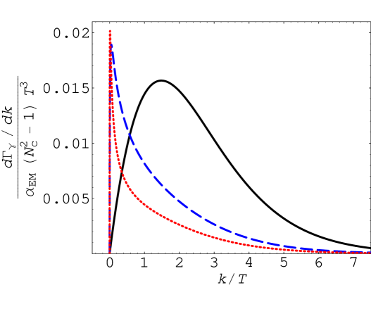
Figure 12: Photo-emission spectrum $d\Gamma_{\gamma}/dk$, divided by $\alpha_{\rm EM}(N_{\rm c}^{2}-1)T^{3}$, in $\mathcal{N}\,{=}\,4$ supersymmetric Yang-Mills theory for $\lambda=\infty$ (solid black curve), $\lambda=0.5$ (dashed blue), and $\lambda=0.2$ (dotted red). As explained in footnote 23, the weak-coupling curves interpolate between the rising small-frequency result (56), valid for $k\lesssim\lambda^{2}T$, and the falling large-frequency result (57), valid for $k\gg\lambda^{2}T$; the precise height of the sharp narrow peak is not known.

Fig. 12 illustrates how the photo-emission spectrum evolves as $\lambda$ increases. The slope at $k=0$ (proportional to the conductivity) decreases, the position and width of the hydrodynamic peak (both proportional to $\lambda^{2}T$) increase, and the amplitude of the spectrum for $k/T\mbox{~{}{\raisebox{1.72218pt}{$>$}} {\raisebox{-2.58334pt}{$\sim$}}~{}}1$ increases [due to the factor of $m_{\infty}^{2}\propto\lambda$ in Eq. (57)]. Figure 12 also shows the strong coupling result (58). The strong coupling curve differs primarily in having the temperature $T$, and not some smaller scale, set the width of the hydrodynamic regime (in which $d\Gamma_{\gamma}/dk$ is approximately linear in $k$). As a result, there is a broad maximum in the strong coupling spectrum at $k_{\rm max}\approx 1.5T$. At sufficiently small frequencies, the photon production rate is largest in the most weakly coupled theory. This is because, at these frequencies, the photon wavelength is larger than the free path of the particles involved, so the charges are effectively diffusing; weak coupling means faster diffusion and therefore more current on such long scales. The cross-over point, below which the weak-coupling rate exceeds the ($\lambda$ independent) strong-coupling rate, scales as $\lambda^{2/3}T$. At large frequency, the production rate is greatest in the strongly coupled theory. This is because the spectrum, for weak coupling, is proportional to the gauge coupling $\lambda\ll 1$ [appearing in Eq. (57) as the factor $m_{\infty}^{2}=\lambda T^{2}$], while the spectrum in the strong coupling limit has no such suppression. The results are clearly consistent with an expectation of smooth evolution between the weak and strong coupling regimes.

It is instructive to compare our weak-coupling result for $d\Gamma_{\gamma}/dk$ with the corresponding result for QCD AMY3 . But before this can be done in a meaningful fashion, we must first address the question of what normalization of the $U(1)$ current in SYM-EM will best mimic the electromagnetic physics of a real QGP. One can consider various different criteria for fixing the charge (or current) normalization in order to compare results between different theories. But for our purposes (involving the comparison of electromagnetic emission phenomena), the most natural criterion for fixing the normalization of the EM current in SYM-EM is to require that the dilepton emission spectra agree at large invariant mass. This amounts to demanding that the leading behavior of the current-current spectral density at large time-like momentum coincide in the two theories. This provides a simple criterion which will fix the normalization of the current, independent of the interaction strength in SYM, because all medium dependent corrections to the spectral density $\chi_{\mu}^{\mu}(K)$ vanish exponentially when $|K^{2}|\gg T^{2}$. Coinciding behavior of current-current spectral density at large timelike momenta also implies coinciding behavior at large spacelike momenta, and hence this criterion is the same as demanding that the leading short distance behavior of the $\langle J_{\mu}^{\rm EM}(x)J_{\nu}^{\rm EM}(0)\rangle$ correlator agree between theories. (Hence this criterion is the same as that used in Ref. wall3 .)

The particular choice of current we made in Eq. (8) happens to make the fermionic contribution to the large momentum behavior of the current-current spectral density the same as in QCD with three flavors (and $N_{\rm c}=3$). This merely reflects the fact that the sum of squares of the fermion charges coincide. But the scalars of $\mathcal{N}\,{=}\,4$ SYM contribute half as much as the fermions to the high momentum spectral density. Consequently, to satisfy the condition of coinciding large momentum behavior of the spectral density (for $N_{\rm f}=N_{\rm c}=3$), the $U(1)$ current used in our SYM calculations should be rescaled by a factor of $\sqrt{2/3}$. This we do in the following comparisons.

Once the normalization of the $U(1)$ current is fixed, the only other adjustable parameter in the SYM emission spectra is the value of the gauge (or ’t Hooft) coupling $\lambda$. If one compares photon emission in three-flavor QCD and $\mathcal{N}\,{=}\,4$ SYM, at $N_{\rm c}=3$ and the same value of the gauge coupling in both theories, then the SYM photo-emission rate is dramatically larger than the QCD rate, as shown in Fig. 13. This difference arises because the scattering rate in the SYM plasma is much higher than in QCD, owing to the larger number of matter fields and the fact that they are in the adjoint representation. In particular, the rate at which a quark undergoes photon producing Compton-type scattering is proportional to $m_{\infty}^{2}$, which is 9 times larger in SYM than in QCD (for equal values of the gauge coupling). The rate of Coulomb scattering, important in bremsstrahlung, is proportional to $m_{\rm D}^{2}$, which is 4 times larger.

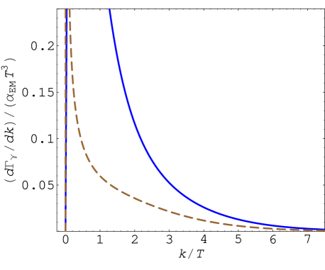
Figure 13: Comparison of leading-order photo-emission spectra for three-flavor massless QCD and $\mathcal{N}\,{=}\,4$ SYM (for $N_{\rm c}\,=3$), when the gauge coupling has the same value, $\alpha_{\rm s}=0.1$, in both theories. The upper solid curve shows the SYM result, while the lower dashed curve is the QCD result.

Because of this difference in scattering rates, it is more appropriate to compare the two theories with the SYM gauge coupling adjusted to give either the same value of the Debye mass $m_{\rm D}$ (in which case $\lambda^{\rm SYM}={\textstyle{\frac{1}{4}}}\lambda^{\rm QCD}$), or the same value of $m_{\infty}$ for the fermions as in QCD (in which case $\lambda^{\rm SYM}={\textstyle{\frac{1}{9}}}\lambda^{\rm QCD}$). Both of these comparisons are shown in Fig. 14. With coinciding values of the Debye mass, shown on the left of Fig. 14, the two spectra are nearly identical at high momenta, $k\gtrsim 3T$, while the SYM rate is larger at lower momenta (about 75% larger at $k/T=1$). When the two theories are compared at coinciding values of the asymptotic fermion mass $m_{\infty}$, as shown on the right hand plot of Fig. 14, the resulting curves are remarkably similar, with the SYM spectrum just a bit below the QCD result.

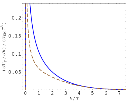
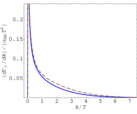
Figure 14: Comparison of leading-order photo-emission spectra for three-flavor massless QCD (dashed curve) and $\mathcal{N}\,{=}\,4$ SYM (solid curve) at $N_{\rm c}\,=3$. Left: equal values of the Debye mass $m_{\rm D}$ in both theories, corresponding to $\alpha_{\rm\scriptscriptstyle SYM}=0.025$ in SYM and $\alpha_{\rm s}=0.1$ in QCD. Right: equal values of the asymptotic fermion mass $m_{\infty}$, corresponding to $\alpha_{\rm\scriptscriptstyle SYM}=0.011$ in SYM and $\alpha_{\rm s}=0.1$ in QCD.

A major motivation of this work was the hope that one would be able to translate knowledge of the photon production rate in strongly coupled SYM into a useful prediction for the rate in strongly coupled QCD. This seems reasonably plausible given that (for comparable numbers of charged quarks) the weak coupling photon spectra of the two theories are quite similar, as shown in Fig. 14 — provided one scales the ’t Hooft coupling of SYM relative to that of QCD by a factor somewhere in the range 4–9. However, it is not clear if the quark-gluon plasma produced in heavy ion collisions can be well modeled by SYM plasma in the asymptotically strongly coupled $\lambda\to\infty$ limit. A comparison of Eq. (28) and Eq. (44) at, say, $k=5T$, shows that the weak coupling result approaches within 20% of the strong coupling result at $\lambda^{\rm SYM}\approx 4$. Taking this as a guess for the beginning of the region where the asymptotic strong coupling result provides a decent approximation, and applying the above rescaling between SYM and QCD gauge couplings yields $\alpha_{\rm s}^{\rm QCD}$ in the range 0.4–1.0, somewhat larger than the values of $\alpha_{\rm s}\approx 0.3$–0.5 commonly thought to be relevant in the QGP formed in heavy ion collisions. Therefore, it may be best to view the photon production rate in infinitely strongly-coupled SYM, for $k/T>1$, as an upper bound on what we expect the photon production rate from real QGP to be. Nevertheless, it will be interesting to see if incorporation of the strong coupling SYM spectral functions into models of photon production in heavy ion collisions improves the comparison with data. We have recently learned that efforts to do so are underway Jan-e .

Regarding dilepton emission, our results have a simple and more positive implication. Sufficiently deep in the timelike region, thermal corrections to the spectral function become very small for both weak and strong coupling. This is shown explicitly in Fig. 15, which plots the relative correction to the zero temperature spectral density as a function of $\sqrt{-K^{2}}$. If $|K^{2}|\geq(2\pi T)^{2}$, then thermal corrections to spectral function at weak coupling are under 2%. At strong coupling the corrections are larger, but nevertheless no more than 15% in this regime. Since the zero temperature spectral density is independent of coupling, as discussed in Section III, this means that the dilepton spectrum is nearly identical at weak and strong coupling, as long as the invariant mass of the pair is above $2\pi T$. This is also consistent with the modest size of the next-to-leading order weak-coupling result in QCD Majumder , which is a relative correction of $-{\textstyle{\frac{8}{9}}}(\alpha_{\rm s}/2\pi)(2\pi T)^{2}/K^{2}$. Therefore, for large invariant mass dilepton pairs, it is undoubtedly an excellent approximation to use the lowest-order production rate calculation even when the coupling is strong.

\psfrag{sqrtK2}{\raisebox{-4.30554pt}{\footnotesize$\sqrt{w^{2}-q^{2}}$}}\psfrag{SYM1}{\raisebox{4.30554pt}{SYM, $\lambda{=}0$}}\psfrag{SYM2}{\raisebox{4.30554pt}{SYM, $\lambda{=}\infty$}}\psfrag{delChimmrel}{$\Delta\chi^{\mu}_{\ \mu}/\chi^{\mu}_{\ \mu}(T{=}0)$}\includegraphics[width=252.94499pt]{deltaChirel-vs-K-weak.eps}

\psfrag{sqrtK2}{\raisebox{-4.30554pt}{\footnotesize$\sqrt{w^{2}-q^{2}}$}}\psfrag{SYM1}{\raisebox{4.30554pt}{SYM, $\lambda{=}0$}}\psfrag{SYM2}{\raisebox{4.30554pt}{SYM, $\lambda{=}\infty$}}\psfrag{delChimmrel}{$\Delta\chi^{\mu}_{\ \mu}/\chi^{\mu}_{\ \mu}(T{=}0)$}\includegraphics[width=252.94499pt]{deltaChirel-vs-K-strong.eps}

Figure 15: Relative size of the thermal corrections to the trace of the spectral function, $\Delta\chi^{\mu}_{\ \mu}(k^{0},k)$ divided by $\chi^{\mu}_{\ \mu}(k^{0},k)|_{T=0}$, as a function of $|K|/(2\pi T)=\sqrt{w^{2}-q^{2}}$ for $q\equiv k/(2\pi T)$ = 0 (black), 1 (blue), 2 (green), and 3 (red). The left panel shows the weak-coupling $\lambda\to 0$ result, while the right panel shows the strong coupling $\lambda\to\infty$ result.

Our results for photon and dilepton emission rates at strong coupling can be extended in a number of obvious ways. One question is how the emission spectra at strong coupling change if the field theory deviates from the conformally symmetric $\mathcal{N}\,{=}\,4$ SYM case. As discussed above, perturbative rates of photon production in conformal $\mathcal{N}\,{=}\,4$ SYM and in (non-conformal) QCD do not differ significantly, when compared at the same value of the thermal fermion mass. This suggests that the presence or absence of conformal symmetry does not play a decisive role in determining the perturbative photon spectrum. AdS/CFT can provide a similar comparison at strong coupling. For example, it should be possible to compute photon and dilepton emission spectra in both mass-deformed $\mathcal{N}\,{=}\,4$ SYM N=2* , and in $\mathcal{N}\,{=}\,4$ SYM at non-zero chemical potential, at strong coupling. A further question is related to the coupling constant dependence of the emission rates. It would be interesting to see how the spectrum shown in Fig. 12 evolves when $O(\lambda^{-3/2})$ corrections Buchel:2004di are taken into account. It would also be interesting to extend our analysis to theories with matter fields in the fundamental representation of the gauge group. Adding fundamental representation matter to $\mathcal{N}\,{=}\,4$ SYM corresponds, in the gravity dual, to the addition of D7 branes embedded in the $AdS_{5}\times S^{5}$ geometry KarchKatz . In such theories, it is natural to regard a flavor symmetry current of the fundamental matter fields as the electromagnetic current. Analyzing vector fluctuations on the $D7$ brane would then allow one to compute, at strong coupling, photon production from fundamental representation quarks of arbitrary mass added to the $\mathcal{N}\,{=}\,4$ SYM plasma.

Appendix A Asymptotics of the spectral function

For null momenta ($w{=}q$), Eq. (16a) for the transverse component of the electric field has the form

$$E_{\perp}^{\prime\prime}-\frac{2u}{f}\,E_{\perp}^{\prime}+\frac{w^{2}u}{f^{2}}\,E_{\perp}=0\,.$$ (60)

The solution obeying the incoming wave boundary condition at the horizon ($u=1$) is

$$E_{\perp}(u)=(1-u)^{-iw/2}(1+u)^{-w/2}\,{{}_{2\!}F_{1}}\!\left(-{\textstyle{\frac{1}{2}}}{(1{+}i)w}\,,1{-}{\textstyle{\frac{1}{2}}}{(1{+}i)w};1{-}iw;{\textstyle{\frac{1}{2}}}{(1-u)}\right)\,.$$ (61)

We are interested in asymptotics of the solution (61) for large and small values of $w$. To the best of our knowledge, appropriate asymptotic expansions of the hypergeometric function are unavailable in the literature. However, such expansions can be readily derived from the differential equation (60) following the approach of Ref. hep-th/0104065 .

For $w\gg 1$, we use the Langer-Olver method olver for constructing uniform asymptotic expansions (a version of the WKB approximation). Introducing new variables,

$$E_{\perp}(u)=\frac{1}{\sqrt{-f(u)}}\;y(u)\,,\qquad\qquad x=-u\,,$$ (62)

one can rewrite Eq. (60) as

$$y^{\prime\prime}(x)=\frac{w^{2}x-1}{(1-x^{2})^{2}}\;y(x)\,.$$ (63)

For $w\rightarrow\infty$, the dominant term on the right-hand side of Eq. (63) has a simple zero at $x=0$ and thus according to Ref. olver the asymptotics can be expressed in terms of Airy functions. Moreover, since the coefficients of Eq. (63) satisfy the conditions of Theorem 3.1 of Chapter XI in Ref. olver , one is guaranteed to have a uniform asymptotic expansion for all $u\in[0,1]$. The asymptotic expansion is

$$E_{\perp}(u)\sim\frac{C(w)}{\sqrt{-f(u)}}\;\hat{f}^{-1/4}(-u)\;\mbox{Ai}\left(w^{2/3}\zeta(-u)\right)+\cdots\,,$$ (64)

where $\mbox{Ai}(z)$ is the Airy function,

$$\zeta(x)\equiv\frac{3^{2/3}}{2^{4/3}}\left(i\pi-2\arctan{\sqrt{x}}+\log{\frac{\sqrt{x}+1}{\sqrt{x}-1}}\right)\,,\qquad\hat{f}(x)\equiv\frac{x}{(1-x^{2})^{2}\,\zeta(x)}\,,$$ (65)

and the ellipses denote corrections that can be systematically computed olver . The normalization constant,

$$C(w)=2\sqrt{\pi}e^{i\pi/4}\,w^{1/6}\,2^{-iw-w/2}\,e^{i\pi w/4}\,,$$ (66)

is chosen in such a way that the asymptotic expansion (64) coincides with the exact solution (61) as $u\rightarrow 1$, where $E_{\perp}\rightarrow(1{-}u)^{-iw/2}\,2^{-w/2}$. Using the asymptotic solution (64), for the retarded correlators we find

$$\Pi^{T}(w{=}q)\sim-\frac{N_{c}^{2}T^{2}}{8}\,\frac{(-w)^{2/3}\,3^{1/3}\,\Gamma(2/3)}{\Gamma(1/3)}\,,\qquad w\gg 1\,.$$ (67)

Correspondingly, for the trace of the spectral function we obtain

$$\chi^{\mu}_{\ \mu}(w{=}q)\sim\frac{N_{c}^{2}T^{2}\,w^{2/3}}{4}\,\frac{3^{5/6}\,\Gamma(2/3)}{\Gamma(1/3)}\,,\qquad w\gg 1\,.$$ (68)

In the low-frequency limit, one can solve Eq. (60) perturbatively using $w\ll 1$ as a small parameter. Since this procedure is well known (see, for example, Refs. hep-th/0104065 ; hep-th/0205052 ), we omit the details. The retarded correlator for $w\ll 1$ is given by

$$\Pi^{T}(w{=}q)=-{\textstyle{\frac{i}{8}}}{N_{c}^{2}T^{2}\,w}\left[1+iw\log{2}-{\textstyle{\frac{1}{12}}}{\pi^{2}}w^{2}+O(w^{3})\right],$$ (69)

and the resulting trace of the spectral function is

$$\chi^{\mu}_{\ \mu}(w{=}q)={\textstyle{\frac{1}{2}}}{N_{c}^{2}T^{2}\,w}\left[1-{\textstyle{\frac{1}{12}}}{\pi^{2}}\,w^{2}+O(w^{4})\right]\,.$$ (70)

References

- (1) For a review, see P. Stankus, Direct photon production in relativistic heavy-ion collisions, Ann. Rev. Nucl. Part. Sci. 55, 517 (2005).
- (2) S. S. Adler et al. [PHENIX Collaboration], Measurement of identified and inclusive photon and implication to the direct photon production in GeV Au+Au collisions, Phys. Rev. Lett. 96, 032302 (2006), nucl-ex/0508019;
- (3) S. S. Adler et al. [PHENIX Collaboration], Centrality dependence of direct photon production in GeV Au+Au collisions, Phys. Rev. Lett. 94, 232301 (2005), nucl-ex/0503003.
- (4) L. E. Gordon and W. Vogelsang, Polarized and unpolarized prompt photon production beyond the leading order, Phys. Rev. D 48, 3136 (1993).
- (5) P. Arnold, G. D. Moore and L. G. Yaffe, Photon emission from quark gluon plasma: Complete leading order results, JHEP 0112, 009 (2001), hep-ph/0111107.
- (6) See, for example M. Le Bellac, Thermal Field Theory, Cambridge, 1996.
- (7) P. Aurenche, F. Gelis, G. D. Moore and H. Zaraket, Landau-Pomeranchuk-Migdal resummation for dilepton production, JHEP 0212, 006 (2002), hep-ph/0211036.
- (8) F. Karsch, E. Laermann, P. Petreczky, S. Stickan and I. Wetzorke, A lattice calculation of thermal dilepton rates, Phys. Lett. B 530, 147 (2002), hep-lat/0110208.
- (9) S. Gupta, The electrical conductivity and soft photon emissivity of the QCD plasma, Phys. Lett. B 597, 57 (2004), hep-lat/0301006.
- (10) G. Aarts, C. Allton, J. Foley, S. Hands and S. Kim, Meson spectral functions at nonzero momentum in hot QCD, hep-lat/0607012.
- (11) J. P. Blaizot and F. Gelis, Photon and dilepton production in the quark-gluon plasma: Perturbation theory vs lattice QCD, Eur. Phys. J. C 43, 375 (2005), hep-ph/0504144.
- (12) For a review, see O. Aharony, S. S. Gubser, J. M. Maldacena, H. Ooguri and Y. Oz, Large field theories, string theory and gravity, Phys. Rept. 323, 183 (2000), hep-th/9905111.
- (13) P. Kovtun and A. Starinets, Thermal spectral functions of strongly coupled supersymmetric Yang-Mills theory, Phys. Rev. Lett. 96, 131601 (2006), hep-th/0602059.
- (14) D. Teaney, Finite temperature spectral densities of momentum and -charge correlators in Yang Mills theory, Phys. Rev. D 74, 045025 (2006) hep-ph/0602044.
- (15) D. T. Son and A. O. Starinets, Minkowski-space correlators in AdS/CFT correspondence: Recipe and applications, JHEP 0209, 042 (2002), hep-th/0205051.
- (16) G. Policastro, D. T. Son and A. O. Starinets, From AdS/CFT correspondence to hydrodynamics, JHEP 0209, 043 (2002), hep-th/0205052.
- (17) A. Nunez and A. O. Starinets, AdS/CFT correspondence, quasinormal modes, and thermal correlators in SYM, Phys. Rev. D 67, 124013 (2003), hep-th/0302026.
- (18) P. K. Kovtun and A. O. Starinets, Quasinormal modes and holography, Phys. Rev. D 72, 086009 (2005), hep-th/0506184.
- (19) D. Anselmi, D. Z. Freedman, M. T. Grisaru and A. A. Johansen, Nonperturbative formulas for central functions of supersymmetric gauge theories, Nucl. Phys. B 526, 543 (1998), hep-th/9708042.
- (20) See, for example, C. M. Bender, S. A. Orszag, Advanced Mathematical Methods for Scientists and Engineers, Springer, 1999.
- (21) See, for example, Eq. (15.3.4) of M. Abramowitz and I. A. Stegun, Ed., Handbook of Mathematical Functions, Dover, New York, 1970.
- (22) T. Umeda, K. Nomura and H. Matsufuru, Charmonium at finite temperature in quenched lattice QCD, Eur. Phys. J. C 39S1, 9 (2005), hep-lat/0211003.
- (23) M. Asakawa and T. Hatsuda, and in the deconfined plasma from lattice QCD, Phys. Rev. Lett. 92, 012001 (2004), hep-lat/0308034.
- (24) S. Datta, F. Karsch, P. Petreczky and I. Wetzorke, Behavior of charmonium systems after deconfinement, Phys. Rev. D 69, 094507 (2004), hep-lat/0312037.
- (25) A. Jakovac, P. Petreczky, K. Petrov and A. Velytsky, On charmonia survival above deconfinement, hep-lat/0603005.
- (26) E. V. Shuryak and I. Zahed, Rethinking the properties of the quark gluon plasma at , Phys. Rev. C 70, 021901 (2004), hep-ph/0307267.
- (27) E. Witten, Anti-de Sitter space, thermal phase transition, and confinement in gauge theories, Adv. Theor. Math. Phys. 2, 505 (1998), hep-th/9803131.
- (28) For an introduction, see J. M. Maldacena, TASI-2003 lectures on AdS/CFT, hep-th/0309246.
- (29) For a phenomenological application, see J. Erlich, E. Katz, D. T. Son and M. A. Stephanov, QCD and a holographic model of hadrons, Phys. Rev. Lett. 95, 261602 (2005), hep-ph/0501128.
- (30) C. P. Herzog, A holographic prediction of the deconfinement temperature, hep-th/0608151.
- (31) P. Arnold, G. D. Moore and L. G. Yaffe, Photon emission from ultrarelativistic plasmas, JHEP 0111, 057 (2001), hep-ph/0109064.
- (32) R. Baier, H. Nakkagawa, A. Niegawa and K. Redlich, Production rate of hard thermal photons and screening of quark mass singularity, Z. Phys. C 53, 433 (1992).
- (33) J. I. Kapusta, P. Lichard and D. Seibert, High-energy photons from quark-gluon plasma versus hot hadronic gas, Phys. Rev. D 44, 2774 (1991) [Erratum-ibid. D 47, 4171 (1993)].
- (34) P. Aurenche, F. Gelis, R. Kobes and H. Zaraket, Bremsstrahlung and photon production in thermal QCD, Phys. Rev. D 58, 085003 (1998), hep-ph/9804224.
- (35) L. D. Landau and I. Pomeranchuk, Limits of applicability of the theory of bremsstrahlung electrons and pair production at high-energies, Dokl. Akad. Nauk Ser. Fiz. 92, 535 (1953).
- (36) A. B. Migdal, Quantum kinetic equation for multiple scattering, Dokl. Akad. Nauk Ser. Fiz. 105, 77 (1955).
- (37) A. B. Migdal, Bremsstrahlung and pair production in condensed media at high-energies, Phys. Rev. 103, 1811 (1956).
- (38) E. Braaten and R. D. Pisarski, Soft amplitudes in hot gauge theories: A general analysis, Nucl. Phys. B 337, 569 (1990).
- (39) P. Aurenche, F. Gelis and H. Zaraket, A simple sum rule for the thermal gluon spectral function and applications, JHEP 0205, 043 (2002), hep-ph/0204146.
- (40) G. D. Moore and J. M. Robert, Dileptons, spectral weights, and conductivity in the quark-gluon plasma, hep-ph/0607172.
- (41) P. Arnold, G. D. Moore and L. G. Yaffe, Transport coefficients in high temperature gauge theories. I: Leading-log results, JHEP 0011, 001 (2000), hep-ph/0010177.
- (42) P. Arnold, G. D. Moore and L. G. Yaffe, Transport coefficients in high temperature gauge theories. II: Beyond leading log, JHEP 0305, 051 (2003), hep-ph/0302165.
- (43) Jan-e Alam, private communication.
- (44) A. Majumder and C. Gale, On the imaginary parts and infrared divergences of two-loop vector boson self-energies in thermal QCD, Phys. Rev. C 65, 055203 (2002), hep-ph/0111181.
- (45) A. Buchel and J. T. Liu, Thermodynamics of the * flow, JHEP 0311, 031 (2003), hep-th/ 0305064.
- (46) A. Buchel, J. T. Liu and A. O. Starinets, Coupling constant dependence of the shear viscosity in supersymmetric Yang-Mills theory, Nucl. Phys. B 707, 56 (2005) hep-th/0406264.
- (47) A. Karch and E. Katz, Adding flavor to AdS/CFT, JHEP 0206, 043 (2002) hep-th/0205236.
- (48) G. Policastro and A. Starinets, On the absorption by near-extremal black branes, Nucl. Phys. B 610, 117 (2001), hep-th/0104065.
- (49) F. W. J. Olver, Asymptotics and special functions, A K Peters, Wellesley, 1997.