Bethe Ansatz solutions for highest states in ${\cal N}=4$ SYM and AdS/CFT duality

Abstract:

We consider the operators with highest anomalous dimension $\Delta$ in the compact rank-one sectors $\mathfrak{su}(1|1)$ and $\mathfrak{su}(2)$ of ${\cal N}=4$ super Yang-Mills. We study the flow of $\Delta$ from weak to strong ’t Hooft coupling $\lambda$ by solving (i) the all-loop gauge Bethe Ansatz, (ii) the quantum string Bethe Ansatz. The two calculations are carefully compared in the strong coupling limit and exhibit different exponents $\nu$ in the leading order expansion $\Delta\sim\lambda^{\nu}$. We find $\nu=1/2$ and $\nu=1/4$ for the gauge or string solution. This strong coupling discrepancy is not unexpected, and it provides an explicit example where the gauge Bethe Ansatz solution cannot be trusted at large $\lambda$. Instead, the string solution perfectly reproduces the Gubser-Klebanov-Polyakov law $\Delta=2\sqrt{n}\,\lambda^{1/4}$. In particular, we provide an analytic expression for the integer level $n$ as a function of the U(1) charge in both sectors.

1 Introduction

The AdS/CFT correspondence [1, 2, 3, 4, 5] is a non-trivial map between two integrable theories, string theory on $AdS_{5}\times S^{5}$ and the maximally supersymmetric ${\cal N}=4$ super Yang-Mills SU(N) gauge theory (SYM). In the planar limit $N\to\infty$, the string coupling vanishes and the correspondence relates a finite superconformal four dimensional theory and free string theory on a non-trivial background. Massive string states are predicted to be dual to certain composite operators in the gauge theory, with the string spectrum matching the gauge anomalous dimensions. In terms of the planar ’t Hooft coupling $\lambda=g^{2}_{\rm YM}\,N$, the duality is of the weak-strong coupling type. Hence, any test of the correspondence must exploit some kind of non-perturbative knowledge on at least one of the two sides.

The large $\lambda$ limit is particularly interesting since the string side can be controlled in the supergravity approximation. A quite general prediction is the scaling $E\sim 2\,\sqrt{n}\,\lambda^{1/4}$ for the energy of level $n$ massive string states as $\lambda\to\infty$ [2]. In the gauge theory, a check of this prediction requires the knowledge of the anomalous dimensions of suitable dual composite operators in the nonperturbative regime. Such a formidable task is made possible by the integrability properties of ${\cal N}=4$ SYM. The scaling operators are eigenstates of the dilatation operator $\mathfrak{D}$ that can be identified with the Hamiltonian of integrable (super) spin chains in various sectors closed under perturbative renormalization. The integrable operator $\mathfrak{D}$ can be treated by Bethe Ansatz techniques [6, 7, 8]. In particular, all-loop conjectured gauge Bethe Ansatz (GBA) equations are available in the compact $\mathfrak{su}(2)$, $\mathfrak{su}(1|1)$ and non-compact $\mathfrak{sl}(2)$ sectors [9, 10].

Unfortunately, the GBA equations are only asymptotically exact. For operators with classical dimension $L$, they predict the exact anomalous dimension up to wrapping terms appearing at a certain order increasing with $L$, for instance terms ${\cal O}(\lambda^{L})$ in the $\mathfrak{su}(2)$ sector [11]. Due to wrapping terms, the GBA equations are not reliable at strong coupling, although in some cases they are believed to give the correct leading term. Remarkably, in the $\mathfrak{su}(2)$ sector, a local version of the GBA equations has been proposed in the form of a Hubbard-like model [12]; it has been conjectured to be free from wrapping problems, but the reconciliation of its strong coupling predictions with string theory is far from clear [12, 13, 14].

In general, the gauge and string calculations overlap in BMN-like limits [15] where $L$ is large. In this case, it is well known that the perturbative comparison in powers of $\lambda$ is plagued by the different order of the limits $\lambda\to 0$, $L\to\infty$ on the two sides. For instance, the exact three-loop anomalous dimension of two- and three-magnon operators in the near-BMN limit [15] exhibits a three-loop discrepancy when compared with the leading curvature correction computed in string theory [16, 17, 18, 19]. Similar three-loop discrepancies also occur in the expansion around spinning string solutions [20, 11].

Along a different route, one can start from the classical string theory (at large $\lambda$) and derive thermodynamical Bethe Ansatz equations at $L\to\infty$. The discretization of these string Bethe Ansatz equations (SBA) have been proposed to compute the leading $1/L$ effects, i.e. one-loop worldsheet quantum corrections [21, 9, 10]. The validity of the SBA equations at finite $L$ or small $\lambda$ is not guaranteed and indeed they are known to receive several kinds of corrections [22, 23, 24, 25]. These corrections have been evaluated for various classes of Frolov-Tseytlin spinning string solutions [26, 27, 28, 29, 30, 31, 32]. They suggest the emergence of an interpolating set of Bethe Ansatz equations working at all $\lambda$ and $L$ [33, 34] and hopefully solving the three-loop discrepancies.

In this paper, we take a complementary approach by comparing the GBA and SBA equations at strong coupling. Indeed, it is not totally clear to what extent the GBA equations are able to predict the correct results in the string regime $\lambda\to\infty$ as discussed for instance in [13, 14, 35]. We attempt to answer this question for the states with highest anomalous dimension in the two compact rank-one $\mathfrak{su}(2)$ and $\mathfrak{su}(1|1)$ subsectors where we are able to solve the GBA and SBA equations at fixed $L$ and generic $\lambda$. To appreciate the special role of the highest states, we briefly summarize some relevant facts about them.

In the $\mathfrak{su}(2)$ sector, the highest state is the so-called antiferromagnetic (AF) operator [36]. It can be defined in the multiplet of operators with fixed classical dimension $L$. At the perturbative level, it mixes with the other states and its explicit expression is not available in closed form at finite $L$. In the $L\to\infty$ limit, the GBA equations can be solved and give the anomalous dimension

$$\lim_{L\to\infty}\frac{\Delta_{\mathfrak{su}(2)}}{L}=1+\frac{\sqrt{\lambda}}{\pi}\int_{0}^{\infty}\frac{ds}{s}\,\,\frac{J_{0}\left(\frac{\sqrt{\lambda}}{2\pi}s\right)J_{1}\left(\frac{\sqrt{\lambda}}{2\pi}s\right)}{\,{\rm e}\,^{s}+1}\ .$$ (1)

This expression is obtained by taking the $L\to\infty$ limit at fixed $\lambda$. Hence, it is legitimate to expand at weak coupling and one obtains

$$\lim_{L\to\infty}\frac{\Delta_{\mathfrak{su}(2)}}{L}=1+4\ln 2\,\frac{\lambda}{16\pi^{2}}-9\,\zeta(3)\left(\frac{\lambda}{16\pi^{2}}\right)^{2}+75\,\zeta(5)\left(\frac{\lambda}{16\pi^{2}}\right)^{3}+\dots.$$ (2)

On the other hand, the strong coupling expansion of Eq. (1) is

$$\lim_{L\to\infty}\frac{\Delta_{\mathfrak{su}(2)}}{L}=\frac{1}{\pi^{2}}\,\sqrt{\lambda}+\frac{3}{4}+\dots.$$ (3)

The same leading term is obtained in the Hubbard model formulation of the GBA equations [13, 14]. As discussed in [36] this expansion is formal due to the uncontrolled effect of wrapping terms. The usual attitude toward this problem is rather optimistic and Eq.(3) with its $\sim\lambda^{1/2}$ signature is expected to be correct apart from a possible correction in the numerical prefactor $1/\pi^{2}$. As a support to the this scenario, it has been proposed to identify its dual string state with a suitable string solution in the spirit of similar correspondences found in the lowest part of the spectrum [37]. The slow-string solution described in [38] exhibits the $\lambda^{1/2}$ scaling of Eq. (3) although with a different numerical prefactor. This quantitative discrepancy has been attributed in [38] to the subtle double limit $\lambda,L\to\infty$. However, the Hubbard model formulation [12] suggests that this scenario is not entirely satisfactory. There, limit ambiguities and wrapping problems are absent and nevertheless the same prediction $\Delta/L\sim\sqrt{\lambda}/\pi^{2}$ is recovered including the prefactor [13, 14]. A more convincing proof should at least include the analysis of the solution of the SBA equations, valid in the strong coupling limit.

A similar analysis can be attempted for the highest operator in the other compact sector $\mathfrak{su}(1|1)$ [35]. Here the precise form of the operator is known at finite $L$ and simply reads $\mbox{Tr}(\psi^{L})$ where $\psi$ is the highest weight component of the Weyl spinor in the vector multiplet. Unfortunately, a closed formula like Eq. (1) is not known in this sector. In [35], the GBA equations for the highest state are studied at weak and strong coupling in the $L\to\infty$ limit. The weak coupling expansion turns out to have a finite but rather small convergence radius and is not immediately useful to reach the strong coupling regime. On the other hand, the strong coupling expansion is ambiguous and depends on assumptions about the large $\lambda$ behavior of the Bethe parameters [21]. Two asymptotic solutions for the Bethe momenta have been proposed in [35]. The leading term in the anomalous dimension is the same in both cases and scales like $\lambda^{1/2}$.

To summarize, the present knowledge on the strong coupling behavior of the maximal states in the compact sectors of ${\cal N}=4$ SYM is (we write only the leading term at large $\lambda$ and define $L$ to be the number of Bethe momenta in both sectors)

$$\begin{array}[]{ccll}\displaystyle\lim_{L\to\infty}\frac{\Delta_{\mathfrak{su}(2)}^{\rm gauge}}{2L}&=&\displaystyle\frac{1}{\pi^{2}}\,\lambda^{1/2},&(\mbox{exact})\\ \\ \displaystyle\frac{\Delta_{\mathfrak{su}(1|1)}^{\rm gauge}}{L}&=&\displaystyle c_{L}\,\lambda^{1/2},&(\mbox{conjecture}\,\cite[cite]{[\@@bibref{}{Arutyunov:2006av}{}{}]})\end{array}\qquad\begin{array}[]{ccl}\displaystyle\lim_{L\to\infty}\frac{\Delta_{\mathfrak{su}(2)}^{\rm string}}{2L}&=&\mbox{?},\\ \\ \displaystyle\lim_{L\to\infty}\frac{\Delta_{\mathfrak{su}(1|1)}^{\rm string}}{L}&=&\mbox{?},\end{array}$$ (4)

$$c_{L}\to\displaystyle\frac{3\sqrt{3}}{2\pi^{2}},\quad\mbox{as}\ L\to\infty,$$

where the superscripts gauge/string label the results obtained with the GBA/SBA equations.

In this paper, we pursue the analysis of these states with the aim of filling the gaps in the above predictions. We begin with the $\mathfrak{su}(1|1)$ sector which is particularly favorable from the technical point of view. At weak coupling we present high-order results for the anomalous dimension computed by the GBA equations. We show that a resummation is possible by a non-linear acceleration method, the Weniger algorithm. It permits to evaluate the anomalous dimension for rather large values of the coupling $\lambda$. This leads to results supporting the $\lambda^{1/2}$ asymptotic behavior, although with a different coefficient with respect to the proposals in [35].

To investigate further the flow from weak to strong coupling we present a numerical solution of the GBA equations. It is worthwile to emphasize that the analysis is quite robust and can be extended to very large values of $\lambda$ following in a clean way the evolution of Bethe momenta. Our analysis reveals several subtleties involved in the strong coupling expansion of the GBA equations. The final result is simple and we are able to compute very precisely the leading strong-coupling term of the anomalous dimension. Not suprisingly, the agreement with the weak coupling resummation is quite good. At this point, the information about the highest state is similar to what is known in the $\mathfrak{su}(2)$ sector. We have accurately computed the weak coupling expansion and the leading asymptotic $\lambda^{1/2}$ term, but we do not know to what extent the GBA are reliable in the strong coupling region. We remark that, in the $\mathfrak{su}(1|1)$ sector, we do not have a slow-string limit solution to be identified with the highest state.

The next obvious step is to analyze the SBA equations in this sector by the same methods. Once again the string Bethe Ansatz equations can be integrated numerically. The result is very interesting. All Bethe momenta flow to zero at large $\lambda$ with a simple leading term $p_{k}\sim\alpha_{k}\,\lambda^{-1/4}$, and the asymptotic coefficients $\alpha_{k}$ can be computed numerically. We also determine analytically the prefactor in the leading term $\sim\lambda^{1/4}$ in the anomalous dimension.

The same analysis can be applied to the $\mathfrak{su}(2)$ sector. The weak coupling resummation does not apply here because the precise form of the highest AF state depends on $L$. However, the numerical and analytical study of the strong-coupling behavior of GBA and SBA equations can be performed without difficulty. We find a pattern similar to the $\mathfrak{su}(1|1)$ one. Our results are summarized in the following table which has to be compared with Eqs. (4). In the right hand sides, we only report the leading term at large $\lambda$ and finite $L$

$$\begin{array}[]{ccl}\displaystyle\frac{\Delta_{\mathfrak{su}(2)}^{\rm gauge}}{2L}&=&\displaystyle\frac{1}{2\pi L\sin{\displaystyle\frac{\pi}{2L}}}\,\lambda^{1/2},\\ \\ \displaystyle\frac{\Delta_{\mathfrak{su}(1|1)}^{\rm gauge}}{L}&=&\displaystyle c_{L}\,\lambda^{1/2},\end{array}\qquad\begin{array}[]{ccl}\displaystyle\frac{\Delta_{\mathfrak{su}(2)}^{\rm string}}{2L}&=&\displaystyle\frac{1}{2}\,\lambda^{1/4},\\ \\ \displaystyle\frac{\Delta_{\mathfrak{su}(1|1)}^{\rm string}}{L}&=&\displaystyle\frac{1}{\sqrt{2}}\left(1-\frac{1}{L^{2}}\right)\,\lambda^{1/4},\end{array}$$ (5)

$$c_{L}\to 0.1405(1),\quad\mbox{as}\ L\to\infty.$$

The ratio $\Delta_{\mathfrak{su}(2)}^{\rm string}/(2L)$ is independent on $L$. Also, in the $L\to\infty$ limit, we recover the exact prefactor $1/\pi^{2}$ for $\Delta_{\mathfrak{su}(2)}^{\rm gauge}/(2L)$.

The physical contents of Eqs. (5) will be discussed in Sec. 6, after heving illustrated the technical details of the derivation. These will be organized as follows. In Sec. 2, we present the gauge Bethe Ansatz equations for the $\mathfrak{su}(1|1)$ sector. In Sec. 2.1 and 2.2 we analyze them for the highest state obtaining in particular the strong coupling expansion of the anomalous dimension. Sec. 3 presents the string Bethe Ansatz equations, again for the $\mathfrak{su}(1|1)$ sector and Sec. 3.1 and 3.2 repeat the previous analysis. In this case, the strong coupling expansion of the anomalous dimension is determined exactly. In Sec. 4 and 5 we present a similar analysis for the other compact $\mathfrak{su}(2)$ sector.

2 The gauge Bethe Ansatz equations for the highest state in the $\mathfrak{su}(1|1)$ sector

The dilatation operator in the $\mathfrak{su}(1|1)$ sector can be associated with a super spin chain [39, 19]. The all-loop gauge Bethe Ansatz equations have been proposed in [9, 10] and read

$$e^{i\,L\,p_{k}}=\prod_{j\neq k}\frac{\displaystyle 1-\frac{g^{2}}{2\,x^{+}(p_{k})\,x^{-}(p_{j})}}{\displaystyle 1-\frac{g^{2}}{2\,x^{-}(p_{k})\,x^{+}(p_{j})}},\qquad k=1,\dots,L,$$ (6)

where $L\in 2\mathbb{N}+1$ and

$$x^{\pm}(p)=\frac{e^{\pm i\,\frac{p}{2}}}{4\sin\frac{p}{2}}\left(1+\sqrt{1+8\,g^{2}\,\sin^{2}\frac{p}{2}}\right).$$ (7)

The coupling $g$ is related to the ’t Hooft coupling by $\lambda=8\,\pi^{2}\,g^{2}$. The anomalous dimension of the state associated with the solution $\{p_{k}(g^{2})\}$ is

$$\Delta=\frac{3}{2}\,L+\sum_{k=1}^{L}\left(\sqrt{1+8\,g^{2}\,\sin^{2}\frac{p_{k}}{2}}-1\right).$$ (8)

The Bethe momenta of the highest state at $g=0$ are

$$p_{k}=\frac{2\pi}{L}\,n_{k},\qquad n_{k}=-\frac{L-1}{2},\dots,\frac{L-1}{2}.$$ (9)

The GBA equations in logarithmic forms are

$$p_{k}=\frac{2\pi}{L}\,n_{k}-\frac{i}{L}\sum_{j\neq k}\log\frac{\displaystyle 1-\frac{g^{2}}{2\,x^{+}_{k}\,x^{-}_{j}}}{\displaystyle 1-\frac{g^{2}}{2\,x^{-}_{k}\,x^{+}_{j}}},$$ (10)

where $n_{k}$ are given in (9). They are suitable for weak coupling expansions since the second term in the r.h.s. is ${\cal O}(g^{2})$.

2.1 Weak coupling expansion and Weniger resummation

The weak-coupling expansion of the anomalous dimension is easily obtained. We simply start with the zero-th order value of Bethe momenta for a certain fixed $L$, Eq. (9). Then, we replace them in the GBA equation and expand the r.h.s. at first order in $g^{2}$. Repeating this procedure and expanding the expression for $\Delta$ order by order, we obtain the perturbative expansion of $\Delta$.

In the ratio $\Delta/L$, the terms up to ${\cal O}(g^{2L-2})$ do not change if $L$ is increased. For instance,

$$\left(\frac{\Delta}{L}\right)_{L=3} = \frac{3}{2}+2\,g^{2}-4\,g^{4}+14\,g^{6}-\frac{235}{4}\,g^{8}+\frac{2209}{8}\,g^{10}+\cdots,$$ (11)

$$\left(\frac{\Delta}{L}\right)_{L=5} = \frac{3}{2}+2\,g^{2}-4\,g^{4}+\frac{29}{2}\,g^{6}-\frac{259}{4}\,g^{8}+\frac{2611}{8}\,g^{10}+\cdots,$$ (12)

$$\left(\frac{\Delta}{L}\right)_{L=7} = \frac{3}{2}+2\,g^{2}-4\,g^{4}+\frac{29}{2}\,g^{6}-\frac{259}{4}\,g^{8}+\frac{1307}{4}\,g^{10}+\cdots,$$ (13)

This remark allows one to compute the $L\to\infty$ limit of the expansion at a fixed order in $g$ by simply taking a sufficiently large $L$. The procedure can be performed at the semi-numerical level. In other words, we work with finite high precision using numerical values of the momenta in a symbolic algebra calculation. If the precision is suitably high, the identification of the coefficients of the energy expansion can be unambiguously identified with rational numbers. We have performed the calculation up to the term $g^{68}$. This requires $L\geq 35$. The result is

$$\lim_{L\to\infty}\frac{\Delta}{L} = \textstyle\frac{3}{2}+2\,g^{2}-4\,g^{4}+\frac{29}{2}\,g^{6}-\frac{259}{4}\,g^{8}+\frac{1307}{4}\,g^{10}-1790\,g^{12}+10396\,g^{14}-\frac{504397}{8}\,g^{16}$$ (14)

$$\textstyle+\frac{6324557}{16}\,g^{18}-\frac{40702709}{16}\,g^{20}+\frac{8561442701}{512}\,g^{22}-\frac{114529021311}{1024}\,g^{24}$$

$$\textstyle+\frac{777307887947}{1024}\,g^{26}-\frac{2670717561365}{512}\,g^{28}+\frac{37098574647961}{1024}\,g^{30}-\frac{4161069724993527}{16384}\,g^{32}$$

$$\textstyle+\frac{29408079892945107}{16384}\,g^{34}-\frac{104670245742870895}{8192}\,g^{36}+\frac{5999052730939686071}{65536}\,g^{38}$$

$$\textstyle-\frac{86452214868942845981}{131072}\,g^{40}+\frac{626162974135003430373}{131072}\,g^{42}-\frac{4556537471418865642837}{131072}\,g^{44}$$

$$\textstyle+\frac{66598702591887298874029}{262144}\,g^{46}-\frac{244303906058015917431755}{131072}\,g^{48}$$

$$\textstyle+\frac{7195137546781961772111605}{524288}\,g^{50}-\frac{106303776929607820974312023}{1048576}\,g^{52}$$

$$\textstyle+\frac{49230031886653815687152661}{65536}\,g^{54}-\frac{45726319914455572899079305}{8192}\,g^{56}$$

$$\textstyle+\frac{348843198908576206971428650203}{8388608}\,g^{58}-\frac{2605279742772089252587976183821}{8388608}\,g^{60}$$

$$\textstyle+\frac{39003030225010830621366145740085}{16777216}\,g^{62}-\frac{2340608578131628813286501122058923}{134217728}\,g^{64}$$

$$\textstyle+\frac{35185861176795745832756768610959237}{268435456}\,g^{66}$$

$$\textstyle-\frac{264968465576189708105542064159612145}{268435456}\,g^{68}+{\cal O}(g^{70}).$$

We have identified the rational numbers by working with 200 digits arithmetics . This power series is convergent for $g^{2}\lesssim\frac{1}{8}$, a rather small convergence radius. It is definitely useless to evaluate strong coupling behavior at least in this form. We need an analytical continuation beyond the convergence radius. Since the series is alternating, we have attempted such continuation by means of the non-linear Weniger algorithm [41] that we describe in Appendix A.

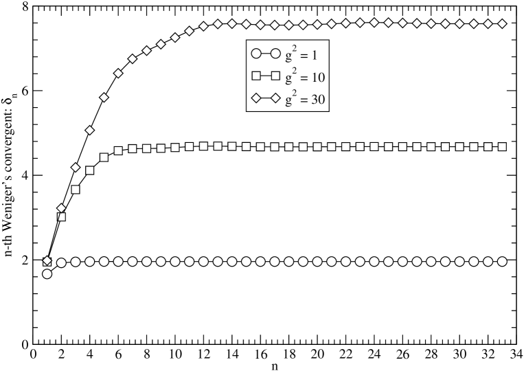
Figure 1: Weniger convergents $\delta_{n}(g^{2})$ for the weak coupling expansion of the GBA equations at the three values $g^{2}=1,10,30$.

In our case, the Weniger algorithm is found to work very well. As an example, we consider $g^{2}=1$ which is far beyond the convergence radius. The Weniger approximants are shown in the first curve of Fig. (1) where a clear and definite convergence is achieved. Going to higher values of the coupling, we find that the resummation algorithm gives stable results up to $g^{2}\simeq 20$, which is a fairly high value. The other two curves of Fig. (1) shows the behavior of Weniger approximants for $g^{2}=10,30$.

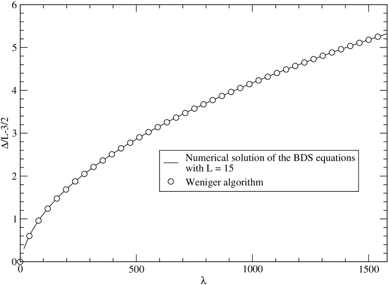
Figure 2: Resummation of the weak coupling expansion of the GBA equations. We also show the result from the iterative numerical solution of the same equations at $L=15$.

The plot of $\Delta/L-3/2$ at $L\to\infty$ in the stability region is shown in Fig. (2) where we also draw the results from the numerical analysis of the GBA equations that are discussed in the next Section. From the Weniger algorithm, we recover clearly the asymptotic $\sqrt{\lambda}$ behavior. A numerical fit gives the estimate

$$\lim_{L\to\infty}\frac{\Delta}{L}\sim 0.1404\,\sqrt{\lambda}.$$ (16)

The numerical prefactor is different than the one predicted in [35]. The question is whether the resummation is failing or the strong coupling expansion is revealing some surprise. In the next Section, we shall answer this question in favor of the second hypothesis.

2.2 Numerical solution and strong coupling behavior

2.2.1 Preliminary remarks

The form of the GBA equations at strong coupling depends crucially on certain a priori assumptions about the asymptotic form of Bethe momenta. For the highest state, it is necessary to consider separately three different cases, motivated by the following numerical analysis. If we denote by $p(g)$ a particular running Bethe momentum, we consider the three special large-$g$ behaviors

I $$: p(g)\to\overline{p}>0,$$

II $$: p(g)\sim\alpha\,g^{-1/2},$$ (17)

III $$: p(g)\sim\alpha\,g^{-1}.$$

The ratio $g/x^{\pm}(p)$ has the following limit

$$\frac{g}{x^{\pm}(p)}\to\left\{\begin{array}[]{ll}\mbox{I:}&\sqrt{2}\,e^{\mp i\frac{\overline{p}}{2}}\,\varepsilon(\sin\frac{\overline{p}}{2}),\\ \\ \mbox{II:}&\sqrt{2}\,\varepsilon(\alpha),\\ \\ \mbox{III:}&\displaystyle\frac{2\alpha}{1+\sqrt{1+2\alpha^{2}}},\end{array}\right.$$ (18)

where $\varepsilon(x)=x/|x|$ is the sign function. For better uniformity, it is convenient to write the case II as

$$\sqrt{2}\,\varepsilon(\alpha)\equiv\sqrt{2}\,e^{\mp i\frac{\overline{p}}{2}}\,\varepsilon(\sin\frac{\overline{p}}{2}),$$ (19)

where $\overline{p}=0$ in this case, and $\varepsilon(0)=\pm 1$ according to the sign of $\alpha$. With these conventions, cases I and II are expressed by the same formula.

2.2.2 The Arutyunov-Tseytlin Ansatz

An Ansatz for the strong coupling behavior of the Bethe momenta of the highest state is described in [35]. As we shall discuss, it is closely related to the actual solution. The Arutyunov-Tseytlin Ansatz assumes that one $p$ remains zero and the other tend to non-zero limits symmetrically distributed around zero. This Ansatz is quite reasonable since the symmetric pattern is valid at $g=0$ and remains true at all orders in the weak coupling expansion.

Under this assumption, we can look at the positive $p$ only. Using the expressions (18), the GBA equation for any of them reduces at strong coupling to

$$e^{iLp_{k}}=e^{-ip_{k}}\,\mathop{\prod_{j=1}^{\frac{L-1}{2}}}_{j\neq k}\frac{1-e^{-\frac{i}{2}(p_{k}-p_{j})}}{1-e^{\frac{i}{2}(p_{k}-p_{j})}}\,\frac{1+e^{-\frac{i}{2}(p_{k}+p_{j})}}{1+e^{\frac{i}{2}(p_{k}+p_{j})}}=-\prod_{j=1}^{\frac{L-1}{2}}(-e^{-ip_{k}})$$ (20)

This gives

$$Lp_{k}=\frac{L-3}{2}\pi-\frac{L-1}{2}p_{k}+2\pi m_{k},\qquad m_{k}\in\mathbb{Z},$$ (21)

or

$$p_{k}=\frac{4\pi\,m_{k}}{3L-1}+\pi\frac{L-3}{3L-1}.$$ (22)

2.2.3 Explicit results at various $L$

As we discussed, the result (22) implies an asymptotic anomalous dimension which does not agree with the resummation results. To understand what is happening, we have solved numerically the gauge Bethe Ansatz equations according to the following recipe

1. we start with the solution at $g=0$,

2. we progressively increase $g$ and solve step by step the Bethe equations by Newton’s algorithm [42],

3. at each step, we use the solution at the previous $g$ as a starting guess for Newton’s algorithm.

The procedure turns out to be very stable and can be extended up to very large $\lambda$ values. In particular it is possible to increase $g$ in logarithmic scale. The stability of the algorithm is checked by varying the numerical precision used in the intermediate computations. We never encountered any singularity. By means of this numerical method, we have investigated the GBA equations at several $L$ in order to discover why and when the Ansatz (22) fails.

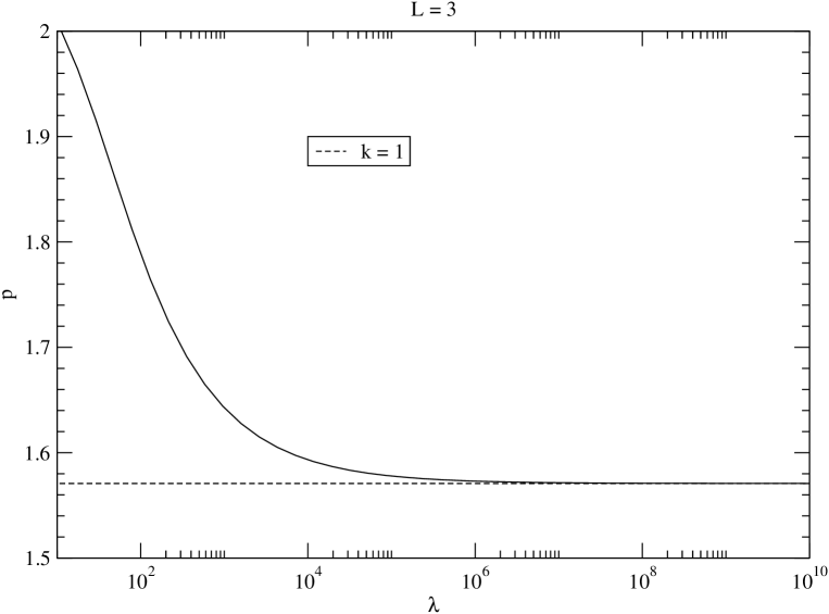
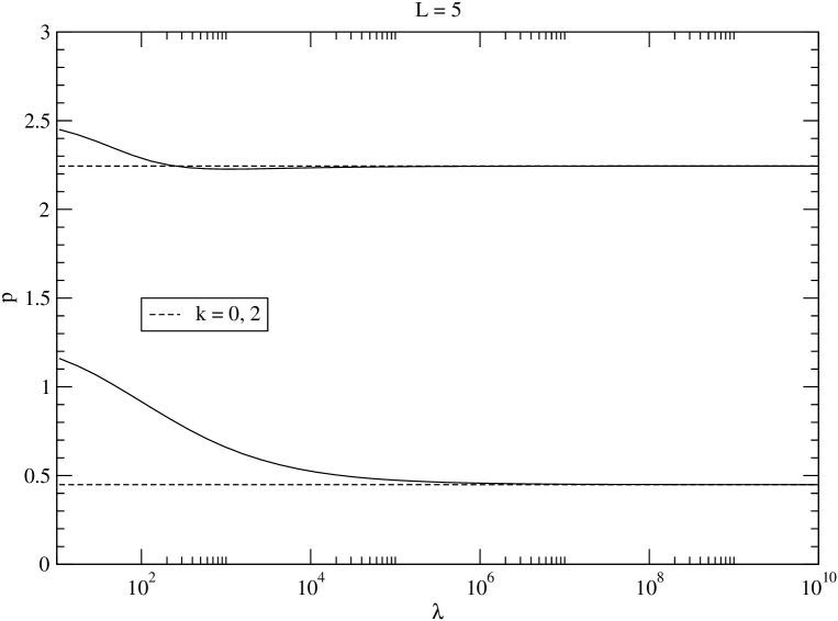
Figure 3: Positive Bethe momentum at $L=3,5$. The dashed lines are the analytical prediction.

Data for $L=3$ and $L=5$ are reported in Fig. (3); they confirm the Ansatz (22). We show the positive Bethe momentum and the prediction with $k=1$ for $L=3$, and $k=0,2$ for $L=5$. Notice that convergence is achieved at quite large $\lambda$.

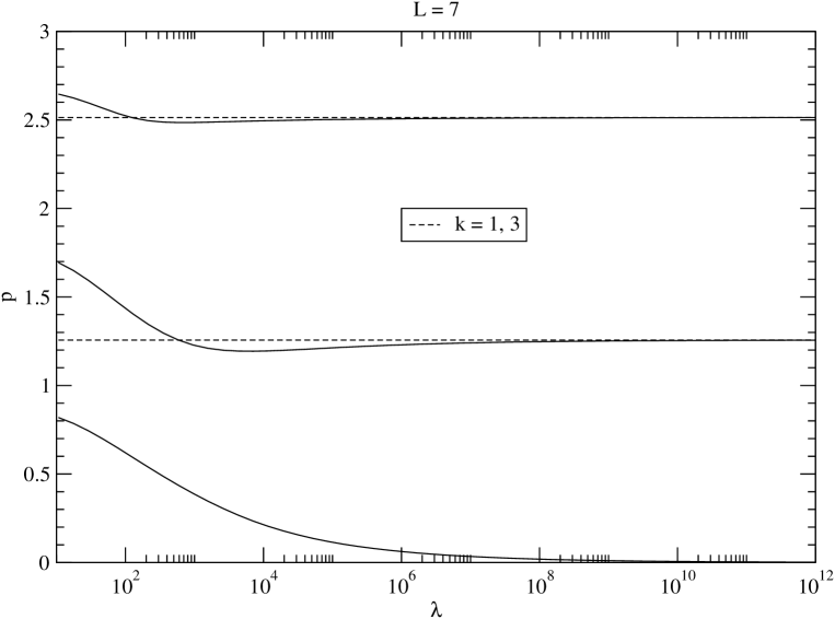
Figure 4: Positive and vanishing Bethe momenta at $L=7$. The dashed lines are the analytical predictions.

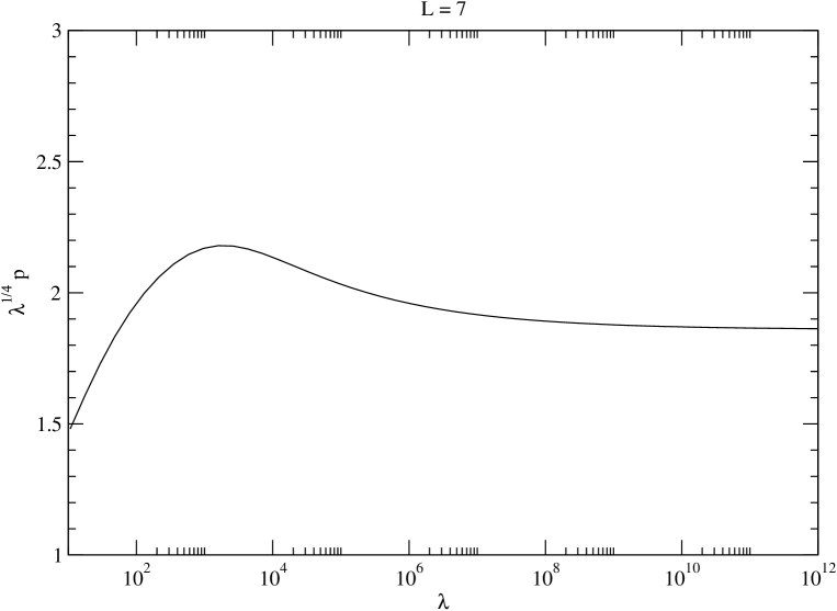
Figure 5: $\lambda^{-1/4}$ scaling of the vanishing momentum at $L=7$.

At $L=7$, the Bethe momenta are shown in Fig. (4). Here, something new happens. One of the Bethe momenta tends to zero. Nevertheless, the Ansatz (22) is still working, with $k=0,2$. The reason is that the vanishing momentum tends to zero like $\lambda^{-1/4}$ (case II) and the limiting form of the GBA equations is the same as it would be in case I. The asymptotic form of the vanishing momentum is illustrated in Fig. (5).

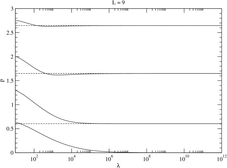
Figure 6: Positive and vanishing Bethe momenta at $L=9$. The dashed lines are the analytical predictions.

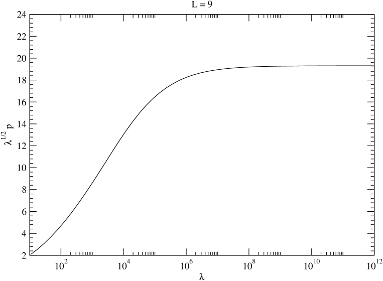
Figure 7: $\lambda^{-1/2}$ scaling of the vanishing momentum at $L=9$.

At $L=9$, the Bethe momenta are shown in Fig. (6). Here again one of the momenta tends to zero. Now, the Ansatz (22) fails to predict the correct asymptotic values of the non-vanishing momenta. Indeed, the vanishing momentum tends to zero like $\lambda^{-1/2}$ (case III) as shown in Fig. (7) and the limiting form of the GBA equations is changed. The dashed lines predicting the actual asymptotic non-zero $p$ are obtained as follows. Using again Eqs. (18), the GBA equation for any positive $p$ reads in the strong coupling limit ($L=9$)

$$e^{iLp}=e^{-3\,i\,p}\frac{1-\rho^{2}\,e^{-ip}}{1-\rho^{2}\,e^{ip}},\qquad\rho=\frac{\sqrt{2}\,\alpha}{1+\sqrt{1+2\alpha^{2}}},$$ (23)

where $\alpha$ appears in the asymptotic form of the vanishing momentum which is $\alpha/\sqrt{\lambda}$. For each $\rho$ we can determine the three positive $p$ nearest to the numerical asymptotic values. Then, we fix the parameter $\rho$ by using the strong coupling limit of the GBA equation for the vanishing momentum

$$1=\prod_{j=1,2,3}\frac{1-\rho\,e^{i\frac{p_{j}}{2}}}{1-\rho\,e^{-i\frac{p_{j}}{2}}}\frac{1+\rho\,e^{-i\frac{p_{j}}{2}}}{1+\rho\,e^{i\frac{p_{j}}{2}}},$$ (24)

The numerical solution is easily found. With 25 digits, it reads

$$\rho = 0.7261948032180057677773276,$$ (25)

$$p_{1} = 0.6047720145641787805731663,$$

$$p_{2} = 1.648738996485669279031225,$$

$$p_{3} = 2.646257150202204974776960.$$

The agreement, shown in Fig. (6) is excellent. In the following of this paper, we shall often have to solve equations like Eqs. (23-24). Whenever we claim that a numerical solution is easily found, we mean that standard packages, like Mathematica [40], can determine the solution with high precision in a straightforward way. For simplicity, we shall give just a relatively small number of digits for such results, but in all cases, we have checked their stability by increasing the precision and checking that the result is unchanged.

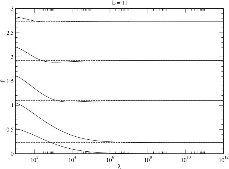
Figure 8: Positive and vanishing Bethe momenta at $L=11$. The dashed lines are the analytical predictions.

At $L=11$, the Bethe momenta are shown in Fig. (8). Here again one of the momenta tends to zero like $\lambda^{-1/2}$ (case III) and the limiting form of the GBA equations is changed. As before, we can compute the dashed lines showing the asymptotic non-zero $p$. The GBA equations for the positive $p$ read ($L=11$)

$$e^{iLp}=-e^{-4\,i\,p}\frac{1-\rho^{2}\,e^{-ip}}{1-\rho^{2}\,e^{ip}},$$ (26)

Again, for each $\rho$ we can determine the four positive $p$ nearest to the numerical asymptotic values. Then, $\rho$ is fixed by the GBA equation for the vanishing momentum which reads

$$1=\prod_{j=1,2,3,4}\frac{1-\rho\,e^{i\frac{p_{j}}{2}}}{1-\rho\,e^{-i\frac{p_{j}}{2}}}\frac{1+\rho\,e^{-i\frac{p_{j}}{2}}}{1+\rho\,e^{i\frac{p_{j}}{2}}},$$ (27)

The solution is now

$$\rho = 0.616048,$$ (28)

$$p_{1} = 0.227432,$$

$$p_{2} = 1.09891,$$

$$p_{3} = 1.92557,$$

$$p_{4} = 2.73741.$$

The agreement is shown in Fig. (8).

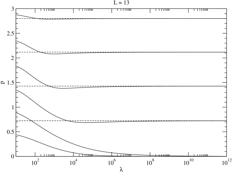
Figure 9: Positive and (two) vanishing Bethe momenta at $L=13$. The dashed lines are the analytical predictions.

At $L=13$, the Bethe momenta are shown in Fig. (9). Here two momenta tend to zero, one like $\lambda^{-1/2}$ and the other like $\lambda^{-1/4}$. We repeat the exercise of computing the asymptotic $p$. The GBA equation for the positive $p$ reads ($L=13$)

$$e^{iLp}=e^{-5\,i\,p}\frac{1-\rho^{2}\,e^{-ip}}{1-\rho^{2}\,e^{ip}},$$ (29)

For each $\rho$ we can determine the four positive $p$ nearest to the numerical asymptotic values. Then, we fix the parameter $\rho$ as before by the GBA equation for the vanishing momentum which reads

$$1=\prod_{j=1,2,3,4}\frac{1-\rho\,e^{i\frac{p_{j}}{2}}}{1-\rho\,e^{-i\frac{p_{j}}{2}}}\frac{1+\rho\,e^{-i\frac{p_{j}}{2}}}{1+\rho\,e^{i\frac{p_{j}}{2}}},$$ (30)

The solution is

$$\rho = 0.53244,$$

$$p_{1} = 0.72414,$$

$$p_{2} = 1.42787,$$ (31)

$$p_{3} = 2.11751,$$

$$p_{4} = 2.80082.$$

The agreement is shown in Fig. (9).

If $L$ is further increased, the pattern of vanishing and non vanishing momenta turns out to be quite regular. In the following table we show for each $L$ the number $N_{1/4}$ of positive momenta vanishing like $\lambda^{-1/4}$ and the number $N_{1/2}$ of those vanishing like $\lambda^{-1/2}$.

$L$	7	9	11	13	15	17	19	21	23	25	27	29	$\cdots$
$N_{\frac{1}{2}}$	0	1	1	1	2	2	2	3	3	3	4	4	$\cdots$
$N_{\frac{1}{4}}$	1	0	0	1	0	0	1	0	0	1	0	0	$\cdots$

Table 1: Periodicity of the number of vanishing Bethe momenta.

The general formulas expressing the $\mathbb{Z}_{3}$ regularity of the Table are

$$N_{\frac{1}{2}} = \lfloor\frac{L-1}{6}\rfloor-1+\left\{\begin{array}[]{ll}0,&\displaystyle\frac{L-1}{2}\,\mbox{mod}\,3=0,\\ \\ 1,&\mbox{otherwise}\end{array}\right.$$ (35)

$$N_{\frac{1}{4}} = \left\{\begin{array}[]{ll}1,&\displaystyle\frac{L-1}{2}\,\mbox{mod}\,3=0,\\ \\ 0,&\mbox{otherwise}\end{array}\right.$$ (39)

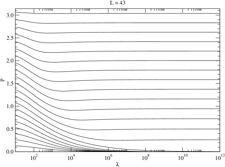
Figure 10: Positive and (seven) vanishing Bethe momenta at $L=43$.

For instance, if $L=43$ we expect 6 momenta vanishing like $\lambda^{-1/2}$ and one like $\lambda^{-1/4}$. The full set of momenta is shown in Fig. (10). It can be checked that the vanishing momenta have precisely these asymptotic behaviors.

2.2.4 Asymptotic form of $\Delta$

The asymptotic form of the anomalous dimension at fixed $L$ and large $\lambda$ is

$$\frac{\Delta}{L}\sim c_{L}\,\sqrt{\lambda}\qquad{\rm with}\ c_{L}=\frac{1}{L\,\pi}\sum_{k=1}^{L}\left|\sin\frac{p_{k}}{2}\right|,$$ (40)

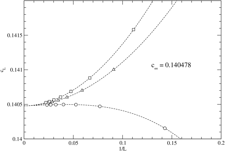
Figure 11: Determination of the prefactor $c_{\infty}$ associated with the leading term in the strong coupling expansion of the anomalous dimension predicted by the GBA equations. As explained in the text, the three curves are subsequences of lattice length with $((L-1)/2)\,{\rm mod}\,3=0,1,2$.

where the $p_{k}$ are the asymptotic non-zero values of the Bethe momenta. Due to the above periodicity, we can estimate $c_{\infty}$ by considering separately our data for $c_{L}$ for the three values of $((L-1)/2)\,{\rm mod}\,3$. The result from a fit of the data at $L>5$ by using a cubic polynomial in $1/L$ are shown in Fig. (11). The three subsequences have clearly the same limit. We find

$$c_{\infty}=0.1405(1),$$ (41)

where the error is a conservative estimate of the finite $L$ fit.

A remark about the order of the two limits $L,\lambda\to\infty$ is in order. We applied the resummation algorithm to estimate the leading term at large $\lambda$ of $\lim_{L\to\infty}\Delta/L$. Here, solving the GBA equations, we are fixing $L$ and taking the large $\lambda$ leading term $\sim c_{L}\sqrt{\lambda}$. Then, we evaluate $c_{\infty}=\lim_{L\to\infty}c_{L}$. Therefore, the double limit $L,\lambda\to\infty$ is taken in two different orders. Nevertheless, the agreement of the leading term in the two calculations is not surprising. This is precisely what happens for the AF state in the $\mathfrak{su}(2)$ sector. There, one can start from Eq. (1) and take after the $\lambda\to\infty$ limit. Alternatively, one can take the large $\lambda$ limit at fixed $L$, e.g. in the Hubbard model formulation. The result for the first three terms in the expansion is the same as discussed in [14].

3 The string Bethe Ansatz equations for the highest state in the $\mathfrak{su}(1|1)$ sector

The analysis of the GBA equations is certainly interesting, but the ultimate goal is the comparison with string theory. As discussed in the Introduction, it is not clear to what extent the GBA predicts correct results at strong coupling. This question can be investigated by studying the string Bethe Ansatz equations [9, 10] expected to predict the correct strong coupling behavior of string states, at least at large $L$.

In order to write the SBA equations in a compact way, we define $x^{\pm}_{k}=x^{\pm}(p_{k})$ and $u_{k}=u(p_{k})$ where

$$u(p)=\frac{1}{2}\cot\frac{p}{2}\sqrt{1+8\,g^{2}\,\sin^{2}\frac{p}{2}}.$$ (42)

The string Bethe Ansatz equations are then

$$e^{i\,L\,p_{k}}=\prod_{j\neq k}\frac{\displaystyle 1-\frac{g^{2}}{2\,x^{+}_{k}\,x^{-}_{j}}}{\displaystyle 1-\frac{g^{2}}{2\,x^{-}_{k}\,x^{+}_{j}}}\,e^{i\vartheta(p_{k},p_{j})},$$ (43)

where the scattering phase $\vartheta$ is

$$e^{i\vartheta(p_{k},p_{j})}=\left(\frac{\displaystyle 1-\frac{g^{2}}{2\,x^{+}_{k}\,x^{-}_{j}}}{\displaystyle 1-\frac{g^{2}}{2\,x^{-}_{k}\,x^{+}_{j}}}\right)^{-2}\,\,\left(\frac{\displaystyle 1-\frac{g^{2}}{2\,x^{+}_{k}\,x^{-}_{j}}}{\displaystyle 1-\frac{g^{2}}{2\,x^{-}_{k}\,x^{-}_{j}}}\,\frac{\displaystyle 1-\frac{g^{2}}{2\,x^{-}_{k}\,x^{+}_{j}}}{\displaystyle 1-\frac{g^{2}}{2\,x^{+}_{k}\,x^{+}_{j}}}\right)^{2\,i\,(u_{k}-u_{j})}.$$ (44)

In logarithmic form we have

$$p_{k}=\frac{2\pi}{L}\,n_{k}-\frac{i}{L}\sum_{j\neq k}\left(-\log\frac{\displaystyle 1-\frac{g^{2}}{2\,x^{+}_{k}\,x^{-}_{j}}}{\displaystyle 1-\frac{g^{2}}{2\,x^{-}_{k}\,x^{+}_{j}}}+2\,i\,(u_{k}-u_{j})\log\frac{\displaystyle 1-\frac{g^{2}}{2\,x^{+}_{k}\,x^{-}_{j}}}{\displaystyle 1-\frac{g^{2}}{2\,x^{-}_{k}\,x^{-}_{j}}}\,\frac{\displaystyle 1-\frac{g^{2}}{2\,x^{-}_{k}\,x^{+}_{j}}}{\displaystyle 1-\frac{g^{2}}{2\,x^{+}_{k}\,x^{+}_{j}}}\right).$$ (45)

These equations are considerably more involved than the GBA ones. Nevertheless, we have been able to repeat step by step the previous analysis as we now discuss.

3.1 Weak coupling expansion and Weniger resummation

We repeat the semi-numerical algorithm that we followed for the weak coupling expansion of the GBA equations. We take again $L=35$ and obtain the result

$$\lim_{L\to\infty}\frac{\Delta^{\rm string}}{L}=\textstyle\frac{3}{2}+2\,g^{2}-4\,g^{4}+\frac{25}{2}g^{6}-\frac{601}{12}g^{8}+\frac{2849}{12}g^{10}-\frac{25141}{20}g^{12}+\frac{429809}{60}g^{14}-\frac{9022721}{210}g^{16}$$ (46)

$$\textstyle+\frac{149821573}{560}g^{18}-\frac{8640293477}{5040}g^{20}+\frac{1812303079883}{161280}g^{22}-\frac{88730558092937}{1182720}g^{24}$$

$$\textstyle+\frac{1804497110708207}{3548160}g^{26}-\frac{26846650998855167}{7687680}g^{28}+\frac{279571052498891591}{11531520}g^{30}$$

$$\textstyle-\frac{125402745492098095339}{738017280}g^{32}+\frac{9738744677918359729}{8110080}g^{34}-\frac{6703245537745284313789}{784143360}g^{36}$$

$$\textstyle+\frac{1024647660942740023729097}{16728391680}g^{38}-\frac{2525524043347946614344579101}{5721109954560}g^{40}$$

$$\textstyle+\frac{18296543439438265154466562553}{5721109954560}g^{42}-\frac{1331791971895366969823043659509}{57211099545600}g^{44}$$

$$\textstyle+\frac{9735683703553399316563746438049}{57211099545600}g^{46}-\frac{345964047352595964568301174322841}{277022166220800}g^{48}$$

$$\textstyle+\frac{48414229366853228412090322467734657}{5263421158195200}g^{50}-\frac{2689943057205158649159985079500991}{39574595174400}g^{52}$$

$$\textstyle+\frac{5303581496963536951888629403691895353}{10526842316390400}g^{54}$$

$$\textstyle-\frac{19710992154318324101213041165671461761}{5263421158195200}g^{56}$$

$$\textstyle+\frac{870504639734489849012829744121725553}{31190643900416}g^{58}$$

$$\textstyle-\frac{10693434560671288576899374290035763214898727}{51286775765454028800}g^{60}$$

$$\textstyle+\frac{76039980287752685716954083401449551327779}{48705390090649600}g^{62}$$

$$\textstyle-\frac{10643182102443547953784209313106048717253607517}{908508599273757081600}g^{64}$$

$$\textstyle+\frac{2240647681205846470476844290367422504232816365029}{25438240779665198284800}g^{66}$$

$$\textstyle-\frac{5626138712126728829417020286414076511813854415733}{8479413593221732761600}g^{68}+{\cal O}(g^{70}).$$

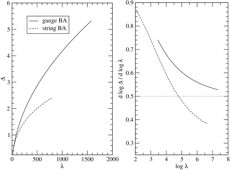
Figure 12: Comparison of the gauge/string Bethe Ansatz solutions as predicted by the Weniger resummation algorithm.

The Weniger resummation algorithm is convergent for $g^{2}\lesssim 10$. We show the resummed expression for $\Delta$ in the left panel of Fig. (12) for the gauge and string cases. The right panel shows the derivative

$$\frac{d}{d\log\lambda}\log\left(\lim_{L\to\infty}\frac{\Delta^{\rm string}}{L}\right),$$ (47)

which estimates at large $\lambda$ the exponent of the leading term. In the gauge case, it approaches the value $1/2$ at large $\lambda$, as we discussed. In the string case, the asymptotic value appears to be definitely smaller and the figure is qualitatively compatible with an asymptotic behavior $\sim\lambda^{1/4}$.

To support this conclusion, we have fitted the whole data with the functional form

$$\lim_{L\to\infty}\frac{\Delta^{\rm string}(\lambda)}{L}=c_{0}\,\lambda^{\nu}+c_{1}+c_{2}\,\lambda^{-\nu}+c_{3}\,\lambda^{-2\nu}.$$ (48)

The standard $\chi^{2}$ is a quantitative measure of the deviation from the supposed dependence on $\lambda$. The best values for the exponent $\nu$ are

$$\mbox{gauge BA}\,:\,\nu_{\rm fit}=0.496,\quad\mbox{string BA}\,:\,\nu_{\rm fit}=0.24,$$ (49)

which are very close to $1/2$ and $1/4$. If we now fix the exponent $\nu=1/2$ or $1/4$, we find the following $\chi^{2}$ for the two curves:

$$\begin{array}[]{ccc}\hline\cr\hline\cr\mbox{fixed exponent}&\nu=1/2&\nu=1/4\\ \hline\cr\hline\cr\\ \chi^{2}(\mbox{gauge BA})&2.3\cdot 10^{-5}&0.02\\ \\ \chi^{2}(\mbox{string BA})&0.03&1.4\cdot 10^{-4}\\ \\ \hline\cr\hline\cr\end{array}$$ (50)

As a conclusion, the resummed anomalous dimension favors the choice $\nu=1/4$ in the string case. The leading term with its numerical prefactor is

$$\lim_{L\to\infty}\frac{\Delta^{\rm string}}{L}=0.70(1)\,\lambda^{1/4}.$$ (51)

The prefactor is difficult to estimate and a better determination would require a stable resummation at larger $\lambda$.

While this result is quite pleasing, it must be criticized because of the moderate resummation range. Based on the weak coupling arguments [presented so far, it can not be ecluded that the string curve in the right panel of Fig. (12) could rise at larger $\lambda$ and flow back to the gauge value $1/2$. To pursue the analysis, as in the gauge case, we turn to a numerical iterative solution of the SBA equations. Indeed, it should be clear that several solutions are possible at strong coupling and the problem is again that of choosing the right one.

3.2 Exact solution at strong coupling

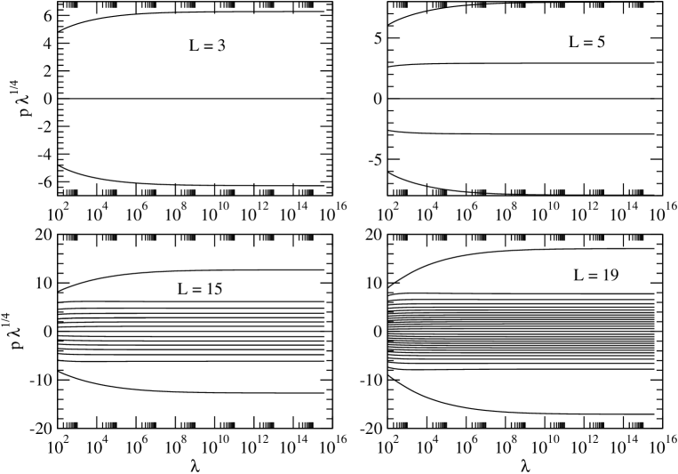
Figure 13: Solution of the SBA equations at four $L$. We show a plot of $\lambda^{1/4}p$ for the positive Bethe momenta.

We now determine the numerical solution of the SBA equations. We follow the same procedure we described for the gauge BA equations. The result is fully consistent with the weak coupling resummation: All Bethe momenta $p_{k}$ vanish at large $\lambda$ with an asymptotic behavior $p_{k}\sim\alpha_{k}\,\lambda^{-1/4}$ for all $p_{k}$! We illustrate this noticeable result by showing in Fig. (13) the evolution of Bethe momenta scaled by $\lambda^{1/4}$ in the four cases $L=3,5,15,29$.

The coefficients $\alpha_{k}$ are symmetrically distributed around zero. Qualitatively, $L-2$ coefficients $\alpha_{k}$ are almost evenly spaced around zero. Two special momenta have instead coefficients $\alpha_{k}$ well separated from the central band. Looking in more details at the explicit solution, one finds that the $\alpha_{k}$ in the central band have a non-trivial asymptotic density. The analysis of the large $L$ form of this density if deferred to future work.

It is not difficult to find an exact equation for the asymptotic coefficients $\alpha_{k}$. As we said, one of them is zero, $(L-1)/2$ are positive, and $(L-1)/2$ are opposite to the positive ones. Expanding the SBA equations at large $\lambda$ is a bit tricky but straightforward. We obtain the following equation determining the positive $\alpha_{k}>0$

$$\exp\left(\frac{i}{2\pi}\,\alpha_{k}\sum_{\alpha_{j}>0}\alpha_{j}\right) = \mathop{\prod_{\alpha_{j}>0}}_{j\neq k}\frac{-\frac{i}{2}(\alpha_{k}-\alpha_{j})+2\pi(\alpha_{k}^{-1}+\alpha_{j}^{-1})}{\frac{i}{2}(\alpha_{k}-\alpha_{j})+2\pi(\alpha_{k}^{-1}+\alpha_{j}^{-1})}\,\times$$ (52)

$$\times \left|\frac{\frac{i}{2}(\alpha_{k}-\alpha_{j})+2\pi(\alpha_{k}^{-1}+\alpha_{j}^{-1})}{-\frac{i}{2}(\alpha_{k}+\alpha_{j})+2\pi(\alpha_{k}^{-1}+\alpha_{j}^{-1})}\right|^{4i(h(\alpha_{k})-h(\alpha_{j}))}$$

$$h(\alpha) = \frac{\pi}{\alpha^{2}}-\frac{\alpha^{2}}{16\pi}.$$

where in the l.h.s. the sum includes the case $j=k$.

Although Eq. (52) is rather complicated, it can be solved numerically without difficulties, at least starting from the numerical $p$ obtained at a reasonably large $\lambda$. As an example, at $L=5,7,9$ we find the following (numerical) solutions

$$\begin{array}[]{ccc}L=5&&\\ \hline\cr\alpha_{1}&=&2.9213116645,\\ \alpha_{2}&=&7.9614845209,\end{array}\quad\begin{array}[]{ccc}L=7&&\\ \hline\cr\alpha_{1}&=&2.1234902933,\\ \alpha_{2}&=&4.0857786417,\\ \alpha_{3}&=&9.1813290270,\end{array}\quad\begin{array}[]{ccc}L=9&&\\ \hline\cr\alpha_{1}&=&1.6905819725,\\ \alpha_{2}&=&3.1495210704,\\ \alpha_{3}&=&4.8259074880,\\ \alpha_{4}&=&10.203166001\end{array}$$ (53)

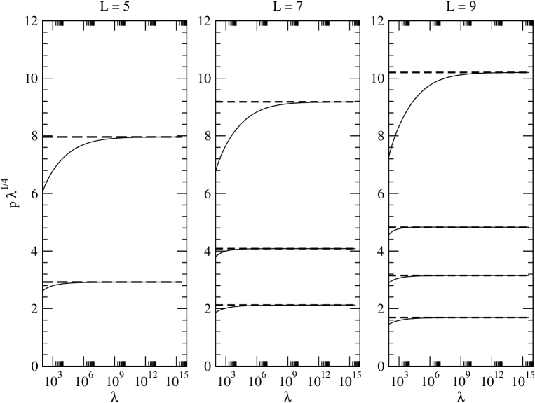
Figure 14: Check of the finite $L$ prediction of asymptotic coefficients $\alpha_{k}$ from the solution of Eq. (52).

These values are in perfect agreement with the numerical solution of the string Bethe Ansatz equations as illustrated in Fig. (14).

Actually, if we are interested in the asymptotic form of $\Delta^{\rm string}$, we do not need the full information encoded in the $\alpha_{k}$, but just their sum. Indeed,

$$\frac{\Delta^{\rm string}}{L}\sim c_{L}\,\lambda^{1/4},$$ (54)

where

$$c_{L}=\frac{1}{2\,L\,\pi}\sum_{k=1}^{L}\left|\alpha_{k}\right|=\frac{1}{L\pi}\sum_{\alpha_{k}>0}\alpha_{k}.$$ (55)

We now take the product of Eqs. (52). The right hand sides cancel perfectly. Evaluating the product of the left hand sides we obtain

$$\exp\left[\frac{i}{2\pi}\left(\sum_{\alpha_{j}>0}\alpha_{j}\right)^{2}\right]=1,\quad\Longrightarrow\quad\left(\sum_{\alpha_{j}>0}\alpha_{j}\right)^{2}=(2\pi)^{2}\,N_{L},$$ (56)

where $N_{L}\in\mathbb{N}$. These integers can be determined by solving Eqs. (52) at a certain $L$. The starting point for Newton’s algorithm is taken from the solution of the SBA equations at a reasonably large $\lambda$. Given the solution for the $\alpha_{k}$ coefficients, we can compute $N_{L}$. Indeed, the solution of Eqs. (52) can be accomplished easily with an arbitrarily high number of digits and the identification of the integer $N_{L}$ is totally straightforward and unambiguous.

The first values of $N_{L}$ are

$$\begin{array}[]{cccccccccccc}L&:&5&7&9&11&13&15&17&19&21&\dots\\ N_{L}&:&3&6&10&15&21&28&36&45&55&\dots\end{array}$$ (57)

The following simple formula holds

$$N_{L}=\frac{1}{8}(L^{2}-1),$$ (58)

leading to the prediction

$$c_{L}=\frac{1}{L\pi}\sum_{\alpha_{k}>0}\alpha_{k}=\frac{1}{L\pi}\,2\pi\sqrt{N_{L}}=\frac{1}{\sqrt{2}}\left(1-\frac{1}{L^{2}}\right)^{1/2}.$$ (59)

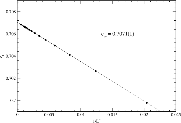
Figure 15: Numerical check of the prediction $c_{\infty}=1/\sqrt{2}$.

Now, we do not observe any particular $\mathbb{Z}_{3}$ structure. The values of $c_{L}$ are perfectly smooth as $L$ increases. As a further check of this analytical expression, we show in Fig. (15) the fit of $c_{\infty}$ with a simple quadratic polynomial in $1/L$. There is perfect agreement with the prediction

$$c_{\infty}=\frac{1}{\sqrt{2}}.$$ (60)

The numerical solution of the SBA equations and the resummation in the stable region $g^{2}\lesssim 10$ are in perfect agreement.

Of course, the appearance of the integer $N_{L}$ in the asymptotic form of $\Delta$ at large $\lambda$ is not surprising. Indeed, this is a general feature of the SBA equations as discussed in [21]. If the Bethe momenta vanish like $\lambda^{-1/4}$ at large $\lambda$, then the asymptotic form of $\Delta$ is

$$\Delta\sim 2\,\sqrt{n}\,\lambda^{1/4},$$ (61)

where $n$ is a sum of mode numbers. This is the celebrated string prediction of [2] where $n$ is the level of a massive string state. The calculation that we have described identifies the precise value of $n\equiv N_{L}$ for the state dual to the highest operator in the $\mathfrak{su}(1|1)$ sector.

4 The gauge Bethe Ansatz equations for the AF state in the $\mathfrak{su}(2)$ sector

It is straightforward to extend the analysis to the highest state in the $\mathfrak{su}(2)$ sector. The gauge Bethe Ansatz equations read

$$e^{i\,L\,p_{k}}=\prod_{j\neq k}\frac{x^{+}(p_{k})-x^{-}(p_{j})}{x^{-}(p_{k})-x^{+}(p_{j})}\,\frac{\displaystyle 1-\frac{g^{2}}{2\,x^{+}(p_{k})\,x^{-}(p_{j})}}{\displaystyle 1-\frac{g^{2}}{2\,x^{-}(p_{k})\,x^{+}(p_{j})}},\qquad k=1,\dots,L,$$ (62)

Now, we consider $L\in 2\,\mathbb{N}$.

At $g=0$ the above equations reduce to those of the Heisenberg model. The Bethe momenta $p_{k}$ are non-trivial and can be determined numerically at each $L$ as follows. At $g=0$ we have $u_{k}=\frac{1}{2}\cot\frac{p_{k}}{2}$. The variables $u_{k}$ can be determined by solving (e.g. iteratively)

$$2\pi\,J_{k}=2\sum_{j=1}^{L}\arctan(u_{k}-u_{j})-4\,L\arctan(2\,u_{k}),$$ (63)

where the Bethe quantum numbers $\{J_{k}\}$ for the AF state are

$$\{J_{k}\}=\left\{-\frac{L-1}{2},-\frac{L-3}{2},\dots,\frac{L-3}{2},\frac{L-1}{2}\right\}.$$ (64)

Here, it is not useful to compute the weak coupling expansion of $\Delta$. Indeed, due to the appearance of the non-trivial one-loop Bethe roots, all the coefficients of the expansion depend on $L$.

On the other hand, we can integrate numerically the equations. The result is not surprising and could be expected on the basis of the Hubbard model solution at finite $L$ discussed in [14]. At large $\lambda$, all Bethe momenta flow to constant values $p_{k}\to\overline{p}_{k}$ given by

$$\{\overline{p}_{1},\dots,\overline{p}_{L}\}=\left\{\pm\frac{\pi}{L},\pm\frac{3\pi}{L},\pm\frac{5\pi}{L},\dots,\pm\frac{L-1}{L}\pi\right\}.$$ (65)

Hence, the asymptotic form of the anomalous dimension is

$$\frac{\Delta}{2L} \sim \frac{1}{2L}\frac{\sqrt{\lambda}}{\pi}\sum_{\overline{p}}\left|\sin\frac{\overline{p}}{2}\right|=$$ (66)

$$= \frac{\sqrt{\lambda}}{L\,\pi}\sum_{\overline{p}>0}\sin\frac{\overline{p}}{2}=\frac{\sqrt{\lambda}}{L\,\pi}\sum_{s=0}^{L/2-1}\sin\frac{(2s+1)\pi}{2L}=\frac{\sqrt{\lambda}}{2\,\pi\,L\,\sin\frac{\pi}{2L}}$$ (67)

In particular, taking $L\to\infty$ we find

$$\lim_{L\to\infty}\frac{\Delta}{2L}=\frac{\sqrt{\lambda}}{\pi^{2}}+\dots.$$ (68)

The factor $2L$ in the scaled anomalous dimension is the correct one, i.e. the length of the associated lattice model. Indeed, in the $\mathfrak{su}(2)$ sector, the spin zero cyclic state associated with the AF state with $L$ Bethe momenta has $2L$ spins, $L$ with spin up and $L$ with spin down.

We remark that the above leading term is obtained both from the GBA equations and from the Hubbard model. It is quite interesting to see what happens at the level of string Bethe Ansatz equations.

5 The string Bethe Ansatz equations for the AF state in the $\mathfrak{su}(2)$ sector

The string Bethe Ansatz equations in the $\mathfrak{su}(2)$ sector are modified by the same universal dressing factor we introduced in the $\mathfrak{su}(1|1)$ sector. Thus, they read

$$e^{i\,L\,p_{k}}=\prod_{j\neq k}\frac{x^{+}(p_{k})-x^{-}(p_{j})}{x^{-}(p_{k})-x^{+}(p_{j})}\,\frac{\displaystyle 1-\frac{g^{2}}{2\,x^{+}(p_{k})\,x^{-}(p_{j})}}{\displaystyle 1-\frac{g^{2}}{2\,x^{-}(p_{k})\,x^{+}(p_{j})}}\,e^{i\vartheta(p_{k},p_{j})},$$ (69)

where the scattering phase $\vartheta(p_{k},p_{j})$ has been defined in Eq. (44).

We solve numerically these equations and the outcome is that all Bethe momenta vanish like $p_{k}\to\alpha_{k}\lambda^{-1/4}$ precisely as in the $\mathfrak{su}(1|1)$ case. Again we can work out an exact equation for the asymptotic coefficients $\{\alpha_{k}\}$. Taking the limit of the SBA equation we find the following modified form of Eq. (52)

$$\exp\left(\frac{i}{2\pi}\,\alpha_{k}\sum_{\alpha_{j}>0}\alpha_{j}\right)=$$ (70)

$$\mathop{\prod_{\alpha_{j}>0}}_{j\neq k}\frac{\frac{i}{2}(\alpha_{k}+\alpha_{j})+2\pi(\alpha_{k}^{-1}-\alpha_{j}^{-1})}{-\frac{i}{2}(\alpha_{k}+\alpha_{j})+2\pi(\alpha_{k}^{-1}-\alpha_{j}^{-1})}\,\frac{-\frac{i}{2}(\alpha_{k}-\alpha_{j})+2\pi(\alpha_{k}^{-1}+\alpha_{j}^{-1})}{\frac{i}{2}(\alpha_{k}-\alpha_{j})+2\pi(\alpha_{k}^{-1}+\alpha_{j}^{-1})}\,\times$$

$$\times \left|\frac{\frac{i}{2}(\alpha_{k}-\alpha_{j})+2\pi(\alpha_{k}^{-1}+\alpha_{j}^{-1})}{-\frac{i}{2}(\alpha_{k}+\alpha_{j})+2\pi(\alpha_{k}^{-1}+\alpha_{j}^{-1})}\right|^{4i(h(\alpha_{k})-h(\alpha_{j}))}$$

$$h(\alpha) = \frac{\pi}{\alpha^{2}}-\frac{\alpha^{2}}{16\pi}.$$

where in the l.h.s. the sum includes the case $j=k$.

As in the $\mathfrak{su}(1|1)$ sector, we can solve numerically this equation to cross check the numerical solution of the SBA equations. For instance, at $L=8$ we have four positive vanishing momenta and the above equation predicts

$$\alpha_{1} = 2.7192199579,$$ (71)

$$\alpha_{2} = 4.1578685742,$$

$$\alpha_{3} = 5.7295537708,$$

$$\alpha_{4} = 12.5260989258.$$

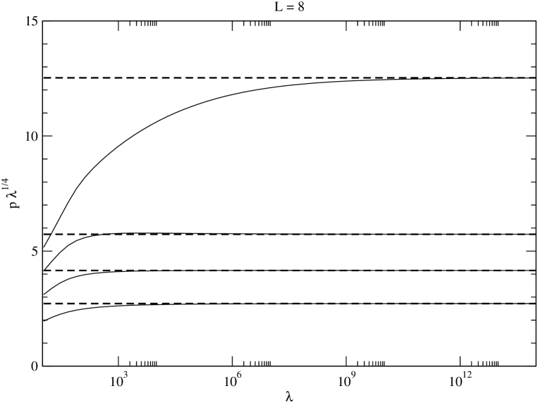
Figure 16: Check of the $L=8$ prediction of asymptotic coefficients $\alpha_{k}$ from the solution of Eq. (70).

The actual comparison with the solution of the SBA equations is shown in Fig. (16). To find the asymptotic expression of the anomalous dimension we can follow the same strategy as we did in the $\mathfrak{su}(1|1)$ sector. The extra factors in Eq. (70) also cancel when all the equations are multiplied together. Hence, we find again the fundamental relation

$$\left(\sum_{\alpha_{j}>0}\alpha_{j}\right)^{2}=(2\pi)^{2}\,N_{L},$$ (72)

with a different sequence $N_{L}$. Evaluating the solution to Eq. (70) we find the table

$$\begin{array}[]{cccccccccccc}L&:&4&6&8&10&12&14&16&18&20&\dots\\ N_{L}&:&4&9&16&25&36&49&64&81&100&\dots\end{array}$$ (73)

Hence, the following simple formula holds

$$N_{L}=\frac{1}{4}\,L^{2}$$ (74)

leading to the prediction

$$\frac{\Delta^{\rm string}}{2L}\sim c_{L}\,\lambda^{1/4},$$ (75)

with

$$c_{L}=\frac{1}{2\,L\,\pi}\sum_{\alpha_{k}>0}\alpha_{k}=\frac{1}{2\,L\,\pi}(2\pi)\frac{L}{2}=\frac{1}{2}.$$ (76)

This is an exact result holding at any finite $L$. For instance, it can be checked that it is valid for the $L=8$ solution up to the quoted accuracy.

Again, the integer $N_{L}$ appears in the asymptotic expression for $\Delta$ at large $\lambda$ in the form

$$\Delta\sim 2\,\sqrt{N_{L}}\,\lambda^{1/4},$$ (77)

identifying $N_{L}$ with the level of the massive string state dual to the AF operator.

6 Discussion

Quantitative tests of AdS/CFT require a perturbative window allowing reliable calculations on both sides of the correspondence. Such a window does not exist for generic sectors of the spectrum, but is available for semiclassical string states with large quantum numbers. In these BMN-like limits, a perturbative check of AdS/CFT at weak effective ’t Hooft coupling can be attempted, but is known to fail at three loops. This discrepancy can be seen as a limitation to our capability of capturing the strong quantum dynamics of string theory beyond the BMN limit, i.e. the small $\lambda$ regime for states with fixed finite classical dimension $L$.

On one hand, the GBA equations are effective in computing all-loop perturbative gauge theory properties, like anomalous dimensions. However, the implicit order of limits ($L\to\infty$ after $\lambda\to 0$) spoils the agreement with string calculations beyond two loops. On the other hand, the SBA equations are valid at large $\lambda$, but already the leading quantum corrections are known to receive important and non-trivial corrections at small $\lambda$ [22, 23, 24, 25], not yet under full control despite recent progresses [33, 34].

At large $\lambda$, the picture is quite different. In principle, the GBA equations should not be trusted because the wrapping terms cannot be neglected. Instead, the SBA equations are expected to match string calculations, including leading quantum corrections. Hence, we can make predictions on the string side, but we cannot test the AdS/CFT correspondence. Actually, this general statement is very conservative. Specific cases must be treated with care and a matching between the solutions of the two sets of equations is possible. Indeed, the structural difference between GBA and SBA equations lies only in the dressing scattering phase Eq. (44) and the relevance of this extra term should be considered case by case.

Important examples of such exceptions can be found in various BMN-like limits. For instance, the exact all loop expression of plane wave string levels reads in the strict BMN limit

$$\Delta_{M}-J=\sum_{k=1}^{M}\sqrt{1+n_{k}^{2}\,\lambda^{\prime}},\qquad\lambda^{\prime}=\frac{\lambda}{J^{2}},\ J\to\infty,$$ (78)

and scales like $(\lambda^{\prime})^{1/2}$ at large $\lambda^{\prime}$. This result is valid both in the framework of GBA [11] and SBA [21] equations. In this case, the matching of the two predictions is due to the fact that the impurities are fixed in number and their diluteness prevents scattering effects in the thermodynamical limit. A related example is the Hofman-Maldacena limit which also displays asymptotic $(\lambda^{\prime})^{1/2}$ scaling laws closely related to the BMN case [43, 44, 46, 45, 47]. Again, in the Hofman-Maldacena limit, the dressing factor in the SBA equations has been shown to decouple, making the prediction from the GBA exact, at least in the thermodynamical limit [48].

These examples should be regarded as exceptions, precisely because the irrelevance of the dressing phase is not expected to be generic feature. A more involved example where an explicit strong coupling discrepancy appears is the folded string (FS) solution [27] in the $\mathfrak{su}(2)$ sector. The energy of this solution is a function $\Delta_{\rm FS}(\lambda,J)$. In the AdS/CFT correspondence, it must be matched with the anomalous dimension of an operator with $L=2J$ constituent scalar fields. The scaling operator is well known, at least in the $L\to\infty$ limit and is the double contour solution of the GBA equations described in [37]. It has been studied in some details also in the Hubbard model formulation [14]. Setting, as usual $\lambda^{\prime}=\lambda/J^{2}$ we have

$$\lim_{J\to\infty}\frac{\Delta^{\rm string}_{\rm FS}(\lambda^{\prime}\,J^{2},J)}{2J}=f(\lambda^{\prime}),$$ (79)

where the function $f(\lambda^{\prime})$ is explicitely known. The leading term is obtained by expanding at large $\lambda^{\prime}$:

$$f(\lambda^{\prime})\sim\frac{1}{\sqrt{2}}\,(\lambda^{\prime})^{1/4}.$$ (80)

One can ask whether it is possible to reproduce Eq. (80) with the GBA equations. The anomalous dimension $\Delta^{\rm gauge}_{\rm FS}$ of the double contour solution is known at strong coupling and finite $J$ in the Hubbard model GBA equations [14]. It reads

$$\frac{\Delta_{\rm FS}^{\rm gauge}(\lambda,J)}{2J}\sim\frac{1}{\pi\sqrt{2}}\,\cos\frac{\pi}{4J}\,(\lambda^{\prime})^{1/2}\ \ \stackrel{{\scriptstyle J\to\infty}}{{\longrightarrow}}\ \ \frac{1}{\pi\sqrt{2}}\,(\lambda^{\prime})^{1/2}.$$ (81)

With the usual remarks about the order of limits, we see that the GBA/SBA equations predict an asymptotic behaviour $\sim(\lambda^{\prime})^{\nu}$ with $\nu=1/2$ and $1/4$ respectively. Here the number of impurities in the folded string solution gets large as $J\to\infty$ and their finite density makes the role of the dressing scattering phase non-trivial.

Following these remarks, it seems interesting to look at other explicit non-trivial examples where the GBA and SBA equations can be compared in the strong-coupling region. From a slightly different perspective, one is considering a special class of states and wonders about the role of the SBA scattering phase. Following this line of reasoning, this work analyzes the highest state in the $\mathfrak{su}(1|1)$ and $\mathfrak{su}(2)$ sectors of ${\cal N}=4$ SYM. We have been able to solve all ambiguities appearing in the strong coupling expansion of the Bethe Ansatz equations. Our results have been cross-checked with a resummation technique which is able to connect smoothly the weak- and strong-coupling regions. Our main results have already been summarized in Eqs. (5) and are repeated below for the reader’s advantage.

$$\begin{array}[]{ccl}\displaystyle\frac{\Delta_{\mathfrak{su}(2)}^{\rm gauge}}{2L}&=&\displaystyle\frac{1}{2\pi L\sin{\displaystyle\frac{\pi}{2L}}}\,\lambda^{1/2},\\ \\ \displaystyle\frac{\Delta_{\mathfrak{su}(1|1)}^{\rm gauge}}{L}&=&\displaystyle c_{L}\,\lambda^{1/2},\end{array}\qquad\begin{array}[]{ccl}\displaystyle\frac{\Delta_{\mathfrak{su}(2)}^{\rm string}}{2L}&=&\displaystyle\frac{1}{2}\,\lambda^{1/4},\\ \\ \displaystyle\frac{\Delta_{\mathfrak{su}(1|1)}^{\rm string}}{L}&=&\displaystyle\frac{1}{\sqrt{2}}\left(1-\frac{1}{L^{2}}\right)\,\lambda^{1/4},\end{array}$$ (82)

$$c_{L}\to 0.1405(1),\quad\mbox{as}\ L\to\infty.$$

The main outcome of our analysis is the following. For any fixed $L$, the highest states in the $\mathfrak{su}(2)$ or $\mathfrak{su}(1|1)$ sectors have a large $\lambda$ anomalous dimension scaling like $\Delta\sim\lambda^{\nu}$ where $\nu=1/2$ in the GBA equations and $\nu=1/4$ in the SBA equations. At large $\lambda$ (and $L$) the SBA equations can be trusted without subtleties. Hence, the $\lambda^{1/2}$ scaling predicted by the GBA equations is not a true feature of the highest states. Their anomalous dimension immediately scales like $\lambda^{1/4}$ and uniformly in $L$ as soon as they are treated by the string Bethe Ansatz equations.

We remark that our result is somewhat novel. Indeed, in the $\mathfrak{su}(2)$ sector, it is common lore to believe in the $\sqrt{\lambda}$ scaling of the AF operator, after its identification with the dual of the slow-string limit solution in [38]. From our analysis, we see that it is certainly possible to force the SBA equations to exhibit $\lambda^{1/2}$ scaling. However, this must be done by assuming a large $\lambda$ behavior of the Bethe momenta that is ruled out by the explicit solution of the equations, at least for the highest states.

Notice also that it is possible to quantize the superstring equations of motion after truncation to the $\mathfrak{su}(1|1)$ sector [49, 50]. The spectrum contains long string solutions with non-vanishing winding $w=\sum_{k}p_{k}$ with $\lambda^{1/2}$ scaling. On the contrary, short strings with vanishing winding exhibit the usual $\lambda^{1/4}$ scaling. The observed symmetry $p\to-p$ of Bethe momenta favors the $w=0$ option.

In conclusion, apart from the above mentioned special cases, it seems definitely dangerous to rely on the GBA equations to estimate the strong coupling limit of general states, as our analysis of the highest states has shown. Instead, the full solution of the SBA equations, even at the discussed semi-analytical level, appears to be an effective predictive tool. For instance, our result 

$$\begin{array}[]{lclcccl}\Delta^{\rm string}_{L,\mathfrak{su}(1|1)}&=&\displaystyle 2\sqrt{N_{L}}\,\lambda^{1/4},&&N_{L}&=&\displaystyle\frac{1}{8}(L^{2}-1),\\ \\ \Delta^{\rm string}_{L,\mathfrak{su}(2)}&=&\displaystyle 2\sqrt{N_{L}}\,\lambda^{1/4},&&N_{L}&=&\displaystyle\frac{1}{4}L^{2},\end{array}$$ (83)

gives a simple formula for the level of the string state dual to the highest state in the two compact sectors.

Appendix A The Weniger resummation algorithm

Given the power series

$$\lim_{L\to\infty}\frac{\Delta}{L}=\sum_{n\geq 0}c_{n}\,g^{2n},$$ (84)

we can evaluate the partial sums

$$s_{n}=\sum_{k=0}^{n}c_{k}.$$ (85)

From the partial sums, we form the Weniger approximants

$${\delta}_{n}\;=\;\frac{\displaystyle\sum_{j=0}^{n}\;(-1)^{j}\;{{n}\choose{j}}\;\frac{(1+j)_{n-1}}{(1+n)_{n-1}}\;\frac{s_{j}}{c_{j+1}}}{\displaystyle\sum_{j=0}^{n}\;(-1)^{j}\;{{n}\choose{j}}\;\frac{(1+j)_{n-1}}{(1+n)_{n-1}}\;\frac{1}{c_{j+1}}}\,,$$ (86)

where $(a)_{m}=\Gamma(a+m)/\Gamma(a)$ is the Pochhammer symbol. If $g^{2}$ is beyond the convergence radius, the partial sums do not converge and oscillate wildly. For better stability we have performed all calculations in exact arithmetics. If the Weniger algorithms succeeds in resumming the series, then the Weniger approximants converge.

References

- [1] J. M. Maldacena, The large limit of superconformal field theories and supergravity, Adv. Theor. Math. Phys. 2, 231 (1998) [Int. J. Theor. Phys. 38, 1113 (1999)] [arXiv:hep-th/9711200].
- [2] S. S. Gubser, I. R. Klebanov and A. M. Polyakov, Gauge theory correlators from non-critical string theory, Phys. Lett. B 428, 105 (1998) [arXiv:hep-th/9802109].
- [3] E. Witten, Anti-de Sitter space and holography, Adv. Theor. Math. Phys. 2, 253 (1998) [arXiv:hep-th/9802150].
- [4] V. A. Kazakov, A. Marshakov, J. A. Minahan and K. Zarembo, Classical / quantum integrability in AdS/CFT, JHEP 0405, 024 (2004) [arXiv:hep-th/0402207].
- [5] I. R. Klebanov, TASI lectures: Introduction to the AdS/CFT correspondence, arXiv:hep-th/0009139.
- [6] J. A. Minahan and K. Zarembo, The Bethe-Ansatz for super Yang-Mills, JHEP 0303, 013 (2003) [arXiv:hep-th/0212208].
- [7] N. Beisert, The complete one-loop dilatation operator of super Yang-Mills theory, Nucl. Phys. B 676, 3 (2004) [arXiv:hep-th/0307015].
- [8] N. Beisert, The dilatation operator of super Yang-Mills theory and integrability, Phys. Rept. 405, 1 (2005) [arXiv:hep-th/0407277].
- [9] M. Staudacher, The factorized S-matrix of CFT/AdS, JHEP 0505, 054 (2005) [arXiv:hep-th/0412188].
- [10] N. Beisert and M. Staudacher, Long-range PSU(2,24) Bethe ansaetze for gauge theory and strings, Nucl. Phys. B 727, 1 (2005) [arXiv:hep-th/0504190].
- [11] N. Beisert, V. Dippel and M. Staudacher, A novel long range spin chain and planar super Yang-Mills, JHEP 0407, 075 (2004) [arXiv:hep-th/0405001].
- [12] A. Rej, D. Serban and M. Staudacher, Planar gauge theory and the Hubbard model, JHEP 0603, 018 (2006) [arXiv:hep-th/0512077].
- [13] J. A. Minahan, Strong coupling from the Hubbard model, arXiv:hep-th/0603175.
- [14] M. Beccaria and C. Ortix, Strong coupling anomalous dimensions of super Yang-Mills, arXiv:hep-th/0606138.
- [15] D. Berenstein, J. M. Maldacena and H. Nastase, Strings in flat space and pp waves from super Yang Mills, JHEP 0204 (2002) 013, hep-th/0202021.
- [16] C. G. Callan, H. K. Lee, T. McLoughlin, J. H. Schwarz, I. J. Swanson and X. Wu, Quantizing string theory in AdS(5) x S**5: Beyond the pp-wave, Nucl. Phys. B 673, 3 (2003) [arXiv:hep-th/0307032].
- [17] C. G. Callan, T. McLoughlin and I. J. Swanson, Holography beyond the Penrose limit, Nucl. Phys. B 694, 115 (2004) [arXiv:hep-th/0404007].
- [18] C. G. Callan, T. McLoughlin and I. J. Swanson, Higher impurity AdS/CFT correspondence in the near-BMN limit, Nucl. Phys. B 700, 271 (2004) [arXiv:hep-th/0405153].
- [19] C. G. Callan, J. Heckman, T. McLoughlin and I. J. Swanson, Lattice super Yang-Mills: A virial approach to operator dimensions, Nucl. Phys. B 701, 180 (2004) [arXiv:hep-th/0407096].
- [20] D. Serban and M. Staudacher, Planar N = 4 gauge theory and the Inozemtsev long range spin chain, JHEP 0406, 001 (2004) [arXiv:hep-th/0401057].
- [21] G. Arutyunov, S. Frolov and M. Staudacher, Bethe Ansatz for quantum strings, JHEP 0410, 016 (2004) [arXiv:hep-th/0406256].
- [22] N. Beisert and A. A. Tseytlin, On quantum corrections to spinning strings and Bethe equations, Phys. Lett. B 629, 102 (2005) [arXiv:hep-th/0509084].
- [23] S. Schafer-Nameki, M. Zamaklar and K. Zarembo, Quantum corrections to spinning strings in and Bethe Ansatz: A comparative study, JHEP 0509, 051 (2005) [arXiv:hep-th/0507189].
- [24] S. Schafer-Nameki and M. Zamaklar, Stringy sums and corrections to the quantum string Bethe Ansatz, JHEP 0510, 044 (2005) [arXiv:hep-th/0509096].
- [25] S. Schafer-Nameki, Exact expressions for quantum corrections to spinning strings, arXiv:hep-th/0602214.
- [26] S. Frolov and A. A. Tseytlin, Multi-spin string solutions in , Nucl. Phys. B 668, 77 (2003) [arXiv:hep-th/0304255].
- [27] S. Frolov and A. A. Tseytlin, Rotating string solutions: AdS/CFT duality in non-supersymmetric sectors, Phys. Lett. B 570, 96 (2003) [arXiv:hep-th/0306143].
- [28] G. Arutyunov, S. Frolov, J. Russo and A. A. Tseytlin, Spinning strings in AdS(5) x S**5 and integrable systems, Nucl. Phys. B 671, 3 (2003) [arXiv:hep-th/0307191].
- [29] G. Arutyunov, J. Russo and A. A. Tseytlin, Spinning strings in AdS(5) x S**5: New integrable system relations, Phys. Rev. D 69, 086009 (2004) [arXiv:hep-th/0311004].
- [30] S. Frolov and A. A. Tseytlin, Quantizing three-spin string solution in AdS(5) x S**5, JHEP 0307, 016 (2003) [arXiv:hep-th/0306130].
- [31] S. A. Frolov, I. Y. Park and A. A. Tseytlin, On one-loop correction to energy of spinning strings in S(5), Phys. Rev. D 71, 026006 (2005) [arXiv:hep-th/0408187].
- [32] I. Y. Park, A. Tirziu and A. A. Tseytlin, Spinning strings in AdS(5) x S**5: One-loop correction to energy in SL(2) sector, JHEP 0503, 013 (2005) [arXiv:hep-th/0501203].
- [33] R. Hernandez and E. Lopez, Quantum corrections to the string Bethe ansatz, arXiv:hep-th/0603204.
- [34] L. Freyhult and C. Kristjansen, A universality test of the quantum string Bethe ansatz, Phys. Lett. B 638, 258 (2006) [arXiv:hep-th/0604069].
- [35] G. Arutyunov and A. A. Tseytlin, On highest-energy state in the sector of super Yang-Mills theory, JHEP 0605, 033 (2006) [arXiv:hep-th/0603113].
- [36] K. Zarembo, Antiferromagnetic operators in supersymmetric Yang-Mills theory, Phys. Lett. B 634, 552 (2006) [arXiv:hep-th/0512079].
- [37] S. Frolov and A. A. Tseytlin, Semiclassical quantization of rotating superstring in JHEP 0206, 007 (2002), hep-th/0204226. Multi-spin string solutions in , Nucl. Phys. B 668, 77 (2003), hep-th/0304255. N. Beisert, J. A. Minahan, M. Staudacher and K. Zarembo, Stringing spins and spinning strings, JHEP 0309, 010 (2003), hep-th/0306139. N. Beisert, S. Frolov, M. Staudacher and A. A. Tseytlin, Precision spectroscopy of AdS/CFT, JHEP 0310, 037 (2003), hep-th/0308117.
- [38] R. Roiban, A. Tirziu and A. A. Tseytlin, Slow-string limit and ’antiferromagnetic’ state in AdS/CFT, Phys. Rev. D 73, 066003 (2006) [arXiv:hep-th/0601074].
- [39] N. Beisert, The su(23) dynamic spin chain, Nucl. Phys. B 682, 487 (2004) [arXiv:hep-th/0310252].
- [40] Wolfram Research, Inc., Mathematica, Version 5.2, Champaign, IL (2005).
- [41] E. J. Weniger, Nonlinear sequence transformations for the acceleration of convergence and the summation of divergent series, Comp. Phys. Rep. 10, 189 (1989)
- [42] The Newton algorithm is available in the modern packages for symbolic/numerical calculations. A simple description of the Newton algorithm can be found in William H. Press (Editor), Saul A. Teukolsky (Editor), William T. Vetterling, Brian P. Flannery, Numerical Recipes in C++: The Art of Scientific Computing, Cambridge University Press; 2 edition (February 2002), ISBN: 0521750334.
- [43] D. M. Hofman and J. M. Maldacena, Giant magnons, arXiv:hep-th/0604135.
- [44] N. Dorey, Magnon bound states and the AdS/CFT correspondence, arXiv:hep-th/0604175.
- [45] M. Spradlin and A. Volovich, Dressing the giant magnon, arXiv:hep-th/0607009.
- [46] N. P. Bobev and R. C. Rashkov, Multispin giant magnons, arXiv:hep-th/0607018.
- [47] M. Kruczenski, J. Russo and A. A. Tseytlin, Spiky strings and giant magnons on S5, arXiv:hep-th/0607044.
- [48] J. A. Minahan, A. Tirziu and A. A. Tseytlin, Infinite spin limit of semiclassical string states, arXiv:hep-th/0606145.
- [49] L. F. Alday, G. Arutyunov and S. Frolov, New integrable system of 2dim fermions from strings on , JHEP 0601, 078 (2006) [arXiv:hep-th/0508140].
- [50] G. Arutyunov and S. Frolov, Uniform light-cone gauge for strings in : Solving su(11) sector, JHEP 0601, 055 (2006) [arXiv:hep-th/0510208].