IP/BBSR/2006-11
UV/IR Mixing in Noncommutative Field Theories and Open Closed String Duality

Abstract

In this paper we study the phenomenon of UV/IR mixing in noncommutative field theories from the point of view of world-sheet open-closed duality in string theory. New infrared divergences in noncommutative field theories arise as a result of integrating over high momentum modes in the loops. These are believed to come from integrating out additional bulk closed string modes. We analyse this issue in detail for the bosonic theory and further for the supersymmetric theory on the $C^{2}/Z_{2}$ orbifold. We elucidate on the exact role played by the constant background $B$-field in this correspondence.

1 Introduction

Dualities have played a very important role in the understanding of various issues in string theory. World-sheet duality in string theory have been observed since the early days of its formulation. It is now believed that this duality underlies the duality between the open and closed string theories. In certain backgrounds such as in AdS/CFT [1, 2], this manifests as the relation between only the massless open and closed string sectors. In this review we will study this world-sheet duality in a background antisymmetric two-form constant $B$-field.

Studies of open string dynamics in the background $B$-field have shown that the low energy dynamics is given by a gauge theory on noncommutative space-times [3, 4, 5, 6, 7]. Apart from this realisation of noncommutative gauge theory, quantum field theories on noncommutative space-times have independently been studied for a long time with a hope to cure the ultraviolet divergence problem in quantum field theories that arise in the continuum limit. The rationale for this being that discreteness of space time is inherent in any quantum formulation of gravity and that noncommutative space-time is one of the ways to achieve this [8][9]. Quantum field theories on noncommutative backgrounds are nonlocal and sometimes violate the conventional notions of local quantum field theories. Various aspects of these theories have been studied extensively over the past few years [10]. More often their embedding into string theory has led to a better understanding of these issues.

One of the well known generic features of these theories is the mixing of the ultraviolet and the infrared sectors contrary to the ordinary quantum field theories where they decouple [11]. Within the domain of quantum field theory it is thus important to see how the usual notions of Wilsonian Renormalisation Group fits into these models. A thorough analysis shows that an IR cut-off is necessary for the Wilsonian RG to make sense here, and with the IR cut-off usual renormalisation can be done [13]. The need for an IR cut-off in studying nonplanar anomalies in gauge theories has also been explored. See [14] and references therein.

Recently a different approach has been pursued that lead to the removal of UV/IR mixing in noncommutative field theories [15, 16]. The spin-statistics theorem however needs to be modified here and thus it is, not clear whether this is to be viewed as an inequivalent quantisation and therefore a different theory or a different cure to the infrared divergences (also see [17]). For other approaches addressing this issue of UV/IR mixing and hence renormalisation in noncommutative field theories see [18].

In this review we will study this phenomenon of mixing of UV and the IR sectors of noncommutative field theories from the point of view of world-sheet open closed string duality. The ultraviolet divergences in open string theory can be interpreted as closed string infrared divergence using the world-sheet duality. In the presence of the background $B$-field these divergences are regulated and thus a quantitative analysis can be made. The one-loop two point diagram for open strings is a cylinder with a modular parameter $t$ and vertex operator insertions at the boundaries. The two point one-loop noncommutative field theory diagram results in the Seiberg-Witten limit by keeping surviving terms in the integrand for the integral over $t$ for $t\rightarrow\infty$. This limit suppresses all contributions from massive modes in the loop. The resulting diagram is that of the gauge theory with massless propagating modes. This amplitude is usually divergent in the ultraviolet when integrated over $t$. The source of ultraviolet divergence is the same as that of those in string theory i.e. $t\rightarrow 0$. It is therefore natural to analyse the amplitude directly in this limit when only the low lying closed string exchanges contribute.

In the bosonic string theory setting, we will first analyse the two-point one loop amplitude for gauge bosons on the brane, in the closed string channel [32]. Though there are additional tachyonic divergences, we are able to show that the form of IR divergences with appropriate tensor structures can be extracted by considering only lowest lying modes (tachyonic and massless). We will further analyse the two point amplitude by studying massless closed string exchanges in background constant $B$-field.

It was observed that ultraviolet behaviour of the one loop gauge theory is same as that of the infrared due to massless closed string tree-level exchanges in nonconformal gauge theory with ${\cal N}=2$ supersymmetry [35]. The simplest way to realise this gauge theory is on fractional branes localised at the fixed point on $C^{2}/Z_{2}$. Various aspects of this duality have since been studied [36, 37, 38, 39, 40, 41, 42, 43]. In the next part of this analysis we will show that the UV/IR mixing phenomenon of ${\cal N}=2$ gauge theory can be naturally interpreted as a consequence of open-closed string duality in the presence of background $B$-field [33, 34].

This review is organised as follows. In Section 2 we give a brief review of open bosonic strings in background constant $B$-field and the appearance of noncommutative field theory as low-energy description of $D$-brane world volume dynamics. In Section 3, we study the one loop open string amplitude in the UV limit and write down the contribution from the lowest states. In Section 4, we analyse massless closed string exchanges in background $B$-field and reconstruct the massless contribution computed in Section 3. In Section 5 we study superstrings in $B$-field background and give a short review of strings on $C^{2}/Z_{2}$ orbifold and the massless spectrum of open strings ending on fractional $D_{3}$-brane localised at the fixed point and closed strings. In Section 6 we compute the two point function for one loop open strings in this orbifold background with the $B$-field turned on, and analyse it in the open and closed string channels. By taking the field theory limit, we show using open-closed string duality that the new IR divergent term from the nonplanar amplitude is exactly equal to the IR divergent contributions from massless closed string exchanges. In Section 7, we study massless closed string exchanges on $C^{2}/Z_{2}$ orbifold along the same lines as in Section 4. We conclude this article with discussions in Section 8.

Conventions: We will use capital letters $(M,N,...)$ to denote general space-time indices and small letters $(i,j,...)$ for coordinates along the $D$-brane. Small Greek letters $(\alpha,\beta...)$ will be used to denote indices for directions transverse to the brane.

2 Bosonic strings in background $B$-field and noncommutative field theory

In this section we give a short review of open string dynamics in the presence of constant background $B$-field leading to noncommutative field theory on the world volume of a $D$-brane [7]. In the presence of a constant background $B$-field, the world sheet action is given by,

$$S_{b}=\frac{1}{4\pi\alpha^{{}^{\prime}}}\int_{\Sigma}[g_{MN}\partial_{a}X^{M}\partial^{a}X^{N}-2\pi i\alpha^{{}^{\prime}}B_{MN}\epsilon^{ab}\partial_{a}X^{M}\partial_{b}X^{N}]$$ (2.1)

Consider a $D_{p}$ brane extending in the directions $1$ to $p$, such that, $B_{MN}\neq 0$ only for $M,N\leq p+1$ and $B_{MN}=0$ for $M\leq p+1,N>p$. The equation of motion gives the following boundary condition,

$$g_{MN}\partial_{n}X^{N}+2\pi i\alpha^{{}^{\prime}}B_{MN}\partial_{t}X^{N}|_{\partial\Sigma}=0$$ (2.2)

The world sheet propagator on the boundary of a disc satisfying this boundary condition is given by,

$${\cal G}(y,y^{{}^{\prime}})=-\alpha^{{}^{\prime}}G^{MN}\ln(y-y^{{}^{\prime}})^{2}+\frac{i}{2}\theta^{MN}\epsilon(y-y^{{}^{\prime}})$$ (2.3)

where, $\epsilon(\Delta y)$ is $1$ for $\Delta y>0$ and $-1$ for $\Delta y<0$. $G_{MN}$, $\theta_{MN}$ are given by,

$$G^{MN} = \left(\frac{1}{g+2\pi\alpha^{{}^{\prime}}B}g\frac{1}{g-2\pi\alpha^{{}^{\prime}}B}\right)^{MN}$$

$$G_{MN} = g_{MN}-(2\pi\alpha^{{}^{\prime}})^{2}(Bg^{-1}B)_{MN}$$

$$\theta^{MN} = -(2\pi\alpha^{{}^{\prime}})^{2}\left(\frac{1}{g+2\pi\alpha^{{}^{\prime}}B}B\frac{1}{g-2\pi\alpha^{{}^{\prime}}B}\right)^{MN}$$ (2.4)

The relations above define the open string metric $G$ in terms of the closed string metric $g$ and $B$. This difference in the two metrics as seen by the open strings on the brane and the closed strings in the bulk plays an important role in the discussions in the following sections. We next turn to to the low energy limit, $\alpha^{{}^{\prime}}\rightarrow 0$. A nontrivial low energy theory results from the following scaling.

$$\alpha^{{}^{\prime}}\sim\epsilon^{1/2}\rightarrow 0\mbox{\hskip 7.22743pt;\hskip 7.22743pt}g_{ij}\sim\epsilon\rightarrow 0$$ (2.5)

where, $i,j$ are the directions along the brane. This is the Seiberg-Witten (SW) limit that gives rise to noncommutative field theory on the brane. The relations in eqn(2), to the leading orders, in this limit reduce to,

$$G^{ij} = -\frac{1}{(2\pi\alpha^{{}^{\prime}})^{2}}(\theta g\theta)^{ij}\mbox{\hskip 7.22743pt;\hskip 7.22743pt}G_{ij}=-(2\pi\alpha^{{}^{\prime}})^{2}(Bg^{-1}B)_{ij}$$

$$\theta^{ij} = \left(\frac{1}{B}\right)^{ij}$$ (2.6)

for directions along the $D_{p}$ brane. $G_{MN}=g_{MN}$ and $\theta=0$ otherwise. It was shown that the tree-level action for the low energy effective field theory on the brane has the following form,

$$S_{YM}=-\frac{1}{g_{YM}^{2}}\int\sqrt{G}G^{kk^{{}^{\prime}}}G^{ll^{{}^{\prime}}}\mbox{Tr}(\hat{F}_{kl}*\hat{F}_{k^{{}^{\prime}}l^{{}^{\prime}}})$$ (2.7)

where the $*$-product is defined by,

$$f*g(x)=e^{\frac{i}{2}\theta^{ij}\partial_{i}^{y}\partial_{j}^{z}}f(y)g(z)\mid_{y=z=x}$$ (2.8)

and $\hat{F}_{kl}$ is the noncommutative field strength, which is related to the ordinary field strength, $F_{kl}$ by the Seiberg-Witten map,

$$\hat{F}_{kl}=F_{kl}+\theta^{ij}(F_{ki}F_{lj}-A_{i}\partial_{j}F_{kl})+{\cal O}(F^{3})$$ (2.9)

and,

$$\hat{F}_{kl}=\partial_{k}\hat{A}_{l}-\partial_{l}\hat{A}_{k}-i\hat{A}_{k}*\hat{A}_{l}+i\hat{A}_{l}*\hat{A}_{k}$$ (2.10)

This form of the tree-level action (2.7) is derived from the n-point tree-level open string correlators with gauge field vertices and then keeping the surviving terms in the low energy limit (2.5). The vertex is given by (3.5) and the boundary propagator is (2.3). One of the most important features of these noncommutative field theories is the coupling of the UV and the IR regimes, manifested by the nonplanar sector of these theories, contradicting our usual notions of Wilsonian RG [11]. To see this, let us consider a noncommutative scalar ($\lambda\phi^{4}$) theory in four dimensions. The noncommutative theory is written with all the products of fields replaced by $*$-products. The nonplanar one-loop two-point amplitude has the following form,

$$\Gamma^{2}_{NP}(p)\sim\Lambda^{2}_{eff}-m^{2}\ln\left(\frac{\Lambda^{2}_{eff}}{m^{2}}\right)$$ (2.11)

where, $\Lambda^{2}_{eff}=1/(1/\Lambda^{2}+pop)$, $pop=-(\theta p)^{2}$ and $\Lambda$ is the UV cut-off. The amplitude is finite in the UV but is IR divergent, though we had a massive theory to start with. Note that $(\theta p)^{2}$ plays the role of $1/\Lambda^{2}$ in the continuum limit. It was suggested [11] that these IR divergent terms could arise by integrating out massless modes at high energies. The effective action containing the two point function can be written as,

$$S^{{}^{\prime}}=S(\Lambda)+\int d^{4}x\left[\frac{1}{2}\partial\chi o\partial\chi+\frac{1}{2}\Lambda^{2}\left(\partial o\partial\chi\right)^{2}+i\frac{1}{\sqrt{96\pi^{2}}}\lambda\chi\phi\right]$$ (2.12)

$S(\Lambda)$ is the effective action for the cut-off field theory and $\chi$ is a massless field. Integrating out $\chi$ gives the quadratic piece in the effective action of the original theory in the continuum limit. It was further noted that both the quadratic and the log terms of eqn(2.11) can be recovered through massless tree-level exchanges if these modes are allowed to propagate in $0$ and $2$ extra dimensions transverse to the brane respectively [12]. This is quite like the open string one loop divergence which is reinterpreted as IR divergence coming from massless closed string exchange.

A similar structure arises for the nonplanar two point function for the gauge boson in noncommutative gauge theories,

$$\Pi^{ij}(p)\sim N_{1}[G^{ij}G^{kl}-G^{ik}G^{jl}]p_{k}p_{l}\ln(p^{2}\tilde{p}^{2})+N_{2}\frac{\tilde{p}^{i}\tilde{p}^{j}}{\tilde{p}^{4}}$$ (2.13)

$N_{1}$ and $N_{2}$ depends on the matter content of the theory. For some early works on noncommutative gauge theories see [19]. The effective action with the two point function (2.13) is not gauge invariant. To write down a gauge invariant effective action one needs to introduce open Wilson lines [20]

$$W_{C}(p)=\int d^{4}xP*\exp\left(ig\int_{C}d\sigma\partial_{\sigma}y^{i}A_{i}(x+y(\sigma)\right)*e^{ipx}$$ (2.14)

The curve $C$ is parametrised by $y^{i}(\sigma)$, where $0\leq\sigma\leq 1$ such that, $y^{i}(1)-y^{i}(0)=\tilde{p}^{i}$. Correlators of Wilson lines in noncommutative gauge theories have been studied by various authors [21]. The terms in (2.13) are the leading terms in the expansion of the two point function for the open Wilson line. A crucial point to be noted is that for supersymmetric theories, $N_{2}$, the coefficient of the second term, which is allowed by the noncommutative gauge invariance vanishes [22]. Also see [23] for an elaborate discussion. An observation on the arising of tachyon in the closed string theory in the bulk and the non vanishing of $N_{2}$ with a negative sign was made in [31]. Thus when the closed string theory is unstable due to the presence of tachyons, the two point function in noncommutative gauge theory also diverges with a negative sign for low momenta. Various attempts have been made, along the lines as discussed above, to recover the nonplanar IR divergent terms from tree-level closed string exchanges [24, 25, 27, 28, 29, 30]. This is the issue that we shall address in the following sections.

3 Open string one loop amplitude : Bosonic theory

In the previous section we have outlined how new IR divergent terms appear in the nonplanar loop amplitudes of noncommutative field theories. With a view to interpret these in terms of closed string exchanges we now embed the problem in string theory. The main idea is summarised in Figure 11. The various steps involved in the problem will be clarified as we proceed. In this section we compute the open string one loop amplitude with insertion of two gauge field vertices. We will compute the two point amplitude in the closed string channel keeping only the contributions from the tachyon and the massless modes. One loop amplitudes for open strings with two vertex insertions in the presence of a constant background $B$-field have been computed by various authors, and field theory amplitudes were obtained in the $\alpha^{{}^{\prime}}\rightarrow 0$ limit [24, 25, 26, 27, 28, 30].

The one loop partition function is written as [45, 46]

$$Z(t)=\det(g+2\pi\alpha^{{}^{\prime}}B){\cal V}_{p+1}(8\pi^{2}\alpha^{{}^{\prime}}t)^{-\frac{p+1}{2}}Z_{0}(t)$$ (3.1)

with,

$$Z_{0}(t)=\mbox{Tr}[\exp(-2\pi tL_{0}^{{}^{\prime}})]$$ (3.2)

$\det(g+2\pi\alpha^{{}^{\prime}}B)$ comes from the trace over the zero modes of the world-sheet bosons. See Appendix A eqn(A.18), $t$ is the modulus of the cylinder and $L_{0}^{{}^{\prime}}$ contains the oscillators. This gives,

$$Z(t)=\det(g+2\pi\alpha^{{}^{\prime}}B){\cal V}_{p+1}(8\pi^{2}\alpha^{{}^{\prime}}t)^{-\frac{p+1}{2}}\eta(it)^{-(D-2)}$$ (3.3)

${\cal V}_{p+1}$ is the volume of the $D_{p}$ brane. We are interested in the non-planar two point one loop amplitude that is obtained by inserting the two vertices at the two different boundaries on the cylinder.

$$A(p_{1},p_{2})=\int_{0}^{\infty}\frac{dt}{2t}Z(t)\int_{0}^{2\pi t}dy\int_{0}^{2\pi t}dy^{{}^{\prime}}<V(p_{1},x,y)V(p_{2},x^{{}^{\prime}},y^{{}^{\prime}})>$$ (3.4)

where $Z(t)$ is as defined in eqn(3.3). The required vertex operator is given by,

$$V(p,y)=-i\frac{g_{o}}{(2\alpha^{{}^{\prime}})^{1/2}}\epsilon_{j}\partial_{y}X^{j}e^{ip.X}(y)$$ (3.5)

The noncommutative field theory results are recovered from region of the modulus where $t\rightarrow\infty$ in the SW limit. As mentioned, the nonplanar diagrams in the noncommutative field theory give rise to terms which manifest coupling of the UV to the IR sector of the field theory.

The $t\rightarrow 0$ limit, picks out the contributions only from the tree-level massless closed string exchange. This is the UV limit of the open string. The amplitude is usually divergent. However, in the usual case, these divergences are reinterpreted as IR divergences due to the massless closed string modes. What is the role played by the $B$-field? In the presence of the background $B$-field, the integral over the modulus is regulated. On the closed string side, this would mean that the propagator for the massless modes are modified. In the following parts we will analyse this region of the modulus, $t$.

Figure 1: UV and IR regions in the open and closed string channels. (i) $k$ is the momentum in the gauge theory one loop diagram. (ii) $t$ is the modulus of the cylinder in the open string one loop diagram (iii) $k_{\perp}$ is the transverse momentum of the closed string modes emitted from the brane (iv) $s=1/t$

Before going into the actual form let us see heuristically what we can expect to compare on both ends of the modulus. First consider the one loop amplitude,

$${\cal A}\sim\int\frac{dt}{t}(\alpha^{{}^{\prime}}t)^{-\frac{p+1}{2}}\eta(it)^{-(D-2)}\exp(-C/\alpha^{{}^{\prime}}t)$$ (3.6)

where $C$ is some constant depending on the $B$-field. In the $t\rightarrow\infty$ limit,

$${\cal A}_{op}\sim\int\frac{dt}{t}(\alpha^{{}^{\prime}}t)^{-\frac{p+1}{2}}\left[e^{2\pi t}+(D-2)+O(e^{-2\pi t})\right]\exp(-C/\alpha^{{}^{\prime}}t)$$ (3.7)

If we remove the tachyon, and restrict ourselves only to the $O(1)$ term in the expansion of the $\eta$-function, we see that $\alpha^{{}^{\prime}}$ and $t$ occur together. This means that in the $\alpha^{{}^{\prime}}\rightarrow 0$ limit the finite contributions to the field theory come from the region where $t$ is large. We can break the integral over $t$ into two parts, $1/\Lambda^{2}\alpha^{{}^{\prime}}<t<\infty$ and $0<t<1/\Lambda^{2}\alpha^{{}^{\prime}}$, where $\Lambda$ translates into the UV cut-off for the field theory on the brane. The second interval is the source of divergences in the field theory that is regulated by $C$. This is the region of the modulus dominated by massless exchanges in the closed string channel. See Figure 1. For the closed string channel, we have

$${\cal A}_{cl}\sim\int ds(\alpha^{{}^{\prime}})^{-\frac{p+1}{2}}s^{-l/2}\left[e^{2\pi s}+(D-2)+O(e^{-2\pi s})\right]\exp(-Cs/\alpha^{{}^{\prime}})$$ (3.8)

where $l=D-(p+1)$, is the number of dimensions transverse to the $D_{p}$ brane. The divergences as $C\rightarrow 0$ are regulated as as $1/C$ or $\ln(C)$, depending on $l=0$ or $l=2$ respectively [12]. The full open string channel result, including the finite contributions, will always require all the closed string modes for its dual description. As far as the divergent (UV/IR mixing) terms are concerned, we can hope to realise them through some field theory of the massless closed string modes. However, the exact correspondence between the divergences in both the channels, is destroyed by the presence of the tachyons. Also note that, at the $t\rightarrow 0$ end of the open string one loop amplitude, the divergence is contributed by the full tower of open string modes. However, in the cases where the one loop open string amplitude restricted to only the massless exchanges can be rewritten as massless closed string exchanges, the integrand as a function of $t$ in one loop amplitude should have the same asymptotic form as $t\rightarrow 0$ and $t\rightarrow\infty$ so that eqn(3.8) is exactly the same as that of eqn(3.7) integrated between $[0,1/\Lambda^{2}\alpha^{{}^{\prime}}]$. Examples of such configurations occur in some supersymmetric theories where the one loop open string amplitude restricted to the massless sector can be rewritten exactly as tree-level massless closed string exchanges. It was shown that in these situations the potential between two branes with separation $r$ is the same at both the $r\rightarrow 0$, and $r\rightarrow\infty$ corresponding to $t\rightarrow\infty$ and $t\rightarrow 0$ ends respectively [35]. This has lead to further interesting studies on the gauge/gravity correspondence. For a review see [43] and references therein. We can expect that in these cases the IR singularities of the noncommutative gauge theory match with those computed from the closed string massless exchanges. However in the following analysis of the bosonic theory we will set $l=2$ so as to reproduce UV/IR effects of the 4D noncommutative gauge theory. We will see that this exercise will be helpful in uncovering various details involved in the correspondence.

Let us now return to the original computation of the amplitude in the closed string channel. The nonplanar world sheet propagator obtained by restricting to the positions at the two boundaries is,

$${\cal G}^{ij}(y,y^{{}^{\prime}})=-\alpha^{{}^{\prime}}G^{ij}\ln\left|e^{-\frac{\pi}{4t}}\frac{\vartheta_{4}\left(\frac{\Delta y}{2\pi t},\frac{i}{t}\right)}{t^{-1}\eta(i/t)^{3}}\right|^{2}-i\frac{\theta^{ij}\Delta y}{2\pi t}-\alpha^{{}^{\prime}}g^{ij}\frac{\pi}{2t}$$ (3.9)

where, $\Delta y=y-y^{{}^{\prime}}$. In the limit $t\rightarrow 0$ the propagator has the following structure,

$${\cal G}^{ij}=-4\alpha^{{}^{\prime}}G^{ij}\left[cos(\Delta y/t)e^{-\frac{\pi}{t}}-e^{-\frac{2\pi}{t}}\right]-i\frac{\theta^{ij}\Delta y}{2\pi t}-\alpha^{{}^{\prime}}g^{ij}\frac{\pi}{2t}$$ (3.10)

Inserting this into the correlator for two gauge bosons and keeping only terms that would contribute to the tachyonic and massless closed string exchanges, we get,

$$A_{2}(p,-p)=-i\det(g+2\pi\alpha^{{}^{\prime}}B){\cal V}_{p+1}(\frac{g_{o}^{2}}{2\alpha^{{}^{\prime}}})(8\pi^{2}\alpha^{{}^{\prime}})^{-\frac{p+1}{2}}\epsilon_{i}\epsilon_{j}I(p)$$ (3.11)

with $I(p)=I_{T}(p)+I_{\chi}(p)$ and,

$$I_{T}(p) = \tilde{p}^{i}\tilde{p}^{j}\int dss^{-\frac{l}{2}}\exp\left\{-(\frac{\alpha^{{}^{\prime}}\pi}{2}p_{i}g^{ij}p_{j}-2\pi)s\right\}$$

$$= 4\pi(2\pi^{2}\alpha^{{}^{\prime}})^{\frac{l}{2}-1}\tilde{p}^{i}\tilde{p}^{j}\int\frac{d^{l}k_{\perp}}{(2\pi)^{l}}\frac{1}{k_{\perp}^{2}+p_{i}g^{ij}p_{j}-4/\alpha^{{}^{\prime}}}$$

In (3) we have written the integral over $t$ in terms of $s=1/t$. Further in the last expression we have replaced the integral over $s$ with that of $k_{\perp}$. The dimension of the $k_{\perp}$ integral, $l$ is the number of directions transverse to the brane and is thus the momentum of the closed string along these directions. Note that the $s$ integral has to be cut off at the lower end at some value $\Lambda^{2}\alpha^{{}^{\prime}}$. This corresponds to the UV transverse momentum cut-off for the closed strings, that allows us to extract the contribution from the IR region (see Figure 1).

$$I(p,\Lambda)\sim\int_{\Lambda^{2}\alpha^{{}^{\prime}}}^{\infty}\frac{ds}{s}e^{-p^{2}\alpha^{{}^{\prime}}s}\sim\int_{0}^{\infty}d^{2}k_{\perp}\frac{e^{-(k_{\perp}^{2}+p^{2})\Lambda^{2}\alpha^{{}^{\prime}2}}}{(k_{\perp}^{2}+p^{2})\alpha^{{}^{\prime}}}$$ (3.13)

The integral over $k_{\perp}$, eqn(3.13) receives contribution upto $k_{\perp}\sim O(1/\Lambda\alpha^{{}^{\prime}})$. The included region of the $k_{\perp}$ integral is the required IR sector for the transverse closed string modes or the UV for the open string channel. . With this observation, for the tachyon with $l=2$, we get

$$I_{T}(p,\Lambda) = 4\pi^{2}(2\pi^{2}\alpha^{{}^{\prime}})^{\frac{l}{2}-1}\tilde{p}^{i}\tilde{p}^{j}\ln\left(\frac{p_{i}g^{ij}p_{j}-4/\alpha^{{}^{\prime}}+\frac{1}{(\Lambda\alpha^{{}^{\prime}})^{2}}}{p_{i}g^{ij}p_{j}-4/\alpha^{{}^{\prime}}}\right)$$ (3.14)

For the noncommutative limit (2.5), we can expand the answer (3.14) in powers of $1/(\alpha^{{}^{\prime}}pg^{-1}p)$,

$$\ln\left(pg^{-1}p-4/\alpha^{{}^{\prime}}\right)\sim\ln\left(pg^{-1}p\right)-\frac{4}{\alpha^{{}^{\prime}}pg^{-1}p}-\frac{1}{2}\left(\frac{4}{\alpha^{{}^{\prime}}pg^{-1}p}\right)^{2}-\textellipsis$$ (3.15)

The $(1/\alpha^{{}^{\prime}}pg^{-1}p)^{2}$ term in the expansion (3.15) above corresponds to the IR singular term which appears in the noncommutative gauge theory. To compare with the second term of (2.13), we should set $G=\eta$, so that $g^{-1}\sim-\theta^{2}/\alpha^{{}^{\prime}2}$. As far as the exact coefficient is concerned, the full tower of massive states would contribute. The absence of this term in the supersymmetric theories can only be due to exact cancellations between the bosonic and fermionic sector contributions [31].

Similarly we now write down the contribution from the massless exchanges,

$$I_{\chi}(p,\Lambda) = 4\pi(2\pi^{2}\alpha^{{}^{\prime}})^{\frac{l}{2}-1}\left[(D-2)\tilde{p}^{i}\tilde{p}^{j}+8(2\pi\alpha^{{}^{\prime}})^{2}p_{k}p_{l}(G^{ij}G^{kl}-G^{ik}G^{jl})\right]\times$$ (3.16)

$$\times \int\frac{d^{l}k_{\perp}}{(2\pi)^{l}}\frac{1}{k_{\perp}^{2}+p_{i}g^{ij}p_{j}}$$

One can observe that the terms occurring with $\alpha^{{}^{\prime}2}(\sim\epsilon)$ as the coefficient, relative to the other terms in (3.15) and (3.16), appear in the gauge theory result in eqn(2.13). In the closed string channel we have got this for the number of transverse dimensions, $l=2$. This means that $p+1=D-2=24$ is the dimension of the gauge theory on the string side. However the result of eqn(2.13) is valid for the noncommutative gauge theory defined in 4-dimensions. To understand why it is these terms that occur in the four dimensional gauge theory, we must have a string setting where $l=2$ and $p=3$. At this point, as discussed earlier, it is only necessary that $l=2$ so that the lowest lying closed string exchanges reproduce the correct form of the IR singularities as that of the gauge theory in eqn(2.13).

The exact correspondence between the UV behaviour of the noncommutative gauge theory and closed string exchanges would require the full tower of closed string states in this bosonic case. The contribution from the massive closed string states are likely to be suppressed only in some supersymmetric configurations [35]-[43]. We will see how this works out in these setups in Sections 5, 6 and 7, but before that let us study the massless closed string exchanges in the presence of background $B$-field.

4 Massless closed string exchanges

In this section we reconstruct the two point function of two gauge fields eqn(3.16) from massless closed string exchanges. The aim here is to write the amplitude as sum of massless closed string exchanges in the presence of constant background $B$-field. By considering the effective field theory of massless closed strings, we construct the propagators for these modes (graviton, dilaton and the antisymmetric two-form field) with a constant background $B$-field. We compute the couplings of the gauge field on the brane with the massless closed strings from the DBI action. Finally we combine these results to write down the two point function. We will consider three separate cases when computing the two point amplitude in this section.

1. In this case the background $B$-field is assumed to be small and the closed string metric, $g=\eta$. The amplitude will be analysed to ${\cal O}(B^{2})$.

2. The Seiberg Witten limit, when $g=\epsilon\eta$ with the amplitude expanded to ${\cal O}(\epsilon^{2}/(2\pi\alpha^{{}^{\prime}})^{2})$.

3. The case when the open string metric on the brane, $G=\eta$ so that $g=-(2\pi\alpha^{{}^{\prime}})^{2}B^{2}+{\cal O}(\alpha^{{}^{\prime}4})$ and the amplitude will be expanded to ${\cal O}((2\pi\alpha^{{}^{\prime}})^{2})$

The amplitude eqn(3.16) in the closed string channel is the closed form result of the massless exchanges. In each of the above cases, we will compare this amplitude to respective orders with the ones we compute here in this section. Let us begin by considering the field theory of the massless modes of the closed string string propagating in the bulk. The space-time action for closed string fields is written as,

$$S=\frac{1}{2\kappa^{2}}\int d^{D}X\sqrt{-g}[R-\frac{1}{12}e^{-\frac{8\phi}{D-2}}H_{LMN}H^{LMN}-\frac{4}{D-2}g^{MN}\partial_{M}\phi\partial_{N}\phi]$$ (4.1)

where $D$ is the number of dimensions in which the closed string propagates. The indices are raised and lowered by $g$. We will now construct the tree-level propagators that will be necessary in the next section to compute two point amplitudes. For each of the cases as defined above, the propagator will take a different form. Let us first consider the dilaton. For $g=\eta$ the propagator is the usual one,

$$<\phi\phi> = -\frac{(D-2)i\kappa^{2}}{4}\frac{1}{k_{\perp}^{2}+k_{\parallel}^{2}}$$ (4.2)

The next limit for the metric is $g=\epsilon\eta$ along the world volume directions of the brane. In this limit, the dilaton part of the action can be written as,

$$S_{\phi}=-\frac{4}{\kappa^{2}(D-2)}\int d^{D}X\frac{1}{2}[\partial_{\alpha}\phi\partial^{\alpha}\phi+\epsilon^{-1}\partial_{i}\phi\partial^{i}\phi]$$ (4.3)

This gives the propagator,

$$<\phi\phi> = -\frac{(D-2)i\kappa^{2}}{4}\frac{1}{k_{\perp}^{2}+\epsilon^{-1}k_{\parallel}^{2}}$$ (4.4)

Finally, when the open string metric is set to, $G=\eta$, the lowest order solution for $g$ along the brane directions is,

$$g=-(2\pi\alpha^{{}^{\prime}})^{2}B^{2}+{\cal O}(\alpha^{{}^{\prime}4})$$ (4.5)

which gives,

$$<\phi\phi> = -\frac{(D-2)i\kappa^{2}}{4}\frac{1}{k_{\perp}^{2}+\tilde{k_{\parallel}}^{2}/(2\pi\alpha^{{}^{\prime}})^{2}}$$ (4.6)

where,

$$\tilde{k_{\parallel}}^{2}=-k_{\parallel i}\left(\frac{1}{B^{2}}\right)^{ij}k_{\parallel j}$$ (4.7)

Let us now turn to the free part for the antisymmetric tensor field,

$$S_{b}=-\frac{1}{24\kappa^{2}}\int d^{D}XH_{LMN}H^{LMN}$$ (4.8)

where,

$$H_{LMN}=\partial_{L}b_{MN}+\partial_{M}b_{NL}+\partial_{N}b_{LM}$$ (4.9)

Using the following gauge fixing condition,

$$g^{MN}\partial_{M}b_{NL}=0$$ (4.10)

The action reduces to,

$$S_{b}=-\frac{(2\pi\alpha^{{}^{\prime}})^{2}}{8\kappa^{2}}\int d^{D}X\left[g^{\alpha\beta}\partial_{\alpha}b_{IJ}\partial_{\beta}b_{KL}+g^{ij}\partial_{i}b_{IJ}\partial_{j}b_{KL}\right]g^{IK}g^{JL}$$ (4.11)

The factor of $(2\pi\alpha^{{}^{\prime}})^{2}$ in the $b$-field action has been included because the sigma model is defined with $(2\pi\alpha^{{}^{\prime}})B$ coupling. The propagator then is,

$$<b_{IJ}b_{I^{{}^{\prime}}J{{}^{\prime}}}>=-\frac{2i\kappa^{2}}{(2\pi\alpha^{{}^{\prime}})^{2}}\frac{g_{I[J{{}^{\prime}}}g_{I^{{}^{\prime}}]J}}{k_{\perp}^{2}+g^{ij}k_{\parallel i}k_{\parallel j}}$$ (4.12)

Finally, the gravitational part of the action. As will turn out in the next section that we will only have to consider graviton exchanges for the case $g=\eta$. The propagator for the graviton here is the usual propagator from the action,

$$S_{h}=\frac{1}{2\kappa^{2}}\int d^{D}X\sqrt{-g}R$$ (4.13)

By considering fluctuations about $\eta$, and in the gauge (4.15),

$$g_{MN}=\eta_{MN}+h_{MN}$$ (4.14)

$$g^{MN}\Gamma^{L}_{MN}=0$$ (4.15)

the graviton propagator is,

$$<h_{IJ}h_{I^{{}^{\prime}}J{{}^{\prime}}}>=-2i\kappa^{2}\frac{[\eta_{I\{J{{}^{\prime}}}\eta_{I^{{}^{\prime}}\}J}-2/(D-2)\eta_{IJ}\eta_{I^{{}^{\prime}}J{{}^{\prime}}}]}{k_{\perp}^{2}+k_{\parallel}^{2}}$$ (4.16)

After writing down the required propagators, we now turn to the computation of the vertices. As mentioned in the beginning of this section, we will consider each of the three cases separately. To begin, we first write down the DBI action for a $D_{p}$ brane,

$$S_{p}=-T_{p}\int d^{p+1}\xi e^{-\Phi}\sqrt{g^{{}^{\prime}}+2\pi\alpha^{{}^{\prime}}(B+b)}$$ (4.17)

Where, $g^{{}^{\prime}}$ is the closed string metric in the string frame, $B$ is the constant two form background field and $b$ is the fluctuation of the two form field. The $b$-field on the brane is interpreted as the two form field strength for the $U(1)$ gauge field and in the bulk it is the usual two form potential. Going to the Einstein frame by defining,

$$g=g^{{}^{\prime}}e^{2\omega}\mbox{;\hskip 14.45377pt}\omega=\frac{2(\phi_{0}-\Phi)}{D-2}\mbox{;\hskip 14.45377pt}\Phi=\phi+\phi_{0}\mbox{;\hskip 14.45377pt}\omega=\frac{-2\phi}{D-2}$$ (4.18)

the action can be rewritten as,

$$S_{p} = -\tau_{p}\int d^{p+1}\xi{\cal L}(\phi,,h,b)$$ (4.19)

$$= -\tau_{p}\int d^{p+1}\xi e^{-\phi(1-\frac{2(p+1)}{D-2})}\sqrt{g+2\pi\alpha^{{}^{\prime}}(B+b)e^{-\frac{4\phi}{D-2}}}$$

where, $\tau_{p}=T_{p}e^{-\phi_{0}}$ and $\phi$ is the propagating dilaton field. We will now consider each of the three cases separately and compute the two point function upto the respective orders.

4.1 Expansion for small $B$

In this part we compute the couplings of the gauge field on the brane to the massless closed strings in the bulk. We will assume the background constant $B$-field to be small and compute the lowest order contribution to the two point function considered as an expansion in $B$. The first thing to note is that, since $B$ is antisymmetric, there cannot be a non vanishing amplitude with a single $B$ in one vertex only. We need at least two powers of $B$. One on each vertex or both on one. The graviton and the dilaton need one on each vertex. The $b$-field can couple to the gauge field without a $B$. So for the $b$-field we need to consider couplings upto ${\cal O}(B^{2})$. The closed string tree-level diagrams contributing to the three massless modes are shown in Figure 2.

$${\cal L}=\sqrt{e^{-P\phi}\left[g+(2\pi\alpha^{{}^{\prime}})e^{-Q\phi}(B+b)\right]}$$ (4.20)

where

$$P=\frac{2}{p+1}-\frac{4}{(D-2)}\mbox{\hskip 14.45377pt}Q=\frac{4}{(D-2)}$$ (4.21)

The vertices can now be obtained by expanding ${\cal L}$ for small $B$, with $g=\eta+h$,

$${\cal L}=\sqrt{e^{-P\phi}[g+(2\pi\alpha^{{}^{\prime}})e^{-Q\phi}b]}\left[1+\frac{(2\pi\alpha^{{}^{\prime}})e^{-Q\phi}}{g+(2\pi\alpha^{{}^{\prime}})e^{-Q\phi}b}B\right]^{1/2}$$ (4.22)

The vertices for the graviton and dilaton and the $b$-field are,

$$V_{h}^{ij} = -\tau_{p}(2\pi\alpha^{{}^{\prime}})^{2}\left[-\frac{1}{4}B^{kl}\eta^{ij}+\eta^{jl}B^{ki}\right]$$ (4.23)

$$V_{\phi} = -\tau_{p}(2\pi\alpha^{{}^{\prime}})^{2}\left[\frac{1}{4}(p+1)P+Q\right]B^{kl}$$ (4.24)

$$V_{b}^{ij} = \tau_{p}\frac{(2\pi\alpha^{{}^{\prime}})^{2}}{2}\eta^{ki}\eta^{lj}\left(1-(2\pi\alpha^{{}^{\prime}})^{2}\frac{1}{4}\mbox{Tr}(B^{2})\right)$$ (4.25)

$$- \tau_{p}(2\pi\alpha^{{}^{\prime}})^{4}\left[-\frac{1}{4}B^{kl}B^{ij}-\frac{1}{2}B^{ki}B^{lj}-(B^{2})^{li}\eta^{jk}\right]$$

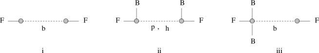
Figure 2: Two point amplitude upto quadratic order in $B$. (i) and (iii) are due to only $b$-field exchange, (ii) is due to graviton and dilaton exchange.

The propagators are the usual ones, rewriting them from eqns(4.2, 4.12,4.16),

$$<h_{ij}h_{i^{{}^{\prime}}j^{{}^{\prime}}}> = -2i\kappa^{2}\frac{[\eta_{ii^{{}^{\prime}}}\eta_{jj^{{}^{\prime}}}+\eta_{ij^{{}^{\prime}}}\eta_{i^{{}^{\prime}}j}-2/(D-2)\eta_{ij}\eta_{i^{{}^{\prime}}j^{{}^{\prime}}}]}{k_{\perp}^{2}+k_{\parallel}^{2}}$$ (4.26)

$$<\phi\phi> = -\frac{(D-2)i\kappa^{2}}{4}\frac{1}{k_{\perp}^{2}+k_{\parallel}^{2}}$$ (4.27)

$$<b_{ij}b_{i^{{}^{\prime}}j^{{}^{\prime}}}> = -\frac{2i\kappa^{2}}{(2\pi\alpha^{{}^{\prime}})^{2}}\frac{[\eta_{ii^{{}^{\prime}}}\eta_{jj^{{}^{\prime}}}-\eta_{ji^{{}^{\prime}}}\eta_{ij^{{}^{\prime}}}]}{k_{\perp}^{2}+k_{\parallel}^{2}}$$ (4.28)

With these, the contributions from the three modes to the two point function can be worked out. We are interested in the correction to the quadratic term in the effective action for the gauge field on the brane. This can be constructed with the vertices computed above and the propagators for the intermediate massless closed string states. This correction for the nonplanar diagram can be written as,

$$A_{2}(bb)=\int d^{p+1}\xi\int d^{p+1}\xi^{{}^{\prime}}b(\xi)b(\xi^{{}^{\prime}})V_{\chi}<\chi(\xi)\chi(\xi^{{}^{\prime}})>V_{\chi}$$ (4.29)

where,

$$<\chi(\xi)\chi(\xi^{{}^{\prime}})>=\int\frac{d^{D}k}{(2\pi)^{D}}<\chi(k_{\perp},k_{\parallel})\chi(-k_{\perp},-k_{\parallel})>e^{-ik_{\parallel}(\xi-\xi^{{}^{\prime}})}$$ (4.30)

We can rewrite eqn(4.29) in momentum space coordinates as,

$$A_{2}(bb) = {\cal V}_{p+1}\int\frac{d^{p+1}p}{(2\pi)^{p+1}}b(p)b(-p)\int\frac{d^{l}k_{\perp}}{(2\pi)^{l}}V_{\chi}<\chi(k_{\perp},-p)\chi(-k_{\perp},p)>V_{\chi}$$ (4.31)

$$= {\cal V}_{p+1}\int\frac{d^{p+1}p}{(2\pi)^{p+1}}b(p)b(-p)L_{2}(p,-p)$$

In the planar two point function, both the vertices are on the same end of the cylinder in the world-sheet computation. In the field theory this corresponds to putting both the vertices at the same position on the $D$-brane. In other words, in the expansion of the DBI action, we should be looking for $b^{2}\chi$ vertices on one end and a $\chi$ tadpole on the other. In this case, from the above calculation, $k_{\parallel}=0$. So the closed string propagator is just $1/k_{\perp}^{2}$, i.e. the propagator is not modified by the momentum of the gauge field on the brane. This is what we expect, as in the field theory on the brane, the loop integrals are not modified for the planar diagrams. Here we will only concentrate on the nonplanar sector.

As mentioned earlier, on the brane we will identify,

$$b_{kl}(p)\equiv\frac{g_{0}}{\sqrt{2\alpha^{{}^{\prime}}}}F_{kl}(p)=\frac{g_{0}}{\sqrt{2\alpha^{{}^{\prime}}}}p_{[k}A_{l]}(p)$$ (4.32)

The two point amplitude including the graviton, dilaton and $b$ field exchange is given by,

$$L_{2} = -i\kappa^{2}\tau_{p}^{2}\int\frac{d^{l}k_{\perp}}{(2\pi)^{l}}\frac{1}{k_{\perp}^{2}+p^{2}}\times$$

$$\times [(2\pi\alpha^{{}^{\prime}})^{4}\frac{D-2}{32}B^{kl}B^{k^{{}^{\prime}}l^{{}^{\prime}}}+\frac{(2\pi\alpha^{{}^{\prime}})^{2}}{4}\{1-\frac{(2\pi\alpha^{{}^{\prime}})^{2}}{2}\mbox{Tr}(B^{2})\}(\eta^{ll^{{}^{\prime}}}\eta^{kk^{{}^{\prime}}}-\eta^{lk^{{}^{\prime}}}\eta^{kl^{{}^{\prime}}})$$

$$+ \frac{(2\pi\alpha^{{}^{\prime}})^{4}}{2}\{(B^{2})^{kk^{{}^{\prime}}}\eta^{ll^{{}^{\prime}}}-(B^{2})^{kl^{{}^{\prime}}}\eta^{lk^{{}^{\prime}}}\}+(kl)\leftrightarrow(k^{{}^{\prime}}l^{{}^{\prime}})]$$

The full two point effective action, can now be constructed by putting back $L_{2}$ in eqn(4.31) along with the identification eqn(6.8). To compare this with the closed string channel result with only massless exchanges, eqn(3.16) we must note the expansions of the following quantities to appropriate powers of $B$.

$$G^{ij} \sim \eta^{ij}+(2\pi\alpha^{{}^{\prime}})^{2}(B^{2})^{ij}+{\cal O}(B^{4})$$ (4.34)

$$\theta^{ij} \sim -(2\pi\alpha^{{}^{\prime}})^{2}B^{ij}+{\cal O}(B^{3})$$

$$\sqrt{\eta+(2\pi\alpha^{{}^{\prime}})B} \sim \left[1-\frac{(2\pi\alpha^{{}^{\prime}})^{2}}{4}\mbox{Tr}(B^{2})+{\cal O}(B^{4})\right]$$

With these expansions, we can see that eqn(3.16) equals the sum of massless contributions, in eqn(4.1).

4.2 Noncommutative case $(g=\epsilon\eta)$

We now turn to the Seiberg Witten limit, (2.5) which gives rise to noncommutative field theory on the brane. Here again we will be interested in writing out the two point function eqn(3.16) in the closed string channel as a sum of the massless closed string modes. Due to the scaling of the closed string metric, unlike the earlier case, we will now expand all results in powers of the scale parameter for closed string metric, $\epsilon$. We begin by expanding the DBI action,

$${\cal L}=\sqrt{(2\pi\alpha^{{}^{\prime}})e^{-(P+Q)\phi}(B+b)}\left[1+\frac{1}{(2\pi\alpha^{{}^{\prime}})e^{-Q\phi}(B+b)}\epsilon(\eta+h)\right]^{1/2}$$ (4.35)

The $\phi$ and $b$-field vertices from this are,

$$V_{\phi}=\sqrt{(2\pi\alpha^{{}^{\prime}})B}\left[-\frac{1}{2}\left(\frac{1}{B}\right)^{kl}+\frac{\epsilon^{2}(4Q-2)}{4(2\pi\alpha^{{}^{\prime}})^{2}}\left(\left(\frac{1}{B^{3}}\right)^{kl}-\frac{1}{4}\mbox{Tr}\left(\frac{1}{B^{2}}\right)\left(\frac{1}{B}\right)^{kl}\right)\right]$$

$$V_{b}=\sqrt{(2\pi\alpha^{{}^{\prime}})B}\left[\frac{1}{4}\left(\frac{1}{B}\right)^{kl}\left(\frac{1}{B}\right)^{ji}-\frac{1}{2}\left(\frac{1}{B}\right)^{jl}\left(\frac{1}{B}\right)^{ki}\right]$$ (4.36)

Note that We are interested in the two point function only upto ${\cal O}(\epsilon^{2})$, hence we need not consider the graviton vertex. Also the $b$-field propagator has a $\epsilon^{2}$ factor (4.12). So, it is only necessary to compute the dilaton vertex upto ${\cal O}(\epsilon^{2})$.

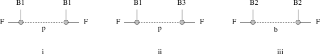
Figure 3: Two point amplitude upto ${\cal O}(\epsilon^{2})$. (i) and (ii) are due to dilaton exchange, (iii) is due to $b$-field exchange.

The exchanges with these couplings are summarised in Figure 3. The propagators in this limit, eqns(4.4,4.12),

$$<\phi\phi> = -\frac{(D-2)i\kappa^{2}}{4}\frac{1}{k_{\perp}^{2}+\epsilon^{-1}k_{\parallel}^{2}}$$ (4.37)

$$<b_{ij}b_{i^{{}^{\prime}}j^{{}^{\prime}}}> = -\frac{2i\kappa^{2}\epsilon^{2}}{(2\pi\alpha^{{}^{\prime}})^{2}}\frac{[\eta_{ii^{{}^{\prime}}}\eta_{jj^{{}^{\prime}}}-\eta_{ji^{{}^{\prime}}}\eta_{ij^{{}^{\prime}}}]}{k_{\perp}^{2}+\epsilon^{-1}k_{\parallel}^{2}}$$ (4.38)

With the vertices computed above and the propagator in this limit, the two point function is,

$$L_{2} = -i\mbox{det}(2\pi\alpha^{{}^{\prime}}B)\kappa^{2}\tau_{p}^{2}\int\frac{d^{l}k_{\perp}}{(2\pi)^{l}}\frac{1}{k_{\perp}^{2}+\epsilon^{-1}p^{2}}[{\cal O}(1)+{\cal O}(\epsilon^{2})]$$ (4.39)

where,

$${\cal O}(1)=\left[\frac{(D-2)}{32}\left(\frac{1}{B}\right)^{kl}\left(\frac{1}{B}\right)^{k^{{}^{\prime}}l^{{}^{\prime}}}+(kl)\leftrightarrow(k^{{}^{\prime}}l^{{}^{\prime}})\right]$$ (4.40)

$${\cal O}(\epsilon^{2}) = \frac{\epsilon^{2}}{(2\pi\alpha^{{}^{\prime}})^{2}}\frac{(D-2)}{16}\left[\left[\left(\frac{1}{B^{3}}\right)^{kl}-\frac{1}{4}\mbox{Tr}\left(\frac{1}{B^{2}}\right)\left(\frac{1}{B}\right)^{kl}\right]\left(\frac{1}{B}\right)^{k^{{}^{\prime}}l^{{}^{\prime}}}\right]$$ (4.41)

$$+ \frac{\epsilon^{2}}{(2\pi\alpha^{{}^{\prime}})^{2}}\left[\frac{1}{4}\left(\frac{1}{B^{2}}\right)^{kk^{{}^{\prime}}}\left(\frac{1}{B^{2}}\right)^{ll^{{}^{\prime}}}-\frac{1}{4}\left(\frac{1}{B^{2}}\right)^{k^{{}^{\prime}}l}\left(\frac{1}{B^{2}}\right)^{kl^{{}^{\prime}}}\right]$$

$$+ (kl)\leftrightarrow(k^{{}^{\prime}}l^{{}^{\prime}})$$

We can now reconstruct the quadratic term in effective action, (4.31) following the earlier case. With the following expansions, it is easy to check that the sum of the massless contributions adds upto eqn(3.16).

$$G^{ij} \sim -\frac{\epsilon}{(2\pi\alpha^{{}^{\prime}})^{2}}\left(\frac{1}{B^{2}}\right)^{ij}+{\cal O}(\epsilon^{3})$$ (4.42)

$$\theta^{ij} \sim \left(\frac{1}{B}\right)^{ij}+\frac{\epsilon^{2}}{(2\pi\alpha^{{}^{\prime}})^{2}}\left(\frac{1}{B^{3}}\right)^{ij}$$

$$\sqrt{\epsilon\eta+(2\pi\alpha^{{}^{\prime}})B} \sim \sqrt{(2\pi\alpha^{{}^{\prime}})B}\left[1-\frac{\epsilon^{2}}{4(2\pi\alpha^{{}^{\prime}})^{2}}\mbox{Tr}\left(\frac{1}{B^{2}}\right)\right]$$

Note that, at the tree-level, to the linear order, $\hat{F}=F$, (2.9). At this quadratic order in the effective action there is no need for redefinition of $F$ to equate the result here with that of string theory result in eqn(3.16).

4.3 Noncommutative case ($G=\eta$)

In this part we finally consider the restriction of the open string metric, $G=\eta$. The lowest order solution for the closed string metric, $g$ in $\alpha^{{}^{\prime}}$ in this limit is,

$$g=-(2\pi\alpha^{{}^{\prime}})^{2}B^{2}+{\cal O}(\alpha^{{}^{\prime}4})$$ (4.43)

We will now consider expansions of the two point functions in powers of $\alpha^{{}^{\prime}}$. We begin again with the following DBI Lagrangian,

$${\cal L} = \sqrt{(2\pi\alpha^{{}^{\prime}})e^{-(P+Q)\phi}(B+b)}\left[1-\frac{1}{e^{-Q\phi}(B+b)}(2\pi\alpha^{{}^{\prime}})B^{2}(\eta+h)^{2}\right]^{1/2}$$

The calculation for the vertices is same as before, there is no graviton vertex to the leading orders. The dilaton and the $b$-field vertices are,

$$V_{\phi}=\sqrt{(2\pi\alpha^{{}^{\prime}})B}\left[-\frac{1}{2}\left(\frac{1}{B}\right)^{kl}+\frac{(2\pi\alpha^{{}^{\prime}})^{2}(4Q-2)}{4}\left(B^{kl}-\frac{1}{4}\mbox{Tr}(B^{2})\left(\frac{1}{B}\right)^{kl}\right)\right]$$

$$V_{b}=\sqrt{(2\pi\alpha^{{}^{\prime}})B}\left[\frac{1}{4}\left(\frac{1}{B}\right)^{kl}\left(\frac{1}{B}\right)^{ji}-\frac{1}{2}\left(\frac{1}{B}\right)^{jl}\left(\frac{1}{B}\right)^{ki}\right]$$ (4.45)

The propagators for the dilaton and the $b$-field are modified as,

$$<\phi\phi> = -\frac{(D-2)i\kappa^{2}}{4}\frac{1}{k_{\perp}^{2}+\tilde{k_{\parallel}}^{2}/(2\pi\alpha^{{}^{\prime}})^{2}}$$ (4.46)

$$<b_{ij}b_{i^{{}^{\prime}}j^{{}^{\prime}}}> = -2i\kappa^{2}(2\pi\alpha^{{}^{\prime}})^{2}\frac{[B^{2}_{ii^{{}^{\prime}}}B^{2}_{jj^{{}^{\prime}}}-B^{2}_{ji^{{}^{\prime}}}B^{2}_{ij^{{}^{\prime}}}]}{k_{\perp}^{2}+\tilde{k_{\parallel}}^{2}/(2\pi\alpha^{{}^{\prime}})^{2}}$$ (4.47)

Figure 4: Two point amplitude upto ${\cal O}(\alpha^{{}^{\prime}2})$. (i) and (ii) are due to dilaton exchange, (iii) is due to $b$-field exchange.

With these vertices (shown in Figure 4) and the propagators from eqns(4.6,4.12), the two point function is now given by,

$$L_{2}=-i\det(2\pi\alpha^{{}^{\prime}}B)\kappa^{2}\tau_{p}^{2}\int\frac{d^{l}k_{\perp}}{(2\pi)^{l}}\frac{1}{k_{\perp}^{2}+\tilde{p}^{2}(2\pi\alpha^{{}^{\prime}})^{2}}[{\cal O}(1)+{\cal O}(\alpha^{{}^{\prime}2})]$$ (4.48)

$${\cal O}(1)=\left[\frac{(D-2)}{32}\left(\frac{1}{B}\right)^{kl}\left(\frac{1}{B}\right)^{k^{{}^{\prime}}l^{{}^{\prime}}}+(kl)\leftrightarrow(k^{{}^{\prime}}l^{{}^{\prime}})\right]$$ (4.49)

$${\cal O}(\alpha^{{}^{\prime}2}) = (2\pi\alpha^{{}^{\prime}})^{2}\frac{(D-2)}{16}\left[\left[B^{kl}-\frac{1}{4}\mbox{Tr}(B^{2})\left(\frac{1}{B}\right)^{kl}\right]\left(\frac{1}{B}\right)^{k^{{}^{\prime}}l^{{}^{\prime}}}\right]$$ (4.50)

$$+ (2\pi\alpha^{{}^{\prime}})^{2}\left[\frac{1}{4}\left(\eta^{ll^{{}^{\prime}}}\eta^{kk^{{}^{\prime}}}-\eta^{kl^{{}^{\prime}}}\eta^{lk^{{}^{\prime}}}\right)\right]$$

$$+ (kl)\leftrightarrow(k^{{}^{\prime}}l^{{}^{\prime}})$$

We will need the following expansions in this limit, to expand the closed string channel result upto this order. We have already set,

$$G^{ij} = \eta^{ij}$$ (4.51)

and with the solution for $g$, eqn(4.43) to the lowest order in $\alpha^{{}^{\prime}}$,

$$\theta^{ij} \sim \left(\frac{1}{B}\right)^{ij}+(2\pi\alpha^{{}^{\prime}})^{2}B^{ij}$$ (4.52)

$$\sqrt{g+(2\pi\alpha^{{}^{\prime}})B} \sim \sqrt{(2\pi\alpha^{{}^{\prime}})B}\left[1-\frac{(2\pi\alpha^{{}^{\prime}})^{2}}{4}\mbox{Tr}(B^{2})\right]$$ (4.53)

As in the earlier cases, the massless contributions computed here, eqn(4.48) adds upto eqn(3.16). Note that the situation here is similar to that of the earlier case in Section 4.2. As $\alpha^{{}^{\prime}}\sim\sqrt{\epsilon}$, the closed string metric in both the cases goes to zero as $g\sim\epsilon$. However the difference being that the two point amplitude differ by powers of $B$ in both the cases, due to the relative power of $B^{2}$ in $g$ in this case. Here too, the SW map between the usual and the noncommutative field strength eqn(2.9), remains the same. The differences in the powers of $B$ in the two point amplitudes, eqn(4.39) and eqn(4.48) are absorbed in $G$, $\theta$ and $\sqrt{g+(2\pi\alpha^{{}^{\prime}})B}$ in the two cases. We can work with any of the forms of the closed string metric $g$, the important point being that $g$ should go to zero as $\epsilon$ which gives the noncommutative gauge theory on the brane.

5 Open superstring in background $B$-field

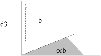
Figure 5: The background for string propagation. $D_{3}$ brane world volume directions are 0,1,2,3. Orbifolded directions 6,7,8,9.

After studying the bosonic case, let us now turn to the supersymmetric example. With the observations made in Section 3 we will consider ${\cal N}=2$ gauge theory that can be realised on a fractional $D_{3}$ brane located at the fixed point of $C^{2}/Z_{2}$ orbifold. The setup is shown in Figure 5. With the $B$-field turned on along the world-volume directions, the low-energy effective theory on the brane is described by a noncommutative ${\cal N}=2$ gauge theory. The world-sheet action for the fermions coupled to $B$-field is given by,

$$S_{F}=\frac{i}{4\pi\alpha^{{}^{\prime}}}\int_{\Sigma}g_{MN}\bar{\psi}^{M}\rho^{\alpha}\partial_{\alpha}\psi^{N}-\frac{i}{4}\int_{\partial\Sigma}B_{MN}\bar{\psi}^{N}\rho^{0}\psi^{M}$$ (5.1)

The full action including the bosons (2.1) and the fermions (5.1) with the bulk and the boundary terms are invariant under the following supersymmetry transformations,

$$\delta X^{M} = \bar{\epsilon}\psi^{M}$$

$$\delta\psi^{M} = -i\rho^{\alpha}\partial_{\alpha}X^{M}\epsilon$$ (5.2)

We now write down the boundary equations by varying (5.1) with the following constraints,

$$\delta\psi^{M}_{L}=\delta\psi^{M}_{R}\mid_{\sigma=\pi}\mbox{\hskip 14.45377ptand\hskip 14.45377pt}\delta\psi^{M}_{L}=-(-1)^{a}\delta\psi^{M}_{R}\mid_{\sigma=0}$$ (5.3)

where, $a=0,1$ gives the NS and the R sectors respectively This gives the following boundary equations,

$$g_{MN}(\psi_{L}^{N}-\psi_{R}^{N})+2\pi\alpha^{{}^{\prime}}B_{MN}(\psi_{L}^{N}+\psi_{R}^{N})=0\mid_{\sigma=\pi}$$ (5.4)

$$g_{MN}(\psi_{L}^{M}+(-1)^{a}\psi_{R}^{M})+2\pi\alpha^{{}^{\prime}}B_{MN}(\psi_{L}^{N}-(-1)^{a}\psi_{R}^{N})=0\mid_{\sigma=0}$$ (5.5)

To write down the correlator for the fermions, first define,

$$\psi^{M} = \psi^{M}_{L}(\sigma,\tau)\mbox{\hskip 36.135pt}0\leq\sigma\leq\pi$$ (5.6)

$$= \left(\frac{g-2\pi\alpha^{{}^{\prime}}B}{g+2\pi\alpha^{{}^{\prime}}B}\right)^{M}_{N}\psi_{R}^{N}(2\pi-\sigma,\tau)\mbox{\hskip 36.135pt}\pi\leq\sigma\leq 2\pi$$

This is the usual doubling trick that ensures the boundary conditions (5.4). In the following section we would compute the two point function for the gauge field on the brane by inserting two vertex operators at the boundaries of the cylinder. Restricting ourselves to the directions along the brane, this vertex operator for the gauge field in the zero picture is given by,

$$V(p,x,y)=\frac{g_{o}}{(2\alpha^{{}^{\prime}})^{1/2}}\epsilon_{j}\left(i\partial_{y}X^{j}+4p.\Psi\Psi^{j}\right)e^{ip.X}(x,y)$$ (5.7)

where $\Psi^{i}$ is given by,

$$\Psi^{i}(0,\tau) = \frac{1}{2}\left(\psi^{i}_{L}(0,\tau)+(-1)^{a+1}\psi^{i}_{R}(0,\tau)\right)=\left(\frac{1}{g-2\pi\alpha^{{}^{\prime}}B}g\right)^{i}_{j}\psi_{L}^{j}(0,\tau)$$

$$\Psi^{i}(\pi,\tau) = \frac{1}{2}\left(\psi^{i}_{L}(\pi,\tau)+\psi^{i}_{R}(\pi,\tau)\right)=\left(\frac{1}{g-2\pi\alpha^{{}^{\prime}}B}g\right)^{i}_{j}\psi_{L}^{j}(\pi,\tau)$$ (5.8)

Using (5), the correlation function for $\Psi$ is given by,

$$\left\langle\Psi^{i}(w)\Psi^{j}(w^{{}^{\prime}})\right\rangle=G^{ij}{\cal G}\left[\begin{smallmatrix}\alpha\\ \beta\end{smallmatrix}\right](w-w^{{}^{\prime}})$$ (5.9)

where $G^{ij}$ is the open string metric defined in (2) and, ${\cal G}\left[\begin{smallmatrix}\alpha\\ \beta\end{smallmatrix}\right](w-w^{{}^{\prime}})$ is given by [44],

$${\cal G}\left[\begin{smallmatrix}\alpha\\ \beta\end{smallmatrix}\right](w-w^{{}^{\prime}})=\frac{\alpha^{{}^{\prime}}}{4\pi}\frac{\vartheta\left[\begin{smallmatrix}\alpha\\ \beta\end{smallmatrix}\right]\left(\frac{w-w^{{}^{\prime}}}{2\pi},it\right)\vartheta^{{}^{\prime}}\left[\begin{smallmatrix}1/2\\ 1/2\end{smallmatrix}\right](0,it)}{\vartheta\left[\begin{smallmatrix}1/2\\ 1/2\end{smallmatrix}\right]\left(\frac{w-w^{{}^{\prime}}}{2\pi},it\right)\vartheta\left[\begin{smallmatrix}\alpha\\ \beta\end{smallmatrix}\right](0,it)}$$ (5.10)

$\alpha,\beta$ denotes the spin structures. $\alpha=(0,1/2)$ are the NS and the R sectors and $\beta=(0,1/2)$ stands for the absence or the presence of the world-sheet fermion number $(-1)^{F}$ with $\psi$ being anti-periodic or periodic along the $\tau$ direction on the world-sheet. $w$, $w^{{}^{\prime}}$ are located at the boundaries of the world-sheet for the open string which is a cylinder, i.e. at $\sigma=0,\pi$.

5.1 Strings on $C^{2}/Z_{2}$ orbifold

An efficient and simple way to break ${\cal N}=4$ supersymmetry and obtain gauge theories with less supersymmetries is by orbifolding the background space. Specifically strings on $C^{2}/Z_{2}$ gives rise to ${\cal N}=2$ supersymmetric gauge theory on D3-branes with world volume directions transverse to the Orbifolded planes. The open and the closed string spectrum on this orbifold have been nicely worked out in [40]. We include a brief analysis here that will be relevant in the later discussions. We will take the orbifolded directions to be $6,7,8,9$ with $Z_{2}=\{g_{i}\mid e,g\}$ such that $g^{2}=e$ The action of $g$ on these coordinates is given by,

$$gX^{I}=-X^{I}\mbox{\hskip 36.135pt for \hskip 36.135pt}I=6,7,8,9$$ (5.11)

In order to preserve world sheet supersymmetry we must also consider the action of $Z_{2}$ on the fermionic partners, $\psi^{I}$.

5.1.1 Open string spectrum and fractional branes

On a particular state of the open string the orbifold action is on the oscillators, $\psi^{I}_{-r}$ along with the Chan-Paton indices associated with it. Let us consider the massless bosonic states from the NS sector.

$$g|i,j,\psi^{I}_{-1/2}>=\gamma_{ii^{{}^{\prime}}}|i^{{}^{\prime}},j^{{}^{\prime}},\hat{g}\psi^{I}_{-1/2}>\gamma^{-1}_{j^{{}^{\prime}}j}$$ (5.12)

where $\gamma$ is a representation of $Z_{2}$ The spectrum is obtained by keeping the states that are invariant under the above action. To derive this it is easier to work in the basis where $\gamma$ is diagonal,

$$\gamma=\sigma_{3}=\left(\begin{matrix}1&0\\ 0&-1\end{matrix}\right)$$ (5.13)

The action on the Chan-Paton indices can be thought of as,

$$\gamma\left(\begin{matrix}11&12\\ 21&22\end{matrix}\right)\gamma^{-1}=\left(\begin{matrix}11&-12\\ -21&22\end{matrix}\right)$$ (5.14)

Thus the diagonal ones survive for the $Z_{2}$ action on the oscillators is $\hat{g}|\psi^{I}_{-1/2}>=|\psi^{I}_{-1/2}>$, i,e. for $I=2,3,4,5$ and the off-diagonal ones are preserved for oscillators that are odd under the $Z_{2}$ action, $\hat{g}|\psi^{I}_{-1/2}>=-|\psi^{I}_{-1/2}>$, i,e. for $I=6,7,8,9$. The spectrum can thus be summarised as,

$$A^{I}\rightarrow\left[\begin{matrix}A^{I}_{1}&A^{I}_{2}&\mbox{$2$ gauge fields}&I=2,3\\ \phi^{I}_{1}&\phi^{I}_{2}&\mbox{$4$ real scalars}&I=4,5\\ \Phi^{I}_{1}&\Phi^{I}_{2}&\mbox{$8$ real scalars}&I=6,7,8,9\\ \end{matrix}\right]$$ (5.15)

The orbifold action on the space-time spinors is given by,

$$\chi_{ij}\rightarrow\gamma_{ii^{{}^{\prime}}}e^{i\pi(s_{3}+s_{4})}\chi_{i^{{}^{\prime}}j^{{}^{\prime}}}\gamma_{j^{{}^{\prime}}j}^{-1}$$ (5.16)

where $\chi_{i^{{}^{\prime}}j^{{}^{\prime}}}=\left|s_{1},s_{2},s_{3},s_{4}\right\rangle_{i^{{}^{\prime}}j^{{}^{\prime}}}$ are the sixteen spinors of $SO(8)$, with $s_{i}=\pm 1/2$. The spinors in (5.16) are left invariant for, $s_{3}+s_{4}=0$ and $s_{3}+s_{4}=\pm 1$. The first one leaves $\chi_{11}$ and $\chi_{22}$ invariant and the second one leaves $\chi_{12}$ and $\chi_{21}$. Projection onto one of the chiralities leaves four copies of each of the spinors.

The above fields can be grouped into two vector multiplets and two hypermultiplets of ${\cal N}=2$ with gauge group $U(1)\times U(1)$. The beta function for the gauge couplings for this theory vanishes and the theory is conformally invariant. Now consider an irreducible representation $\gamma=\pm 1$. This acts trivially on the Chan-Paton indices. These branes are known as fractional branes. From the geometric point of view there is no image for the $D3$ brane. The brane is localised at the fixed point on the orbifold plane but is free to move in the non-orbifolded (4,5) directions.

Following the above analysis, the spectrum consists of a single gauge field and two scalars completing the vector multiplet of ${\cal N}=2$ with gauge group $U(1)$. The beta function for this theory is nonzero. With a constant $B$-field turned on along the world volume directions of the $D_{3}$-brane,$(0,1,2,3)$, the low energy dynamics on the brane will be described be noncommutative gauge theory in the Seiberg-Witten limit. In the following section we will study the ultraviolet behaviour of this theory and see how the UV divergences have a natural interpretation in terms of IR divergences due to massless closed string modes as a result of open-closed string duality.

5.1.2 Closed string spectrum

The closed string theory consists of additional twisted sectors apart from the untwisted sectors. The orbifold action on the space-time implies the following boundary conditions on the world-sheet bosons and fermions,

$$X^{I}(\sigma+2\pi,\tau) = \pm X^{I}(\sigma,\tau)$$

$$\psi^{I}(\sigma+2\pi,\tau) = \pm\psi^{I}(\sigma,\tau)\mbox{\hskip 14.45377pt}I=6,7,8,9$$ (5.17)

For the world sheet fermions, the $(+)$-sign stands for the NS-sector and the $(-)$-sign for the R-sector. For the other directions the boundary conditions on the world-sheet fields are as usual. We will first list the fields in the untwisted sectors. In the NS-NS sector the massless states invariant under the orbifold projection are,

$$\psi_{-1/2}^{I}\tilde{\psi}_{-1/2}^{J}\left|0,k\right\rangle$$ (5.18)

where, $I,J=\{2,3,4,5\}$ or $I,J=\{6,7,8,9$}. The first set of oscillators give the graviton, antisymmetric 2-form field, and the dilaton. The second set gives sixteen scalars.

The orbifold action on the spinor of $SO(8)$ is given by,

$$\left|s_{1},s_{2},s_{3},s_{4}\right\rangle\rightarrow e^{i\pi(s_{3}+s_{4})}\left|s_{1},s_{2},s_{3},s_{4}\right\rangle$$ (5.19)

The $Z_{2}$ invariant R-R state is formed by taking both the left the right states to be either even or odd under $Z_{2}$ projection corresponding to $s_{3}+s_{4}=0$ or $s_{3}+s_{4}=\pm 1$ respectively. GSO projection, restricting to both the left and right states to be of the same chirality gives thirty two states. These states correspond to four 2-form fields and eight scalars.

Let us now turn to the twisted sectors. For the twisted sectors the ground state energy for both the NS and the R sectors vanish. In the NS sector the massless modes come from $\psi^{I}_{0}$, $I=6,7,8,9$ oscillators which form a spinor representation of $SO(4)$. With the GSO and the orbifold projections, the closed string spectrum is given by, $2\times 2=[0]+[2]$. The [0] and the self-dual [2] constitute the four massless scalars in the NS-NS sector. Similarly, in the R sector, the massless modes are given by $\psi^{I}_{0}$ for $I=2,3,4,5$. Thus giving a scalar and a two-form self-dual field in the closed string R-R sector. The couplings for the massless closed string states to the fractional $D_{3}$-brane will be studied in Sections 7.2.1 and 7.2.2.

6 Open string one loop amplitude : IIB on $C^{2}/Z_{2}$

In this section we compute the two point function for the gauge fields on the brane. The necessary ingredients are given in Section 5 and in the Appendix A. The one loop vacuum amplitude vanishes as a result of supersymmetry, i.e.

$$\det(g+2\pi\alpha^{{}^{\prime}}B)\int^{\infty}_{0}\frac{dt}{4t}(8\pi^{2}\alpha^{{}^{\prime}}t)^{-2}\sum_{(\alpha,\beta,g_{i})}Z\left[\begin{smallmatrix}\alpha\\ \beta\end{smallmatrix}\right]_{g_{i}}=0$$ (6.1)

The factor of $\det(g+2\pi\alpha^{{}^{\prime}}B)$ comes from the trace over the world sheet bosonic zero modes. The sum is over the spin structures $(\alpha,\beta)=(0,1/2)$ corresponding to the NS and R sectors and the GSO projection and the orbifold projection. The elements $Z_{g_{i}}{\left[\begin{smallmatrix}\alpha\\ \beta\end{smallmatrix}\right]}$ are computed in the Appendix A. Let us now compute the two point function. This is given by,

$$A(p,-p) = \det(g+2\pi\alpha^{{}^{\prime}}B)\int^{\infty}_{0}\frac{dt}{4t}(8\pi^{2}\alpha^{{}^{\prime}}t)^{-2}\times$$

$$\times \sum_{(\alpha,\beta,g_{i})}Z{\left[\begin{smallmatrix}\alpha\\ \beta\end{smallmatrix}\right]}_{g_{i}}\int_{0}^{2\pi t}dy\int_{0}^{2\pi t}dy^{{}^{\prime}}\left\langle V(p,x,y)V(-p,x^{{}^{\prime}},y^{{}^{\prime}})\right\rangle_{(\alpha,\beta)}$$

For the flat space, it is well known that amplitudes with less that four boson insertions vanish. However, in this model the two point amplitude survives. We will now compute this amplitude in the presence of background $B$-field. First note that the bosonic correlation function, $\left\langle:\partial_{y}X^{i}e^{ip.X}::\partial_{y}^{{}^{\prime}}X^{i}e^{-ip.X}:\right\rangle$, does not contribute to the two point amplitude as it is independent of the spin structure. The two point function would involve the sum over the $Z_{g_{i}}\left[\begin{smallmatrix}\alpha\\ \beta\end{smallmatrix}\right]$ which makes this contribution zero due to (6.1). The nonzero part of the amplitude will be obtained from the fermionic part,

$$\epsilon_{k}\epsilon_{l}\left\langle:p.\Psi\Psi^{k}e^{ip.X}::p.\Psi\Psi^{l}e^{-ip.X}:\right\rangle = \epsilon_{k}\epsilon_{l}p_{i}p_{j}\left(G^{il}G^{jk}-G^{ij}G^{kl}\right)\times$$

$$\times {\cal G}^{2}\left[\begin{smallmatrix}\alpha\\ \beta\end{smallmatrix}\right](w-w^{{}^{\prime}})\left\langle:e^{ip.X}::e^{-ip.X}:\right\rangle$$

For the planar two point amplitude, both the vertex operators would be inserted at the same end of the cylinder (i.e. at $w=0+iy$ or $\pi+iy$). In this case, the sum in the two point amplitude reduces to,

$$\sum_{(\alpha,\beta,g_{i})}Z\left[\begin{smallmatrix}\alpha\\ \beta\end{smallmatrix}\right]_{g_{i}}{\cal G}^{2}\left[\begin{smallmatrix}\alpha\\ \beta\end{smallmatrix}\right](i\Delta y/2\pi) = \sum_{(\alpha,\beta)}Z\left[\begin{smallmatrix}\alpha\\ \beta\end{smallmatrix}\right]_{e}{\cal G}^{2}\left[\begin{smallmatrix}\alpha\\ \beta\end{smallmatrix}\right](i\Delta y/2\pi)$$

$$+ \sum_{(\alpha,\beta)}Z\left[\begin{smallmatrix}\alpha\\ \beta\end{smallmatrix}\right]_{g}{\cal G}^{2}\left[\begin{smallmatrix}\alpha\\ \beta\end{smallmatrix}\right](i\Delta y/2\pi)$$

$$= \frac{4\pi^{2}}{\eta(it)^{6}\vartheta^{2}_{1}(i\Delta y/2\pi,it)}\sum_{(\alpha,\beta)}\vartheta^{2}\left[\begin{smallmatrix}\alpha\\ \beta\end{smallmatrix}\right](0,it)\vartheta^{2}\left[\begin{smallmatrix}\alpha\\ \beta\end{smallmatrix}\right](i\Delta y/2\pi,it)+$$

$$+ \frac{16\pi^{2}}{\vartheta^{2}_{1}(i\Delta y/2\pi,it)\vartheta^{2}_{2}(0,it)}\left[\vartheta^{2}_{3}(i\Delta y/2\pi,it)\vartheta^{2}_{4}(0,it)-\vartheta^{2}_{4}(i\Delta y/2\pi,it)\vartheta^{2}_{3}(0,it)\right]$$

where, $\Delta y=y-y^{{}^{\prime}}$. We have separated the total sum as the sum over the two $Z_{2}$ group actions. In writing this we have used the following identity

$$\eta(it)=\left[\frac{\partial_{\nu}\vartheta_{1}(\nu,it)}{-2\pi}\right]^{1/3}_{\nu=0}$$ (6.5)

Now, the first term vanishes due to the following identity

$$\sum_{(\alpha,\beta)}\vartheta\left[\begin{smallmatrix}\alpha\\ \beta\end{smallmatrix}\right](u)\vartheta\left[\begin{smallmatrix}\alpha\\ \beta\end{smallmatrix}\right](v)\vartheta\left[\begin{smallmatrix}\alpha\\ \beta\end{smallmatrix}\right](w)\vartheta\left[\begin{smallmatrix}\alpha\\ \beta\end{smallmatrix}\right](s)=$$

$$2\vartheta\left[\begin{smallmatrix}1/2\\ 1/2\end{smallmatrix}\right](u_{1})\vartheta\left[\begin{smallmatrix}1/2\\ 1/2\end{smallmatrix}\right](v_{1})\vartheta\left[\begin{smallmatrix}1/2\\ 1/2\end{smallmatrix}\right](w_{1})\vartheta\left[\begin{smallmatrix}1/2\\ 1/2\end{smallmatrix}\right](s_{1})$$

where,

$$u_{1} = \frac{1}{2}(u+v+w+s)\mbox{\hskip 14.45377pt}v_{1}=\frac{1}{2}(u+v-w-s)\mbox{\hskip 14.45377pt}$$

$$w_{1} = \frac{1}{2}(u-v+w-s)\mbox{\hskip 14.45377pt}s_{1}=\frac{1}{2}(u-v-w+s)$$ (6.7)

and noting that, $\vartheta\left[\begin{smallmatrix}1/2\\ 1/2\end{smallmatrix}\right](0,it)=0$, in the same way as the flat case that makes amplitudes with two vertex insertions vanish. The second term is a constant also due to,

$$\vartheta^{2}_{4}(z,it)\vartheta^{2}_{3}(0,it)-\vartheta^{2}_{3}(z,it)\vartheta^{2}_{4}(0,it)=\vartheta^{2}_{1}(z,it)\vartheta^{2}_{2}(0,it)$$ (6.8)

For the nonplanar amplitude, that we are ultimately interested in, we need to put the two vertices at the two ends of the cylinder such that, $w=\pi+iy$ and $w^{{}^{\prime}}=iy^{{}^{\prime}}$. It can be seen that the fermionic part of the correlator is constant and independent of $t$, same as the planar case following from the identity (6.8). The effect of nonplanarity and the regulation of the two point function due to the background $B$-field is encoded in the correlation functions for the exponentials. The two point function thus reduces to,

$$A(p,-p)\sim\epsilon_{k}\epsilon_{l}p_{i}p_{j}\left(G^{il}G^{jk}-G^{ij}G^{kl}\right)\int^{\infty}_{0}\frac{dt}{4t}(8\pi^{2}\alpha^{{}^{\prime}}t)^{-2}\int_{0}^{2\pi t}dydy^{{}^{\prime}}\left\langle e^{ip.X}e^{-ip.X}\right\rangle$$

The noncommutative gauge theory two point function is obtained in the limit $t\rightarrow\infty$ and $\alpha^{{}^{\prime}}\rightarrow 0$. The correlation function in this limit can be computed from the bosonic correlation functions [26, 27, 28, 30, 45]. For the nonplanar case in this limit,

$$\left\langle e^{ip.X}e^{-ip.X}\right\rangle = \exp\left\{-p^{2}t\Delta x(\Delta x-1)-\frac{1}{4t}p_{i}(g^{-1}-G^{-1})^{ij}p_{j}\right\}$$ (6.10)

$$= \exp\left\{-p^{2}t\Delta x(\Delta x-1)-\frac{\tilde{p}^{2}}{4t}\right\}$$

where, $\tilde{p}=(\theta p)$. We have redefined the world sheet coordinate as $\Delta x=\Delta y/(2\pi t)$ and have scaled $t\rightarrow t/(2\pi\alpha^{{}^{\prime}})$. We have also used the following relation in writing down the last expression.

$$g^{-1}=G^{-1}-\frac{(\theta G\theta)}{(2\pi\alpha^{{}^{\prime}})^{2}}$$ (6.11)

The first term in the exponential in (6.10) regulates the integral over $t$ in the infrared, for $p\neq 0$ and the second term regulates it in the ultraviolet that is usually observed in noncommutative field theories. The $t\rightarrow\infty$ limit suppresses the contributions from all the open string massive modes. However as, discussed in Section 3, the field theory divergences still come from the $t\rightarrow 0$ region. We can thus break the integral over $t$ into two intervals $1/\Lambda^{2}\alpha^{{}^{\prime}}<t<\infty$ and $0<t<1/\Lambda^{2}\alpha^{{}^{\prime}}$ (see Figure 1). The second interval which is the source of the UV divergence is also the regime dominated by massless closed string exchanges. We now evaluate the two point function in this limit. First, the correlation function for the exponential in the $t\rightarrow 0$ limit is given by

$$\left\langle e^{ip.X}e^{-ip.X}\right\rangle=\exp\left\{-\frac{\alpha^{{}^{\prime}}\pi}{2t}p_{i}g^{ij}p_{j}\right\}$$ (6.12)

where $g^{ij}$ is the closed string metric. Modular transformation , ($t\rightarrow 1/t$) allows us to rewrite the one loop amplitude as the sum over closed string modes in a tree diagram. In the limit $t\rightarrow 0$, the amplitude will be dominated by massless closed string modes. In this model however, the effect of the massive modes in the loop cancel amongst themselves for any value of $t$. In the open string channel the $t\rightarrow 0$ limit would usually be contributed by the full tower of open string modes. However since we have seen that the effect of the massive string modes cancel anyhow for all values of $t$, the contribution to this limit from the open string modes comes only from the massless ones. The additional term in (6.10) as compared to (6.12) gives finite derivative corrections to the effective action. These would in general require the massive closed string states for its dual description. Without these derivative corrections, the contributions from the massless open string loop and the massless closed string tree are exactly equal. The divergent ultraviolet behaviour of the massless open string modes can thus be captured by the the massless closed string modes that have momentum in the limit $[0,1/\Lambda\alpha^{{}^{\prime}}]$. The amplitude can now be written as,

$$A(p,-p)={\cal V}_{4}\det(g+2\pi\alpha^{{}^{\prime}}B)\left(\frac{g_{o}^{2}}{8\pi^{2}\alpha^{{}^{\prime}}}\right)\epsilon_{k}\epsilon_{l}p_{i}p_{j}\left(G^{il}G^{jk}-G^{ij}G^{kl}\right)I(p)$$

where,

$$I(p) = \int dss^{-1}\exp\left\{-\frac{\alpha^{{}^{\prime}}\pi s}{2}p_{i}g^{ij}p_{j}\right\}$$ (6.14)

$$= 4\pi\int\frac{d^{2}k_{\perp}}{(2\pi)^{2}}\frac{1}{k_{\perp}^{2}+p_{i}g^{ij}p_{j}}$$

The integral is written in terms of $s=1/t$ and in the last line we have rewritten it as an integral over $k_{\perp}$, the momentum in the directions transverse to the brane for closed strings. The nonzero contribution to the two point amplitude in (6) comes from the $\mbox{Tr}_{NS}\left[gq^{L_{0}}\right]$ and $\mbox{Tr}_{NS}\left[g(-1)^{F}q^{L_{0}}\right]$, that are evaluated in (A.39). These correspond to anti-periodic NS-NS and periodic (R-R) closed strings in the twisted sectors respectively. The fractional $D_{3}$-brane is localised at the fixed point of $C^{2}/Z_{2}$. Thus the twisted sector closed string states that couple to it are twisted in all the directions of the orbifold. These modes are localised at the fixed point and are free to move in the six directions transverse to the orbifold. This is the origin of the momentum integral (6.14) in two directions transverse to the $D$-brane. These twisted states come from both the NS-NS and the R-R sectors and are listed in Section 5.1.2.

As we are interested in seeing the ultraviolet effect of the open string channel as an infrared effect in the closed string channel, like in the bosonic case (see eqn.(3.13)), we must cut off the $s$ integral at the lower end at some value $\Lambda^{2}\alpha^{{}^{\prime}}$ corresponding to the UV cut-off for the momentum of the massless closed strings in the directions transverse to the brane. With this, we have,

$$I(p,\Lambda)=4\pi^{2}\ln\left(\frac{p_{i}g^{ij}p_{j}+1/(\Lambda\alpha^{{}^{\prime}})^{2}}{p_{i}g^{ij}p_{j}}\right)$$ (6.15)

This is the ultraviolet behaviour of the two point function for two gauge fields in ${\cal N}=2$ theory. For the noncommutative theory it is regulated for $p\neq 0$. The fact that we are able to rewrite the gauge theory two point function as massless closed string tree-level exchanges is very specific to the ${\cal N}=2$ theory. The computations above show that the origin of this can be traced to open-closed string duality where the orbifold background cancels all contributions from the massive states as far as the UV singular terms are concerned. The background $B$-field in the SW limit only acts as a physical regulator.

7 Massless closed string exchanges

Let us now study in detail the massless closed string exchanges as in Section 4 that is discussed in more detail in [34]. The computation will be done for the three cases enumerated at the begining of this section. We will calculate the contribution to the nonplanar two point function with two gauge fields on the brane with massless closed string exchanges coming from the NS-NS and the R-R sectors. First we study the flat 10D case and then we will move on to the exchanges in the $C^{2}/Z_{2}$ orbifold background.

7.1 Type IIB on flat space

In this section we will consider the flat 10D case and consider massless closed string exchanges for a $D_{3}$ brane. The two point function will be shown to vanish as expected from the analysis in the previous section. See eqn(6). The results here will be necessary for the later part of this section when we study the exchanges on $C^{2}/Z_{2}$ orbifold. These will precisely be the contributions from the untwisted states upto an overall constant. To begin we write down the supergravity action for the type IIB theory in the Einstein frame

$$S_{IIB} = \frac{1}{2\kappa^{2}}\left[\int d^{10}x\sqrt{-g}R-\frac{1}{2}\int\left[d\phi\wedge*d\phi+e^{-\phi}H_{3}\wedge*H_{3}\right]\right]$$ (7.1)

$$- \frac{1}{4\kappa_{10}^{2}}\left[\int e^{2\phi}F_{1}\wedge*F_{1}+e^{\phi}F_{3}\wedge*F_{3}+\frac{1}{2}F_{5}\wedge*F_{5}\right]+...$$

where $\kappa^{2}=\kappa^{2}_{10}e^{-2\phi_{0}}$, and

$$H_{3}=db\mbox{\hskip 14.45377pt}F_{1}=dC_{0}\mbox{\hskip 14.45377pt}F_{3}=dC_{2}\mbox{\hskip 14.45377pt}F_{5}=dC_{4}$$ (7.2)

Where $b$ is the two form antisymmetric NS-NS field . We have omitted the other terms in the action (7.1) as we are only interested in the propagators for the closed string modes that will be needed to compute the two point amplitude in the later part of this section. The propagators for the NS-NS modes that have already been worked out in Section 4 in the context of bosonic string theory.

The R-R modes that will be relevant for our discussions are the zero-form, $C_{0}$ and the two-form, $C_{2}$. For the R-R modes, the propagators are same as that of the NS-NS modes upto normalisations,

$$\left\langle C_{0}C_{0}\right\rangle = \frac{\kappa_{10}^{2}}{\kappa^{2}}\left\langle\phi\phi\right\rangle$$

$$\left\langle C_{2IJ}C_{2I^{{}^{\prime}}J^{{}^{\prime}}}\right\rangle = \frac{\kappa_{10}^{2}}{\kappa^{2}}(2\pi\alpha^{{}^{\prime}})^{2}\left\langle b_{IJ}b_{I^{{}^{\prime}}J{{}^{\prime}}}\right\rangle$$ (7.3)

The propagators will be restricted to the values for the closed string metric $g^{ij}$ in the various limits stated at thebegining of this section. The correction to the quadratic term due to the tree-level closed string exchanges will be obtained as shown in eqn(4.31).

7.1.1 NS-NS exchange

We now turn to the DBI and the Chern-Simons action of a $D_{3}$ brane for calculating the massless closed string couplings to the gauge field The NS-NS field content is same as that of the bosonic theory. To compute the amplitude due to the exchange of these fields we need to set $D\rightarrow 10$ in the amplitudes calculated in Sections 4.1, 4.2 and 4.3 in equations (4.1),(4.39) and (4.48) respectively.

7.1.2 R-R exchange

The couplings of the R-R modes to the gauge field on the brane will be given by the usual Chern-Simons terms. We will consider here the commutative description of these terms. For a discussion of noncommutative description see [47, 48]

$$S_{CS}=i\mu_{3}\int_{4}\sum_{n}C_{n}\wedge e^{2\pi\alpha^{{}^{\prime}}(B+b)}$$ (7.4)

Expanding (7.4) and picking out the forms proportional to the volume form with one $b$ insertion we get

$$S_{CS}=i\mu_{3}\left[(2\pi\alpha^{{}^{\prime}})^{2}\int_{4}C_{0}B\wedge b+(2\pi\alpha^{{}^{\prime}})\int_{4}C_{2}\wedge b\right]$$ (7.5)

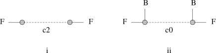
Figure 6: Two point amplitude upto quadratic order in $B$. (i) is due to $C_{2}$ exchange (ii) due to $C_{0}$ exchange.

$C_{2}$ Exchange :

The coupling of $C_{2}$ to $b$ is given by,

$$V_{bC_{2}}=\frac{i\mu_{3}}{4}(2\pi\alpha^{{}^{\prime}})\epsilon^{ijkl}$$ (7.6)

The two point amplitude can be worked out as in (4.31). For the noncommutative cases, we will rewrite the coupling (7.6) as

$$V_{bC_{2}}=\sqrt{2\pi\alpha^{{}^{\prime}}B}\frac{i\mu_{3}}{32(2\pi\alpha^{{}^{\prime}})}\left(\frac{1}{B}\right)^{pq}\left(\frac{1}{B}\right)^{rs}\epsilon_{pqrs}\epsilon^{ijkl}$$

$$=\sqrt{2\pi\alpha^{{}^{\prime}}B}\frac{i\mu_{3}}{4(2\pi\alpha^{{}^{\prime}})}\left[\left(\frac{1}{B}\right)^{ik}\left(\frac{1}{B}\right)^{jl}-\left(\frac{1}{B}\right)^{jk}\left(\frac{1}{B}\right)^{il}-\left(\frac{1}{B}\right)^{ij}\left(\frac{1}{B}\right)^{kl}\right]$$

Where we have used the fact that, for an antisymmetric matrix $M$ of rank $2n$, $\sqrt{M}=\frac{(-1)^{n}}{2^{n}n!}\epsilon_{\mu_{1}..\mu_{2n}}M^{\mu_{1}\mu_{2}}...M^{\mu_{2n-1}\mu_{2n}}$. The two point function can now be calculated with the above vertices. Note that the dependence of the amplitude on the closed string metric $g$ only comes from the propagator.

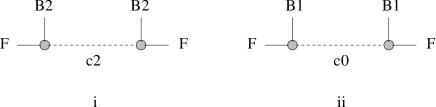
Figure 7: Two point amplitude upto ${\cal O}(\epsilon^{2})$ and ${\cal O}(\alpha^{{}^{\prime}2})$ . (i) is due to $C_{2}$ exchange (ii) due to $C_{0}$ exchange.

$C_{0}$ Exchange :

Reading from (7.5) the coupling of $C_{0}$ to the gauge field on the brane is given by

$$V_{bC_{0}}=\frac{i\mu_{3}}{4}(2\pi\alpha^{{}^{\prime}})^{2}B_{ij}\epsilon^{ijkl}$$ (7.8)

The noncommutative couplings can be obtained as the $C_{2}$ case, and finally contracting the answer with $B_{ij}$. This gives

$$V_{bC_{0}}=\sqrt{2\pi\alpha^{{}^{\prime}}B}\frac{i\mu_{3}}{2}\left(\frac{1}{B}\right)^{kl}$$ (7.9)

The $C_{2}$ and $C_{0}$ exchanges have been summarised for various limits of $g$ in Figures 6 and 7. For details of calculation see [34]. One can easily show that, with the identification $\kappa_{10}\mu_{3}=\kappa\tau_{3}$, the full contribution to the two point function including both the massless NS-NS exchanges in Section 4, and R-R exchanges considered here, vanishes. We know from the one loop string calculation that the one loop two point amplitude vanishes for the flat space background, (6) . In the closed string picture, this cancellation takes place for every mass-level between the NS-NS and R-R states. We will consider similar exchanges for the massless closed strings on the $C^{2}/Z_{2}$ orbifold in the next section.

7.2 Type IIB on $C^{2}/Z_{2}$ orbifold

In this section we analyse the closed string exchanges on the orbifold that we are ultimately interested in. The procedure followed is same as that of the earlier section. We will first write down the supergravity action on the $C^{2}/Z_{2}$ orbifold. We then derive the couplings of the massless closed string modes to the gauge field on a fractional $D_{3}$. We shall primarily make use of the fact that the $Z_{2}$ orbifold is the singular limit of a smooth ALE space known as Eguchi-Hanson space (See Appendix B). The orbifold singulatity arises as the radius of the compact 2-sphere reduces to zero size. The compact 2-sphere (${\cal C}_{1}$) has an associated antiself-dual two form, $\omega_{2}$ (B.4) that is dual to ${\cal C}_{1}$ and satisfies,

$$\omega_{2}=-*\omega_{2}\mbox{\hskip 14.45377pt}\int_{{\cal C}_{1}}\omega_{2}=1\mbox{\hskip 14.45377pt}\int_{C^{2}/Z_{2}}*\omega_{2}\wedge\omega_{2}=\frac{1}{2}$$ (7.10)

Although the cycle ${\cal C}_{1}$ shrinks to zero size, there is a non-zero two-form flux $\hat{B}$. A ($p+2$)-form may be dimensionally reduced as follows, $A_{p+2}=\tilde{A}_{p}\wedge\omega_{2}$. Where $\tilde{A}_{p}$ is a $p$-form in the transverse six dimensions. This field is twisted and is localised at the orbifold point. For the problem at hand we also turn on the ($B+b$) field along the non-orbifolded directions, so that the background is given by

$${\cal B}=\left(\begin{tabular}[]{cccc|ccl}0&1&2&3&...&8&9\\ &&&&&\\ &&$2\pi\alpha^{{}^{\prime}}(B+b)$&&&&\\ &&&&&&\\ \hline\cr&&&&&&\\ &&&&&&$\hat{B}$\\ \end{tabular}\right)$$ (7.17)

With the above observations and using equations (7.10), we can now write down the supergravity action on the orbifold for the twisted fields,

$$S_{orb}=-\frac{1}{8\kappa^{2}}\int_{6}d\tilde{b}\wedge*d\tilde{b}-\frac{1}{8\kappa_{10}^{2}}\int_{6}\left[d\tilde{C_{0}}\wedge*d\tilde{C_{0}}+d\tilde{C_{2}}\wedge*d\tilde{C_{2}}\right]$$ (7.18)

Where $\tilde{b}$ is the twisted NS-NS scalar that arises from the dimensional reduction of the $\hat{B}$ so that $\hat{B}=\hat{b}\omega_{2}$ and,

$$\hat{b}=4\pi^{2}\alpha^{{}^{\prime}}\left(\frac{1}{2}+\frac{\tilde{b}}{4\pi^{2}\alpha^{{}^{\prime}}}\right)$$ (7.19)

$\tilde{b}$ is the fluctuating part of $\hat{b}$. Similarly the scalar, $\tilde{C}_{0}$ and the two-form field $\tilde{C}_{2}$ arises from the dimensional reduction of the R-R fields $C_{2}$ and $C_{4}$ respectively. The propagators for these twisted fields can be easily read off from (7.18),

$$\left\langle\tilde{b}\tilde{b}\right\rangle=-4i\kappa^{2}\frac{1}{k_{\perp}^{2}+g^{ij}k_{\parallel i}k_{\parallel j}}$$ (7.20)

$$\left\langle\tilde{C_{0}}\tilde{C_{0}}\right\rangle-4i\kappa_{10}^{2}\frac{1}{k_{\perp}^{2}+g^{ij}k_{\parallel i}k_{\parallel j}}$$ (7.21)

$$\left\langle\tilde{C_{2}}\tilde{C_{2}}\right\rangle=-4i\kappa_{10}^{2}\frac{g_{I[J{{}^{\prime}}}g_{I^{{}^{\prime}}]J}}{k_{\perp}^{2}+g^{ij}k_{\parallel i}k_{\parallel j}}$$ (7.22)

7.2.1 NS-NS exchange

For the NS-NS twisted sector we have only the $\tilde{b}$ field arising from the dimensional reduction of the two form field $\hat{B}$. In the picture outlined in the begining of Section 7.2, we can view a fractional $D_{p}$ brane as $D_{p+2}$ brane wrapped on the shrinking cycle ${\cal C}_{1}$. The Born-Infeld action for a $D_{p+2}$ is

$$S_{p+2} = -\tau_{p+2}\int d^{p+3}\xi e^{\frac{p-1}{4}\phi}\sqrt{g+{\cal B}e^{-\frac{\phi}{2}}}$$ (7.23)

where ${\cal B}$ is given by (7.17). We can rewrite (7.23) as,

$$S_{p} = -\tau_{p+2}\int d^{p+1}\xi e^{\frac{p-3}{4}\phi}\sqrt{g+2\pi\alpha^{{}^{\prime}}(B+b)e^{-\frac{\phi}{2}}}\int d^{2}\xi_{\mbox{int}}\sqrt{\hat{B}}$$ (7.24)

$$= -\tau_{p}\int d^{p+1}\xi e^{\frac{p-3}{4}\phi}\sqrt{g+2\pi\alpha^{{}^{\prime}}(B+b)e^{-\frac{\phi}{2}}}\left(\frac{1}{2}+\frac{\tilde{b}}{4\pi^{2}\alpha^{{}^{\prime}}}\right)$$

where

$$\int d^{2}\xi_{\mbox{int}}\sqrt{\hat{B}}=\int_{{\cal C}_{1}}\hat{B}=4\pi^{2}\alpha^{{}^{\prime}}\left(\frac{1}{2}+\frac{\tilde{b}}{4\pi^{2}\alpha^{{}^{\prime}}}\right)$$ (7.25)

In the second line of (7.24) we have identified,

$$\tau_{p}=\tau_{p+2}(4\pi^{2}\alpha^{{}^{\prime}})$$ (7.26)

This action gives the coupling of the twisted field $\tilde{b}$ to the gauge field. Note that we also have the untwisted NS-NS modes. For the untwisted states the couplings and the two point functions are the same as those computed in Section 4 upto overall constants. Here we will only be concerned with the twisted field $\tilde{b}$, as the sum of the untwisted exchanges vanish. We can write down the coupling of this field to the gauge field $b$ by expanding (7.23) with various limits of $g$ and restricting ourselves to $p=3$.

$\tilde{b}$ exchange :

$$V_{b\tilde{b}}=\frac{2\pi\alpha^{{}^{\prime}}}{4\pi}\tau_{3}B^{kl}\mbox{\hskip 14.45377pt(For small $B$ and $g=\eta$)}$$ (7.27)

$$V_{b\tilde{b}}=\frac{\sqrt{2\pi\alpha^{{}^{\prime}}B}}{4\pi^{2}\alpha^{{}^{\prime}}}\tau_{3}\left[\frac{1}{2}\left(\frac{1}{B}\right)^{kl}+\frac{\epsilon^{2}}{2(2\pi\alpha^{{}^{\prime}})^{2}}\left[\left(\frac{1}{B^{3}}\right)^{kl}-\frac{1}{4}\left(\frac{1}{B}\right)^{kl}\mbox{Tr}\left(\frac{1}{B^{2}}\right)\right]\right]$$

   (For $$g=\epsilon\eta$$)

$$V_{b\tilde{b}}=\frac{\sqrt{2\pi\alpha^{{}^{\prime}}B}}{4\pi^{2}\alpha^{{}^{\prime}}}\tau_{3}\left[\frac{1}{2}\left(\frac{1}{B}\right)^{kl}+\frac{(2\pi\alpha^{{}^{\prime}})^{2}}{2}\left[B^{kl}-\frac{1}{4}\left(\frac{1}{B}\right)^{kl}\mbox{Tr}\left({B^{2}}\right)\right]\right]$$

   (For $$G=\eta$$)

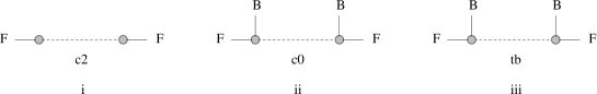
Figure 8: Two point amplitude upto quadratic order in $B$. (i) is due to $\tilde{C}_{2}$ exchange (ii) due to $\tilde{C}_{0}$ exchange and (iii) due to $\tilde{b}$ exchange.

7.2.2 R-R exchange

As in Section 7.2.1, we now expand the Chern-Simons action in terms of the twisted and the untwisted R-R fields. Keeping in mind the background two-form field (7.17) and the relations (7.10). We start with the action for a $D_{5}$ brane wrapping a two cycle ${\cal C}_{1}$.

$$S_{CS} = i\mu_{5}\int_{6}\sum_{n}C_{n}\wedge e^{{\cal B}}$$ (7.30)

$$= i\mu_{3}\frac{1}{2}\left[(2\pi\alpha^{{}^{\prime}})^{2}\int_{4}C_{0}B\wedge b+(2\pi\alpha^{{}^{\prime}})\int_{4}C_{2}\wedge b\right]$$

$$+ i\mu_{3}\frac{1}{4\pi^{2}\alpha^{{}^{\prime}}}\left[(2\pi\alpha^{{}^{\prime}})^{2}\int_{4}\tilde{C}_{0}B\wedge b+(2\pi\alpha^{{}^{\prime}})\int_{4}\tilde{C}_{2}\wedge b\right]$$

Where in the second line of (7.30) we have identified $\mu_{3}=\mu_{5}(4\pi^{2}\alpha^{{}^{\prime}})$. Note that the twisted and untwisted R-R couplings are same as those computed in Section 7.1.2 except for the change in the overall normalisations. The R-R exchanges for the twisted states thus have the same tensor structures as those in Section 7.1.2. Incorporating these changes the two point function with twisted R-R exchanges can easily be computed.

The twisted closed string exchanges in the various limits of $g$ are shown in Figures 8, 9 and 10. We have seen that the untwisted exchanges for both the NS-NS and R-R sectors are the same as those computed in section (7.1) modulo an overall normalisation. The sum of these thus vanishes just like the flat case. This is also what we get from the one loop computation. See eqn(6). The twisted states from both the NS-NS and R-R sectors however sum up to finite results. We write these contributions below with the identification $\kappa_{10}\mu_{3}=\kappa\tau_{3}$.

Figure 9: Two point amplitude upto ${\cal O}(\epsilon^{2})$. (i) is due to $\tilde{C}_{2}$ exchange (ii) due to $\tilde{C}_{0}$ exchange and (iii) due to $\tilde{b}$ exchange.

For small $B$,

$$L_{2} = \frac{i}{{4\pi^{2}}}\kappa_{10}^{2}\mu_{3}^{2}\int\frac{d^{2}k_{\perp}}{(2\pi)^{2}}\frac{1}{k_{\perp}^{2}+p^{2}}\times$$ (7.31)

$$\times [\frac{1}{2}\left[1-(2\pi\alpha^{{}^{\prime}})^{2}\frac{1}{2}\mbox{Tr}(B^{2})\right]\left(\eta^{kk^{{}^{\prime}}}\eta^{ll^{{}^{\prime}}}-\eta^{kl^{{}^{\prime}}}\eta^{lk^{{}^{\prime}}}\right)$$

$$+ (2\pi\alpha^{{}^{\prime}})^{2}\left[\eta^{kk^{{}^{\prime}}}(B^{2})^{ll^{{}^{\prime}}}-\eta^{kl^{{}^{\prime}}}(B^{2})^{lk^{{}^{\prime}}}\right]+(kl)\leftrightarrow(k^{{}^{\prime}}l^{{}^{\prime}})]$$

For $g=\epsilon\eta$,

$$L_{2} = \frac{i}{{4\pi^{2}}}\mbox{det}(2\pi\alpha^{{}^{\prime}}B)\kappa_{10}^{2}\mu_{3}^{2}\int\frac{d^{2}k_{\perp}}{(2\pi)^{2}}\frac{1}{k_{\perp}^{2}+\epsilon^{-1}p^{2}}\times$$ (7.32)

$$\times \frac{\epsilon^{2}}{(2\pi\alpha^{{}^{\prime}})^{4}}\frac{1}{2}\left[\left(\frac{1}{B^{2}}\right)^{kk^{{}^{\prime}}}\left(\frac{1}{B^{2}}\right)^{ll^{{}^{\prime}}}-\left(\frac{1}{B^{2}}\right)^{k^{{}^{\prime}}l}\left(\frac{1}{B^{2}}\right)^{kl^{{}^{\prime}}}\right]$$

$$+ (kl)\leftrightarrow(k^{{}^{\prime}}l^{{}^{\prime}})$$

For $G=\eta$,

$$L_{2} = \frac{i}{{4\pi^{2}}}\mbox{det}(2\pi\alpha^{{}^{\prime}}B)\kappa_{10}^{2}\mu_{3}^{2}\int\frac{d^{2}k_{\perp}}{(2\pi)^{2}}\frac{1}{k_{\perp}^{2}+\tilde{p}^{2}/(2\pi\alpha^{{}^{\prime}})^{2}}\times$$ (7.33)

$$\times \frac{1}{2}\left[\eta^{ll^{{}^{\prime}}}\eta^{kk^{{}^{\prime}}}-\eta^{kl^{{}^{\prime}}}\eta^{lk^{{}^{\prime}}}\right]$$

$$+ (kl)\leftrightarrow(k^{{}^{\prime}}l^{{}^{\prime}})$$

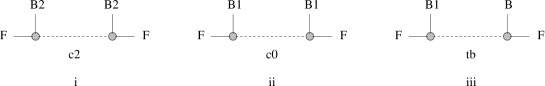
Figure 10: Two point amplitude upto ${\cal O}(\alpha^{{}^{\prime}2})$. (i) is due to $\tilde{C}_{2}$ exchange (ii) due to $\tilde{C}_{0}$ exchange and (iii) due to $\tilde{b}$ exchange.

These expressions are the expansions of the one loop sting amplitude, eqn(6) when $G$ and $\det(g+2\pi\alpha^{{}^{\prime}}B)$ are expanded to respective orders as in equations (4.34), (4.42) and (4.52). We have noted earlier in the bosonic case that the computation of the two point amplitude in string theory sums up all the $B$-field dependence in the open string metric $G$ and $\det(g+2\pi\alpha^{{}^{\prime}}B)$. The analysis in this section again reproduces these terms to the orders relevant in the expansion about the various limits of the closed string metric $g$.

8 Discussions

We now discuss some of the important issues addressed in this article. The central theme has been the world sheet open-closed duality in the presence of $B$-field. The primary motivation for studying this is to see the UV/IR correspondence in noncommutative gauge theories and to identify the exact role played by the $B$-field. World-sheet duality underlies the duality between gravity and gauge theory. An example of which is the AdS/CFT conjecture [1, 2]. On the gauge theory side we have a ${\cal N}=4$ superconformal theory. This theory is finite and hence the duality of the annulus diagram between the open and the closed string channels reduces to a trivial identity namely, $0=0$. For some nontrivial correspondence one must reduce the amount of supersymmetry and break conformal invariance without however bringing in tachyons. In this case one loop amplitudes are divergent. One can compare divergences in the closed and open string channels and if one makes a suitable identification of the cutoffs one can show the equality of amplitudes. We have seen that the $B$-field plays the role of a regulator for the nonplanar diagrams and preserves the duality.

On the gauge theory side, the presence of the $B$-field leads to mixing of UV and IR. The annulus diagram in the Seiberg-Witten limit gives the one loop diagram in noncommutative gauge theory. One also needs to keep only the massless modes propagating in the loop that survive in the $t\rightarrow\infty$ limit. It is important to note that UV divergence in the gauge theory originates from the same region of the modulus as the massless closed string exchanges i.e. $t\rightarrow 0$ end. In general the open string loop UV region is reproduced by closed string trees with small (i.e IR) momentum exchange. A flow-chart of the analysis followed in this article is shown in Figure 11.

Figure 11: Noncommutative field theory and closed string channel limits

$\bullet$ Bosonic Theory

In this bosonic theory, we have seen that the divergences arising from the two ends are related to each other (upto some overall normalisation). This relation could not be made exact in the bosonic setup due to the presence of tachyons, which act as additional sources for divergences. We have shown that the tensor structure for the noncommutative field theory (2.13) two point amplitude can be recovered by considering massless and tachyonic exchanges of closed strings in the presence of background constant $B$-field. For the coefficients to match with the gauge theory result, in the bosonic string case, the full tower of the closed string states are required. We will comment on the closed string couplings below.

$\bullet$ Superstrings on $C^{2}/Z_{2}$

With the lessons from the bosonic theory, in Sections 5 and 6 we have studied a noncommutative ${\cal N}=2$ gauge theory realised on a fractional $D_{3}$-brane localised at the fixed point of $C^{2}/Z_{2}$ orbifold. As discussed above, the UV divergences of the gauge theory comes from the $t\rightarrow 0$ end that is dominated by massless closed strings. In general the massless closed string exchanges account for the UV contribution due to all the open string modes and similarly the dual description of the gauge theory would thus require the contributions from all the massive closed string states as well. This is the situation in the bosonic case. But in this supersymmetric case, the contributions from the massive modes cancel and hence the duality is between the finite number of massless states on both the open and the closed string sides. This is reflected in the equality of (6.15) to the gauge theory amplitude, with both ends regulated in the presence of the $B$-field.

$\bullet$ Closed string couplings

Let us now discuss about the closed string couplings to the noncommutative gauge theory on the brane. Consider for the moment, eqn( 3.7) in the bosonic theory. Let us set $\alpha^{\prime}t=T$

$${\cal A}_{op}\sim\int\frac{dT}{T}(T)^{-\frac{p+1}{2}}\left[e^{2\pi{T\over\alpha^{\prime}}}+(D-2)+O(e^{-2\pi{T\over\alpha^{\prime}}})\right]\exp(-C/T)$$ (8.1)

The $O(1)$ term in the expansion corresponds to the massless open string modes in the loop. If we take the $\alpha^{\prime}\rightarrow 0$ limit the contribution of the massive modes drop out. If we ignore the tachyon we get the massless mode contribution. In the supersymmetric case there is no tachyon. However in the present case dropping the tachyon term makes an exact comparison of the massless sectors of the two cases meaningless because the powers of $\alpha^{\prime}$ cannot match. Nevertheless the comparison is instructive.

The UV contribution of (3.7,8.1), as shown in Figure 1, comes from the region $0<t<1/\Lambda^{2}\alpha^{{}^{\prime}}$. The UV divergences coming from this region is regulated by $C$. In the closed string channel we have,

$${\cal A}_{cl} \sim \int ds(\alpha^{{}^{\prime}})^{-\frac{p+1}{2}}s^{-l/2}\left[e^{2\pi s}+(D-2)+O(e^{-2\pi s})\right]\exp(-Cs/\alpha^{{}^{\prime}})$$ (8.2)

$$\sim (\alpha^{{}^{\prime}})^{-\frac{p+1}{2}}(\alpha^{{}^{\prime}})^{\frac{l}{2}-1}\int d^{l}k_{\perp}\frac{1}{k_{\perp}^{2}+C/\alpha^{{}^{\prime}2}}$$

The $\alpha^{\prime}\rightarrow 0$ limit does not pull out the massless sector (even if we ignore the tachyon) and this makes it clear that in general all the massive closed string modes are required to reproduce the massless open string contribution. But let us focus on the massless states of the closed string sector. In the second expression of (8.2), we have kept only the contribution from the massless closed string mode. This expression can be interpreted as the amplitude of emission and absorption of a closed string state from the $D_{p}$-brane with transverse momentum $k_{\perp}$, integrated over $0<k_{\perp}<1/\Lambda\alpha^{{}^{\prime}}$. The domain of the $k_{\perp}$ integral corresponds to the UV region in the open string channel. $l=D-(p+1)$, is the number of transverse directions in which the closed string propagates. For $l\neq 2$ there is an extra factor of $(\alpha^{{}^{\prime}})^{\frac{l}{2}-1}$ in (8.2) over (3.7), that makes the couplings of the individual closed string modes vanish when compared to the open string channel. It is only for the special case $l=2$ that the powers match.

In the supersymmetric case, for the $C^{2}/Z_{2}$ orbifold, we have seen that the closed strings that contribute to the dual description of the nonplanar divergences are from the twisted sectors. They are free to move in $6$ directions transverse to the orbifold. For the $D_{3}$-brane that is localised at the fixed point with world volume directions perpendicular to the orbifold, these closed string twisted states propagate in exactly two directions transverse to the brane. Thus in this case $l=2$ and from the above discussions this makes the power of $\alpha^{{}^{\prime}}$ in the coupling of closed string with the gauge field strength same as that of the open string channel.

In general, the closed string couplings to the gauge field when the closed string modes are restricted to the massless ones do not give the same normalisation as the gauge theory. The massive closed string modes are expected to contribute so that the normalisations at both the ends are equal. This is guaranteed by open-closed string duality. For the $C^{2}/Z_{2}$ orbifold, the massive states cancel. The finite number of closed string modes thus give the same normalisation as the gauge theory two point function. This is the reason why we are able to see the IR behaviour of noncommutative ${\cal N}=2$ theory in terms of only the massless closed string modes in the twisted sectors.

$\bullet$ Other models

We conclude this article with some comments about other models where this UV/IR correspondence may be seen exactly. In the gauge theory we are able to see the mixing of the UV and IR sectors due to the nature of ultraviolet regulation by the $B$-field. However we have seen that apart from the regulatory nature of the $B$-field, its contribution to the partition function factors out in the determinant (A.18). This means that the $B$-field does not disturb the duality between the massless open/closed modes that may be present in the commutative models. UV/IR correspondence between the noncommutative gauge theory and gravity will thus be naturally manifested in these models. We have seen how this works for the $C^{2}/Z_{2}$ orbifold. Another example is the $C^{3}/(Z_{2}\times Z_{2})$ orbifold that gives ${\cal N}=1$ gauge theory on the fractional $D_{3}$ brane. One may ask whether other such models exist. An analysis on this issue have been made in [43]. Finally, in this article we have only addressed the perturbative nature of this UV/IR correspondence. It will be interesting to explore the non-perturbative aspects of this duality possibly along the lines of [51, 52].

Acknowledgements

This article is based on works with B. Sathiapalan. I would like to thank him for various helpful discussions and for carefully reading this manuscript. I would also like to thank the members of the String Theory groups at University of Roma Tor Vergata and University of Torino for useful discussions.

Appendix A Vacuum amplitude

In this appendix we calculate the vacuum amplitude for the open strings with end points on a $D_{3}$-brane that is located at the fixed point of $C^{2}/Z_{2}$ orbifold. Let us first start with the bosonic part of the world-sheet action,

$$S_{B}=-\frac{1}{4\pi\alpha^{{}^{\prime}}}\int_{\Sigma}g_{MN}\partial_{a}X^{M}\partial^{a}X^{N}+\frac{1}{2}\int_{\partial\Sigma}B_{MN}X^{M}\partial_{\tau}X^{N}$$ (A.1)

The boundary condition for the world-sheet bosons from the above action is,

$$g_{MN}\partial_{\sigma}X^{N}+2\pi\alpha^{{}^{\prime}}B_{MN}\partial_{\tau}X^{N}=0\mid_{\sigma=0,\pi}$$ (A.3)

In the Seiberg-Witten limit, $g_{ij}=\epsilon\eta_{ij}$ we choose the $B$ field along the brane to be of the form,

$$B=\frac{\epsilon}{2\pi\alpha^{{}^{\prime}}}\left(\begin{array}[]{cccc}0&b_{1}&0&0\\ -b_{1}&0&0&0\\ 0&0&0&b_{2}\\ 0&0&-b_{2}&0\end{array}\right)$$ (A.8)

With the above form for the $B$-field, and defining,

$$X_{(1)}^{\pm}=2^{-1/2}(X^{0}\pm X^{1})\mbox{\hskip 14.45377ptand\hskip 14.45377pt}X_{(2)}^{\pm}=2^{-1/2}(X^{2}\pm iX^{3})$$ (A.9)

the boundary condition (A.3) can be rewritten as,

$$\partial_{\sigma}X_{(1)}^{\pm}=\pm b_{1}\partial_{\tau}X_{(1)}^{\pm}\mid_{\sigma=0,\pi}\mbox{\hskip 14.45377ptand\hskip 14.45377pt}\partial_{\sigma}X_{(2)}^{\pm}=\pm ib_{2}\partial_{\tau}X_{(1)}^{\pm}\mid_{\sigma=0,\pi}$$ (A.10)

The mode expansions for the open string satisfying the above boundary conditions are given by,

$$X^{\pm}_{(1)} = x^{\pm}_{(1)}+\frac{2\alpha^{{}^{\prime}}}{1-b_{1}^{2}}(\tau\pm b_{1}\sigma)p^{\pm}_{(1)}+i\sqrt{2\alpha^{{}^{\prime}}}\sum_{n\neq 0}\frac{a^{\pm}_{(1)n}}{n}e^{-i(n\tau\pm\nu_{1})}\cos(n\sigma\mp\nu_{1})$$

$$X^{\pm}_{(2)} = x^{\pm}_{(2)}+\frac{2\alpha^{{}^{\prime}}}{1+b_{2}^{2}}(\tau\pm ib_{2}\sigma)p^{\pm}_{(2)}+i\sqrt{2\alpha^{{}^{\prime}}}\sum_{n\neq 0}\frac{a^{\pm}_{(2)n}}{n}e^{-i(n\tau\pm\nu_{2})}\cos(n\sigma\mp\nu_{2})$$

where we have defined,

$$i\nu_{1}=\frac{1}{2}\log\left(\frac{1+b_{1}}{1-b_{1}}\right)\mbox{\hskip 36.135pt}i\nu_{2}=\frac{1}{2}\log\left(\frac{1+ib_{2}}{1-ib_{2}}\right)$$ (A.12)

The coefficients of the mode expansions (A) are fixed so as to satisfy,

$$\left[X^{+}_{(1)}(\tau,\sigma),P^{-}_{(1)}(\tau,\sigma^{{}^{\prime}})\right]=-2\pi\alpha^{{}^{\prime}}\delta(\sigma-\sigma^{{}^{\prime}})$$ (A.13)

and that the zero modes and the other oscillators satisfy the usual commutation relations,

$$\left[a^{+}_{(1)m},a^{-}_{(1)n}\right]=-m\delta_{m+n}\mbox{\hskip 36.135pt}\left[a^{+}_{(2)m},a^{-}_{(2)n}\right]=m\delta_{m+n}$$ (A.14)

$$\left[x^{+}_{(1)},p^{-}_{(1)}\right]=-i\mbox{\hskip 36.135pt}\left[x^{+}_{(2)},p^{-}_{(2)}\right]=i$$ (A.15)

There is no shift in the moding of the oscillators, the zero point energy and the spectrum is the same as the $B=0$ case. The situation is the same as that of a neutral string in electromagnetic background [45]. Note that the commutator for $X^{\pm}$ now does not vanish at the boundary, for example,

$$\left[X^{+}_{(1)}(\tau,0),X^{-}_{(1)}(\tau,0)\right]=-2\pi i\alpha^{{}^{\prime}}\frac{b_{1}}{1-b_{1}^{2}}$$

$$\left[X^{+}_{(1)}(\tau,\pi),X^{-}_{(1)}(\tau,\pi)\right]=2\pi i\alpha^{{}^{\prime}}\frac{b_{1}}{1-b_{1}^{2}}$$ (A.16)

The zero mode for the energy momentum tensor can now be worked out and is given by,

$$L_{(b)0}^{\parallel}=\frac{2\alpha^{{}^{\prime}}}{b_{1}^{2}-1}p^{+}_{(1)}p^{-}_{(1)}+\frac{2\alpha^{{}^{\prime}}}{b_{2}^{2}+1}p^{+}_{(2)}p^{-}_{(2)}-\sum_{n\neq 0}\left[a^{+}_{(1)-n}a^{-}_{(1)}-a^{+}_{(2)-n}a^{-}_{(2)}\right]$$ (A.17)

Since the spectrum remains the same, the contribution to the vacuum amplitude from the bosonic modes is the same as the usual $B=0$ case except that there is a factor of $\sqrt{(b_{i}^{2}\pm 1)}$ which comes from the trace over the zero modes for each direction along the brane. From (A.8) in the limit (2.5), $b_{i}\sim 1/\sqrt{\epsilon}$ for $B$ to be finite. With this,

$$\epsilon^{2}\prod_{i}^{2}(b_{i}^{2}\pm 1)\rightarrow\det(g+2\pi\alpha^{{}^{\prime}}B)$$ (A.18)

Including contributions from all the directions,

$$L_{(b)0}=L_{(b)0}^{\parallel}+L_{(b)0}^{\perp}+L_{(b)0}^{orb}-\frac{5}{12}$$ (A.19)

$\perp$ denotes the $4,5$ directions and $6,7,8,9$ are the orbifolded directions. Let us now compute the contributions from the world sheet fermions. The action is given by,

$$S_{F}=\frac{i}{4\pi\alpha^{{}^{\prime}}}\int_{\Sigma}g_{MN}\bar{\psi}^{M}\rho^{\alpha}\partial_{\alpha}\psi^{N}-\frac{i}{4}\int_{\partial\Sigma}B_{MN}\bar{\psi}^{N}\rho^{0}\psi^{M}$$ (A.20)

We rewrite the boundary equations from (5.4),

$${}_{MN}(\psi_{L}^{N}-\psi_{R}^{N})+2\pi\alpha^{{}^{\prime}}B_{MN}(\psi_{L}^{N}+\psi_{R}^{N})=0\mid_{\sigma=\pi}$$ (A.21)

$$g_{MN}(\psi_{L}^{M}+(-1)^{a}\psi_{R}^{M})+2\pi\alpha^{{}^{\prime}}B_{MN}(\psi_{L}^{N}-(-1)^{a}\psi_{R}^{N})=0\mid_{\sigma=0}$$ (A.22)

Now defining,

$$\psi_{(1)R,L}^{\pm}=2^{-1/2}(\psi_{R,L}^{0}\pm\psi_{R,L}^{1})\mbox{\hskip 14.45377ptand\hskip 14.45377pt}\psi_{(2)R,L}^{\pm}=2^{-1/2}(\psi_{R,L}^{2}\pm i\psi_{R,L}^{3})$$ (A.23)

For the Ramond Sector $(a=1)$ with the constant $B$-field given by (A.8),

$$\psi_{(1)R}^{\pm}(1\pm b_{1})=\psi_{(1)L}^{\pm}(1\mp b_{1})\mid_{\sigma=0,\pi}$$ (A.24)

Mode expansion,

$$\psi_{(1)L,R}^{\pm}=\sum_{n}d_{(1)n}^{\pm}\chi_{(1)L,R}^{\pm}(\sigma,\tau,n)$$ (A.25)

where,

$$\chi_{(1)R}^{\pm}=\sqrt{2\alpha^{{}^{\prime}}}\exp\{-in(\tau-\sigma)\mp\nu_{1}\}$$ (A.26)

$$\chi_{(1)L}^{\pm}=\sqrt{2\alpha^{{}^{\prime}}}\exp\{-in(\tau+\sigma)\pm\nu_{1}\}$$ (A.27)

and

$$\nu_{1}=\frac{1}{2}\log\left(\frac{1+b_{1}}{1-b_{1}}\right)=\tanh^{-1}b_{1}$$ (A.28)

The boundary condition for the other two directions are,

$$\psi_{(2)R}^{\pm}(1\pm ib_{2})=\psi_{(2)L}^{\pm}(1\mp ib_{2})\mid_{\sigma=0,\pi}$$ (A.29)

This gives the same mode expansion as (A.25),

$$\psi_{(2)L,R}^{\pm}=\sum_{n}d_{(2)n}^{\pm}\chi_{(1)L,R}^{\pm}(\sigma,\tau,n)$$ (A.30)

$$\chi_{(2)R}^{\pm}=\sqrt{2\alpha^{{}^{\prime}}}\exp\{-in(\tau-\sigma)\mp\nu_{2}\}$$ (A.31)

$$\chi_{(2)L}^{\pm}=\sqrt{2\alpha^{{}^{\prime}}}\exp\{-in(\tau+\sigma)\pm\nu_{2}\}$$ (A.32)

and

$$\nu_{2}=\frac{1}{2}\log\left(\frac{1+ib_{2}}{1-ib_{2}}\right)=\tan^{-1}b_{2}$$ (A.33)

Like the bosonic partners there is no shift in the frequencies. The oscillators are integer moded as usual. For the Neveu-Schwarz sector, $(a=0)$, the relative sign between $\psi_{R}^{\pm}$ and $\psi_{L}^{\pm}$ at the $\sigma=\pi$ end in eqn(6) can be brought about by the usual restriction on $n$ to only run over half integers in the mode expansions (A.25,A.30). The oscillators satisfy the standard anticommutation relations,

$$\{d_{(1)n}^{+},d_{(1)m}^{-}\}=-\delta_{m+n}\mbox{\hskip 14.45377pt;\hskip 14.45377pt}\{d_{(2)n}^{+},d_{(2)m}^{-}\}=\delta_{m+n}$$ (A.34)

The zero mode for the energy momentum tensor for the fermions along the brane can be written as,

$$L_{(f)0}^{\parallel}=\sum_{n}n\left[d_{(2)-n}^{-}d_{(2)n}^{+}-d_{(1)-n}^{-}d_{(1)n}^{+}\right]$$ (A.35)

For all the fermions including the contributions from the other directions we have,

$$L_{(f)0}=L_{(f)0}^{\parallel}+L_{(f)0}^{\perp}+L_{(f)0}^{orb}+c_{f}(a)$$ (A.36)

where $L_{(f)0}^{\perp}$ and $L_{(f)0}^{orb}$ have the usual representation in terms of oscillators.

$$c_{f}(1)=\frac{5}{12}\mbox{\hskip 14.45377pt;\hskip 14.45377pt}c_{f}(0)=-\frac{5}{24}$$ (A.37)

We now compute the vacuum amplitude including the contributions from the ghosts. This is given by,

$$Z_{C}={\cal V}_{4}\det(g+2\pi\alpha^{{}^{\prime}}B)\int_{0}^{\infty}\frac{dt}{t}(8\pi^{2}\alpha^{{}^{\prime}}t)^{-2}\mbox{Tr}_{NS-R}\left[\left(\frac{1+g}{2}\right)\left(\frac{1+(-1)^{F}}{2}\right)q^{L_{0}}\right]$$

The origin of the $\det(g+2\pi\alpha^{{}^{\prime}}B)$ term is given in (A.18) and ${\cal V}_{4}$ is the volume of the $D_{3}$-brane and $q=e^{-2\pi t}$. The trace is summed over the spin structures with the orbifold projection. The required traces are listed below in terms of the Theta Functions, $\vartheta_{i}(\nu,it)$.

$$Z\left[\begin{smallmatrix}0\\ 0\end{smallmatrix}\right]_{e}(it) = \mbox{Tr}_{NS}\left[q^{L_{0}}\right]$$ (A.39)

$$= \left[q^{-1/3}\prod_{m=1}^{\infty}(1-q^{m})^{-8}\right]\left[q^{-1/6}\prod_{m=1}^{\infty}(1+q^{m-1/2})^{-8}\right]$$

$$= \eta(it)^{-12}\vartheta^{4}_{3}(0,it)$$

$$Z\left[\begin{smallmatrix}0\\ 1/2\end{smallmatrix}\right]_{e}(it) = \mbox{Tr}_{NS}\left[(-1)^{F}q^{L_{0}}\right]$$ (A.40)

$$= -\left[q^{-1/3}\prod_{m=1}^{\infty}(1-q^{m})^{-8}\right]\left[q^{-1/6}\prod_{m=1}^{\infty}(1-q^{m-1/2})^{-8}\right]$$

$$= -\eta(it)^{-12}\vartheta^{4}_{4}(0,it)$$

$$Z\left[\begin{smallmatrix}1/2\\ 0\end{smallmatrix}\right]_{e}(it) = \mbox{Tr}_{R}\left[q^{L_{0}}\right]$$ (A.41)

$$= -\left[q^{-1/3}\prod_{m=1}^{\infty}(1-q^{m})^{-8}\right]\left[q^{1/3}\prod_{m=1}^{\infty}(1+q^{m})^{8}\right]$$

$$= -\eta(it)^{-12}\vartheta^{4}_{2}(0,it)$$

$$Z\left[\begin{smallmatrix}1/2\\ 1/2\end{smallmatrix}\right]_{e}(it) = \mbox{Tr}_{R}\left[(-1)^{F}q^{L_{0}}\right]=0$$ (A.42)

$$Z\left[\begin{smallmatrix}0\\ 0\end{smallmatrix}\right]_{g}(it)=\mbox{Tr}_{NS}\left[gq^{L_{0}}\right]$$ (A.43)

$$=\left[q^{-1/3}\prod_{m=1}^{\infty}(1-q^{m})^{-4(1+q^{m})^{-4}}\right]\left[q^{1/3}\prod_{m=1}^{\infty}(1+q^{m-1/2})^{4}(1-q^{m-1/2})^{4}\right]$$

$$=4\eta(it)^{-6}\vartheta^{2}_{3}(0,it)\vartheta^{2}_{4}(0,it)\vartheta^{-2}_{2}(0,it)$$

$$Z\left[\begin{smallmatrix}0\\ 1/2\end{smallmatrix}\right]_{g}(it)=\mbox{Tr}_{NS}\left[g(-1)^{F}q^{L_{0}}\right]$$ (A.44)

$$=-\left[q^{-1/3}\prod_{m=1}^{\infty}(1-q^{m})^{-4(1+q^{m})^{-4}}\right]\left[q^{1/3}\prod_{m=1}^{\infty}(1-q^{m-1/2})^{4}(1+q^{m-1/2})^{4}\right]$$

$$=-4\eta(it)^{-6}\vartheta^{2}_{3}(0,it)\vartheta^{2}_{4}(0,it)\vartheta^{-2}_{2}(0,it)$$

$$Z\left[\begin{smallmatrix}1/2\\ 0\end{smallmatrix}\right]_{g}(it) = \mbox{Tr}_{R}\left[gq^{L_{0}}\right]=0$$ (A.45)

$$Z\left[\begin{smallmatrix}1/2\\ 1/2\end{smallmatrix}\right]_{g}(it) = \mbox{Tr}_{R}\left[g(-1)^{F}q^{L_{0}}\right]=0$$

Recalling,

$$\vartheta^{4}_{3}(0,it)-\vartheta^{4}_{4}(0,it)-\vartheta^{4}_{2}(0,it)=0$$ (A.47)

and noting that,

$$Z\left[\begin{smallmatrix}0\\ 0\end{smallmatrix}\right]_{g}(it)=-Z\left[\begin{smallmatrix}0\\ 1/2\end{smallmatrix}\right]_{g}(it)$$ (A.48)

the vacuum amplitude vanishes. This is as a result of supersymmetry.

Theta Functions :

$$q=\exp(-2\pi t)\mbox{\hskip 36.135pt}z=\exp(2\pi i\nu)$$ (A.49)

$$\vartheta_{00}(\nu,it)=\vartheta_{3}(\nu,it)=\prod_{m=1}^{\infty}(1-q^{m})(1+zq^{m-1/2})(1+z^{-1}q^{m-1/2})$$ (A.50)

$$\vartheta_{01}(\nu,it)=\vartheta_{4}(\nu,it)=\prod_{m=1}^{\infty}(1-q^{m})(1-zq^{m-1/2})(1-z^{-1}q^{m-1/2})$$ (A.51)

$$\vartheta_{10}(\nu,it) = \vartheta_{2}(\nu,it)=2\exp(-\pi t/4)\cos(\pi\nu)\times$$ (A.52)

$$\times \prod_{m=1}^{\infty}(1-q^{m})(1+zq^{m-1/2})(1+z^{-1}q^{m-1/2})$$

$$\vartheta_{11}(\nu,it) = \vartheta_{1}(\nu,it)=-2\exp(-\pi t/4)\sin(\pi\nu)\times$$ (A.53)

$$\times \prod_{m=1}^{\infty}(1-q^{m})(1-zq^{m-1/2})(1-z^{-1}q^{m-1/2})$$

$$\eta(it)=q^{1/24}\prod_{m=1}^{\infty}(1-q^{m})$$ (A.54)

Appendix B Eguchi-Hanson Space

In this appendix we give some of the properties of the Eguchi-Hanson space [49] that are used in the analysis in Section 7.2. This space is an euclidean solution of vacuum Einstein equation and is asymptotically locally euclidean. The metric is given by,

$$ds^{2}=f(r)^{-1}dr^{2}+r^{2}f(r)\sigma_{z}^{2}+r^{2}\left[\sigma_{x}^{2}+\sigma_{y}^{2}\right]$$ (B.1)

where,

$$f(r)=\left[1-\left(\frac{a}{r}\right)^{4}\right]\mbox{\hskip 7.22743ptand\hskip 7.22743pt}\sigma_{x}=-\frac{1}{2}\left(\cos{\psi}d\theta+\sin{\theta}\sin{\psi}d\phi\right)$$

$$\sigma_{y}=\frac{1}{2}\left(\sin{\psi}d\theta-\sin{\theta}\cos{\psi}d\phi\right)\mbox{\hskip 7.22743pt}\sigma_{z}=-\frac{1}{2}\left(d\psi+\cos{\theta}d\phi\right)$$

There is an apparent singularity at $r=a$ which is removed if one identifies the range of $\psi$ to be $0\leq\psi\leq 2\pi$. $\theta$ and $\phi$ have the ranges, $0\leq\theta\leq\pi$ and $0\leq\phi\leq 2\pi$. The space near $r=a$ is locally $R^{2}\times S^{2}$. This is seen from the change variables to $u^{2}=r^{2}\left[1-\left(\frac{a}{r}\right)^{4}\right]$, so that for $r=a$ or $u=0$

$$ds^{2}\sim\frac{1}{4}du^{2}+\frac{1}{4}u^{2}\left(d\psi+\cos{\theta}d\phi\right)^{2}+\frac{a^{2}}{4}\left(d\theta^{2}+\sin^{2}{\theta}d\phi^{2}\right)$$ (B.3)

Note that the $R^{2}$ shrinks to a point as $u\rightarrow 0$. As $r\rightarrow\infty$ the constant $r$ hypersurfaces are given by $S^{3}/Z_{2}$. This is due to the fact that the periodicity of $\psi$ here is $2\pi$ instead of the usual periodicity $4\pi$ that gives $S^{3}$. There exists a two-form that is given by,

$$\omega_{2} = \frac{a^{2}}{2\pi}d\left(\frac{\sigma_{z}}{r^{2}}\right)$$ (B.4)

$$= \frac{a^{2}}{2\pi r^{3}}dr\wedge d\psi+\frac{a^{2}}{2\pi r^{3}}\cos{\theta}dr\wedge d\phi+\frac{a^{2}}{4\pi r^{2}}\sin{\theta}d\theta\wedge d\phi$$

It can be checked that this two form satisfies (7.10).

References

- [1] J. M. Maldacena, “The large N limit of superconformal field theories and supergravity,” Adv. Theor. Math. Phys. 2 (1998) 231 [Int. J. Theor. Phys. 38 (1999) 1113] [arXiv:hep-th/9711200]. S. S. Gubser, I. R. Klebanov and A. M. Polyakov, “Gauge theory correlators from non-critical string theory,” Phys. Lett. B 428 (1998) 105 [arXiv:hep-th/9802109]. E. Witten, “Anti-de Sitter space and holography,” Adv. Theor. Math. Phys. 2 (1998) 253 [arXiv:hep-th/9802150].
- [2] A. Hashimoto and N. Itzhaki, “Non-commutative Yang-Mills and the AdS/CFT correspondence,” Phys. Lett. B 465 (1999) 142 [arXiv:hep-th/9907166]. J. M. Maldacena and J. G. Russo, “Large N limit of non-commutative gauge theories,” JHEP 9909 (1999) 025 [arXiv:hep-th/9908134].
- [3] M. R. Douglas and C. M. Hull, “D-branes and the noncommutative torus,” JHEP 9802 (1998) 008 [arXiv:hep-th/9711165].
- [4] V. Schomerus, “D-branes and deformation quantization,” JHEP 9906 (1999) 030 [arXiv:hep-th/9903205].
- [5] F. Ardalan, H. Arfaei and M. M. Sheikh-Jabbari, “Mixed branes and M(atrix) theory on noncommutative torus,” arXiv:hep-th/9803067. F. Ardalan, H. Arfaei and M. M. Sheikh-Jabbari, “Dirac quantization of open strings and noncommutativity in branes,” Nucl. Phys. B 576 (2000) 578 [arXiv:hep-th/9906161].
- [6] C. S. Chu and P. M. Ho, “Noncommutative open string and D-brane,” Nucl. Phys. B 550 (1999) 151 [arXiv:hep-th/9812219].
- [7] N. Seiberg and E. Witten, “String theory and noncommutative geometry,” JHEP 9909 (1999) 032 [arXiv:hep-th/9908142].
- [8] H. S. Snyder, “Quantized Space-Time,” Phys. Rev. 71 (1947) 38. “The Electromagnetic Field in Quantized Space-Time” H. S. Snyder Phys. Rev. 72 (1947) 68.
- [9] A. P. Balachandran, G. Bimonte, E. Ercolessi, G. Landi, F. Lizzi, G. Sparano and P. Teotonio-Sobrinho, “Finite quantum physics and noncommutative geometry,” Nucl. Phys. Proc. Suppl. 37C (1995) 20 [arXiv:hep-th/9403067].
- [10] M. R. Douglas and N. A. Nekrasov, “Noncommutative field theory,” Rev. Mod. Phys. 73 (2001) 977 [arXiv:hep-th/0106048] R. J. Szabo, “Quantum field theory on noncommutative spaces,” Phys. Rept. 378 (2003) 207 [arXiv:hep-th/0109162]. I. Y. Arefeva, D. M. Belov, A. A. Giryavets, A. S. Koshelev and P. B. Medvedev, “Noncommutative field theories and (super)string field theories,” [arXiv:hep-th/0111208].
- [11] S. Minwalla, M. Van Raamsdonk and N. Seiberg, “Noncommutative perturbative dynamics,” JHEP 0002 (2000) 020 [arXiv:hep-th/9912072].
- [12] M. Van Raamsdonk and N. Seiberg, “Comments on noncommutative perturbative dynamics,” JHEP 0003 (2000) 035 [arXiv:hep-th/0002186].
- [13] S. Sarkar and B. Sathiapalan, “Comments on the renormalizability of the broken symmetry phase in noncommutative scalar field theory,” JHEP 0105 (2001) 049 [arXiv:hep-th/0104106]. S. Sarkar, “On the UV renormalizability of noncommutative field theories,” JHEP 0206 (2002) 003 [arXiv:hep-th/0202171].
- [14] F. Ardalan, H. Arfaei and N. Sadooghi, “On the anomalies and Schwinger terms in noncommutative gauge theories,” arXiv:hep-th/0507230.
- [15] S. Vaidya, “UV/IR divergence: to be or not to be,” Talk delivered at, Non Commutative Geometry Workshop, IMSc, Chennai. A. P. Balachandran, G. Mangano, A. Pinzul and S. Vaidya, “Spin and Statistics on the Groenwald-Moyal Plane: Pauli-Forbidden Levels and Transitions,” [arXiv:hep-th/0508002].
- [16] A. P. Balachandran, A. Pinzul and B. A. Qureshi, “UV-IR mixing in non-commutative plane,” arXiv:hep-th/0508151.
- [17] B. Chakraborty, S. Gangopadhyay, A. G. Hazra and F. G. Scholtz, “Twisted Galilean symmetry and the Pauli principle at low energies,” J. Phys. A 39 (2006) 9557 [arXiv:hep-th/0601121].
- [18] H. Grosse and R. Wulkenhaar, “Renormalisation of phi**4 theory on noncommutative R**4 in the matrix base,” Commun. Math. Phys. 256 (2005) 305 [arXiv:hep-th/0401128]. H. Grosse and H. Steinacker, “Renormalization of the noncommutative phi**3 model through the Kontsevich model,” Nucl. Phys. B 746 (2006) 202 [arXiv:hep-th/0512203]. H. Grosse and H. Steinacker, “A nontrivial solvable noncommutative phi**3 model in 4 dimensions,” arXiv:hep-th/0603052.
- [19] C. P. Martin and D. Sanchez-Ruiz, “The one-loop UV divergent structure of U(1) Yang-Mills theory on noncommutative R**4,” Phys. Rev. Lett. 83 (1999) 476 [arXiv:hep-th/9903077]. M. Hayakawa, “Perturbative analysis on infrared aspects of noncommutative QED on R**4,” Phys. Lett. B 478 (2000) 394 [arXiv:hep-th/9912094]. A. Armoni, “Comments on perturbative dynamics of non-commutative Yang-Mills theory,” Nucl. Phys. B 593 (2001) 229 [arXiv:hep-th/0005208].
- [20] N. Ishibashi, S. Iso, H. Kawai and Y. Kitazawa, “Wilson loops in noncommutative Yang-Mills,” Nucl. Phys. B 573 (2000) 573 [arXiv:hep-th/9910004].
- [21] D. J. Gross, A. Hashimoto and N. Itzhaki, “Observables of non-commutative gauge theories,” Adv. Theor. Math. Phys. 4 (2000) 893 [arXiv:hep-th/0008075]. A. Dhar and Y. Kitazawa, “High energy behavior of Wilson lines,” JHEP 0102 (2001) 004 [arXiv:hep-th/0012170]. A. Dhar and Y. Kitazawa, “Wilson loops in strongly coupled noncommutative gauge theories,” Phys. Rev. D 63 (2001) 125005 [arXiv:hep-th/0010256]. S. R. Das and S. J. Rey, “Open Wilson lines in noncommutative gauge theory and tomography of holographic dual supergravity,” Nucl. Phys. B 590 (2000) 453 [arXiv:hep-th/0008042]. S. R. Das and S. P. Trivedi, “Supergravity couplings to noncommutative branes, open Wilson lines and generalized star products,” JHEP 0102 (2001) 046 [arXiv:hep-th/0011131]. M. Rozali and M. Van Raamsdonk, “Gauge invariant correlators in non-commutative gauge theory,” Nucl. Phys. B 608 (2001) 103 [arXiv:hep-th/0012065].
- [22] A. Matusis, L. Susskind and N. Toumbas, “The IR/UV connection in the non-commutative gauge theories,” JHEP 0012 (2000) 002 [arXiv:hep-th/0002075]. F. R. Ruiz, “Gauge-fixing independence of IR divergences in non-commutative U(1), perturbative tachyonic instabilities and supersymmetry,” Phys. Lett. B 502 (2001) 274 [arXiv:hep-th/0012171].
- [23] V. V. Khoze and G. Travaglini, “Wilsonian effective actions and the IR/UV mixing in noncommutative gauge theories,” JHEP 0101 (2001) 026 [arXiv:hep-th/0011218].
- [24] O. Andreev and H. Dorn, “Diagrams of noncommutative Phi**3 theory from string theory,” Nucl. Phys. B 583 (2000) 145 [arXiv:hep-th/0003113].
- [25] Y. Kiem and S. M. Lee, “UV/IR mixing in noncommutative field theory via open string loops,” Nucl. Phys. B 586 (2000) 303 [arXiv:hep-th/0003145].
- [26] A. Bilal, C. S. Chu and R. Russo, “String theory and noncommutative field theories at one loop,” Nucl. Phys. B 582 (2000) 65 [arXiv:hep-th/0003180].
- [27] J. Gomis, M. Kleban, T. Mehen, M. Rangamani and S. H. Shenker, “Noncommutative gauge dynamics from the string worldsheet,” JHEP 0008 (2000) 011 [arXiv:hep-th/0003215].
- [28] H. Liu and J. Michelson, “Stretched strings in noncommutative field theory,” Phys. Rev. D 62 (2000) 066003 [arXiv:hep-th/0004013]. H. Liu and J. Michelson, “*-Trek: The one-loop N = 4 noncommutative SYM action,” Nucl. Phys. B 614 (2001) 279 [arXiv:hep-th/0008205].
- [29] A. Rajaraman and M. Rozali, “Noncommutative gauge theory, divergences and closed strings,” JHEP 0004 (2000) 033 [arXiv:hep-th/0003227].
- [30] S. Chaudhuri and E. G. Novak, “Effective string tension and renormalizability: String theory in a noncommutative space,” JHEP 0008 (2000) 027 [arXiv:hep-th/0006014].
- [31] A. Armoni and E. Lopez, “UV/IR mixing via closed strings and tachyonic instabilities,” Nucl. Phys. B 632 (2002) 240 [arXiv:hep-th/0110113]. A. Armoni, E. Lopez and A. M. Uranga, “Closed strings tachyons and non-commutative instabilities,” JHEP 0302 (2003) 020 [arXiv:hep-th/0301099]. E. Lopez, “From UV/IR mixing to closed strings,” JHEP 0309 (2003) 033 [arXiv:hep-th/0307196].
- [32] S. Sarkar and B. Sathiapalan, “Aspects of open-closed duality in a background B-field,” JHEP 0505 (2005) 062 [arXiv:hep-th/0503009].
- [33] S. Sarkar and B. Sathiapalan, “Aspects of open-closed duality in a background B-field. II,” JHEP 0511 (2005) 002 [arXiv:hep-th/0508004].
- [34] S. Sarkar, “Closed string exchanges on in a background B-field,” JHEP 0605 (2006) 020 [arXiv:hep-th/0602147].
- [35] M. R. Douglas and M. Li, “D-Brane Realization of N=2 Super Yang-Mills Theory in Four Dimensions,” arXiv:hep-th/9604041. M. R. Douglas, D. Kabat, P. Pouliot and S. H. Shenker, “D-branes and short distances in string theory,” Nucl. Phys. B 485 (1997) 85 [arXiv:hep-th/9608024].
- [36] I. R. Klebanov and N. A. Nekrasov, “Gravity duals of fractional branes and logarithmic RG flow,” Nucl. Phys. B 574 (2000) 263 [arXiv:hep-th/9911096].
- [37] M. Bertolini, P. Di Vecchia, M. Frau, A. Lerda, R. Marotta and I. Pesando, “Fractional D-branes and their gauge duals” JHEP 0102 (2001) 014 [arXiv:hep-th/0011077]
- [38] J. Polchinski, “N = 2 gauge-gravity duals,” Int. J. Mod. Phys. A 16, 707 (2001) [arXiv:hep-th/0011193].
- [39] M. Bertolini, P. Di Vecchia, M. Frau, A. Lerda and R. Marotta, “N=2 gauge theories on systems of fractional D3/D7 branes” Nucl. Phys. B 621 (2002) 157 [arXiv:hep-th/0107057]
- [40] M. Bertolini, P. Di Vecchia and R. Marotta, “N = 2 four-dimensional gauge theories from fractional branes,” [arXiv:hep-th/0112195].
- [41] M. Bertolini, “Four lectures on the gauge-gravity correspondence,” Int. J. Mod. Phys. A 18 (2003) 5647 [arXiv:hep-th/0303160]. E. Imeroni, “The gauge / string correspondence towards realistic gauge theories,” [arXiv:hep-th/0312070].
- [42] P. Di Vecchia, A. Liccardo, R. Marotta and F. Pezzella, “Gauge / gravity correspondence from open / closed string duality,” JHEP 0306 (2003) 007 [arXiv:hep-th/0305061]. P. Di Vecchia, A. Liccardo, R. Marotta and F. Pezzella, “Brane-inspired orientifold field theories,” JHEP 0409 (2004) 050 [arXiv:hep-th/0407038].
- [43] P. Di Vecchia, A. Liccardo, R. Marotta and F. Pezzella, “On the gauge / gravity correspondence and the open/closed string duality,” Int. J. Mod. Phys. A 20 (2005) 4699 [arXiv:hep-th/0503156].
- [44] M. A. Namazie, K. S. Narain and M. H. Sarmadi, “Fermionic String Loop Amplitudes With External Bosons,” Phys. Lett. B 177 (1986) 329.
- [45] A. Abouelsaood, C. G. . Callan, C. R. Nappi and S. A. Yost, “Open Strings In Background Gauge Fields,” Nucl. Phys. B 280 (1987) 599. C. G. . Callan, C. Lovelace, C. R. Nappi and S. A. Yost, “String Loop Corrections To Beta Functions,” Nucl. Phys. B 288 (1987) 525.
- [46] J. Polchinski, “String theory. Vol. 1: An introduction to the bosonic string,” Cambridge University Press, Cambridge, (1998)
- [47] S. Mukhi and N. V. Suryanarayana, “Chern-Simons terms on noncommutative branes,” JHEP 0011 (2000) 006 [arXiv:hep-th/0009101]. S. Mukhi and N. V. Suryanarayana, “Gauge-invariant couplings of noncommutative branes to Ramond-Ramond backgrounds,” JHEP 0105 (2001) 023 [arXiv:hep-th/0104045].
- [48] H. Liu and J. Michelson, “Ramond-Ramond couplings of noncommutative D-branes,” Phys. Lett. B 518 (2001) 143 [arXiv:hep-th/0104139]. H. Liu and J. Michelson, “*-trek III: The search for Ramond-Ramond couplings,” Nucl. Phys. B 614 (2001) 330 [arXiv:hep-th/0107172].
- [49] T. Eguchi and A. J. Hanson, “Selfdual Solutions To Euclidean Gravity,” Annals Phys. 120 (1979) 82. T. Eguchi, P. B. Gilkey and A. J. Hanson, “Gravitation, Gauge Theories And Differential Geometry,” Phys. Rept. 66 (1980) 213.
- [50] R. G. Cai and N. Ohta, “On the thermodynamics of large N non-commutative super Yang-Mills theory,” Phys. Rev. D 61 (2000) 124012 [arXiv:hep-th/9910092]. R. G. Cai and N. Ohta, “Noncommutative and ordinary super Yang-Mills on (D(p-2),Dp) bound states,” JHEP 0003 (2000) 009 [arXiv:hep-th/0001213]. R. G. Cai and N. Ohta, “(F1, D1, D3) bound state, its scaling limits and SL(2,Z) duality,” Prog. Theor. Phys. 104 (2000) 1073 [arXiv:hep-th/0007106].
- [51] S. R. Das, S. Kalyana Rama and S. P. Trivedi, “Supergravity with self-dual B fields and instantons in noncommutative gauge theory,” JHEP 0003 (2000) 004 [arXiv:hep-th/9911137
- [52] M. Billo, M. Frau, S. Sciuto, G. Vallone and A. Lerda, “Non-commutative (D)-instantons,” arXiv:hep-th/0511036.