UPR-1155-T, hep-th/0606001
Proton decay via dimension-six operators in
intersecting D6-brane models

Abstract

We analyze the proton decay via dimension six operators in supersymmetric $SU(5)$-Grand Unified models based on intersecting D6-brane constructions in Type IIA string theory orientifolds. We include in addition to $\mathbf{10^{{}^{*}}}\mathbf{10}\mathbf{10}^{{}^{*}}\mathbf{10}$ interactions also the operators arising from $\mathbf{\bar{5}^{{}^{*}}}\mathbf{\bar{5}}\mathbf{10}^{{}^{*}}\mathbf{10}$ interactions. We provide a detailed construction of vertex operators for any massless string excitation arising for arbitrary intersecting D-brane configurations in Type IIA toroidal orientifolds. In particular, we provide explicit string vertex operators for the $\mathbf{10}$ and $\mathbf{\bar{5}}$ chiral superfields and calculate explicitly the string theory correlation functions for above operators. In the analysis we chose the most symmetric configurations in order to maximize proton decay rates for the above dimension six operators and we obtain a small enhancement relative to the field theory result. After relating the string proton decay rate to field theory computations the string contribution to the proton lifetime is $\tau^{ST}_{p}=(0.5-2.1)\times 10^{36}years$, which could be up to a factor of three shorter than that predicted in field theory.

I Introduction

Grand unified theories (GUT’s) Georgi:1974sy not only give a neat and aesthetic description of our four dimensional world but also lead to an explanation of electric charge quantization and - with the aid of supersymmetry - predict the value of $\sin^{2}\theta_{W}$ in very good agreement with the experimental one. Moreover GUT’s lead to Baryon number violating processes; in particular they predict proton decay Langacker:1980js (for a recent review on proton decay see Nath:2006ut ).
In supersymmetric GUT field theories Sakai:1981gr ; Dimopoulos:1981zb the proton decay can occur either by an exchange of a super heavy SUSY particle which corresponds to a decay via the dimension $5$ operator $\int d^{2}\theta\,Q^{3}\,L$ or by a super heavy gauge boson exchange. The latter corresponds to a decay via the dimension $6$ operator $\int d^{4}\theta\,Q^{2}\,\tilde{Q}^{*}\,\tilde{L}^{*}$. In the simplest supersymmetric GUT models, proton decay mediated via dimension $5$ operators dominates and recent computations predict a lifetime for the proton, which is below the present experimental bounds Murayama:2001ur ; Dermisek:2000hr ; Hisano:2000dg , but Emmanuel-Costa:2003pu ; Bajc:2002pg . The fact that proton decay has not yet been observed, suggests the existence of some mechanism that suppresses or even forbids these dimension $5$ operators Bajc:2002bv ; Bajc:2002pg , so that after all the proton decay via dimension six operators FileviezPerez:2004hn is the most dominant one.
In this paper we investigate proton decay via dimension six operators in supersymmetric GUT models based on intersecting D6-brane constructions on type IIA string theory orientifolds. More precisely, we compute the string effects on the proton’s decay into a pion and a positron ($p\rightarrow\pi^{0}e^{+}$) for supersymmetric $SU(5)$-GUT-like models arising from intersecting D6-brane constructions. In $SU(5)$-GUT’s there are two different amplitudes that contribute to this proton decay rate: $\langle\mathbf{10^{{}^{*}}}\mathbf{10}\mathbf{10}^{{}^{*}}\mathbf{10}\rangle$ and $\langle\mathbf{\bar{5}^{{}^{*}}}\mathbf{\bar{5}}\mathbf{10}^{{}^{*}}\mathbf{10}\rangle$, where $\mathbf{\bar{5}}$ and $\mathbf{10}$ denote the multiplets of the gauge group $SU(5)$. For intersecting D6-brane constructions with supersymmetric $SU(5)$-GUT’s Cvetic:2001nr ; Cvetic:2001tj ; Cvetic:2002pj , the latter amplitude was computed in Klebanov:2003my , by explicitly calculating the string amplitude contribution to $\mathbf{10^{{}^{*}}}\mathbf{10}\mathbf{10}^{{}^{*}}\mathbf{10}$ operators. However, even after pushing all the parameters to the limit, in order to maximize the proton decay rate, the string contribution to it is at most comparable to the field theory one. In this work, we explicitly evaluate the amplitude $\langle\mathbf{\bar{5}^{{}^{*}}}\mathbf{\bar{5}}\mathbf{10}^{{}^{*}}\mathbf{10}\rangle$ in the same class of models.
As in Klebanov:2003my , instead of performing the calculation in a specific model, we rather use generic universal features of intersecting D-brane model constructions which are relevant for determining the proton decay rate. In general, the amplitude is sensitive to the local structure of the intersection and the way the D6-branes are wrapped around the compact space. Assuming that the size of the compactified volume is bigger than the string size, the latter effects can be neglected and the computation can be performed for a local D6-brane configuration where we do not need to worry about the embedding in the compact space. This approach allows us to make predictions about the proton decay rate in a general class of intersecting D6-brane orientifold models. In generic models the matter fields $\mathbf{10}$ and $\mathbf{\bar{5}}$ are not located at the same intersection, which leads to an overall suppression of the amplitude $\langle\mathbf{\bar{5}^{{}^{*}}}\mathbf{\bar{5}}\mathbf{10}^{{}^{*}}\mathbf{10}\rangle$. In this work, in order to maximize the effect, we assume the most symmetric case that all the matter arises at intersections that are on top of each other. Therefore, we rather compute an upper bound for the string contribution to the proton decay rate in these models than determining the complete amplitude which is model dependent.
This paper is organized as follows. In section 2 we describe the local setup in which we work and derive the conditions on the intersecting angles, in order to obtain the matter fields in the representation $\mathbf{10}$ and $\mathbf{\bar{5}}$ at the intersection, simultaneously. In section 3 we apply the prescription, given in appendix A, to construct the vertex operators for the matter fields. Section 4 is dedicated to the computation of the string scattering amplitudes, including their normalization. Section 5 states the results of the numerical analysis, while the details can be found in appendix B. In section 6 we relate the string theory results to the four-dimensional field theory and determine the implication of the string scattering amplitude to the proton lifetime. Finally in section 7 we present our conclusions. In appendix A we give a detailed description, how to construct properly vertex operators for strings stretched between two intersecting D-branes.

II Setup

We want to analyze proton decay which occurs due to dimension $6$ operators in a local intersecting D6-brane configuration. Therefore, we have to consider scattering amplitudes of the form $\langle\mathbf{\bar{5}^{{}^{*}}}\mathbf{\bar{5}}\mathbf{10}^{{}^{*}}\mathbf{10}\rangle$ and $\langle\mathbf{10^{{}^{*}}}\mathbf{10}\mathbf{10}^{{}^{*}}\mathbf{10}\rangle$, where $\mathbf{\bar{5}}$ and $\mathbf{10}$ denote the multiplets of the gauge group $SU(5)$. While the latter amplitude was already examined in Klebanov:2003my , we will determine the additional contribution to the proton decay arising from the amplitude $\langle\mathbf{\bar{5}^{{}^{*}}}\mathbf{\bar{5}}\mathbf{10}^{{}^{*}}\mathbf{10}\rangle$.
Since we shall only consider scattering arising at the local intersection, the first step is to derive conditions on the angles so that we have at the local intersection matter fields in the $\mathbf{\bar{5}}$ and $\mathbf{10}$ representation, simultaneously. We will show that this condition is satisfied only for particular regions. For the explicit analysis we shall employ the toroidal orientifold construction and take the size of the tori larger than the inverse string tension, thus suppressing effects due to the world-sheet instantons. In this limit we shall calculate the four-point string amplitudes for the chiral superfields at the D6-brane intersections at the origin of the toroidal orientifold. In that sense the analysis can be applied as the leading order calculation of string amplitudes for the states at the same D6-brane intersection within any orientifold construction.
Let us briefly review the main properties of intersecting D6-models. Generically, one has a number of stacks of D6-branes ($N_{i}$ denotes the number of D-branes for the $i$-th stack), which fill the four-dimensional Minkowski space and intersect each other in the internal space. Open string excitations located at the intersections correspond to four-dimensional chiral fermions transforming in the bifundamental representation $(N_{i},\bar{N}_{j})$, while open strings starting and ending at the same stack of D6-branes transform as seven-dimensional $U(N_{i})$ gauge bosons. In order to make contact with the real world, one has to compactify the six-dimensional internal space which leads to additional consistency conditions on the model called the RR tadpole conditions. D-branes act as sources for the Ramond-Ramond (RR)-charges which need to be canceled due to Gauss’ law in the internal compact space Blumenhagen:2000wh ; Gimon:1996rq . Typically one introduces Orientifold six (O6-) planes, not only because they carry negative RR-charge, but also because they can maintain supersymmetry in the four-dimensional world, while the introduction of anti-D-branes would break all the supersymmetry. The orientifold action leads to image $\text{D6}^{\prime}$-branes and open strings stretched between a D6-brane and its image transform as symmetric or anti-symmetric representation of $U(N_{i})$. As mentioned in the introduction, we rather investigate the proton decay amplitude in a local D6-brane configuration than in a specific model. In the following we discuss all the necessary ingredients for this configuration to obtain a supersymmetric $SU(5)$-GUT like model Cvetic:2002pj (for the non-supersymmetric case see Blumenhagen:2001te ; Axenides:2003hs ).
As explained above the analysis of the D-brane configuration we compactify the internal dimensions are on a factorizable six-torus $T^{6}$. Later we assume that the compactification volume is larger than the string scale so that local effects dominate the amplitude and global ones can be neglected. This assumption also allows us to embed the local D-brane configuration, described below, into an arbitrary compactification manifold.
The complex coordinates of the factorizable six-torus $T^{6}=T^{2}\times T^{2}\times T^{2}$ are given by

$$z_{1}=x^{4}+\mathrm{i}x^{5}\qquad z_{2}=x^{6}+\mathrm{i}x^{7}\qquad z_{1}=x^{8}+\mathrm{i}x^{9}.$$

In order to construct an $SU(5)$ GUT model we shall consider very symmetric configurations of D6-branes. We take a stack $b$ of $M$ D6-branes oriented in the 0123468 directions that coincides with a stack $a$ of $5$ D6 branes along the 0123 directions and forms (supersymmetric) intersecting angles with stack $b$ in the internal toroidal directions. The dimensions 0123 have an interpretation as a $3+1$ dimensional intersecting brane world. Both types of D-branes are wrapped on the $(n^{I},m^{I})$ cycle of the $I^{th}$ torus. Obviously, the wrapping numbers of the stack $b$ are given by

$$b:\,\,\,(n^{1}_{b},m^{1}_{b})(n^{2}_{b},m^{2}_{b})(n^{3}_{b},m^{3}_{b})=(1,0)(1,0)(1,0),$$ (1)

while the one from stack $a$ can take the general form

$$a:\,\,\,(n^{1}_{a},m^{1}_{a})(n^{2}_{a},m^{2}_{a})(n^{3}_{a},m^{3}_{a}).$$ (2)

Given the wrapping numbers, one can compute the intersection angles which are in general given by ($R^{I}_{1}$,$R^{I}_{2}$ denote the radii of the $I^{th}$ torus)

$$\theta^{I}_{ab}=\theta^{I}_{a}-\theta^{I}_{b}=\arctan{\left(\frac{m^{I}_{a}R^{I}_{2}}{n^{I}_{a}R^{I}_{1}}\right)}-\arctan{\left(\frac{m^{I}_{b}R^{I}_{2}}{n^{I}_{b}R^{I}_{1}}\right)}$$

and in our case take the simple form (since $\theta_{b}=0$)

$$\theta^{I}_{ab}=\arctan{\left(\frac{m^{I}_{a}R^{I}_{2}}{n^{I}_{a}R^{I}_{1}}\right)}.$$ (3)

In order to cancel the RR-tadpoles, we must introduce O6-planes and in particular the orientifold action $\Omega R$, where $\Omega$ is the world-sheet parity and $R$ acts by

$$R:(z_{1},z_{2},z_{3})\rightarrow(\bar{z}_{1},\bar{z}_{2},\bar{z}_{3}).$$

This orientifold action forces us to include stacks of image D-branes. Since we chose stack $b$ to lie on top of the orientifold $O6$-plane, it is invariant under the orientifold action: for $M$ coincident branes on top of the $O6$-plane the $\Omega R$ projection leads to the gauge group $Sp(2M)$. For the stack $a$ we have to introduce an image stack $a^{\prime}$ of $5$ D6-branes whose wrapping numbers are given by

$$a^{\prime}:\,\,\,(n^{1}_{a},-m^{1}_{a})(n^{2}_{a},-m^{2}_{a})(n^{3}_{a},-m^{3}_{a})\,\,.$$ (4)

Fermions that arise from strings stretched between $a$ and $a^{\prime}$ transform in the antisymmetric representation of $SU(5)\times SU(5)$, due to the fact that the D-branes intersect at the origin of the torus. Depending on the sign of the intersection number these fermions transform as $\mathbf{10}$’s or $\mathbf{\overline{10}}$’s . Fermions in the $ab$ and $ab^{\prime}$ sector transform in the bifundamental representation $(\mathbf{5},\mathbf{M})$ or $(\mathbf{\bar{5}},\mathbf{M})$ again depending on the sign of the intersection number. In general, the intersection number for two intersecting D-branes $a$ and $b$ is given by

$$I_{ab}=\prod^{3}_{I=1}\,\left(n^{I}_{a}m^{I}_{b}-m^{I}_{a}n^{I}_{b}\right)\,\,.$$ (5)

Now we have all the ingredients to determine the conditions the intersection angles $\theta_{I}$ have to satisfy in order to observe matter fields transforming as $\mathbf{\bar{5}}$ and $\mathbf{10}$ at the intersection, simultaneously. Using (1), (2), (4) and (5) we obtain for the intersection numbers $I_{ab}$ and $I_{aa^{\prime}}$

$$I_{ab}=(-1)^{3}\,\prod^{3}_{I=1}\,m^{I}_{a}\qquad I_{aa^{\prime}}=(-2)^{3}\,\prod^{3}_{I=1}\,n^{I}_{a}m^{I}_{a}\,\,.$$ (6)

Obviously, the sign of the intersection number depends on the sign of the wrapping numbers. For every angle $\theta_{I}$ (from now on we denote $\theta^{I}_{ab}$ by $\theta_{I}$ where $\theta^{I}_{ab}$ is given by (3)) we have to distinguish between four different cases

$$\bullet\,\,n^{I}_{a},\,m^{I}_{a}>0\,\,\,\textrm{which corresponds to an angle with}\,\,\,0<\theta_{I}<\frac{\pi}{2}$$

$$\bullet\,\,n^{I}_{a}>0,\,\,m^{I}_{a}<0\,\,\,\textrm{which corresponds to an angle with}\,\,\,-\frac{\pi}{2}<\theta_{I}<0\qquad$$

$$\bullet\,\,n^{I}_{a}<0\,\,\,m^{I}_{a}>0\,\,\,\textrm{which corresponds to an angle with}\,\,\,\frac{\pi}{2}<\theta_{I}<\pi$$ (7)

$$\bullet\,\,n^{I}_{a},\,m^{I}_{a}<0\,\,\,\textrm{which corresponds to an angle with\,\,\, $-\frac{\pi}{2}<\theta_{I}<-\pi$}\,\,.$$

Since we want to analyze proton decay in a supersymmetric GUT model the choice of the intersection angles $\theta_{I}$ is not arbitrary; the sum has to satisfy Berkooz:1996km

$$\theta_{1}+\theta_{2}+\theta_{3}=0\qquad\mod 2\pi\,\,.$$ (8)

This requirement restricts the choice of the angles. First we consider the case that the angles add up to $0$ and later on we also analyze the configuration where the sums of the angles are $2\pi$ or $-2\pi$. If the sum is equal to $0$ then one or two of the angles have to be negative. If only one angle is negative, let us assume without loss of generality that $\theta_{3}<0$. Since for all angles $|\theta_{I}|\leq\pi$, we distinguish between four different cases for which we obtain, by applying (6) and (II), the intersection numbers and in particular their signs

• $I_{ab}>0$  and  $I_{aa^{\prime}}>0$  for    $0<\theta_{1}<\frac{\pi}{2}\qquad 0<\theta_{2}<\frac{\pi}{2}\qquad-\frac{\pi}{2}<\theta_{3}<0$

• $I_{ab}>0$  and  $I_{aa^{\prime}}<0$  for    $0<\theta_{1}<\frac{\pi}{2}\qquad 0<\theta_{2}<\frac{\pi}{2}\qquad-\pi<\theta_{3}<-\frac{\pi}{2}$

• $I_{ab}>0$  and  $I_{aa^{\prime}}>0$  for    $\frac{\pi}{2}<\theta_{1}<\pi\qquad 0<\theta_{2}<\frac{\pi}{2}\qquad-\pi<\theta_{3}<-\frac{\pi}{2}$

• $I_{ab}>0$  and  $I_{aa^{\prime}}>0$  for    $0<\theta_{1}<\frac{\pi}{2}\qquad\frac{\pi}{2}<\theta_{2}<\pi\qquad-\pi<\theta_{3}<-\frac{\pi}{2}$  .

For all combinations of $\theta_{I}$’s that fulfill the above stated properties ($\sum\theta_{I}=0$ and one angle is negative) we see that the strings stretched between D-branes $a$ and $b$ transform as $\mathbf{5}$ instead of the desired $\mathbf{\bar{5}}$. Therefore we do not observe a 4-point interaction of the form $\mathbf{\bar{5}}^{*}\mathbf{\bar{5}}\mathbf{10}^{*}\mathbf{10}$ at the intersection.
Analyzing the case of two negative angles (without loss of generality we assume that $\theta_{1}$ and $\theta_{2}$ are negative) we again distinguish between four different cases

• $I_{ab}<0$  and  $I_{aa^{\prime}}<0$  for    $-\frac{\pi}{2}<\theta_{1}<0\qquad-\frac{\pi}{2}<\theta_{2}<0\qquad 0<\theta_{1}<\frac{\pi}{2}$

• $I_{ab}<0$  and  $I_{aa^{\prime}}>0$  for    $-\frac{\pi}{2}<\theta_{1}<0\qquad-\frac{\pi}{2}<\theta_{2}<0\qquad\frac{\pi}{2}<\theta_{3}<\pi$

• $I_{ab}<0$  and  $I_{aa^{\prime}}<0$  for    $-\pi<\theta_{1}<-\frac{\pi}{2}\,\,\,\,\,\,\,-\frac{\pi}{2}<\theta_{2}<0\qquad\frac{\pi}{2}<\theta_{3}<\pi$

• $I_{ab}<0$  and  $I_{aa^{\prime}}<0$  for    $-\frac{\pi}{2}<\theta_{1}<0\qquad-\pi<\theta_{2}<-\frac{\pi}{2}\qquad\frac{\pi}{2}<\theta_{3}<\pi$  .

Only in the region $-\frac{\pi}{2}<\theta_{1,2}<0\,,\frac{\pi}{2}<\theta_{3}<\pi$ we observe matter fields transforming as $\mathbf{\bar{5}}$ and $\mathbf{10}$, where strings stretched between the D-branes $a$ and $b$ transform as $\mathbf{\bar{5}}$ and strings stretched between $a$ and $a^{\prime}$ transform as $\mathbf{10}$.
Let us now turn to the case in which the intersection angles $\theta_{I}$ add up to $2\pi$. Then all the angles are positive and we have to distinguish between three different configurations (without loss of generality let us assume that $\theta_{1}$ is always bigger than $\frac{\pi}{2}$)

• $I_{ab}<0$  and  $I_{aa^{\prime}}<0$  for    $\frac{\pi}{2}<\theta_{1}<\pi\qquad\frac{\pi}{2}<\theta_{2}<\pi\qquad 0<\theta_{3}<\frac{\pi}{2}$

• $I_{ab}<0$  and  $I_{aa^{\prime}}<0$  for    $\frac{\pi}{2}<\theta_{1}<\pi\qquad 0<\theta_{2}<\frac{\pi}{2}\qquad\frac{\pi}{2}<\theta_{3}<\pi$

• $I_{ab}<0$  and  $I_{aa^{\prime}}>0$  for    $\frac{\pi}{2}<\theta_{1}<\pi\qquad\frac{\pi}{2}<\theta_{2}<\pi\qquad\frac{\pi}{2}<\theta_{3}<\pi$  .

Again only in one region, $\frac{\pi}{2}<\theta_{1,2,3}<\pi$, we observe matter fields transforming as $\mathbf{\bar{5}}$ and $\mathbf{10}$, where strings stretched between the D-branes $a$ and $b$ transform as $\mathbf{\bar{5}}$ and strings stretched between $a$ and $a^{\prime}$ transform as $\mathbf{10}$.
Finally, we examine the case in which the angles add up to $-2\pi$. Here all three angles have to be negative and again one has to distinguish between three different cases (without loss of generality we assume that $\theta_{1}$ is smaller than $-\frac{\pi}{2}$)

• $I_{ab}>0$  and  $I_{aa^{\prime}}>0$  for    $-\pi<\theta_{1}<\frac{\pi}{2}\qquad-\pi<\theta_{2}<\frac{\pi}{2}\qquad-\frac{\pi}{2}<\theta_{3}<0$

• $I_{ab}>0$  and   $I_{aa^{\prime}}>0$  for    $-\pi<\theta_{1}<\frac{\pi}{2}\qquad-\frac{\pi}{2}<\theta_{2}<0\qquad-\pi<\theta_{3}<-\frac{\pi}{2}$

• $I_{ab}>0$  and   $I_{aa^{\prime}}<0$  for    $-\pi<\theta_{1}<-\frac{\pi}{2}\,\,\,\,\,\,\,-\pi<\theta_{2}<-\frac{\pi}{2}\qquad-\pi<\theta_{3}<-\frac{\pi}{2}$  .

As in the first case, the analysis shows that strings stretched between D-branes $a$ and $b$ transform as $\mathbf{5}$ under the $U(5)$ gauge group. Therefore, at the intersection we do not have any matter fields transforming as $\mathbf{\bar{5}}$.
Summarizing, we determined that only for the two regions $-\frac{\pi}{2}<\theta_{1,2}<0\,,\frac{\pi}{2}<\theta_{3}<\pi$ and $\frac{\pi}{2}<\theta_{1,2,3}<\pi$ we have matter fields transforming as $\mathbf{\bar{5}}$ and $\mathbf{10}$ at the intersection simultaneously. In addition to the amplitude $\langle\mathbf{10^{{}^{*}}}\mathbf{10}\mathbf{10}^{{}^{*}}\mathbf{10}\rangle$, we have for these two regions only, a non-suppressed contribution from $\langle\mathbf{\bar{5}^{{}^{*}}}\mathbf{\bar{5}}\mathbf{10}^{{}^{*}}\mathbf{10}\rangle$ to the proton decay rate. In order to compute these two amplitudes we need the corresponding vertex operators to the states $\mathbf{\bar{5}}$, and $\mathbf{10}$ in the respective configurations, which we determine in the next section.

III Vertex Operators

For different D-brane configurations we have different vacua and therefore different vertex operators. Knowing the D-brane configuration we can use the prescription given in appendix A to obtain the vertex operator for the massless fermion in the R-sector. In this way we can easily determine the vertex operators for $\mathbf{\bar{5}}$, arising from strings stretched between the stacks $a$ and $b$. The vertex operator for $\mathbf{10}$ requires more effort. The simple approach just to replace the $\theta_{I}$ in the $\mathbf{\bar{5}}$ vertex operator by the double, $2\theta_{I}$ only works for $|\theta_{I}|<\frac{1}{2}$, since in the expansion of the bosonic (90) and fermionic degrees of freedom (91) the shift number $\theta_{I}$ has to be in the interval $[-1,1]$. Therefore if $\theta_{I}>\frac{1}{2}$ we need to find an expression $\nu_{I}$ which lies between $0$ and $1$ and describes the D-brane configuration $aa^{\prime}$.

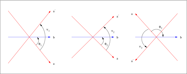
Figure 1: Intersection angles for the case $-\frac{1}{2}<\theta_{1}<0,-\frac{1}{2}<\theta_{2}<0,\frac{1}{2}<\theta_{3}<1$.

Figure 1 which shows the D-brane configuration for the case $-\frac{1}{2}<\theta_{1,2}<0\,,\frac{1}{2}<\theta_{3}<1$. The vertex operator in the $(-\frac{1}{2})$-ghost picture for the massless fermion, arising from a string stretched between D-branes $a$ and $b$ is given by (keep in mind that $\theta_{1,2}$ are negative)

$$V^{-\frac{1}{2}}_{\bar{5}}(z) =\Lambda^{\bar{5}}\,\mathrm{e}^{-\frac{\phi}{2}(z)}\,S^{\alpha}(z)\prod^{2}_{I=1}\sigma_{-\theta_{I}}(z)\,\mathrm{e}^{-\mathrm{i}\left(\theta_{I}+\frac{1}{2}\right)H_{I}(z)}\,\sigma_{1-\theta_{3}}(z)\,\mathrm{e}^{-\mathrm{i}\left(\theta_{3}-\frac{1}{2}\right)H_{3}(z)}\,\mathrm{e}^{\mathrm{i}k\cdot X(z)}.$$ (9)

Now we turn to the $aa^{\prime}$ sector in which the string state transforms as $\mathbf{10}$. We see that the intersection angle in the third complex dimension is given by $\nu_{3}=-2+2\theta_{3}$. Note that the intersection angle $\nu_{3}$ is negative and lies between $-1$ and $0$, since $\theta_{3}$ takes a value between $\frac{1}{2}$ and $1$ and therefore the corresponding vertex operator for the state $\mathbf{10}$ takes the form

$$V^{-\frac{1}{2}}_{10}(z) =\Lambda^{10}\,\mathrm{e}^{-\frac{\phi}{2}(z)}\,S^{\alpha}(z)\prod^{3}_{I=1}\sigma_{1+\nu_{I}}(z)\,\mathrm{e}^{\mathrm{i}\left(\nu_{I}+\frac{1}{2}\right)H_{I}(z)}\,\mathrm{e}^{\mathrm{i}k\cdot X(z)},$$ (10)

where the angles $\nu_{I}$ are given by

$$\nu_{1}=2\theta_{1}\qquad\nu_{2}=2\theta_{2}\qquad\nu_{3}=-2+2\theta_{3}\,\,.$$

Notice, that the angles $\nu_{I}$ add up to $-2$ so that the SUSY condition (8) is satisfied. In an analogous way (look at figure 2), we obtain for the other D-brane configuration

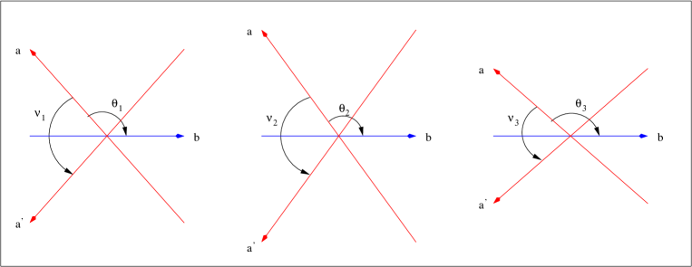
Figure 2: Intersection angles for the case $\frac{1}{2}<\theta_{1}<1,\frac{1}{2}<\theta_{2}<1,\frac{1}{2}<\theta_{3}<1$

• $\frac{1}{2}<\theta_{1}<1\qquad\frac{1}{2}<\theta_{2}<1\qquad\frac{1}{2}<\theta_{3}<1$
  
  For this configuration the vertex operator that creates a string stretched between $a$ and $b$ is

  $$V^{-\frac{1}{2}}_{\bar{5}}(z) =\Lambda^{\bar{5}}\,\mathrm{e}^{-\frac{\phi}{2}(z)}\,S^{\alpha}(z)\prod^{3}_{I=1}\sigma_{1-\theta_{I}}(z)\,\mathrm{e}^{-\mathrm{i}\left(\theta_{I}-\frac{1}{2}\right)H_{I}(z)}\,\mathrm{e}^{\mathrm{i}k\cdot X(z)}\,\,.$$ (11)

  The intersection angles $\nu_{I}$ are given by

  $$\nu_{1}=-2+2\theta_{1}\qquad\nu_{2}=-2+2\theta_{2}\qquad\nu_{3}=-2+2\theta_{3}\,\,.$$

  Obviously, they are all negative, so that the vertex operator which describes the massless $aa^{\prime}$-string in the R-sector takes the form

  $$V^{-\frac{1}{2}}_{10}(z) =\Lambda^{10}\,\mathrm{e}^{-\frac{\phi}{2}(z)}\,S^{\alpha}(z)\prod^{3}_{I=1}\sigma_{1+\nu_{I}}(z)\,\mathrm{e}^{\mathrm{i}\left(\nu_{I}+\frac{1}{2}\right)H_{I}(z)}\,\mathrm{e}^{\mathrm{i}k\cdot X(z)}\,\,.$$ (12)

  Again the angles $\nu_{I}$ add up to $-2$.

In order to calculate scattering amplitudes we also need the vertex operators for $\mathbf{\bar{5}}^{*}$ and $\mathbf{10}^{*}$. We obtain them by replacing the spin field by the spin field with opposite chirality and at the same time sending the angles $\theta_{I}$ and $\nu_{I}$ to $1-\theta_{I}$ and $1-\nu_{I}$, respectively (for negative angle we replace $\theta_{I}$ and $\nu_{I}$ by $-1-\theta_{I}$ and $-1-\nu_{I}$, respectively). For these two cases we obtain

• $-\frac{1}{2}<\theta_{1}<0\qquad-\frac{1}{2}<\theta_{2}<0\qquad\frac{1}{2}<\theta_{3}<1$
  
  

  $$V^{-\frac{1}{2}}_{\bar{5}^{*}}(z) ={\Lambda^{\bar{5}}}^{\dagger}\,\mathrm{e}^{-\frac{\phi}{2}(z)}\,\tilde{S}_{\dot{\alpha}}(z)\prod^{2}_{I=1}\sigma_{1+\theta_{I}}(z)\,\mathrm{e}^{\mathrm{i}\left(\theta_{I}+\frac{1}{2}\right)H_{I}(z)}\,\sigma_{\theta_{3}}(z)\,\mathrm{e}^{\mathrm{i}\left(\theta_{3}-\frac{1}{2}\right)H_{3}(z)}\,\mathrm{e}^{\mathrm{i}k\cdot X(z)}$$ (13)

  for $\mathbf{\bar{5}}^{*}$ and

  $$V^{-\frac{1}{2}}_{10^{*}}(z) ={\Lambda^{10}}^{\dagger}\,\mathrm{e}^{-\frac{\phi}{2}(z)}\,\tilde{S}_{\dot{\alpha}}(z)\prod^{3}_{I=1}\sigma_{-\nu_{I}}(z)\,\mathrm{e}^{-\mathrm{i}\left(\nu_{I}+\frac{1}{2}\right)H_{I}(z)}\,\mathrm{e}^{\mathrm{i}k\cdot X(z)}$$ (14)

  for $\mathbf{10}^{*}$.

• $\frac{1}{2}<\theta_{1}<1\qquad\frac{1}{2}<\theta_{2}<1\qquad\frac{1}{2}<\theta_{3}<1$
  
  

  $$V^{-\frac{1}{2}}_{\bar{5}^{*}}(z) ={\Lambda^{\bar{5}}}^{\dagger}\,\mathrm{e}^{-\frac{\phi}{2}(z)}\,\tilde{S}_{\dot{\alpha}}(z)\prod^{3}_{I=1}\sigma_{\theta_{I}}(z)\,\mathrm{e}^{-\mathrm{i}\left(\theta_{I}-\frac{1}{2}\right)H_{I}(z)}\,\mathrm{e}^{\mathrm{i}k\cdot X(z)}$$ (15)

  for $\mathbf{\bar{5}}^{*}$ and

  $$V^{-\frac{1}{2}}_{{10}^{*}}(z) ={\Lambda^{10}}^{\dagger}\,\mathrm{e}^{-\frac{\phi}{2}(z)}\,\tilde{S}_{\dot{\alpha}}(z)\prod^{3}_{I=1}\sigma_{-\nu_{I}}(z)\,\mathrm{e}^{-\mathrm{i}\left(\nu_{I}+\frac{1}{2}\right)H_{I}(z)}\,\mathrm{e}^{\mathrm{i}k\cdot X(z)}$$ (16)

  for $\mathbf{10}^{*}$ .

Finally, we will discuss the Chan-Paton factors. In a setup without orientifolds strings transform in the bifundamental of $U(N)\times U(M)$. As already mentioned above, the introduction of orientifolds changes the transformation behavior. The full orientifold action on the Chan-Paton factors takes the form

$$\Lambda=-\gamma_{\Omega R}\Lambda^{T}\gamma^{-1}_{\Omega R}\,\,,$$

where $\gamma_{\Omega R}$ is given by Cvetic:2004nk

$$\gamma_{\Omega R}=\left(\begin{array}[]{cccc}0&1_{N}&0&0\\ 1_{N}&0&0&0\\ 0&0&0&1_{M}\\ 0&0&1_{M}&0\\ \end{array}\right)\,\,.$$ (21)

The choice of $N=5$ leads to the following Chan-Paton factors for the $\mathbf{10}$’s

$$\Lambda^{10}=\left(\begin{array}[]{cccc}0&\lambda_{10}&0&0\\ \lambda^{T}_{10}&0&0&0\\ 0&0&0&0\\ 0&0&0&0\\ \end{array}\right)\,\,,$$ (26)

where $\lambda_{10}$ is an antisymmetric $5\times 5$ matrix. For $M$ we choose $1$ that leads to a $Sp(2)$ gauge group on the D-brane $b$ which has two components in the fundamental representation. One component is associated with the matter field $\mathbf{5}$ while the other corresponds to the Higgs particle. Their Chan-Paton factors take the form

$$\Lambda^{\bar{5}}=\left(\begin{array}[]{cccc}0&0&0&0\\ 0&0&\lambda_{\bar{5}}&0\\ 0&0&0&0\\ -\lambda^{T}_{\bar{5}}&0&0&0\\ \end{array}\right)\qquad\qquad\Lambda_{H}=\left(\begin{array}[]{cccc}0&0&0&0\\ 0&0&0&H\\ -H^{T}&0&0&0\\ 0&0&0&0\\ \end{array}\right).$$ (35)

Here $\lambda_{\bar{5}}$ and $H$ are a $5\times 1$ matrices. $\lambda_{10}$ and $\lambda_{\bar{5}}$ denote the usual $10$- and $5$-dimensional representations of the $SU(5)$ gauge group and $H$ is the $5$ dimensional Higgs field in the gauge field theory.

IV String Amplitude

Having derived the vertex operators in the previous section, we have all the ingredients to compute the scattering amplitudes. Assuming that the compactification volume is larger than the string scale worldsheet instantons are suppressed and it is sufficient to compute just the quantum part of the amplitudes. First we will focus on $\langle{V^{\bar{5}}_{-\frac{1}{2}}}^{*}\,V^{\bar{5}}_{-\frac{1}{2}}\,{V^{10}_{-\frac{1}{2}}}^{*}V^{10}_{-\frac{1}{2}}\rangle$ and afterwards we will compute $\langle{V^{10}_{-\frac{1}{2}}}^{*}\,V^{10}_{-\frac{1}{2}}\,{V^{10}_{-\frac{1}{2}}}^{*}V^{10}_{-\frac{1}{2}}\rangle$, which was already examined in Klebanov:2003my

The amplitude $\langle{V^{\bar{5}}_{-\frac{1}{2}}}^{*}\,V^{\bar{5}}_{-\frac{1}{2}}\,{V^{10}_{-\frac{1}{2}}}^{*}V^{10}_{-\frac{1}{2}}\rangle$

We start with the region $-\frac{1}{2}<\theta_{1}<0\,,-\frac{1}{2}<\theta_{2}<0\,,\frac{1}{2}<\theta_{3}<1$ and calculate the amplitude

$$\int\,\prod^{4}_{i=1}\mathrm{d}z_{i}\,\,\langle{V^{\bar{5}}_{-\frac{1}{2}}}^{*}(z_{1})\,V^{\bar{5}}_{-\frac{1}{2}}(z_{2})\,{V^{10}_{-\frac{1}{2}}}^{*}(z_{3})V^{10}_{-\frac{1}{2}}(z_{4})\rangle\,\,,$$

where the vertex operators are in the previous section. Note that all the vertex operators are in the $(-\frac{1}{2})$-ghost pictures, which guarantees a total ghost charge of $-2$ on the disk. Plugging in the vertex operators we see that in order to calculate the amplitude we need the following correlators

$$\begin{gathered}\Big{\langle}\prod_{i=1}^{4}\mathrm{e}^{\mathrm{i}k_{i}\cdot X(z_{i})}\Big{\rangle}=\prod_{\begin{subarray}{c}i,j=1\\ i<j\end{subarray}}^{4}{z_{ij}}^{\alpha^{\prime}\,k_{i}\cdot k_{j}}\qquad\Big{\langle}\mathrm{e}^{-\frac{\phi}{2}(z_{1})}\,\mathrm{e}^{-\frac{\phi}{2}(z_{2})}\,\mathrm{e}^{-\frac{\phi}{2}(z_{3})}\,\mathrm{e}^{-\frac{\phi}{2}(z_{4})}\,\Big{\rangle}=\prod_{\begin{subarray}{c}i,j=1\\ i<j\end{subarray}}^{4}z^{-\frac{1}{4}}_{ij}\\ \\ {\bar{u}^{\dot{\alpha}}}_{1}\,{u_{\alpha}}_{2}\,\bar{u}^{\dot{\beta}}_{3}\,u_{\beta\,4}\,\langle\tilde{S}_{\dot{\alpha}}(z_{1})\,S^{\alpha}(z_{2})\tilde{S}_{\dot{\beta}}(z_{3})S^{\beta}(z_{4})\rangle=\bar{u}_{1}\gamma^{\mu}u_{2}\,\,\bar{u}_{3}\gamma_{\mu}u_{4}\,z^{-\frac{1}{2}}_{13}z^{-\frac{1}{2}}_{24}\,\,,\\ \\ \end{gathered}$$ (41)

where $z_{ij}$ denotes $z_{i}-z_{j}$. The correlator involving the four fermionic twist fields takes an easy form, since we can bosonize the spin fields

$$\Big{\langle}\prod_{i=1}^{4}\mathrm{e}^{\mathrm{i}\,\alpha_{i}H(z_{i})}\Big{\rangle}=\prod_{\begin{subarray}{c}i,j=1\\ i<j\end{subarray}}^{4}{z_{ij}}^{\alpha_{i}\cdot\alpha_{j}}\,\,.$$ (42)

The correlator for the bosonic twist fields is more involved. Using the stress energy tensor method, the quantum part of four bosonic twist fields with two independent angles evaluates to Cvetic:2003ch ; Lust:2004cx

$$\langle\sigma_{1-\theta}(z_{1})\,\sigma_{\theta}(z_{2})\,\sigma_{1-\nu}(z_{3})\,\sigma_{\nu}(z_{4})\rangle=z_{12}^{-\theta(1-\theta)}z_{34}^{-\nu(1-\nu)}\left(\frac{z_{13}\,z_{24}}{z_{14}\,z_{23}}\right)^{\frac{1}{2}(\theta+\nu)-\theta\nu}I^{-\frac{1}{2}}(x)\,\,,$$ (43)

with $x=\frac{z_{12}z_{34}}{z_{13}z_{24}}$ and $I(x)$ is given by

$$I(x)=\frac{1}{2\pi}\big{[}B_{1}(\theta,\nu)\,\overline{G_{2}}(x)H_{1}(1-x)+B_{2}(\theta,\nu)\,G_{1}(x)\overline{H_{2}}(1-x)\big{]}\,\,,$$

where

$$\begin{gathered}B_{1}(\theta,\nu)=\frac{\Gamma(\theta)\,\Gamma(1-\nu)}{\Gamma(1+\theta-\nu)}\qquad B_{2}(\theta,\nu)=\frac{\Gamma(\nu)\,\Gamma(1-\theta)}{\Gamma(1+\nu-\theta)}\\ \\ G_{1}(x)={{}_{2}F}_{1}[\theta,1-\nu,1;x]\qquad G_{2}(x)={{}_{2}F}_{1}[1-\theta,\nu,1;x]\\ \\ H_{1}(x)={{}_{2}F}_{1}[\theta,1-\nu,1+\theta-\nu;x]\qquad H_{2}(x)={{}_{2}F}_{1}[1-\theta,\nu,1-\theta+\nu;x]\,\,.\end{gathered}$$

Applying the correlators, the amplitude becomes

A $$=\mathrm{i}Tr({{\Lambda^{\bar{5}}_{1}}^{\dagger}\,\Lambda_{2}\,{\Lambda^{10}_{3}}^{\dagger}\,\Lambda^{10}_{4}})\,\bar{u}_{1}\gamma^{\mu}u_{2}\,\bar{u}_{3}\gamma_{\mu}u_{4}(2\pi)^{4}\delta^{(4)}\left(\sum^{4}_{i=1}k_{i}\right)$$

$$\qquad\times\int\,\prod^{4}_{i=1}\mathrm{d}z_{i}\frac{\left[I\left(-\theta_{1},1+\nu_{1},x\right)\,I\left(-\theta_{2},1+\nu_{2},x\right)\,I\left(1-\theta_{3},1+\nu_{3},x\right)\right]^{-\frac{1}{2}}}{(z_{12}\,z_{34})^{\alpha^{\prime}\,s+1}\,(z_{13}\,z_{24})^{\alpha^{\prime}\,t}(z_{14}\,z_{23})^{\alpha^{\prime}\,u+1}}\,\,,$$

where $s$, $t$ and $u$ are the Mandelstam variables

$$s=-(k_{1}+k_{2})^{2}\qquad t=-(k_{1}+k_{3})^{2}\qquad u=-(k_{1}+k_{4})^{2}\,.$$

The conformal Killing group can be used to fix three of the vertex operator positions. A convenient choice is

$$z_{1}=0\qquad z_{2}=x\qquad z_{3}=1\qquad z_{4}=z_{\infty}=\infty\,\,,$$

which implies the $c$-ghost contribution

$$\langle\,c\,(0)\,\,c\,(1)\,\,c\,(z_{\infty})\rangle=z^{2}_{\infty}\,\,.$$

After fixing three positions, we are left with an integral over one worldsheet variable

A $$=\mathrm{i}C_{A}\,Tr({{\Lambda^{\bar{5}}_{1}}^{\dagger}\,\Lambda^{\bar{5}}_{2}\,{\Lambda^{10}_{3}}^{\dagger}\,\Lambda^{10}_{4}})\,\bar{u}_{1}\gamma^{\mu}u_{2}\,\bar{u}_{3}\gamma_{\mu}u_{4}(2\pi)^{4}\delta^{(4)}\left(\sum^{4}_{i=1}k_{i}\right)$$

$$\qquad\times\int^{1}_{0}\,\mathrm{d}x\,\frac{\left[I\left(-\theta_{1},1+\nu_{1},x\right)\,I\left(-\theta_{2},1+\nu_{2},x\right)\,I\left(1-\theta_{3},1+\nu_{3},x\right)\right]^{-\frac{1}{2}}}{x^{\alpha^{\prime}\,s+1}(1-x)^{\alpha^{\prime}\,u+1}}.$$

In order to obtain the full amplitude we need to sum over all possible orderings

$$\emph{A}_{total}= \text{C}\,\Big{(}Tr({{\Lambda^{\bar{5}}_{1}}^{\dagger}\,\Lambda^{\bar{5}}_{2}\,\Lambda^{10}_{4}\,{\Lambda^{10}_{3}}^{\dagger}}+Tr({\Lambda^{\bar{5}}_{2}\,{\Lambda^{\bar{5}}_{1}}^{\dagger}\,{\Lambda^{10}_{3}}^{\dagger}}\,\Lambda^{10}_{4})\Big{)}\int^{0}_{-\infty}\mathrm{d}x\,U(x)$$

$$\text{C}\,\Big{(}Tr({{\Lambda^{\bar{5}}_{1}}^{\dagger}\,\Lambda^{\bar{5}}_{2}\,{\Lambda^{10}_{3}}^{\dagger}\,\Lambda^{10}_{4}}+Tr({\Lambda^{\bar{5}}_{2}\,{\Lambda^{\bar{5}}_{1}}^{\dagger}\,\Lambda^{10}_{4}\,{\Lambda^{10}_{3}}^{\dagger}})\Big{)}\int^{1}_{0}\,\,\mathrm{d}x\,U(x)$$

$$\text{C}\,\Big{(}Tr({{\Lambda^{\bar{5}}_{1}}^{\dagger}\,{\Lambda^{10}_{3}}^{\dagger}\,\Lambda^{\bar{5}}_{2}\,\Lambda^{10}_{4}}+Tr({{\Lambda^{\bar{5}}_{1}}^{\dagger}\,\Lambda^{10}_{4}\,\Lambda^{\bar{5}}_{2}\,{\Lambda^{10}_{3}}^{\dagger}})\Big{)}\int^{\infty}_{1}\mathrm{d}x\,U(x)\,\,,$$

with

$$\text{C}=\mathrm{i}\,C_{A}\,\bar{u}_{1}\gamma^{\mu}u_{2}\,\bar{u}_{3}\gamma_{\mu}u_{4}(2\pi)^{4}\delta^{(4)}\left(\sum^{4}_{i=1}k_{i}\right)$$

and

$$U(x) =\frac{\left[I\left(-\theta_{1},1+\nu_{1},x\right)\,I\left(-\theta_{2},1+\nu_{2},x\right)\,I\left(1-\theta_{3},1+\nu_{3},x\right)\right]^{-\frac{1}{2}}}{x^{\alpha^{\prime}\,s+1}(1-x)^{\alpha^{\prime}\,u+1}}\,\,.$$

Calculating the traces for the third term by plugging in the respective Chan-Paton factors immediately shows that they vanish. Explicit computation of the traces leads to the identities $Tr({{\Lambda^{\bar{5}}_{1}}^{\dagger}\,\Lambda^{\bar{5}}_{2}\,{\Lambda^{10}_{3}}^{\dagger}\,\Lambda^{10}_{4}})=Tr({\Lambda^{\bar{5}}_{2}\,{\Lambda^{\bar{5}}_{1}}^{\dagger}\,\Lambda^{10}_{4}\,{\Lambda^{10}_{3}}^{\dagger}})$ and $Tr({{\Lambda^{\bar{5}}_{1}}^{\dagger}\,\Lambda^{\bar{5}}_{2}\,\Lambda^{10}_{4}\,{\Lambda^{10}_{3}}^{\dagger}})=Tr({\Lambda^{\bar{5}}_{2}\,{\Lambda^{\bar{5}}_{1}}^{\dagger}\,{\Lambda^{10}_{3}}^{\dagger}\,\Lambda^{10}_{4}})$ and thus the amplitude takes the form

$$A_{total}=2\mathrm{i}C_{A}\, \bar{u}_{1}\gamma^{\mu}u_{2}\,\bar{u}_{3}\gamma_{\mu}u_{4}(2\pi)^{4}\delta^{(4)}\left(\sum^{4}_{i=1}k_{i}\right)$$

$$\times\Big{(}Tr({{\Lambda^{\bar{5}}_{1}}^{\dagger}\,\Lambda^{\bar{5}}_{2}\,{\Lambda^{10}_{3}}^{\dagger}\,\Lambda^{10}_{4}})K(\theta_{1},\theta_{2},\theta_{3})+Tr({{\Lambda^{\bar{5}}_{1}}^{\dagger}\,\Lambda^{\bar{5}}_{2}\,\Lambda^{10}_{4}\,{\Lambda^{10}_{3}}^{\dagger}})T(\theta_{1},\theta_{2},\theta_{3})\Big{)},$$ (44)

with

$$K(\theta_{1},\theta_{2},\theta_{3})=\int^{1}_{0}\,\,\mathrm{d}x\,U(x)\qquad T(\theta_{1},\theta_{2},\theta_{3})=\int^{0}_{-\infty}\,\,\mathrm{d}x\,U(x).$$ (45)

In the field theory, the first term corresponds to proton decay via a gauge boson, while the second one describes the proton decay mediated via a Higgs particle, arising from the Yukawa interaction $\mathbf{10}\,\mathbf{\bar{5}}\,\mathbf{\bar{5}_{H}}$.
Finally we replace the $\nu$’s by the angles $\theta$

$$\nu_{1}=2\theta_{1}\qquad\nu_{2}=2\theta_{2}\qquad\nu_{3}=-2+2\theta_{3}$$

and obtain for $U$

$$U(x) =\frac{\left[I\left(-\theta_{1},1+2\theta_{1},x\right)I\left(-\theta_{2},1+2\theta_{2},x\right)\,I\left(1-\theta_{3},-1+2\theta_{3},x\right)\right]^{-\frac{1}{2}}}{x^{\alpha^{\prime}\,s+1}(1-x)^{\alpha^{\prime}\,u+1}}\,\,.$$ (46)

Applying the same procedure for the other sector we obtain

• $\frac{1}{2}<\theta_{1}<1\qquad\frac{1}{2}<\theta_{2}<1\qquad\frac{1}{2}<\theta_{3}<1$
  
  The amplitude

  $$\int\,\prod^{4}_{i=1}\mathrm{d}z_{i}\,\,\langle{V^{\bar{5}}_{-\frac{1}{2}}}^{*}(z_{1})\,V^{\bar{5}}_{-\frac{1}{2}}(z_{2})\,{V^{10}_{-\frac{1}{2}}}^{*}(z_{3})V^{10}_{-\frac{1}{2}}(z_{4})\rangle\,\,,$$

  takes the form

  $$\emph{A}_{total}= 2\mathrm{i}C_{A}\,\bar{u}_{1}\gamma^{\mu}u_{2}\,\bar{u}_{3}\gamma_{\mu}u_{4}\,(2\pi)^{4}\delta^{(4)}\left(\sum^{4}_{i=1}k_{i}\right)$$ (47)

  $$\,\,\,\times\Big{(}Tr({{\Lambda^{\bar{5}}_{1}}^{\dagger}\,\Lambda^{\bar{5}}_{2}\,{\Lambda^{10}_{3}}^{\dagger}\,\Lambda^{10}_{4}})K(\theta_{1},\theta_{2},\theta_{3})+Tr({{\Lambda^{\bar{5}}_{1}}^{\dagger}\,\Lambda^{\bar{5}}_{2}\,\Lambda^{10}_{4}\,{\Lambda^{10}_{3}}^{\dagger}})T(\theta_{1},\theta_{2},\theta_{3})\Big{)}\,\,,$$

  with $K$ and $T$ defined in (45) and $U$ given by

  $$U(x) =x^{-\alpha^{\prime}\,s-1}(1-x)^{-\alpha^{\prime}\,u-1}\prod^{3}_{I=1}[I(1-\theta_{I},-1+2\theta_{I},x)]^{-\frac{1}{2}}\,\,.$$ (48)

The amplitude $\langle{V^{10}_{-\frac{1}{2}}}^{*}\,V^{10}_{-\frac{1}{2}}\,{V^{10}_{-\frac{1}{2}}}^{*}V^{10}_{-\frac{1}{2}}\rangle$

Note that in both cases, $\frac{1}{2}<\theta_{1,2}<1\,,-\frac{1}{2}<\theta_{3}<0$ and $\frac{1}{2}<\theta_{1,2,3}<1$, the vertex operators for the matter fields transforming as $\mathbf{10}$ take the same form. Thus the computation of the amplitude $\langle{V^{10}_{-\frac{1}{2}}}^{*}\,V^{10}_{-\frac{1}{2}}\,{V^{10}_{-\frac{1}{2}}}^{*}V^{10}_{-\frac{1}{2}}\rangle$ is identical for both cases. We use the same correlators stated above except for the one involving the bosonic twist fields, which takes a simpler form, since it involves only one independent angle Cvetic:2003ch

$$\langle\sigma_{1-\theta}(z_{1})\,\sigma_{\theta}(z_{2})\,\sigma_{1-\theta}(z_{3})\,\sigma_{\theta}(z_{4})\rangle=\left(\frac{z_{13}\,z_{24}}{z_{12}\,z_{14}\,z_{23}\,z_{34}}\right)^{\theta(1-\theta)}\,L^{-\frac{1}{2}}(x)$$ (49)

with

$$L(x)=\frac{1}{\sin(\pi\,\theta)}\,_{2}F_{1}[\theta,1-\theta,1,x]\,_{2}F_{1}[\theta,1-\theta,1,1-x].$$

Plugging in all the correlators and fixing three vertex operator positions we obtain

$$\emph{A}_{total} =\mathrm{i}\,C_{A}^{\prime}\Big{(}Tr({{\Lambda^{10}_{1}}^{\dagger}\,\Lambda^{10}_{2}\,{\Lambda^{10}_{3}}^{\dagger}\,\Lambda^{10}_{4}})+Tr({{\Lambda^{10}_{1}}^{\dagger}\,\Lambda^{10}_{4}\,{\Lambda^{10}_{3}}^{\dagger}\,\Lambda^{10}_{2}})\Big{)}\,(2\pi)^{4}\delta^{(4)}\left(\sum^{4}_{i=1}k_{i}\right)$$

$$\qquad\qquad\qquad\times\bar{u}_{1}\gamma^{\mu}u_{2}\,\bar{u}_{3}\gamma_{\mu}u_{4}\int^{1}_{0}\mathrm{d}x\,x^{-\alpha^{\prime}\,s-1}\,(1-x)^{-\alpha^{\prime}\,u-1}\prod^{3}_{I=1}L^{-\frac{1}{2}}(1+\nu_{I},x)\,\,.$$

Finally we replace the $\nu_{I}$ by $\theta_{I}$ and obtain

• $-\frac{1}{2}<\theta_{1}<0\qquad-\frac{1}{2}<\theta_{2}<0\qquad\frac{1}{2}<\theta_{3}<1$
  

  $$\emph{A}_{total} =\mathrm{i}C_{A}^{\prime}Tr\Big{(}{\Lambda^{10}_{1}}^{\dagger}\Lambda^{10}_{2}{\Lambda^{10}_{3}}^{\dagger}\Lambda^{10}_{4}+{\Lambda^{10}_{1}}^{\dagger}\Lambda^{10}_{4}{\Lambda^{10}_{3}}^{\dagger}\Lambda^{10}_{2}\Big{)}$$

  $$\qquad\qquad\qquad\times(2\pi)^{4}\delta^{(4)}\left(\sum^{4}_{i=1}k_{i}\right)\bar{u}_{1}\gamma^{\mu}u_{2}\,\bar{u}_{3}\gamma_{\mu}u_{4}\,M(\theta_{1},\theta_{2},\theta_{3})$$ (50)

  with

  $$M(\theta_{1},\theta_{2},\theta_{3})=\int^{1}_{0}\mathrm{d}x\,\frac{x^{-\alpha^{\prime}\,s-1}\,(1-x)^{-\alpha^{\prime}\,u-1}}{L^{\frac{1}{2}}(1+2\theta_{1},x)\,L^{\frac{1}{2}}(1+2\theta_{2},x)\,L^{\frac{1}{2}}(-1+2\theta_{3},x)}\,\,.$$ (51)

• $\frac{1}{2}<\theta_{1}<1\qquad\frac{1}{2}<\theta_{2}<1\qquad\frac{1}{2}<\theta_{3}<1$
  

  $$\emph{A}_{total} =\mathrm{i}C_{A}^{\prime}Tr\Big{(}{\Lambda^{10}_{1}}^{\dagger}\Lambda^{10}_{2}{\Lambda^{10}_{3}}^{\dagger}\Lambda^{10}_{4}+{\Lambda^{10}_{1}}^{\dagger}\Lambda^{10}_{4}{\Lambda^{10}_{3}}^{\dagger}\Lambda^{10}_{2}\Big{)}$$

  $$\qquad\qquad\qquad\times(2\pi)^{4}\delta^{(4)}\left(\sum^{4}_{i=1}k_{i}\right)\bar{u}_{1}\gamma^{\mu}u_{2}\,\bar{u}_{3}\gamma_{\mu}u_{4}\,M(\theta_{1},\theta_{2},\theta_{3})$$ (52)

  with

  $$M(\theta_{1},\theta_{2},\theta_{3})=\int^{1}_{0}\mathrm{d}x\,\frac{x^{-\alpha^{\prime}\,s-1}\,(1-x)^{-\alpha^{\prime}\,u-1}}{L^{\frac{1}{2}}(2\theta_{1}-1,x)\,L^{\frac{1}{2}}(2\theta_{2}-1,x)\,L^{\frac{1}{2}}(2\theta_{3}-1,x)}\,\,.$$ (53)

The $\langle{V^{10}_{-\frac{1}{2}}}^{*}\,V^{10}_{-\frac{1}{2}}\,{V^{10}_{-\frac{1}{2}}}^{*}V^{10}_{-\frac{1}{2}}\rangle$ does not involve an Higgs exchange, since couplings of the form $\mathbf{10}\,\mathbf{10}\,\mathbf{5_{H}}$ are absent due to the $U(1)$ charge conversation Cvetic:2002pj .

Normalization

In this section we determine the two undetermined constants $C_{A}$ and $C^{\prime}_{A}$ in the string amplitudes computed above. We will use the fact that even in the low energy limit the integrals (45), (51) and (53) are convergent in the limit $x\rightarrow 0$, which corresponds to a gauge boson exchange. Factorizing the amplitude into two three point functions allows us to normalize it. We start with the amplitude $\langle{V^{\bar{5}}_{-\frac{1}{2}}}^{*}\,V^{\bar{5}}_{-\frac{1}{2}}\,{V^{10}_{-\frac{1}{2}}}^{*}V^{10}_{-\frac{1}{2}}\rangle$ and turn later to $\langle{V^{10}_{-\frac{1}{2}}}^{*}\,V^{10}_{-\frac{1}{2}}\,{V^{10}_{-\frac{1}{2}}}^{*}V^{10}_{-\frac{1}{2}}\rangle$.

The amplitude $\langle{V^{\bar{5}}_{-\frac{1}{2}}}^{*}\,V^{\bar{5}}_{-\frac{1}{2}}\,{V^{10}_{-\frac{1}{2}}}^{*}V^{10}_{-\frac{1}{2}}\rangle$

We first examine the limit $x\rightarrow 0$ and will see that even in the low energy limit the integral is convergent, due to the special kinematics of this problem.

Limit $x\rightarrow 0$

As $x\rightarrow 0$ the hypergeometric functions behave like

$$F(a,b,1,x)\rightarrow 1\qquad F(a,b,a+b,1-x)\rightarrow\frac{\Gamma(a+b)}{\Gamma(a)\Gamma(b)}\,\,\ln\left(\frac{\kappa(a,b)}{x}\right)\,\,,$$ (54)

with

$$\ln{\kappa(a,b)}=2\psi(1)-\psi(a)-\psi(b)\,\,.$$

Applying (54) $I$ takes the form

$$\lim_{x\rightarrow 0}I(\theta,\nu,x)=\frac{1}{\sqrt{\pi}}\,\ln\left(\frac{\delta(\theta,\nu)}{x}\right)\,\,,$$

where $\ln\delta(\theta,\nu)$ is given by

$$\ln\delta(\theta,\nu)=2\psi(1)-\frac{1}{2}\psi(\theta)-\frac{1}{2}\psi(1-\theta)-\frac{1}{2}\psi(\nu)-\frac{1}{2}\psi(1-\nu)\,\,.$$

Therefore even for $s=t=0$ we obtain for the integral (44) a convergent expression in the limit $x\rightarrow 0$

$$\sim\pi^{3/2}\,\int_{0}\frac{\mathrm{d}x}{x}\,\ln[1/x]^{-3/2}\,\,.$$ (55)

That allows us to normalize the amplitude by factorizing the amplitude in the limit $x\rightarrow 0$, where it reduces to a product of two three-point functions

$$A_{4}(k_{1},k_{2},k_{3},k_{4})=\frac{\mathrm{i}}{2}\int\frac{\mathrm{d}^{7}k\,\mathrm{d}^{7}k^{{}^{\prime}}}{(2\pi)^{7}}\,\,\frac{\sum_{IJ\mu}A^{I\mu}_{j}(k_{1},k_{2},k)A^{I\mu}_{j}(k_{3},k_{4},k^{{}^{\prime}})\delta(k-k^{{}^{\prime}})}{k^{2}-\mathrm{i}\epsilon}\,\,.$$ (56)

The unusual factor of $\frac{1}{2}$ is introduced to take into account the doubling in the Chan-Paton factors.
The three-point amplitudes describe the exchange of a gauge boson and are given by

$$A^{\mu}(k_{1},k_{2},k_{3})=\mathrm{i}\,g_{D_{6}}\,(2\pi)^{4}\delta^{(4)}\left(\sum^{3}_{i=1}k_{i}\right)\bar{u}_{1}\gamma^{\mu}u_{2}Tr({\Lambda^{\bar{5}}_{1}}^{\dagger}\,\Lambda^{\bar{5}}_{2}\,\Lambda_{A})\,\,.$$ (57)

Here $\mu$ corresponds to the polarization and $\Lambda_{A}$ denote the Chan Paton factors of the gauge boson. The latter takes the form

$$\Lambda_{A}=\left(\begin{array}[]{cccc}\lambda_{a}&0&0&0\\ 0&\lambda_{a}&0&0\\ 0&0&0&0\\ 0&0&0&0\\ \end{array}\right)\,,$$ (62)

where the $\lambda_{a}$’s are the gauge bosons of $U(5)$ which satisfy $Tr(\lambda_{a}\,\lambda_{b})=\frac{1}{2}\delta_{ab}$. The intermediate state is a massless $a-a$ string, which is a gauge boson, that can carry arbitrary momentum $p$ along the directions of the D-brane $a$ orthogonal to the intersection. In these directions we have to integrate over

$$\int\mathrm{d}^{3}q\,\int_{0}\mathrm{d}x\,x^{\alpha^{\prime}\,q^{2}-\alpha^{\prime}\,s-1}=\pi^{3/2}\,(\alpha^{\prime})^{-3/2}\,\int_{0}\mathrm{d}x\,x^{-\alpha^{\prime}\,s-1}\,[\ln(1/x)]^{-3/2}$$

which tells us that the replacement, going from effective field theory in four dimensions to the form of the string integrand near $x=0$ is no longer

$$\frac{1}{s}\rightarrow\alpha^{\prime}\,\int_{0}\mathrm{d}x\,x^{-\alpha^{\prime}\,s-1}\,\,,$$

but

$$\int\frac{\mathrm{d}^{3}q}{q^{2}-s}\rightarrow\pi^{3/2}(\alpha^{\prime})^{-1/2}\int_{0}\mathrm{d}x\,x^{-\alpha^{\prime}\,s-1}\,[\ln(1/x)]^{-3/2}\,\,.$$ (63)

Performing the integral on the right hand side of (56) and using the replacement (63) we obtain

$$\mathrm{i}\frac{g^{2}_{D_{6}}\pi^{5/2}}{2\alpha^{\prime 1/2}}\,Tr({{\Lambda^{\bar{5}}_{1}}^{\dagger}\,\Lambda^{\bar{5}}_{2}\,{\Lambda^{10}_{3}}^{\dagger}\,\Lambda^{10}_{4}})\,\bar{u}_{1}\gamma^{\mu}u_{2}\,\bar{u}_{3}\gamma_{\mu}u_{4}\,\delta^{(4)}\left(\sum^{4}_{i=1}k_{i}\right)\int_{0}\,\mathrm{d}x\,x^{-\alpha^{\prime}\,s-1}\,[\ln(1/x)]^{-3/2}.$$ (64)

This needs to be the same as (44) in the limit $x\rightarrow 0$

$$2\mathrm{i}\,C_{A}\,Tr({{\Lambda^{\bar{5}}_{1}}^{\dagger}\,\Lambda^{\bar{5}}_{2}\,{\Lambda^{10}_{3}}^{\dagger}\,\Lambda^{10}_{4}})\,\bar{u}_{1}\gamma^{\mu}u_{2}\,\bar{u}_{3}\gamma_{\mu}u_{4}(2\pi)^{4}\,\pi^{3/2}\delta^{(4)}\left(\sum^{4}_{i=1}k_{i}\right)\int_{0}\,\mathrm{d}x\,x^{-s-1}\,[\ln(1/x)]^{-3/2}\,\,,$$

which leads us with $g^{2}_{D_{6}}=(2\pi)^{4}\alpha^{\prime 3/2}g_{s}$ to the normalization constant $C_{A}$

$$C_{A}=\frac{\pi}{2}\,g_{s}\,\alpha^{\prime}\,\,.$$ (65)

For the second amplitude one obtains, following the same procedure, the same normalization constant.

The amplitude $\langle{V^{10}_{-\frac{1}{2}}}^{*}\,V^{10}_{-\frac{1}{2}}\,{V^{10}_{-\frac{1}{2}}}^{*}V^{10}_{-\frac{1}{2}}\rangle$

Note that the amplitude is invariant under the exchange of $x$ and $1-x$ if one simultaneously interchanges $s$ and $u$. Therefore we obtain similar limits for $x\rightarrow 0$ and $x\rightarrow 1$. That is not too surprising taking into account that we expect an exchange of a gauge boson in both limits.

Limit $x\rightarrow 0$ and $x\rightarrow 1$

Using (54) and taking the low energy limit $s,t\rightarrow 0$ we get for $x\rightarrow 0$

$$\sim\pi^{3/2}\,\int_{0}\frac{\mathrm{d}x}{x}\,\ln[1/x]^{-3/2}$$ (66)

and a similar result for $x\rightarrow 1$

$$\sim\pi^{3/2}\,\int^{1}\frac{\mathrm{d}x}{1-x}\,\ln[1/(1-x)]^{-3/2}\,\,.$$ (67)

Following the same procedure as in the case of the amplitude $\langle{V^{\bar{5}}_{-\frac{1}{2}}}^{*}\,V^{\bar{5}}_{-\frac{1}{2}}\,{V^{10}_{-\frac{1}{2}}}^{*}V^{10}_{-\frac{1}{2}}\rangle$ we obtain for normalization constant ${C_{A}}^{\prime}$

$$C_{A}^{\prime}=\pi g_{s}\,\alpha^{\prime}\,\,.$$ (68)

V Numerical analysis

We want to compute the contribution of the amplitude which arises from the four-Fermi interaction in the low energy effective theory. That means that we take the low energy limit and subtract the $s$, $t$ and $u$ poles, if present. It turns out that the amplitudes are divergent only in the limit $x\rightarrow-\infty$. As derived in appendix B there is no massless exchange in the $u$-channel. The s-channel requires more explanation, since in general we expect a massless gauge boson exchange, which leads to an undesired s-pole. We saw that the integral does not diverge at the s-pole, since we neglected global effects coming from the internal space. Locally, the internal dimensions look like a flat space with infinite volume which leads to a vanishing gauge coupling in four dimensions

$${g_{YM}}^{2}\sim\frac{1}{V_{int}}\,\,,$$ (69)

here $V_{int}$ denotes the internal volume and $g_{YM}$ is the gauge coupling in four dimensions. Thus even if we observe a gauge boson exchange, we do not see an $s$-pole in our effective low energy theory. In the limit $x\rightarrow-\infty$, which corresponds to a $t$-pole, the integral is divergent and in order to obtain the four-Fermi interaction we have to subtract this pole. A detailed discussion of the numerical analysis of the integrals $K$,$T$ and $M$ in the amplitudes (44),(47), (50) and (52) can be found in appendix B, where for simplification we set $\theta_{1}=\theta_{2}=\theta$.

$-\frac{1}{2}<\theta_{1}<0\,\,\,-\frac{1}{2}<\theta_{2}<0\,\,\,\frac{1}{2}<\theta_{3}<1$				$\frac{1}{2}<\theta_{1}<1\,\,\,\,\,\frac{1}{2}<\theta_{2}<1\,\,\,\,\,\frac{1}{2}<\theta_{3}<1$
$\theta$	$K$	$T$	$M$	$\theta$	$K$	$T$	$M$
-.40	6.5	5.4	10.3	.505	1.5	1.5	2.5
-.42	5.7	5.1	9.4	.51	2.0	2.1	3.5
-.44	4.9	4.6	8.3	.52	2.9	2.9	4.9
-.46	4.0	4.0	6.9	.54	4.0	4.0	6.9
-.48	2.9	2.9	4.9	.56	4.9	4.6	8.3
-.49	2.0	2.1	3.5	.58	5.7	5.1	9.4
-.495	1.5	1.5	2.5	.60	6.5	5.4	10.3

Table 1: Contribution to $K$, $T$ and $M$ for different angles $\theta$

Table 1 shows the contribution $M$ for the string amplitude $\langle{V^{10}_{-\frac{1}{2}}}^{*}\,V^{10}_{-\frac{1}{2}}\,{V^{10}_{-\frac{1}{2}}}^{*}V^{10}_{-\frac{1}{2}}\rangle$ and the contributions $K$ and $T$ arise from $\langle{V^{\bar{5}}_{-\frac{1}{2}}}^{*}\,V^{\bar{5}}_{-\frac{1}{2}}\,{V^{10}_{-\frac{1}{2}}}^{*}V^{10}_{-\frac{1}{2}}\rangle$ for different angles $\theta$. For $\theta=-1/3$ and $\theta=2/3$ we observe a second massless fermion which indicates that we now have $N=2$ supersymmetry. Since our world is chiral we choose $\theta$ in the ranges, given in table 1.
Note also, that going from the first sector $-\frac{1}{2}<\theta_{1}<0\,,-\frac{1}{2}<\theta_{2}<0\,,\frac{1}{2}<\theta_{3}<1$ to the second one $\frac{1}{2}<\theta_{1}<1\,,\frac{1}{2}<\theta_{2}<1\,,\frac{1}{2}<\theta_{3}<1$ and replacing $\theta$ by $1-\theta$, simultaneously leads to the same results for $K$, $T$ and $M$. This is not too surprising, since the respective vertex operators correspond to the same states if you interchange $\theta$ with $1-\theta$.

VI Comparison to Four-Dimensional Field theory

In this section we want to compare the amplitude obtained due to massive string states in string theory with the amplitude on the field theory side. Therefore, we would like to replace all the string theory parameters such as the string coupling $g_{s}$ or the gauge coupling $g_{D6}$ by appropriate expressions using quantities about which we have some knowledge of, such as $M_{GUT}$ and $\alpha_{GUT}$. We follow closely the analysis of Klebanov:2003my .
The action for the gauge fields living on the $D6$-branes is

$$\frac{1}{4g^{2}_{D_{6}}}\int\mathrm{d}^{7}x\,\text{Tr}F_{ij}F^{ij}\,\,,$$

where the $F_{ij}$ is the Yang-Mills field strength and Tr denotes the trace in the fundamental representation of $U(N)$. After compactification on $R\times Q$ the action becomes

$$\frac{V_{Q}}{4g^{2}_{D_{6}}}\int\mathrm{d}^{4}x\,\text{Tr}F_{ij}F^{ij},$$

where $V_{Q}$ is the volume of $Q$. Keeping in mind the usual convention $Tr(Q_{a}Q_{b})=\frac{1}{2}\delta_{ab}$ we finally obtain for the action

$$\frac{V_{Q}}{8g^{2}_{D_{6}}}\int\mathrm{d}^{4}x\,\text{Tr}F_{ij}F^{ij}.$$ (70)

On the other hand, the GUT action is given by

$$\frac{1}{4g^{2}_{GUT}}\int\mathrm{d}^{4}x\,\text{Tr}F_{ij}F^{ij}\,\,,$$ (71)

where $g_{GUT}$ is the GUT coupling. Comparing (70) and (71), along with $g^{2}_{D_{6}}=(2\pi)^{4}g_{s}\alpha^{\prime 3/2}$ Polchinski:1998rr and $\alpha_{{}_{GUT}}=g^{2}_{{}_{GUT}}/(4\pi)$, leads to the identification

$$\alpha^{\prime}=\left(\frac{\alpha_{{}_{GUT}}\,V_{Q}}{(2\pi)^{3}\,g_{s}}\right)^{2/3}\,\,.$$ (72)

The volume $V_{Q}$ enters into the running of the $SU(3)\times SU(2)\times U(1)$ gauge coupling from high energies to low energies. Approximately, one can say that $V^{-1/3}_{Q}$ plays the role of the mass scale unification $M_{GUT}$ in four dimensions. In order to obtain the exact relation between them one needs to compute the one loop threshold correction to the gauge coupling, which was done for M-theory on a manifold of $G_{2}$ holonomy Friedmann:2002ty

$$V_{Q}=\frac{L(Q)}{M^{3}_{GUT}}\,\,,$$ (73)

where $L(Q)$ is a topological invariant, the Ray-Singer torsion. In Klebanov:2003my it is argued that this relation holds true in Type IIA string theory and thus we finally obtain

$$\alpha^{\prime}=\left(\frac{\alpha_{{}_{GUT}}\,L(Q)}{(2\pi)^{3}\,g_{s}\,M^{3}_{GUT}}\right)^{2/3}\,\,.$$ (74)

We would like to replace all the string parameters in the amplitudes (44) and (47) in terms of four dimensional field theory quantities. Unfortunately, equation (74) still includes two string parameters $L(Q)$ and $g_{s}$. The Ray-Singer torsion $L(Q)$ depends crucially on the compact space and takes for simple lens spaces values around $8$ Friedmann:2002ty . In order to neglect higher order loop amplitudes the string coupling $g_{s}$ is better smaller than $1$. On the other hand we are interested in the largest possible contribution to the enhancement and set therefore $g_{s}$ approximately to 1.

Field theory amplitude

After relating the string parameters to four dimensional field theory constants, of which we have some experimental knowledge, we now recall the analysis of proton decay in the $SU(5)$ GUT model. This treatment closely follows Langacker:1980js .
The kinetic energy for an $SU(5)$ gauge theory, involving the gauge field $A$, the fermionic field $\psi_{\bar{5}}$, which transforms as $\mathbf{\bar{5}}$, and the fermionic field $\psi_{10}$ transforming as 10 under the $SU(5)$ takes the form

$$T=\frac{1}{4g^{2}_{{}_{GUT}}}Tr(F^{2}(A))+\mathrm{i}\bar{\psi}_{\bar{5}}\gamma^{\mu}D_{\mu}\psi_{\bar{5}}+\mathrm{i}\bar{\psi}_{10}\gamma^{\mu}D^{\prime}_{\mu}\psi_{10}$$ (75)

with

$$D_{\mu}{\psi_{\bar{5}}}^{a}=\partial_{\mu}\,{\psi_{\bar{5}}}^{a}-\frac{\mathrm{i}\,g_{{}_{GUT}}}{\sqrt{2}}\,{(A_{\mu})}^{a}_{b}\,{\psi_{\bar{5}}}^{b}$$

and

$$D^{\prime}_{\mu}{\psi_{10}}^{ab}=\partial_{\mu}\,{\psi_{10}}^{ab}-\frac{\mathrm{i}\,g_{{}_{GUT}}}{\sqrt{2}}\,{(A_{\mu})}^{a}_{c}\,{\psi_{10}}^{cb}-\frac{\mathrm{i}\,g_{{}_{GUT}}}{\sqrt{2}}\,{(A_{\mu})}^{b}_{d}\,{\psi_{10}}^{ad}\,\,.$$

By explicitly using the antisymmetry of $\psi_{10}$, the latter can be simplified to

$$D^{\prime}_{\mu}{\psi_{10}}^{ab}=\partial_{\mu}\,{\psi_{10}}^{ab}-\frac{\mathrm{i}\,2g_{{}_{GUT}}}{\sqrt{2}}\,{(A_{\mu})}^{a}_{c}\,{\psi_{10}}^{cb}.$$

The gauge field $A$ can be displayed as a $5\times 5$ matrix

$$A_{\mu}=\left(\begin{array}[]{cccccc}&&&|&{X^{C}_{1}}_{\mu}&{Y^{C}_{1}}_{\mu}\\ &\frac{1}{\sqrt{2}}\sum_{a}G^{a}_{\mu}\lambda^{a}&&|&{X^{C}_{2}}_{\mu}&{Y^{C}_{2}}_{\mu}\\ &&&|&{X^{C}_{3}}_{\mu}&{Y^{C}_{3}}_{\mu}\\ ---&---&---&+&---&---\\ {X_{1}}_{\mu}&{X_{2}}_{\mu}&{X_{3}}_{\mu}&&\frac{W^{3}_{\mu}}{\sqrt{2}}&W^{+}_{\mu}\\ {Y_{1}}_{\mu}&{Y_{2}}_{\mu}&{Y_{3}}_{\mu}&|&W^{-}_{\mu}&-\frac{W^{3}_{\mu}}{\sqrt{2}}\\ \end{array}\right)+\frac{B_{\mu}}{\sqrt{30}}\left(\begin{array}[]{ccccc}-2&&&&\\ &-2&&&\\ &&-2&&\\ &&&3&\\ &&&&3\end{array}\right)\,\,,$$

where the $\lambda^{a}$ are the Gell-Mann matrices, the $G^{a}_{\mu}$ denote the gluon fields of $SU(3)$ and $W^{+}_{\mu}$, $W^{-}_{\mu}$, $W^{3}_{\mu}$, $B_{\mu}$ are the bosons of the $SU(2)\times U(1)$. The $X$ and $Y$ are the new gauge bosons that are contained in $SU(5)$ and do not occur in the standard model. The exchange of these new gauge bosons leads to Baryon-Lepton number violating processes and therefore allows proton decay.
To make contact to the standard model the $SU(5)$ needs to be broken, which will be achieved by giving the Higgs field, which transforms under the $24$-dimensional adjoint representation of $SU(5)$ an expectation value. This generates a mass $M_{X}$ of order of $10^{16}$ Gev for the gauge bosons $X$ and $Y$.
From (75) one can easily deduce the effective four-Fermi interactions which lead to proton decay. Ignoring mixing effects as well as second and third families one obtains for the

$$L_{eff}=\frac{g^{2}_{{}_{GUT}}}{2\,M^{2}_{X}}\Big{(}\varepsilon_{\alpha\,\beta\,\gamma}\,\bar{u}^{C\gamma}_{L}\,\gamma^{\mu}\,u^{\beta}_{L}\Big{)}\,\Big{(}2\bar{e}^{+}_{L}\,\gamma_{\mu}\,d^{\alpha}_{L}+\bar{e}^{+}_{R}\,\gamma_{\mu}\,d^{\alpha}_{R}\Big{)}\,\,,$$ (76)

where the first factor arises from a $\mathbf{10}^{*}\,\mathbf{10}\,\mathbf{10}^{*}\,\mathbf{10}$ interaction and the second factor from a $\mathbf{\bar{5}}^{*}\,\mathbf{\bar{5}}\,\mathbf{10}^{*}\,\mathbf{10}$ interaction .

Comparison

This result (76) we want to compare with the string theory contribution. In order to do that we turn on Wilson lines, that break the $SU(5)$ gauge group into the standard model ones. Assuming such a mechanism of symmetry breaking exist we compute the traces of (44) and (50) only for entries which lead to proton decay. One obtains for (44) and (47)

$$A^{\bar{5}\bar{5}1010}_{total}=\mathrm{i}\,(2\pi)^{4}\delta^{(4)}\left(\sum^{4}_{i=1}k_{i}\right)\,\pi g_{s}\alpha^{\prime}\Big{(}\varepsilon_{\alpha\,\beta\,\gamma}\,\bar{u}^{C\gamma}_{L}\,\gamma^{\mu}\,u^{\beta}_{L}\Big{)}\,\Big{(}\bar{e}^{+}_{R}\,\gamma_{\mu}\,d^{\alpha}_{R}\Big{)}\left(K(\theta)+T(\theta)\right)$$ (77)

and for (50) and (52)

$$\emph{A}^{10101010}_{total} =2\mathrm{i}\,(2\pi)^{4}\delta^{(4)}\left(\sum^{4}_{i=1}k_{i}\right)\,\pi g_{s}\,\alpha^{\prime}\Big{(}\varepsilon_{\alpha\,\beta\,\gamma}\,\bar{u}^{C\gamma}_{L}\,\gamma^{\mu}\,u^{\beta}_{L}\Big{)}\,\Big{(}\bar{e}^{+}_{L}\,\gamma_{\mu}\,d^{\alpha}_{L}\Big{)}\,M(\theta)\,.$$ (78)

Comparing the string theory proton decay rate with the one from four dimensional gauge theory one obtains

$$\frac{\Gamma_{ST}(p\rightarrow\pi^{0}\,e^{+})}{\Gamma_{FT}(p\rightarrow\pi^{0}\,e^{+})}=\left(\frac{g^{1/3}_{s}\,L(Q)^{2/3}}{8\pi^{2}\alpha^{1/3}_{{}_{GUT}}}\right)^{2}\,\left(\frac{M_{X}}{M_{{}_{GUT}}}\right)^{4}\,\left(\frac{(K+T)^{2}+4M^{2}}{4}\right)\,.$$ (79)

Most recent calculations Hisano:2000dg for the proton decay mediated via gauge bosons in an $SU(5)$-GUT model gave the lifetime $\tau^{FT}_{p}$ in terms of gauge boson mass $M_{X}$ and $\alpha_{{}_{GUT}}$

$$\tau^{FT}_{p}=1.6\times 10^{36}years\left(\frac{0.04}{\alpha_{{}_{GUT}}}\right)^{2}\left(\frac{M_{X}}{20^{16}GeV}\right)^{4}\,\,.$$ (80)

This leads with the values $M_{X}=M_{{}_{GUT}}=2\times 10^{16}GeV$ and $\alpha_{{}_{GUT}}=0.04$ to a proton lifetime of $1.6\times 10^{36}years$. The present lower bound on the proton lifetime for $p\rightarrow\pi^{0}\,e^{+}$ is $1.6\times 10^{33}years$ Eidelman:2004wy and even the next generation proton decay experiments, based on underground water Cherenkov detectors will reach a lower bound not larger than $10^{35}years$ Jung:1999jq . Therefore in the near future, unless there is an enhancement to the proton decay amplitude, we will not observe the proton decay via gauge boson exchange. Using (79) and (80) the proton lifetime in the considered type IIA string models is

$$\tau^{ST}_{p}\approx 1.6\times 10^{36}years\frac{54^{2}}{L^{4/3}(Q)\,g^{2/3}_{s}\,((K+T)^{2}+4M^{2})}\left(\frac{0.04}{\alpha_{GUT}}\right)^{4/3}\left(\frac{M_{{}_{GUT}}}{20^{16}GeV}\right)^{4}\,\,,$$ (81)

where $\frac{L^{4/3}(Q)\,g^{2/3}_{s}\,((K+T)^{2}+4M^{2})}{54^{2}}$ is the string enhancement factor. Note that in (81) the heavy gauge boson mass $M_{X}$, which is model dependent, is absent and the proton lifetime depends only on $M_{{}_{GUT}}$. We also observe an anomalous power of $\alpha_{{}_{GUT}}$ in (81) indicating the stringy nature of the enhancement.
Let us examine the enhancement factor $\frac{L^{4/3}(Q)\,g^{2/3}_{s}\,((K+T)^{2}+4M^{2})}{54^{2}}$. As already mentioned earlier the Ray-Singer torsion is around $8$ for lens spaces with small fundamental group. The string coupling takes values between $0$ and $1$, but in order to obtain the largest possible enhancement to the proton decay amplitude we assume it is approximately $1$. Table 1 shows that $M$ ranges between $5$ and $10$, while $K+T\approx 1.2\times M$, leading with the numerical four-dimensional $SU(5)$ supersymmetric values $M_{{}_{GUT}}=2\times 10^{16}GeV$ and $\alpha_{{}_{GUT}}=0.04$ to a proton lifetime $\tau^{ST}_{p}=(0.5-2.1)\times 10^{36}years$. We see that although there is in addition to the contribution to the four-Fermi interaction which in field theory are due to gauge boson exchange, there is also a contribution due to terms that in field theory arise from Higgs particle exchange, the total string contribution is not large enough to lead to a considerable enhancement in the proton decay rate.
The dimension six operators $\mathbf{\bar{5}^{{}^{*}}}\mathbf{\bar{5}}\mathbf{10}^{{}^{*}}\mathbf{10}$ have in contrast to the operators $\mathbf{10^{{}^{*}}}\mathbf{10}\mathbf{10}^{{}^{*}}\mathbf{10}$ a second proton decay mode; they lead in addition to the decay mode $p\rightarrow\pi^{0}\,e^{+}$ also to $p\rightarrow\pi^{+}\bar{\nu}$. Plugging in the respective entries in (44) leading to the mode $p\rightarrow\pi^{+}\bar{\nu}$ one obtains

$$A^{\bar{5}\bar{5}1010}_{total}=\mathrm{i}\,(2\pi)^{4}\delta^{(4)}\left(\sum^{4}_{i=1}k_{i}\right)\,\pi g_{s}\alpha^{\prime}\Big{(}\varepsilon_{\alpha\,\beta\,\gamma}\,\bar{u}^{C\gamma}_{L}\,\gamma^{\mu}\,d^{\beta}_{L}\Big{)}\,\Big{(}\bar{\nu}^{C}_{R}\,\gamma_{\mu}\,d^{\alpha}_{R}\Big{)}\left(K(\theta)+T(\theta)\right)\,\,.$$ (82)

Within the field theory the effective interaction

$$L_{eff}=\frac{g^{2}_{{}_{GUT}}}{2\,M^{2}_{X}}\Big{(}\varepsilon_{\alpha\,\beta\,\gamma}\,\bar{u}^{C\gamma}_{L}\,\gamma^{\mu}\,d^{\beta}_{L}\Big{)}\,\Big{(}\bar{\nu}^{C}_{R}\,\gamma_{\mu}\,d^{\alpha}_{R}\Big{)}\,\,,$$ (83)

the ratio between the proton decay rates is given by

$$\frac{\Gamma_{ST}(p\rightarrow\pi^{+}\,\bar{\nu})}{\Gamma_{FT}(p\rightarrow\pi^{+}\,\bar{\nu})}=\left(\frac{g^{1/3}_{s}\,L(Q)^{2/3}}{16\pi^{2}\alpha^{1/3}_{{}_{GUT}}}\right)^{2}\,\left(\frac{M_{X}}{M_{{}_{GUT}}}\right)^{4}\,\Big{(}K+T\Big{)}^{2}\,\,.$$ (84)

For this decay mode the string enhancement to the proton decay rate is even smaller than for the mode $p\rightarrow\pi^{0}\,e^{+}$ due to the absence of the $\mathbf{10^{{}^{*}}}\mathbf{10}\mathbf{10}^{{}^{*}}\mathbf{10}$ interaction term. For the same choice of parameter as above (in addition we assume that $M_{X}=M_{GUT}$) the ratio (84) takes values between $0.2$ and $0.8$.

VII Conclusions

In this paper we computed the local, string contribution to the proton decay rate for supersymmetric SU(5) GUT’s based on intersecting D6-brane constructions in Type IIA string theory orientifolds by explicitly calculating the string amplitude contribution to the dimension six operators. If the compactification volume is larger than the string scale, world-sheet instanton effects are negligible and the local contribution is the dominant one. In the computation presented, we assumed that the matter fields $\mathbf{\bar{5}}$ and $\mathbf{10}$ are located at the same intersections on top of each other, and thus the leading string amplitude contributions have no suppressions from area factors. In this case the amplitudes give the largest possible contribution to the proton decay rate. In contrast to the authors Klebanov:2003my , who only considered the amplitude $\langle\mathbf{10^{{}^{*}}}\mathbf{10}\mathbf{10}^{{}^{*}}\mathbf{10}\rangle$, we also included the explicit calculation of the string amplitude for $\mathbf{\bar{5}^{{}^{*}}}\mathbf{\bar{5}}\mathbf{10}^{{}^{*}}\mathbf{10}$ operators.
As a by-product we explicitly constructed the vertex operators for any massless string excitation at supersymmetric D-brane intersections arising in Type IIA toroidal orientifolds. Specifically, by employing explicit string vertex operators for the $\mathbf{10}$ and $\mathbf{\bar{5}}$ chiral superfields, we calculated explicitly string theory amplitudes contributing to the proton decay via dimension six operators. In the analysis we chose the most symmetric configurations in order to maximize proton decay rates for the above dimension six operators and we obtain a small enhancement relative to the field theory result. In contrast to the string amplitude $\langle\mathbf{10^{{}^{*}}}\mathbf{10}\mathbf{10}^{{}^{*}}\mathbf{10}\rangle$, where only the gauge boson exchange contributes to the proton decay rate for the amplitude $\langle\mathbf{\bar{5}^{{}^{*}}}\mathbf{\bar{5}}\mathbf{10}^{{}^{*}}\mathbf{10}\rangle$ there is an additional contribution corresponding to the proton decay mediated via Higgs particle.
After relating the string theory result to the field theory computations we obtain for the proton lifetime in type IIA string theory models

$$\tau^{ST}_{p}\approx 1.6\times 10^{36}years\frac{54^{2}}{L^{4/3}(Q)\,g^{2/3}_{s}\,((K+T)^{2}+4M^{2})}\left(\frac{.04}{\alpha_{GUT}}\right)^{4/3}\left(\frac{M_{{}_{GUT}}}{20^{16}GeV}\right)^{4}\,\,,$$ (85)

which has an anomalous power of $\alpha_{GUT}$ indicating the string effects. The string enhancement factor depends on the Ray-Singer torsion, the string coupling $g_{s}$ and the numerical quantities $M$, $K$ and $T$. Here the quantity $M$ corresponds to the contribution arising from the string amplitude $\langle\mathbf{10^{{}^{*}}}\mathbf{10}\mathbf{10}^{{}^{*}}\mathbf{10}\rangle$, while the sum $K+T$ originates from the string amplitude $\langle\mathbf{\bar{5}^{{}^{*}}}\mathbf{\bar{5}}\mathbf{10}^{{}^{*}}\mathbf{10}\rangle$, where $K$ is the contribution due to the gauge boson exchange and $T$ describes the contribution due to the Higgs particle exchange. Choosing common values for $L(Q)$, assuming that the string coupling $g_{s}$ is approximately $1$ and plugging in the computed numerical quantities $K$, $M$ and $T$ (see table 1) the proton lifetime (85) is $\tau^{ST}_{p}=(0.5-2.1)\times 10^{36}years$, and could lead up to a factor of three shorter lifetime than that predicted in field theory.

Appendix A Vertex operators for intersecting D-branes

This appendix discusses the vertex operators of bosonic and fermionic string states arising in intersecting D-branes based on the example of intersecting D6-branes. In the following we will consider D6-branes in flat, non-compact Minkowski space that fill out the first four dimensions (our actual spacetime) and intersect in the 3rd, 4th and 5th complex plane. Strings that are stretched between these D-branes have to satisfy special boundary conditions in the internal dimensions which leads to non-integer mode expansions for the degrees of freedom. In the vertex operators for the corresponding string configuration on introduces bosonic and fermionic twist fields to take into account these non-integer mode excitations. These twist fields depend crucially on the choice of intersecting angles. In this section we will present a instruction to construct the vertex operators arising from strings stretched between intersecting D-branes in the NS-sector as well as in the R-sector.
As a first step we deduce the mode expansions for the bosonic and fermionic degrees of freedom. We start with the NS-sector, where strings stretched between the intersecting D-branes correspond to massive scalars in the four-dimensional space-time. After deriving the mode expansions we quantize the string, impose the condition for physical states, and obtain the mass formula. Later we will also deal with strings in the R-sector and show that in this sector we always have a massless fermion, independent of the choice of the intersection angles, while in the NS-sector the scalars become massless only for particular choices of angles that match with the supersymmetry condition. To get an idea of how the vertex operators look like, in particular in the internal dimensions, we examine the operator product expansions (OPE’s) of the bosonic and fermionic fields with specific string excitations. These OPE’s show the same behavior as the OPE’s of the twist fields in orbifold theories Dixon:1986qv . Therefore the vertex operators for strings stretched between intersecting D-branes will involve bosonic and fermionic twist fields, $\sigma_{\theta}$ and $s_{\theta}$ in the internal dimensions. The exact knowledge of the OPE’s of the bosonic and fermionic fields with the string states allows us to write the vertex operators for the string states in arbitrary intersecting D-brane configurations.
An open string stretched between two D-branes at an angle $\pi\theta_{I}$ has to fulfill the boundary conditions Arfaei:1996rg ; Abel:2003vv

$$\begin{gathered}\partial_{\sigma}X^{p}(\tau,0)=0=X^{p+1}(\tau,0)\\ \partial_{\sigma}X_{p}(\tau,\pi)+\tan{(\pi\theta_{I})}\,\,\partial_{\sigma}X_{p+1}(\tau,\pi)=0\\ X_{p+1}(\tau,\pi)-\tan{(\pi\theta_{I})}\,\,X_{p}(\tau,\pi)=0\,\,.\end{gathered}$$ (89)

Given these boundary conditions, we can deduce the mode expansion for $Z^{I}$ (we use complex coordinates $Z^{I}=X^{2I+2}+\mathrm{i}X^{2I+3}$) to

$$\left.\begin{aligned} Z^{I}(z,\bar{z})&=\sum_{n}\frac{\alpha^{I}_{n-\theta_{I}}}{(n-\theta_{I})}\,\,z^{-n+\theta_{I}}+\sum_{n}\frac{\alpha^{I}_{n+\theta_{I}}}{(n+\theta_{I})}\,\,\bar{z}^{-n-\theta_{I}}\\ \\ \bar{Z}^{I}(z,\bar{z})&=\sum_{n}\frac{\alpha^{I}_{n+\theta_{I}}}{(n+\theta_{I})}\,\,z^{-n-\theta_{I}}+\sum_{n}\frac{\alpha^{I}_{n-\theta_{I}}}{(n-\theta_{I})}\,\,\bar{z}^{-n+\theta_{I}}\end{aligned}\right\}\text{for}\,\,I=1,2,3\,\,.$$ (90)

Upon quantization the only nonvanishing commutator is

$$[\alpha^{I}_{n\pm\theta},\alpha^{I^{\prime}}_{m\mp\theta}] =\pm m\,\delta_{n+m}\,\delta^{II^{\prime}}.$$

World-sheet supersymmetry

$$\delta X^{p}=\bar{\epsilon}\psi^{p}$$

leads to the same modding for the complexified worldsheet fermions (here we already used the doubling trick)

$$\Psi^{I}(z)=\sum_{n+\frac{1}{2}}\,\,\psi_{r-\theta_{I}}^{I}\,z^{-r-\frac{1}{2}+\theta_{I}}\qquad\bar{\Psi}^{I}(z)=\sum_{n+\frac{1}{2}}\,\,\psi_{r+\theta_{I}}^{I}\,\bar{z}^{-r-\frac{1}{2}-\theta_{I}}\,\,\,\,.$$ (91)

Notice that we consider the NS-sector where the fermions are half integer modded. The only nonvanishing anti-commutator is given by

$$\{\psi_{m-\theta_{I}}^{I},\psi_{n+\theta_{I}}^{I}\}=-\delta_{m,n}\,\,.$$

For positve $\theta_{I}$ ($0<\theta_{I}<1$) the vacuum in the internal dimensions is defined by

$$\alpha^{I}_{m-\theta_{I}}|\,0\rangle =0\qquad m\geq 1\qquad\qquad\psi^{I}_{r+\theta_{I}}|\,0\rangle=0\qquad r\geq\frac{1}{2}$$ (92)

$$\alpha^{I}_{m+\theta_{I}}|\,0\rangle =0\qquad m\geq 0\qquad\qquad\psi^{I}_{r+\theta_{I}}|\,0\rangle=0\qquad r\geq\frac{1}{2}\,\,.$$

The physical state constraint requires annihilation with all the positive modes of the Virasoro generators $L_{n}$, in particular with $L_{0}$, which takes the form

$$L_{0} =\sum^{3}_{\mu=0}\left\{\sum_{n\,\epsilon\emph{Z}}:\alpha^{\mu}_{-n}\,\alpha^{\mu}_{n}:+\sum_{n\,\epsilon\emph{Z}}n\,:\psi^{\mu}_{-n}\,\psi^{\mu}_{n}:\right\}$$ (93)

$$+\sum^{3}_{I=1}\left\{\sum_{m\epsilon\emph{Z}}:\alpha^{I}_{-m+\theta_{I}}\alpha^{I}_{m-\theta_{I}}:+\sum_{m\epsilon\emph{Z}}(m-\theta_{I}):\psi^{I}_{-m+\theta_{I}}\psi^{I}_{m-\theta_{I}}:\right\}+\epsilon_{0}\,\,.$$

Here $\alpha^{\mu}_{n}$ and $\psi^{\mu}_{n}$ denote the excitations in space-time and $\epsilon_{0}$ is the zero point energy. Using the fact that the zero mode $\alpha^{\mu}_{0}$ represents the momentum of the string we manipulate equation (93) and obtain a mass formula for the open string in the twisted sector

$$M^{2} =\sum^{3}_{\mu=0}\left\{\sum_{n\epsilon\emph{Z}n}:\alpha^{\mu}_{-n}\,\alpha^{\mu}_{n}:+\sum_{n\epsilon\emph{Z}}n\,:\psi^{\mu}_{-n}\,\psi^{\mu}_{n}:\right\}$$ (94)

$$+\sum^{3}_{I=1}\left\{\sum_{m\epsilon\emph{Z}}:\alpha^{I}_{-m+\theta_{I}}\alpha^{I}_{m-\theta_{I}}:+\sum_{m\epsilon\emph{Z}}(m-\theta_{I}):\psi^{I}_{-m+\theta_{I}}\psi^{I}_{m-\theta_{I}}:\right\}+\epsilon_{0}\,\,.$$

The zero point energy can be computed from the $\zeta$-function regularization, as we demonstrate in the following (for one internal dimension only)

$$\epsilon^{I}_{0} =\sum^{0}_{m=-\infty}\left[\alpha_{-m+\theta_{I}},\alpha_{m-\theta_{I}}\right]+\sum^{-1/2}_{m=-\infty}(r-\theta_{I})\left\{\psi_{-r+\theta_{I}},\psi_{r-\theta_{I}}\right\}$$ (95)

$$=\zeta[-1,\theta_{I}]-\zeta[-1,1/2+\theta_{I}]=-\frac{1}{8}+\frac{1}{2}\,\theta_{I}\,\,.$$

To get an expression for the vertex operators we need to determine the OPE’s of $\Psi^{I}$ and $\bar{\Psi}^{I}$ with some particular excitations. First we examine the vacuum state $|\,0\rangle$

$$\Psi^{I}(z)\,|\,0\rangle =\sum^{\infty}_{r=-\infty}z^{-r-\frac{1}{2}+\theta_{I}}\psi_{r-\theta_{I}}|\,0\rangle=\sum^{-\frac{1}{2}}_{r=-\infty}z^{-r-\frac{1}{2}+\theta_{I}}\psi_{r-\theta_{I}}|\,0\rangle\rightarrow z^{\theta_{I}}\,t_{I}(0)\,\,,$$

where $t_{I}(0)$ denotes the excited twist field at the intersection. Similarly we obtain for $\bar{\Psi}^{I}(z)\,|\,0\rangle$

$$\bar{\Psi}^{I}(z)\,|\,0\rangle\,\rightarrow\,\,z^{-\theta_{I}}\,t_{I}^{\prime}(0)\,\,.$$

Using the same procedure, the OPE of $\Psi$ and $\bar{\Psi}$ with the state $\psi_{-\frac{1}{2}+\theta_{I}}\,|\,0\rangle$ is

$$\Psi^{I}(z)\,\psi_{-\frac{1}{2}+\theta_{I}}\,|\,0\rangle\,\rightarrow\,\,z^{\theta_{I}-1}\,t_{I}(0)\qquad\qquad\bar{\Psi}^{I}(z)\,\psi_{-\frac{1}{2}+\theta_{I}}\,|\,0\rangle\,\rightarrow\,\,z^{1-\theta_{I}}\,t_{I}^{\prime}(0)\,\,.$$

Considering a negative angle $\theta_{I}$ ($-1<\theta_{I}<0$) leads to a different definition of the vacuum

$$\alpha^{I}_{m-\theta_{I}}|\,0\rangle =0\qquad m\geq 0\qquad\qquad\psi^{I}_{r-\theta_{I}}|\,0\rangle=0\qquad r\geq\frac{1}{2}$$ (96)

$$\alpha^{I}_{m+\theta_{I}}|\,0\rangle =0\qquad m\geq 1\qquad\qquad\psi^{I}_{r+\theta_{I}}|\,0\rangle=0\qquad r\geq\frac{1}{2}$$

and the zero point energy, calculated in the same way as above, takes the form

$$\epsilon^{I}_{0} =-\frac{1}{8}-\frac{1}{2}\,\theta_{I}$$ (97)

(keep in mind, that the angle $\theta_{I}$ is negative). Again we examine the OPE’s of some special physical states with the fermionic fields $\Psi(z)$ and $\bar{\Psi}(z)$. For $|\,0\rangle$ we get

$$\Psi^{I}(z)\,|\,0\rangle\,\rightarrow\,\,z^{\theta_{I}}\,t_{I}(0)\qquad\qquad\bar{\Psi}^{I}(z)\,|\,0\rangle\,\rightarrow\,\,z^{-\theta_{I}}\,t_{I}^{\prime}(0)$$

and for $\psi_{-\frac{1}{2}-\theta_{I}}\,|\,0\rangle$

$$\Psi^{I}(z)\,\psi_{-\frac{1}{2}-\theta_{I}}\,|\,0\rangle\,\rightarrow\,\,z^{1+\theta_{I}}\,t_{I}(0)\qquad\qquad\bar{\Psi}^{I}(z)\,\psi_{-\frac{1}{2}-\theta_{I}}\,|\,0\rangle\,\rightarrow\,\,z^{-1-\theta_{I}}\,t_{I}^{\prime}(0)\,\,.$$

Before formulating the vertex operators for particular states we also need the OPE’s with the bosonic fields

$$\partial\,Z^{I}(z)\,|\,0\rangle \rightarrow z^{-(1-\theta_{I})}\,\tau_{I}(0)\qquad\qquad\,\,\,\bar{\partial}\,Z^{I}(\bar{z})\,|\,0\rangle\rightarrow z^{-\theta_{I}}\,\tau_{I}(0)$$

$$\partial\,\bar{Z}^{I}(z)\,|\,0\rangle \rightarrow z^{-\theta_{I}}\,\tau_{I}(0)\qquad\qquad\qquad\bar{\partial}\,\bar{Z}^{I}(z)\,|\,0\rangle\rightarrow z^{-(1-\theta_{I})}\,\tau_{I}(0)\,\,.$$

For negative angle, we replace $\theta_{I}$ by $\alpha_{I}=1+\theta_{I}$.
Now we can start to construct the vertex operators for the respective states. First we consider the state $\chi=\psi_{-\frac{1}{2}-\theta_{3}}\,|\,0\rangle$, where $\theta_{1}$,$\theta_{2}$ are negative and $\theta_{3}$ is positive, which means that the string starts at D-brane $a$ and ends at D-brane $b$ (see figure 1). The mass of this state is given by

$$M^{2}=-\frac{1}{2}-\frac{1}{2}\,\theta_{1}-\frac{1}{2}\,\theta_{2}+\frac{1}{2}\,\theta_{3}+\frac{1}{2}-\theta_{3}=-\sum^{3}_{I=1}\theta_{I}\,\,.$$

The scalar $\chi$ becomes massless when the sum of the angles adds up to zero. This is in agreement with the supersymmetry condition. The corresponding vertex operator in the (-1)-ghost picture takes the form

$$V_{\chi}^{-1}(z)=\mathrm{e}^{-\phi(z)}\,\prod^{2}_{I=1}\sigma_{\theta_{I}}(z)\,\mathrm{e}^{\mathrm{i}\theta_{I}\,H_{I}(z)}\,\sigma_{1+\theta_{3}}(z)\,\mathrm{e}^{\mathrm{i}(1+\theta_{3})H_{3}(z)}\,\mathrm{e}^{\mathrm{i}k\cdot X(z)}\,\,,$$ (98)

where the $H_{I}$’s denote the bosonized worldsheet fermion $\Psi^{I}$. Notice that in the case of supersymmetry, when the state becomes massless ($k^{2}=0$), the conformal weight of the vertex operator adds up, as required, to one.
The corresponding complex conjugate state $\chi^{*}$ is represented by the same excitation as above but oriented from brane $b$ to brane $a$. That means that the intersection angles $\theta^{\prime}_{I}=-\theta_{I}$ take the opposite sign as before and therefore the vertex operator is given by

$$V_{\chi^{*}}^{-1}(z)=\mathrm{e}^{-\phi(z)}\,\prod^{2}_{I=1}\sigma_{1-\theta_{I}}(z)\,\mathrm{e}^{-\mathrm{i}\theta_{I}\,H_{I}(z)}\,\sigma_{-\theta_{3}}(z)\,\mathrm{e}^{-\mathrm{i}(1+\theta_{3})H_{3}(z)}\,\mathrm{e}^{\mathrm{i}k\cdot X(z)}\,\,,$$ (99)

Let us take a closer look at the vertex operators in the case of supersymmetry, when they carry a $N=2$ world sheet charge $H=\sum^{3}_{I=1}H_{I}$. The chiral superfield $\chi$ has $N=2$ world sheet charge +1, while the charge for the complex conjugate partner $\chi^{*}$ is -1.
Next, we examine the state $\chi^{*}=\psi_{-\frac{1}{2}+\theta_{1}}\,\psi_{-\frac{1}{2}+\theta_{2}}\,\psi_{-\frac{1}{2}+\theta_{3}}|\,0\rangle$, where $0<\theta_{I}<1$ for all $I$. Again the string is oriented from brane $a$ to brane $b$ (see figure 2). Why we denote the state by $\chi^{*}$ rather than $\chi$ becomes clear later. The mass of $\chi^{*}$ is given by

$$M^{2}=-\frac{1}{2}+\frac{1}{2}\,\sum^{3}_{I=1}\,\theta_{I}-\sum^{3}_{I=1}\,\left(-\frac{1}{2}+\theta_{I}\right)=1-\frac{1}{2}\,\sum^{3}_{I=1}\,\theta_{I}$$ (100)

and becomes massless, when the sum of the angles is equal to two, again in agreement with the supersymmetry condition. The vertex operator in the (-1)-ghost picture corresponding to this state takes the form

$$V^{(-1)}_{\chi^{*}}(z)=\mathrm{e}^{-\phi(z)}\,\prod^{3}_{I=1}\sigma_{\theta_{I}}(z)\,\mathrm{e}^{\mathrm{i}(\theta_{I}-1)H_{I}(z)}\,\mathrm{e}^{\mathrm{i}k\cdot X(z)}\,\,,$$ (101)

and as above the requirement that the vertex operator has conformal weight one is satisfied. The corresponding complex conjugated state $\chi$ is stretched from brane $b$ to brane $a$ and the intersection angles $\theta^{\prime}_{I}=-\theta_{I}$ are all negative. Therefore the vertex operator is given by

$$V^{(-1)}_{\chi}(z)=\mathrm{e}^{-\phi(z)}\,\prod^{3}_{I=1}\sigma_{1-\theta_{I}}(z)\,\mathrm{e}^{-\mathrm{i}(\theta_{I}-1)H_{I}(z)}\,\mathrm{e}^{\mathrm{i}k\cdot X(z)}\,\,.$$ (102)

A look at the N=2 world sheet charge in the case of supersymmetry ($\sum^{3}_{I=1}\theta_{I}=2$) explains the notation since $\chi^{*}$ carries charge -1 while $\chi$ carries +1.
We now turn to the Ramond sector, in which the string excitations between two intersecting D-branes correspond to space-time fermions. The mode expansion for the fermionic degrees of freedom takes the same form as for the Neveu-Schwarz (NS)- sector, but now we sum over integers instead of half integers

$$\Psi^{I}(z)=\sum_{n}\,\,\psi_{r-\theta_{I}}^{I}\,z^{-r-\frac{1}{2}+\theta_{I}}\qquad\bar{\Psi}^{I}(z)=\sum_{n}\,\,\psi_{r+\theta_{I}}^{I}\,\bar{z}^{-r-\frac{1}{2}-\theta_{I}}\,\,.$$ (103)

Nothing changes for the bosonic world sheet fields $Z(z,\bar{z})$ and $\bar{Z}(z,\bar{z})$. The vacuum is defined by ($0<\theta_{I}<1$)

$$\alpha^{I}_{m-\theta_{I}}|\,0\rangle =0\qquad m\geq 1\qquad\qquad\psi^{I}_{r-\theta_{I}}|\,0\rangle=0\qquad r\geq 1$$ (104)

$$\alpha^{I}_{m+\theta_{I}}|\,0\rangle =0\qquad m\geq 0\qquad\qquad\psi^{I}_{r+\theta_{I}}|\,0\rangle=0\qquad r\geq 0\,\,.$$

With this definition the zero point energy is independently of the choice of angles given by

$$\epsilon^{I}_{0}=0\,\,,$$ (105)

and therefore we always have a massless fermion in space time. While the mass of the vacuum is independent on the angles the vertex operator for the vacuum $|0\rangle$ depends crucially on the choice of angles. Let us therefore examine the OPE’s of worldsheet fermions with $|0\rangle$ for the two different situations that we have positive and negative intersecting angles. We obtain for $0<\theta_{I}<1$

$$\Psi^{I}(z)\,|\,0\rangle\rightarrow z^{-\frac{1}{2}+\theta_{I}}\,t_{I}(0)\qquad\qquad\bar{\Psi}^{I}(z)\,|\,0\rangle\rightarrow z^{\frac{1}{2}-\theta_{I}}\,t_{I}(0)\,\,.$$

For negative angles we must change the definition of the vacuum to

$$\alpha^{I}_{m-\theta_{I}}|\,0\rangle =0\qquad m\geq 0\qquad\qquad\psi^{I}_{r-\theta_{I}}|\,0\rangle=0\qquad r\geq 0$$ (106)

$$\alpha^{I}_{m+\theta_{I}}|\,0\rangle =0\qquad m\geq 1\qquad\qquad\psi^{I}_{r+\theta_{I}}|\,0\rangle=0\qquad r\geq 1\,\,.$$

The zero point energy is still zero. But now we obtain different OPE’s for the vacuum $|\,0\rangle$

$$\Psi^{I}(z)\,|\,0\rangle\rightarrow z^{\frac{1}{2}+\theta_{I}}\,t_{I}(0)\qquad\qquad\bar{\Psi}^{I}(z)\,|\,0\rangle\rightarrow z^{-\frac{1}{2}-\theta_{I}}\,t_{I}(0)\,\,.$$

As before for the NS-sector we present for particular states the vertex operators. The first state we consider is the vacuum state $\chi=|\,0\rangle$, whose mass is independent of the choice of angles equal to zero. Assuming, that the intersecting angles $\theta_{1}$, $\theta_{2}$ in the first two internal dimensions are positive and $\theta_{3}$ negative, the vertex operator takes the form

$$V^{-\frac{1}{2}}_{\chi}(z)=\mathrm{e}^{-\frac{\phi}{2}(z)}\,S^{\alpha}(z)\prod^{2}_{I=1}\sigma_{\theta_{I}}(z)\,\mathrm{e}^{\mathrm{i}\left(\theta_{I}-\frac{1}{2}\right)H_{I}(z)}\,\sigma_{1+\theta_{3}}(z)\,\mathrm{e}^{\mathrm{i}\left(\theta_{3}+\frac{1}{2}\right)H_{3}(z)}\,\mathrm{e}^{\mathrm{i}k\cdot X(z)}\,\,,$$ (107)

where $S^{\alpha}=\mathrm{e}^{\pm\textstyle{1\over 2}{\cal H}_{1}\pm\textstyle{1\over 2}{\cal H}_{2}}$ denotes the spin field with positive chirality. As for the NS-sector the corresponding vertex operator for the complex conjugated state $\chi^{*}$ is simply given by orientation reversal, so that the intersection angles are $\theta^{\prime}_{I}=-\theta_{I}$. Thus the vertex operator in ($-\textstyle{1\over 2}$)-ghost picture has the form

$$V^{-\frac{1}{2}}_{\chi^{*}}(z)=\mathrm{e}^{-\frac{\phi}{2}(z)}\,\tilde{S}_{\dot{\alpha}}(z)\prod^{2}_{I=1}\sigma_{1-\theta_{I}}(z)\,\mathrm{e}^{-\mathrm{i}\left(\theta_{I}-\frac{1}{2}\right)H_{I}(z)}\,\sigma_{-\theta_{3}}(z)\,\mathrm{e}^{-\mathrm{i}\left(\theta_{3}+\frac{1}{2}\right)H_{3}(z)}\,\mathrm{e}^{\mathrm{i}k\cdot X(z)}\,\,,$$ (108)

where $\tilde{S}_{\dot{\alpha}}=\mathrm{e}^{\pm\textstyle{1\over 2}{\cal H}_{1}\mp\textstyle{1\over 2}{\cal H}_{2}}$ represents the spin field with opposite chirality as $S^{\alpha}$. Notice that independent of the choice of angles the vertex operator has as expected conformal weight one. As expected, in case of supersymmetry ($\sum^{3}_{I=3}\theta_{I}=0$) the vertex operators $\chi$ and $\chi^{*}$ carry N=2 world sheet charge $-\textstyle{1\over 2}$ and $\textstyle{1\over 2}$, respectively.
Finally let us assume that all the intersecting angles $\theta_{I}$ are positive. In that case the vertex operator for the vacuum state $\chi^{*}$ takes a very symmetric form

$$V_{\chi^{*}}^{-\frac{1}{2}}(z)=\mathrm{e}^{-\frac{\phi}{2}(z)}\,\tilde{S}_{\dot{\alpha}}(z)\prod^{3}_{I=1}\sigma_{\theta_{I}}(z)\,\mathrm{e}^{\mathrm{i}\left(\theta_{I}-\frac{1}{2}\right)H_{I}(z)}\,\mathrm{e}^{\mathrm{i}k\cdot X(z)}\,\,.$$ (109)

For a similar reason as in the NS-sector we call this vacuum state rather $\chi^{*}$ than $\chi$,since in case of supersymmetry ($\sum^{3}_{I=1}\theta_{I}=2$) it carries $\textstyle{1\over 2}$ N=2 world sheet charge. Following the procedure described above we obtain for $\chi$

$$V_{\chi}^{-\frac{1}{2}}(z)=\mathrm{e}^{-\frac{\phi}{2}(z)}\,S^{\alpha}(z)\prod^{3}_{I=1}\sigma_{1-\theta_{I}}(z)\,\mathrm{e}^{-\mathrm{i}\left(\theta_{I}-\frac{1}{2}\right)H_{I}(z)}\,\mathrm{e}^{\mathrm{i}k\cdot X(z)}\,\,.$$ (110)

One can easily check that in case supersymmetry the vertex operator carries as expected N=2 world sheet charge $H=-\frac{1}{2}$.

Appendix B Numerical analysis

Before we extract the low energy limit of the amplitudes, given above, let us take a look at three different limits, namely $x\rightarrow 0$, $x\rightarrow 1$ and $x\rightarrow-\infty$. The first one corresponds in the field theory to a gauge boson exchange, while the latter one corresponds to a Higgs boson exchange. In the limit $x\rightarrow 1$ the type of the exchange particle depends on which amplitude we examine; it is either a massive particle, for $\langle{V^{\bar{5}}_{-\frac{1}{2}}}^{*}\,V^{\bar{5}}_{-\frac{1}{2}}\,{V^{10}_{-\frac{1}{2}}}^{*}V^{10}_{-\frac{1}{2}}\rangle$ or again a gauge boson for $\langle{V^{10}_{-\frac{1}{2}}}^{*}\,V^{10}_{-\frac{1}{2}}\,{V^{10}_{-\frac{1}{2}}}^{*}V^{10}_{-\frac{1}{2}}\rangle$. We start with $\langle{V^{\bar{5}}_{-\frac{1}{2}}}^{*}\,V^{\bar{5}}_{-\frac{1}{2}}\,{V^{10}_{-\frac{1}{2}}}^{*}V^{10}_{-\frac{1}{2}}\rangle$ and turn later to $\langle{V^{10}_{-\frac{1}{2}}}^{*}\,V^{10}_{-\frac{1}{2}}\,{V^{10}_{-\frac{1}{2}}}^{*}V^{10}_{-\frac{1}{2}}\rangle$.

$x\rightarrow 0$

The limit $x\rightarrow 0$ was already explored in section 4 in order to normalize the amplitude. Here we just state the result for the case that $\theta_{1}=\theta_{2}=\theta$

• $-\frac{1}{2}<\theta_{1}<0\qquad-\frac{1}{2}<\theta_{2}<0\qquad\frac{1}{2}<\theta_{3}<1$
  
  

  $$\sim\pi^{3/2}\int_{0}\frac{\mathrm{dx}}{x}\left[\left(\ln\left(\frac{\delta(\theta,1+2\theta)}{x}\right)\right)^{2}\ln\left(\frac{\delta(1+2\theta,-1-4\theta)}{x}\right)\right]^{-1}\,\,,$$ (111)

  where $\ln\delta(\theta,\nu)$ is given by

  $$\ln\delta(\theta,\nu)=2\psi(1)-\frac{1}{2}\psi(\theta)-\frac{1}{2}\psi(1-\theta)-\frac{1}{2}\psi(\nu)-\frac{1}{2}\psi(1-\nu)\,\,.$$ (112)

• $\frac{1}{2}<\theta_{1}<1\qquad\frac{1}{2}<\theta_{2}<1\qquad\frac{1}{2}<\theta_{3}<1$
  
  

  $$\sim\pi^{3/2}\int_{0}\frac{\mathrm{dx}}{x}\left[\left(\ln\left(\frac{\delta(-\theta,-1+2\theta)}{x}\right)\right)^{2}\ln\left(\frac{\delta(-1+2\theta,3-4\theta)}{x}\right)\right]^{-1}$$ (113)

  with the same $\delta(\theta,\nu)$ as above.
  
  

$x\rightarrow 1$

Using the properties of the Hypergeometric function, in particular the transformation law

$${}_{2}F_{1}(a,b,c;\,x) =\frac{\Gamma(c)\,\Gamma(c-a-b)}{\Gamma(c-a)\,\Gamma(c-b)}\,\,_{2}F_{1}(a,b,a+b-c+1;1-x)$$

$$+(1-z)^{c-a-b}\,\frac{\Gamma(c)\,\Gamma(a+b-c)}{\Gamma(a)\,\Gamma(b)}\,\,_{2}F_{1}(c-a,c-b,c-a-b-1;1-x)$$

and the limit

$$\lim_{x\rightarrow 0}\,{}_{2}F_{1}(a,b,c;\,x)=1\,\,,$$

we obtain

$$\lim_{x\rightarrow 0}\frac{1}{2\pi}\,I^{-1}(a,b,x)\longrightarrow\begin{cases}\frac{\Gamma(1-a)\,\Gamma(b)\,\Gamma(1+a-b)}{\Gamma(a)\,\Gamma(1-b)\,\Gamma(b-a)}\,\,(1-x)^{b-a}&\hskip 2.84544pta<b\\ \frac{\Gamma(a)\,\Gamma(1-b)\,\Gamma(1-a+b)}{\Gamma(1-a)\,\Gamma(b)\,\Gamma(a-b)}\,\,(1-x)^{a-b}&\hskip 2.84544pta>b\end{cases}\,\,.$$ (114)

In this limit we do not obtain an integer mode, which tells us that the exchange particle is massive. The mass depends on the choice of angles, as we will show based on our first case ($-\frac{1}{2}<\theta_{1}<0\,,-\frac{1}{2}<\theta_{2}<0\,,\frac{1}{2}<\theta_{3}<1$). Let us assume that the two angles $\theta_{1}$ and $\theta_{2}$ are equal

$$\theta_{1}=\theta_{2}=\theta\rightarrow\theta_{3}=-2\theta\,\,.$$ (115)

In the limit $x\rightarrow 1$ the amplitude (44) takes the form

$$\sim\frac{\Gamma(1+\theta)\Gamma(1+2\theta)\Gamma(-3\theta)}{\Gamma(-\theta)\Gamma(-2\theta)\Gamma(1+3\theta)}\sqrt{\frac{\Gamma(1+2\theta)\Gamma(2+4\theta)\Gamma(-1-6\theta)}{\Gamma(-2\theta)\Gamma(-1-4\theta)\Gamma(2+6\theta)}}\,\int^{1}(1-x)^{-\alpha^{\prime}u+1+6\theta}$$ (116)

for $\theta>-1/3$ and

$$\sim\frac{\Gamma(-\theta)\Gamma(-2\theta)\Gamma(2+3\theta)}{\Gamma(1+\theta)\Gamma(1+2\theta)\Gamma(-1-3\theta)}\sqrt{\frac{\Gamma(-2\theta)\Gamma(-1-4\theta)\Gamma(3+6\theta)}{\Gamma(1+2\theta)\Gamma(2+4\theta)\Gamma(-2-6\theta)}}\,\int^{1}(1-x)^{-\alpha^{\prime}u-3-6\theta}$$ (117)

for $\theta<-1/3$. In the low energy limit (116) and (117) are proportional to

$$\emph{A}\sim\frac{1}{\alpha^{\prime}u-\alpha^{\prime}M^{2}}\,\,,$$ (118)

where $M$ denotes the mass of the exchanged particle and is given by

$$\alpha^{\prime}M^{2}=\begin{cases}2+6\theta&\hskip 2.84544pt\theta>-\frac{1}{3}\\ -2-6\theta&\hskip 2.84544pt\theta<-\frac{1}{3}\end{cases},$$ (119)

which becomes massless for $\theta=1/3$. For this choice of angle we observe $N=2$ supersymmetry in the Minkowski-space. Since we focus on models with N=1 chiral fermion sector, only, we do not take this limit. For our second amplitude (47) we also observe a massive particle exchange in this limit

$$\sim\frac{\Gamma(\theta)\Gamma(-1+2\theta)\Gamma(3-3\theta)}{\Gamma(1-\theta)\Gamma(2-2\theta)\Gamma(-2+3\theta)}\sqrt{\frac{\Gamma(-1+2\theta)\Gamma(-2+4\theta)\Gamma(5-6\theta)}{\Gamma(2-2\theta)\Gamma(3-4\theta)\Gamma(-4+6\theta)}}\,\int^{1}(1-x)^{-\alpha^{\prime}u-5+6\theta}$$ (120)

for $\theta>2/3$ and

$$\sim\frac{\Gamma(1-\theta)\Gamma(2-2\theta)\Gamma(-1+3\theta)}{\Gamma(\theta)\Gamma(-1+2\theta)\Gamma(2-3\theta)}\sqrt{\frac{\Gamma(2-2\theta)\Gamma(3-4\theta)\Gamma(-3+6\theta)}{\Gamma(-1+2\theta)\Gamma(-2+4\theta)\Gamma(4-6\theta)}}\,\int^{1}(1-x)^{-\alpha^{\prime}u+3-6\theta}$$ (121)

for $\theta<2/3$. In our effective low energy theory we integrate out all massive states, so that the part of the amplitude arising from these string massive state exchanges contribute to the four-Fermi contact term.

$x\rightarrow-\infty$

At last let us examine the limit $x\rightarrow-\infty$. As mentioned earlier the second terms of (44) and (47) give the contribution to the four fermi interaction arising from the massless Higgs particle exchange. Therefore in the limit $x\rightarrow-\infty$ we expect to observe an exchange of a massless particle.
The hypergeometric functions behave in the limit $x\rightarrow-\infty$

$$\lim_{x\rightarrow-\infty}F(a,b,c,x) =\frac{\Gamma(c)\,\Gamma(b-a)}{\Gamma(b)\,\Gamma(c-a)}\,x^{-a}+\frac{\Gamma(c)\,\Gamma(a-b)}{\Gamma(a)\,\Gamma(c-b)}\,x^{-b}$$

$$\lim_{x\rightarrow-\infty}F(a,b,c,1-x) =\mathrm{e}^{-\mathrm{i}\pi a}\,\,\frac{\Gamma(c)\,\Gamma(b-a)}{\Gamma(b)\,\Gamma(c-a)}\,x^{-a}+\mathrm{e}^{-\mathrm{i}\pi b}\,\,\frac{\Gamma(c)\,\Gamma(a-b)}{\Gamma(a)\,\Gamma(c-b)}\,x^{-b}\,\,.$$

Hence $I(a,b,x)$ for $x\rightarrow-\infty$ takes the form

$$\lim_{x\rightarrow-\infty}\frac{1}{2\pi}I_{j}(a,b,x)^{-1}\longrightarrow\begin{cases}(-1)^{a-b}\,x^{a+b}\,\Gamma_{a,b}&\hskip 2.84544pt0<a+b<1\\ -(-1)^{a-b}\,x^{2-a-b}\,\Gamma_{1-a,1-b}&\hskip 2.84544pt1<a+b<2\end{cases},$$ (122)

with

$$\Gamma_{a,b}=\frac{\Gamma(1-a)\,\Gamma(1-b)\,\Gamma(a+b)}{\Gamma(a)\,\Gamma(b)\,\Gamma(1-a-b)}\,\,.$$ (123)

Using (122) the amplitude (44) becomes in the limit $x\rightarrow-\infty$

$$\sim(2\pi)^{\frac{3}{2}}\,\Gamma^{\frac{1}{2}}_{\theta_{1},1-2\theta_{1}}\,\Gamma^{\frac{1}{2}}_{\theta_{2},1-2\theta_{2}}\,\Gamma^{\frac{1}{2}}_{1+\theta_{3},-1-2\theta_{3}}\,\int_{-\infty}\,\mathrm{d}x\,\,x^{-\alpha^{\prime}t-1}\,\,.$$ (124)

Thus, we observe an exchange of a massless particle, which we identify as the Higgs-particle. Note that the prefactor in (124) is the expected relative factor between the Yukawa couplings in string and field theory basis Lust:2004cx ; Cvetic:2003ch ; Bertolini:2005qh .
Applying the limit for our second amplitude (47) we obtain

$$\sim(2\pi)^{\frac{3}{2}}\,\prod^{3}_{I=1}\Gamma^{\frac{1}{2}}_{1+\theta_{I},-1-2\theta_{I}}\,\int_{-\infty}\,\mathrm{d}x\,\,x^{-\alpha^{\prime}t-1}$$ (125)

and again we can observe a massless Higgs exchange in this limit.

The amplitude $\langle{V^{\bar{5}}_{-\frac{1}{2}}}^{*}\,V^{\bar{5}}_{-\frac{1}{2}}\,{V^{10}_{-\frac{1}{2}}}^{*}V^{10}_{-\frac{1}{2}}\rangle$

The analysis for both amplitudes, (44) and (47) is similar, so that we will describe the steps for the first one and apply these later for the second amplitude. We start by investigating the integral $K(\theta_{1},\theta_{2},\theta_{3})$ and turn later to $T(\theta_{1},\theta_{2},\theta_{3})$.

$K(\theta_{1},\theta_{2},\theta_{3})$

Since in this interval the amplitude is finite even in the low energy limit, we do not have to subtract anything. Thus, we can send $\alpha^{\prime}$ to zero and obtain

$$K=\int^{1}_{0}\mathrm{d}x\frac{1}{x(1-x)}\left[I\left(-\theta_{1},1+\nu_{1},x\right)\,I\left(-\theta_{2},1+\nu_{2},x\right)\,I\left(1-\theta_{3},1+\nu_{3},x\right)\right]^{-\frac{1}{2}}\,\,.$$ (126)

Let us split the integral (126) by using the expression

$$\frac{1}{x(1-x)}=\frac{1}{x}+\frac{1}{1-x}\,\,.$$ (127)

Let us first evaluate the integral starting with the first summand of (126) which is given by

$$K_{1}=\int^{1}_{0}\mathrm{d}x\frac{1}{x}\left[I\left(-\theta_{1},1+\nu_{1},x\right)\,I\left(-\theta_{2},1+\nu_{2},x\right)\,I\left(1-\theta_{3},1+\nu_{3},x\right)\right]^{-\frac{1}{2}}\,\,.$$ (128)

Substituting $\mathrm{e}^{-t}$ for $x$ we obtain

$$K_{1}=\int^{\infty}_{0}\mathrm{d}t\left[I\left(-\theta_{1},1+\nu_{1},\mathrm{e}^{-t}\right)\,I\left(-\theta_{2},1+\nu_{2},\mathrm{e}^{-t}\right)\,I\left(1-\theta_{3},1+\nu_{3},\mathrm{e}^{-t}\right)\right]^{-\frac{1}{2}}\,\,.$$ (129)

Mathematica is not able to evaluate this expression numerically since it is hard to maintain numerical precision for large $t$. Therefore we will split integral (129) into the range from $0$ to $T$ and from $T$ to $\infty$. For the computation of the first region we will use Mathematica to evaluate it numerically, while for the second region we replace the hypergeometric functions by their asymptotic behavior given in (111)

$$K_{1} =\int^{T}_{0}\mathrm{d}t\left[I\left(-\theta_{1},1+\nu_{1},\mathrm{e}^{-t}\right)\,I\left(-\theta_{2},1+\nu_{2},\mathrm{e}^{-t}\right)\,I\left(1-\theta_{3},1+\nu_{3},\mathrm{e}^{-t}\right)\right]^{-\frac{1}{2}}$$

$$+\pi^{3/2}\,\int^{\infty}_{T}\mathrm{d}t\left[\left(t+\ln\delta(-\theta_{1},1+\nu_{1})\right)\left(t+\ln\delta(-\theta_{2},1+\nu_{2})\right)\left(t+\ln\delta(1-\theta_{3},1+\nu_{3})\right)\right]^{-\frac{1}{2}}\,\,.$$

Let us assume that the two angles $\theta_{1}$ and $\theta_{2}$ are equal to each other

$$\theta_{1}=\theta_{2}=\theta\rightarrow\theta_{3}=-2\theta\,\,.$$

Then $K_{1}$ simplifies to

$$K_{1}= \int^{T}_{0}\mathrm{d}t\left[I\left(-\theta,1+2\theta,\mathrm{e}^{-t}\right)\,I\left(-\theta,1+2\theta,\mathrm{e}^{-t}\right)\,I\left(1+2\theta,-1-4\theta,\mathrm{e}^{-t}\right)\right]^{-\frac{1}{2}}$$ (130)

$$\qquad+\pi^{3/2}\,\int^{\infty}_{T}\mathrm{d}t\left(t+\ln\delta(-\theta,1+2\theta)\right)^{-1}\left(t+\ln\delta(1+2\theta,-1-4\theta)\right)^{-\frac{1}{2}}\,\,.$$

Now we turn to the second term we get after splitting the integral. Again we substitute $\mathrm{e}^{-t}$ for $x$, set, as above, $\theta_{1}=\theta_{2}=\theta$ and obtain

$$K_{2}=\int^{\infty}_{0}\mathrm{d}t\,\frac{\mathrm{e}^{-t}}{1-\mathrm{e}^{-t}}\,\left[I^{2}\left(-\theta,1+2\theta,\mathrm{e}^{-t}\right)\,I\left(1+2\theta,-1-4\theta,\mathrm{e}^{-t}\right)\right]^{-\frac{1}{2}}\,\,.$$

As above we have to split this integral into two parts, where we replace the $I$’s by their asymptotic behavior

$$K_{2} =\int^{T}_{0}\mathrm{d}t\,\frac{\mathrm{e}^{-t}}{1-\mathrm{e}^{-t}}\,\left[I^{2}\left(-\theta,1+2\theta,\mathrm{e}^{-t}\right)\,I\left(1+2\theta,-1-4\theta,\mathrm{e}^{-t}\right)\right]^{-\frac{1}{2}}$$ (131)

$$\qquad+\pi^{3/2}\,\int^{\infty}_{T}\mathrm{d}t\,\frac{\mathrm{e}^{-t}}{1-\mathrm{e}^{-t}}\,\left(t+\ln\delta(-\theta,1+2\theta)\right)^{-1}\left(t+\ln\delta(1+2\theta,-1-4\theta)\right)^{-\frac{1}{2}}\,\,.$$

Applying the same procedure for the other sector we obtain

• $\frac{1}{2}<\theta_{1}<1\qquad\frac{1}{2}<\theta_{2}<1\qquad\frac{1}{2}<\theta_{3}<1$
  
  In this sector we obtain

  $$K_{1}= \int^{T}_{0}\mathrm{d}t\left[I^{2}\left(1-\theta,-1+2\theta,\mathrm{e}^{-t}\right)\,I\left(2\theta-1,3-4\theta,\mathrm{e}^{-t}\right)\right]^{-\frac{1}{2}}$$ (132)

  $$\qquad+\pi^{3/2}\,\int^{\infty}_{T}\mathrm{d}t\left(t+\ln\delta(1-\theta,-1+2\theta)\right)^{-1}\left(t+\ln\delta(2\theta-1,3-4\theta)\right)^{-\frac{1}{2}}$$

  and

  $$K_{2} =\int^{T}_{0}\mathrm{d}t\,\frac{\mathrm{e}^{-t}}{1-\mathrm{e}^{-t}}\,\left[I^{2}\left(1-\theta,-1+2\theta,\mathrm{e}^{-t}\right)\,I\left(2\theta-1,3-4\theta,\mathrm{e}^{-t}\right)\right]^{-\frac{1}{2}}$$ (133)

  $$\qquad+\pi^{3/2}\,\int^{\infty}_{T}\mathrm{d}t\,\frac{\mathrm{e}^{-t}}{1-\mathrm{e}^{-t}}\,\left(t+\ln\delta(1-\theta,-1+2\theta)\right)^{-1}\left(t+\ln\delta(2\theta-1,3-4\theta)\right)^{-\frac{1}{2}}\,\,.$$

The whole integral $K(\theta)$ is given by the sum of $K_{1}$ and $K_{2}$.

$T(\theta_{1},\theta_{2},\theta_{3})$

Let us now analyze the massive string state contribution to $T(\theta_{1},\theta_{2},\theta_{3})$, where in the field theory the proton decay takes place via Higgs particle mediation. Thus, in contrast to the numerical analysis for proton decay via a gauge boson exchange we observe a pole that corresponds to the Higgs exchange. In order to obtain the four-Fermi interaction term due to the massive string states, we need to subtract this pole before taking the low energy limit.
Let us split the integral (45) into two parts (again we assume that $\theta_{1}=\theta_{2}=\theta$)

$$\int^{L}_{-\infty}\,\mathrm{d}x\,x^{-\alpha^{\prime}s-1}\,(1-x)^{-\alpha^{\prime}u-1}\,\left[I^{2}\left(-\theta,1+2\theta,x\right)\,I\left(1+2\theta,-1-4\theta,x\right)\right]^{-\frac{1}{2}}$$ (134)

$$+\int^{0}_{L}\,\mathrm{d}x\,x^{-\alpha^{\prime}s-1}\,(1-x)^{-\alpha^{\prime}u-1}\,\left[I^{2}\left(-\theta,1+2\theta,x\right)\,I\left(1+2\theta,-1-4\theta,x\right)\right]^{-\frac{1}{2}}\,\,\,.$$

Now we replace $x$ by $1-e^{z}$ in the first summand and in the second by $\frac{1}{1-e^{z}}$

$$\int^{\infty}_{\ln(1-L)}\,\mathrm{d}z\frac{\left[I^{2}\left(-\theta,1+2\theta,1-e^{z}\right)\,I\left(1+2\theta,-1-4\theta,1-e^{z}\right)\right]^{-\frac{1}{2}}}{(e^{z})^{\alpha^{\prime}u}\,(1-e^{z})^{\alpha^{\prime}s+1}}$$ (135)

$$+\int^{\infty}_{\ln(1-\frac{1}{L})}\,\mathrm{d}z\frac{\left[I^{2}\left(-\theta,1+2\theta,\frac{1}{1-e^{z}}\right)\,I\left(1+2\theta,-1-4\theta,\frac{1}{1-e^{z}}\right)\right]^{-\frac{1}{2}}}{(e^{z})^{\alpha^{\prime}u}\,(1-e^{z})^{\alpha^{\prime}t}}\,\,\,.$$

To simplify the computation, we break up both terms into two parts

$$\int^{T_{1}}_{\ln(1-L)}\,\mathrm{d}z\frac{\left[I^{2}\left(-\theta,1+2\theta,1-e^{z}\right)\,I\left(1+2\theta,-1-4\theta,1-e^{z}\right)\right]^{-\frac{1}{2}}}{(e^{z})^{\alpha^{\prime}u}\,(1-e^{z})^{\alpha^{\prime}s+1}}$$

$$+ \,\,(2\pi)^{\frac{3}{2}}\,\Gamma_{-\theta,1+2\theta}\,\Gamma^{\frac{1}{2}}_{1+2\theta,-1-4\theta}\int^{\infty}_{T1}\mathrm{d}z\,(e^{z})^{-\alpha^{\prime}u+1}\,(1-e^{z})^{-\alpha^{\prime}s-1}$$

$$+ \int^{T_{2}}_{\ln(1-\frac{1}{L})}\,\mathrm{d}z\,\frac{\left[I^{2}\left(-\theta,1+2\theta,\frac{1}{1-e^{z}}\right)\,I\left(1+2\theta,-1-4\theta,\frac{1}{1-e^{z}}\right)\right]^{-\frac{1}{2}}}{(e^{z})^{\alpha^{\prime}u}\,(1-e^{z})^{\alpha^{\prime}t}}$$

$$+ \,\,\pi^{\frac{3}{2}}\int^{\infty}_{T_{2}}\mathrm{d}z\frac{\,\left(z+\ln\delta(-\theta,1+2\theta)\right)^{-1}\left(z+\ln\delta(1+2\theta,-1-4\theta)\right)^{-\frac{1}{2}}}{(e^{z})^{\alpha^{\prime}u}\,(1-e^{z})^{\alpha^{\prime}t}}$$

Here we replaced the hypergeometric expressions by their respective limits in the range from $T_{1}$ to $\infty$ and $T_{2}$ to $\infty$ . As mentioned above in order to get the four-Fermi interaction contribution, we need to subtract the $\frac{1}{\alpha^{\prime}t}$ pole and take the low energy limit

$$T(\theta)=\lim_{\alpha^{\prime}\rightarrow 0}\Big{\{} \int^{T_{1}}_{\ln(1-L)}\,\mathrm{d}z\,\frac{\left[I^{2}\left(-\theta,1+2\theta,1-e^{z}\right)\,I\left(1+2\theta,-1-4\theta,1-e^{z}\right)\right]^{-\frac{1}{2}}}{(e^{z})^{\alpha^{\prime}u}\,(1-e^{z})^{\alpha^{\prime}s+1}}$$

$$+\left((2\pi)^{\frac{3}{2}}\,\Gamma_{-\theta,1+2\theta}\,\Gamma^{\frac{1}{2}}_{1+2\theta,-1-4\theta}\int^{\infty}_{T1}\mathrm{d}z\,(e^{z})^{-\alpha^{\prime}u+1}\,(1-e^{z})^{-\alpha^{\prime}s-1}-\frac{1}{\alpha^{\prime}t}\right)$$

$$+\int^{T_{2}}_{\ln(1-\frac{1}{L})}\,\mathrm{d}z\,\frac{\left[I^{2}\left(-\theta,1+2\theta,\frac{1}{1-e^{z}}\right)\,I\left(1+2\theta,-1-4\theta,\frac{1}{1-e^{z}}\right)\right]^{-\frac{1}{2}}}{(e^{z})^{\alpha^{\prime}u}\,(1-e^{z})^{\alpha^{\prime}t}}$$

$$+\pi^{\frac{3}{2}}\int^{\infty}_{T_{2}}\mathrm{d}z\,\frac{\left(z+\ln\delta(-\theta,1+2\theta)\right)^{-1}\left(z+\ln\delta(1+2\theta,-1-4\theta)\right)^{-\frac{1}{2}}}{(e^{z})^{\alpha^{\prime}u}\,(1-e^{z})^{\alpha^{\prime}t}}\Big{\}}\,\,.$$

For the second region $\frac{1}{2}<\theta_{1}<1$, $\frac{1}{2}<\theta_{2}<1$ and $\frac{1}{2}<\theta_{3}<1$, $T(\theta)$ takes the form

$$T(\theta)=\lim_{\alpha^{\prime}\rightarrow 0}\Big{\{} \int^{T_{1}}_{\ln(1-L)}\,\mathrm{d}z\,\frac{\left[I^{2}\left(1-\theta,-1+2\theta,1-e^{z}\right)\,I\left(-1+2\theta,3-4\theta,1-e^{z}\right)\right]^{-\frac{1}{2}}}{(e^{z})^{\alpha^{\prime}u}\,(1-e^{z})^{\alpha^{\prime}s+1}}$$

$$+\left((2\pi)^{\frac{3}{2}}\,\Gamma_{1-\theta,-1+2\theta}\,\Gamma^{\frac{1}{2}}_{-1+2\theta,3-4\theta}\int^{\infty}_{T1}\mathrm{d}z\,(e^{z})^{-\alpha^{\prime}u+1}\,(1-e^{z})^{-\alpha^{\prime}s-1}-\frac{1}{\alpha^{\prime}t}\right)$$

$$+\int^{T_{2}}_{\ln(1-\frac{1}{L})}\,\mathrm{d}z\,\frac{\left[I^{2}\left(1-\theta,-1+2\theta,\frac{1}{1-e^{z}}\right)\,I\left(-1+2\theta,3-4\theta,\frac{1}{1-e^{z}}\right)\right]^{-\frac{1}{2}}}{(e^{z})^{\alpha^{\prime}u}\,(1-e^{z})^{\alpha^{\prime}t}}$$

$$+\pi^{\frac{3}{2}}\int^{\infty}_{T_{2}}\mathrm{d}z\,\frac{\left(z+\ln\delta(1-\theta,-1+2\theta)\right)^{-1}\left(z+\ln\delta(-1+2\theta,3-4\theta)\right)^{-\frac{1}{2}}}{(e^{z})^{\alpha^{\prime}u}\,(1-e^{z})^{\alpha^{\prime}t}}\Big{\}}\,\,.$$

Mathematica is not able to take that limit, however by plugging in different small values for $\alpha^{\prime}$ (keep in mind that the Mandelstam variables $s$, $t$ and $u$ have to satisfy momentum conservation $s+t+u=0$) we get a stable contribution for $T(\theta)$.

The amplitude $\langle{V^{10}_{-\frac{1}{2}}}^{*}\,V^{10}_{-\frac{1}{2}}\,{V^{10}_{-\frac{1}{2}}}^{*}V^{10}_{-\frac{1}{2}}\rangle$

The analysis is simpler for $\langle{V^{\bar{5}}_{-\frac{1}{2}}}^{*}\,V^{\bar{5}}_{-\frac{1}{2}}\,{V^{10}_{-\frac{1}{2}}}^{*}V^{10}_{-\frac{1}{2}}\rangle$ because of the symmetry of the amplitude: after splitting the integral (127) both parts give the same contribution, so that we only need to focus on one part and multiply by a factor of two. Following the same steps as above the integral $M$ becomes

$$M =2\,\int^{T}_{0}\mathrm{d}t\prod^{3}_{I=1}\sqrt{\sin[\pi(1+\nu_{I})]}\,\,L^{-\frac{1}{2}}(1+\nu_{I})+\pi^{3/2}\,\int^{\infty}_{T}\mathrm{d}t\,\prod^{3}_{I=1}\left(t+\ln\delta(1+\nu_{I},1+\nu_{I})\right)^{-\frac{1}{2}}$$

Replacing $\nu_{I}$ by $\theta_{I}$ and assuming that $\theta_{1}=\theta_{2}$ we get for

• $-\frac{1}{2}<\theta_{1}<0\qquad-\frac{1}{2}<\theta_{2}<0\qquad\frac{1}{2}<\theta_{3}<1$
  

  $$M =2\,\int^{T}_{0}\mathrm{d}t\,\sin[\pi(1+2\theta)]\sqrt{\sin[\pi(-1-4\theta)]}\,\,L^{-1}(1+2\theta)\,L^{-\frac{1}{2}}(-1-4\theta)$$ (136)

  $$\qquad\qquad+\pi^{3/2}\,\int^{\infty}_{T}\mathrm{d}t\,\left(t+\ln\delta(1+2\theta,1+2\theta)\right)^{-1}\left(t+\ln\delta(-1-4\theta,-1-4\theta)\right)^{-\frac{1}{2}}\,\,,$$

  and for

• $\frac{1}{2}<\theta_{1}<1\qquad\frac{1}{2}<\theta_{2}<1\qquad\frac{1}{2}<\theta_{3}<1$
  

  $$M =2\,\int^{T}_{0}\mathrm{d}t\,\sin[\pi(2\theta-1)]\sqrt{\sin[\pi(3-4\theta)]}\,\,L^{-1}(2\theta-1)\,L^{-\frac{1}{2}}(3-4\theta)$$ (137)

  $$\qquad\qquad+\pi^{3/2}\,\int^{\infty}_{T}\mathrm{d}t\,\left(t+\ln\delta(2\theta-1,2\theta-1)\right)^{-1}\left(t+\ln\delta(3-4\theta,3-4\theta)\right)^{-\frac{1}{2}}\,\,.$$

References

• (1) H. Georgi and S. L. Glashow, Unity of all elementary particle forces, Phys. Rev. Lett. 32 (1974) 438–441.
• (2) P. Langacker, Grand unified theories and proton decay, Phys. Rept. 72 (1981) 185.
• (3) P. Nath and P. F. Peréz, Proton stability in grand unified theories, in strings, and in branes, hep-ph/0601023.
• (4) N. Sakai, Naturalness in supersymmetric ’GUTS’, Zeit. Phys. C11 (1981) 153.
• (5) S. Dimopoulos and H. Georgi, Softly broken supersymmetry and SU(5), Nucl. Phys. B193 (1981) 150.
• (6) H. Murayama and A. Pierce, Not even decoupling can save minimal supersymmetric SU(5), Phys. Rev. D65 (2002) 055009, [hep-ph/0108104].
• (7) R. Dermísěk, A. Mafi, and S. Raby, SUSY GUTs under siege: Proton decay, Phys. Rev. D63 (2001) 035001, [hep-ph/0007213].
• (8) J. Hisano, Proton decay in the supersymmetric grand unified models, hep-ph/0004266.
• (9) D. Emmanuel-Costa and S. Wiesenfeldt, Proton decay in a consistent supersymmetric SU(5) GUT model, Nucl. Phys. B661 (2003) 62–82, [hep-ph/0302272].
• (10) B. Bajc, P. Fileviez Peréz, and G. Senjanovíc, Minimal supersymmetric SU(5) theory and proton decay: Where do we stand?, hep-ph/0210374.
• (11) B. Bajc, P. Fileviez Peréz, and G. Senjanovíc, Proton decay in minimal supersymmetric SU(5), Phys. Rev. D66 (2002) 075005, [hep-ph/0204311].
• (12) P. Fileviez Peréz, Fermion mixings vs d = 6 proton decay, Phys. Lett. B595 (2004) 476–483, [hep-ph/0403286].
• (13) M. Cvetič, I. Papadimitriou, and G. Shiu, Supersymmetric three family SU(5) grand unified models from type IIA orientifolds with intersecting D6-branes, Nucl. Phys. B659 (2003) 193–223, [hep-th/0212177].
• (14) M. Cvetič, G. Shiu, and A. M. Uranga, Chiral four-dimensional N = 1 supersymmetric type IIA orientifolds from intersecting D6-branes, Nucl. Phys. B615 (2001) 3–32, [hep-th/0107166].
• (15) M. Cvetič, G. Shiu, and A. M. Uranga, Three-family supersymmetric standard like models from intersecting brane worlds, Phys. Rev. Lett. 87 (2001) 201801, [hep-th/0107143].
• (16) R. Blumenhagen, M. Cvetič, P. Langacker, and G. Shiu, Toward realistic intersecting D-brane models, hep-th/0502005.
• (17) G. Aldazabal, S. Franco, L. E. Ibáñez, R. Rabadán, and A. M. Uranga, Intersecting brane worlds, JHEP 02 (2001) 047, [hep-ph/0011132].
• (18) R. Blumenhagen, B. Körs, D. Lüst, and T. Ott, The standard model from stable intersecting brane world orbifolds, Nucl. Phys. B616 (2001) 3–33, [hep-th/0107138].
• (19) G. Aldazabal, S. Franco, L. E. Ibáñez, R. Rabadán, and A. M. Uranga, D = 4 chiral string compactifications from intersecting branes, J. Math. Phys. 42 (2001) 3103–3126, [hep-th/0011073].
• (20) R. Blumenhagen, L. Görlich, B. Körs, and D. Lüst, Noncommutative compactifications of type I strings on tori with magnetic background flux, JHEP 10 (2000) 006, [hep-th/0007024].
• (21) C. Angelantonj, I. Antoniadis, E. Dudas, and A. Sagnotti, Type-I strings on magnetised orbifolds and brane transmutation, Phys. Lett. B489 (2000) 223–232, [hep-th/0007090].
• (22) C. M. Chen, G. V. Kraniotis, V. E. Mayes, D. V. Nanopoulos, and J. W. Walker, A supersymmetric flipped SU(5) intersecting brane world, Phys. Lett. B611 (2005) 156–166, [hep-th/0501182].
• (23) C.-M. Chen, V. E. Mayes, and D. V. Nanopoulos, Flipped SU(5) from D-branes with type IIB fluxes, Phys. Lett. B633 (2006) 618–626, [hep-th/0511135].
• (24) T. P. T. Dijkstra, L. R. Huiszoon, and A. N. Schellekens, Supersymmetric standard model spectra from RCFT orientifolds, Nucl. Phys. B710 (2005) 3–57, [hep-th/0411129].
• (25) P. Anastasopoulos, T. P. T. Dijkstra, E. Kiritsis, and A. N. Schellekens, Orientifolds, hypercharge embeddings and the standard model, hep-th/0605226.
• (26) R. Tatar and T. Watari, Proton decay, Yukawa couplings and underlying gauge symmetry in string theory, hep-th/0602238.
• (27) I. R. Klebanov and E. Witten, Proton decay in intersecting D-brane models, Nucl. Phys. B664 (2003) 3–20, [hep-th/0304079].
• (28) E. G. Gimon and J. Polchinski, Consistency conditions for orientifolds and D-manifolds, Phys. Rev. D54 (1996) 1667–1676, [hep-th/9601038].
• (29) M. Axenides, E. Floratos, and C. Kokorelis, SU(5) unified theories from intersecting branes, JHEP 10 (2003) 006, [hep-th/0307255].
• (30) M. Berkooz, M. R. Douglas, and R. G. Leigh, Branes intersecting at angles, Nucl. Phys. B480 (1996) 265–278, [hep-th/9606139].
• (31) M. Cvetič, P. Langacker, T.-J. Li, and T. Liu, D6-brane splitting on type IIA orientifolds, Nucl. Phys. B709 (2005) 241–266, [hep-th/0407178].
• (32) M. Cvetič and I. Papadimitriou, Conformal field theory couplings for intersecting D-branes on orientifolds, Phys. Rev. D68 (2003) 046001, [hep-th/0303083].
• (33) D. Lüst, P. Mayr, R. Richter, and S. Stieberger, Scattering of gauge, matter, and moduli fields from intersecting branes, Nucl. Phys. B696 (2004) 205–250, [hep-th/0404134].
• (34) J. Polchinski, String theory. vol. 2: Superstring theory and beyond, . Cambridge, UK: Univ. Pr. (1998) 531 p.
• (35) T. Friedmann and E. Witten, Unification scale, proton decay, and manifolds of G(2) holonomy, Adv. Theor. Math. Phys. 7 (2003) 577–617, [hep-th/0211269].
• (36) D. Lüst and S. Stieberger, Gauge threshold corrections in intersecting brane world models, hep-th/0302221.
• (37) Particle Data Group Collaboration, S. Eidelman et al., Review of particle physics, Phys. Lett. B592 (2004) 1.
• (38) C. K. Jung, Feasibility of a next generation underground water Cherenkov detector: Uno, hep-ex/0005046.
• (39) L. J. Dixon, D. Friedan, E. J. Martinec, and S. H. Shenker, The conformal field theory of orbifolds, Nucl. Phys. B282 (1987) 13–73.
• (40) H. Arfaei and M. M. Sheikh Jabbari, Different D-brane interactions, Phys. Lett. B394 (1997) 288–296, [hep-th/9608167].
• (41) S. A. Abel and A. W. Owen, Interactions in intersecting brane models, Nucl. Phys. B663 (2003) 197–214, [hep-th/0303124].
• (42) M. Bertolini, M. Billò, A. Lerda, J. F. Morales, and R. Russo, Brane world effective actions for D-branes with fluxes, Nucl. Phys. B743 (2006) 1–40, [hep-th/0512067].