Large orders in strong-field QED

Abstract

We address the issue of large-order expansions in strong-field QED. Our approach is based on the one-loop effective action encoded in the associated photon polarisation tensor. We concentrate on the simple case of crossed fields aiming at possible applications of high-power lasers to measure vacuum birefringence. A simple next-to-leading order derivative expansion reveals that the indices of refraction increase with frequency. This signals normal dispersion in the small-frequency regime where the derivative expansion makes sense. To gain information beyond that regime we determine the factorial growth of the derivative expansion coefficients evaluating the first 80 orders by means of computer algebra. From this we can infer a nonperturbative imaginary part for the indices of refraction indicating absorption (pair production) as soon as energy and intensity become (super)critical. These results compare favourably with an analytic evaluation of the polarisation tensor asymptotics. Kramers-Kronig relations finally allow for a nonperturbative definition of the real parts as well and show that absorption goes hand in hand with anomalous dispersion for sufficiently large frequencies and fields.

1 Introduction

Recent years have seen a continuous progress in laser technology leading to ever increasing values of power and intensity. This is true for both optical lasers [1, 2] and systems based on free electrons like the DESY vacuum ultraviolet free electron laser (VUV-FEL), a pilot system for the XFEL radiating in the X-ray regime [3]. High intensities imply strong electromagnetic fields which approach magnitudes such that vacuum polarisation effects may no longer be ignored even at the comparatively low photon energies involved (1 eV … 10 keV). The theory describing these effects is strong-field quantum electrodynamics (QED).

The most exciting and therefore best studied effect arises when the ubiquitous virtual electron-positron pairs become real (Schwinger pair production [4]). This happens if the energy gain of an electron across a Compton wavelength ${\mathchoice{\hbox{\raise 5.06941pt\hbox to0.0pt{\kern 1.16664pt\vrule width=4.08333pt,height=0.1pt,depth=0.1pt\hss}\hbox{$\displaystyle\lambda$}}}{\hbox{\raise 5.06941pt\hbox to0.0pt{\kern 1.16664pt\vrule width=4.08333pt,height=0.1pt,depth=0.1pt\hss}\hbox{$\textstyle\lambda$}}}{\hbox{\raise 3.54857pt\hbox to0.0pt{\kern 0.81665pt\vrule width=2.85832pt,height=0.1pt,depth=0.1pt\hss}\hbox{$\scriptstyle\lambda$}}}{\hbox{\raise 2.5347pt\hbox to0.0pt{\kern 0.58331pt\vrule width=2.04166pt,height=0.1pt,depth=0.1pt\hss}\hbox{$\scriptscriptstyle\lambda$}}}}_{e}$ equals its rest energy $m_{e}$ implying a critical electric field

$$E_{c}\equiv\frac{m_{e}^{2}}{e}\simeq 1.3\times 10^{18}\,\mathrm{V/m}\;.$$ (1)

This also is often named after Schwinger although it has first been obtained by Sauter upon solving the Dirac equation in a homogeneous electric field [5].

The physical situation to be analysed in this paper is as follows. We assume a background field consisting of an intense, focused laser beam of optical frequency $\Omega\simeq 1$ eV $\ll m_{e}$. The associated gauge potential and field strengths are denoted $A_{\mu}$ and $F_{\mu\nu}$, respectively. The laser beam configuration is modeled by crossed fields with electric and magnetic fields constant, orthogonal and of the same magnitude,

$$E=B\equiv F=const\;,\quad\mbox{\boldmath$E$}\perp\mbox{\boldmath$B$}\;.$$ (2)

This configuration may be viewed as the zero-frequency limit of a plane wave, $\Omega\to 0$. In covariant notation one may write

$$A_{\mu}={\textstyle\frac{1}{2}}F_{\mu\nu}x^{\nu}\;,$$ (3)

with, for instance, $F_{01}=F=-F_{31}$ and all other entries vanishing. Working with crossed fields leads to enormous simplifications as will be seen below.

The crossed-field configuration will be probed by a weak plane-wave field encoded in the potential $a_{\mu}$ and field strength $f_{\mu\nu}=\partial_{\mu}a_{\nu}-\partial_{\nu}a_{\mu}$. We denote the probe wave vector by

$$k=\omega(1,n\mbox{\bf k})\;,$$ (4)

where $n\geq 1$ represents the index of refraction ($n=1$ in vacuo) and the unit vector k the direction of propagation. Note that $n=1/v$ with $v=\omega/|\mbox{\boldmath$k$}|\leq 1$ being the phase velocity of the probe propagating through the modified vacuum. This set-up has recently been suggested for an experiment to measure vacuum birefringence for the first time [6].

The corrections to pure Maxwell theory to leading order in the fluctuation $a_{\mu}$ are given by the effective action [7]

$$\delta S\equiv{\textstyle\frac{1}{2}}\int d^{4}x\,d^{4}y\;a_{\mu}(x)\Pi^{\mu\nu}(x,y;A)\,a_{\nu}(y)\;.$$ (5)

This is basically determined by the polarisation tensor (or photon self-energy) $\Pi^{\mu\nu}$ in the presence of the background field $A_{\mu}$.

In one-loop approximation the polarisation tensor is represented by the Feynman diagram

(6)

where the heavy lines denote the fermion propagator dressed by the background field $A$ (dashed lines below),

(7)

Obviously, the first term on the right-hand side in (7) corresponds to vanishing background fields, $A=0$. In terms of the dressed propagator $S_{F}$ the polarisation tensor (in momentum space) is given by the integral

$$\Pi^{\mu\nu}(k;A)=-ie^{2}\tr\int\frac{d^{4}p}{(2\pi)^{4}}\gamma^{\mu}S_{F}(p)\gamma^{\nu}S_{F}(p-k)\;,$$ (8)

where ‘tr’ denotes the Dirac trace.

The dressed propagator and the associated one-loop polarisation tensor are known exactly for a few special backgrounds only (see [8] and [9] for overviews). In particular, an exact solution is available for the crossed fields (2) due to Narozhnyi [10] and Ritus [11]. Their results may be written somewhat symbolically in terms of a spectral decomposition,

$$\Pi^{\mu\nu}(k;A)=\sum_{i=0,\pm}\Pi_{i}(k;A)\,\epsilon_{i}^{\mu}\epsilon_{i}^{\nu}\;,$$ (9)

with three orthogonal eigenvectors $\epsilon_{i}=\epsilon_{i}(k;A)$ satisfying $\epsilon_{i}\cdot k=0$. The eigenvalues $\Pi_{i}$ are given by somewhat complicated double integrals, the explicit form of which will be given below. It is important to note that the representation (9) is valid for arbitrary external field strength and probe frequency. In other words, it contains all orders in the background intensity and probe energy.

Let us briefly get an idea of the orders of magnitude involved. We assume that our probe is provided by another laser, possibly of high frequency, i.e. $\omega\gg\Omega$. For instance, if we think of the projected DESY XFEL as a probe with a projected wave length of $\lambda=0.1$ nm, hence $\omega\simeq$ 10 keV, we expect a ratio $\omega/m_{e}\simeq 0.02\ll 1$, that is low energy also for the probe. About the same frequencies can be achieved for photons from a laser-based Thomson back-scattering source [12].

Assuming the background as an optical Petawatt laser focused down to the diffraction limit the peak intensity will be [2, 13]

$$I=P/\Lambda^{2}\pi\simeq 3\times 10^{22}\;\mbox{W/cm}^{2}\;,$$ (10)

for $\Lambda=2\pi/\Omega\simeq$ 1 $\mu$m and power $P$ = 1 PW. Sauter’s critical field (1) corresponds to an intensity of

$$I_{c}=E_{c}^{2}=m_{e}^{4}/e^{2}\simeq 4\times 10^{29}\;\mbox{W/cm}^{2}\;,$$ (11)

still seven orders of magnitude larger than (10) implying low intensity for our background laser. Hence for present technology we have two primary small parameters [6, 14], namely

$$\nu^{2} \equiv \omega^{2}/m_{e}^{2}\lesssim 4\times 10^{-4}\;,$$ (12)

$$\varepsilon^{2} \equiv E^{2}/E_{c}^{2}=I/I_{c}\simeq 1\times 10^{-7}\;.$$ (13)

We have listed the squared values as these typically arise as the leading-order (LO) contributions the reasons being essentially Lorentz and gauge invariance.

In view of the small parameters (12) and (13) is seems safe to assume that LO accuracy in $\nu^{2}$ and $\epsilon^{2}$ will suffice for the time being. Anticipating further increase in laser power [1] we will, however, also consider higher orders in this paper and confront the outcome numerically with the exact (albeit implicit) one-loop results. This should provide some intuition about the limitations of derivative and weak-field expansions in cases where exact results are not available and one has to rely entirely on the accuracy of the expansions.

The paper is organised follows. We first go through a general (mainly algebraic) discussion of the polarisation tensor where we also give the integral representations. Section 3 discusses the next-to-leading (NLO) results while Section 4 extends these to order 80. Our findings are then compared with an asymptotic analysis of the integral representations in Section 5. We finally present our conclusions in Section 6.

2 General Analysis of $\Pi^{\mu\nu}$

In order to evaluate (9) the following choice for the basis vectors $\epsilon_{i}$ has been suggested in [15],

$$b^{\mu} \equiv F^{\mu\nu}k_{\nu}\;,$$ (14)

$$\tilde{b}^{\mu} \equiv \tilde{F}^{\mu\nu}k_{\nu}\;,$$ (15)

$$c^{\mu} \equiv F^{\mu\nu}b_{\nu}\;,$$ (16)

where, as usual, $\tilde{F}^{\mu\nu}=(1/2)\epsilon^{\mu\nu\alpha\beta}F_{\alpha\beta}$ denotes the dual field strength. The first two basis vectors are obviously orthogonal to $k$,

$$b\cdot k=0=\tilde{b}\cdot k\;,$$ (17)

while the last one is not,

$$c\cdot k=-b^{2}\;.$$ (18)

However, if we follow [11] and define

$$d^{\mu}\equiv\left(g^{\mu\nu}-\frac{k^{\mu}k^{\nu}}{k^{2}}\right)c_{\nu}\equiv\mathbb{P}^{\mu\nu}c_{\nu}\equiv-\frac{1}{k^{2}}\epsilon^{\mu\nu\rho\sigma}k_{\nu}b_{\rho}\tilde{b}_{\sigma}\;,$$ (19)

the vectors $b$, $\tilde{b}$ and $d$ constitute an orthogonal dreibein which satisfies

$$\frac{d^{\mu}d^{\nu}}{d^{2}}+\frac{\tilde{b}^{\mu}\tilde{b}^{\nu}}{b^{2}}+\frac{b^{\mu}b^{\nu}}{b^{2}}=\mathbb{P}^{\mu\nu}\;.$$ (20)

The spectral decomposition (9) may then be rewritten as

$$\Pi^{\mu\nu}=\Pi_{0}\frac{d^{\mu}d^{\nu}}{d^{2}}+\Pi_{+}\frac{\tilde{b}^{\mu}\tilde{b}^{\nu}}{b^{2}}+\Pi_{-}\frac{b^{\mu}b^{\nu}}{b^{2}}\;,$$ (21)

and coincides with the one used in the monograph [8]. The eigenvalues $\Pi_{i}$ depend on all the independent invariants one can form from $k^{\mu}$, the basis vectors and the background field strength. For crossed fields, however, most of these are either vanishing or dependent quantities. In particular, we have

$$\mathscr{S} \equiv -\frac{1}{4}F_{\mu\nu}F^{\mu\nu}=0\;,$$ (22)

$$\mathscr{P} \equiv -\frac{1}{4}F_{\mu\nu}\tilde{F}^{\mu\nu}=0\;.$$ (23)

We are thus left with only two basic invariants, $k^{2}$ and $b^{2}$, such that the eigenvalues in (21) can be written as

$$\Pi_{i}\equiv k^{2}P(k^{2},b^{2})+\frac{b^{2}}{I_{c}}P_{i}(k^{2},b^{2})\;,\quad i=0,\pm\;,$$ (24)

where $P$ and $P_{i}$ are dimensionless polynomials in $k^{2}$ and $b^{2}$ (see below). Note that the $k^{2}$-term is the same for all eigenvalues. According to (4) we have

$$k^{2}=\omega^{2}(1-n^{2})\;,$$ (25)

which is negative in a modified vacuum ($n>1$). To calculate $b^{2}$ we note that the Maxwell energy-momentum tensor for the crossed background fields is

$$T^{\mu\nu}=F^{\mu\lambda}{F_{\lambda}}^{\nu}-g^{\mu\nu}\mathscr{S}=F^{\mu\lambda}{F_{\lambda}}^{\nu}\;,$$ (26)

whereupon $b^{2}$ simply becomes

$$b^{2}(k)=-T^{\mu\nu}k_{\mu}k_{\nu}\;.$$ (27)

Using (4) again this translates into the expression

$$b^{2}=-\omega^{2}[\mathcal{H}(1+n^{2})-2n\mbox{\boldmath$S$}\cdot\mbox{\bf k}-n^{2}\mathcal{H}_{k}]\;,$$ (28)

where we have introduced the abbreviations

$$\mathcal{H} \equiv T^{00}={\textstyle\frac{1}{2}}(E^{2}+B^{2})=F^{2}\;,$$ (29)

$$S^{i} \equiv T^{0i}=\epsilon^{ijk}E^{j}B^{k}\;,$$ (30)

$$\mathcal{H}_{k} \equiv (\mbox{\boldmath$E$}\cdot\mbox{\bf k})^{2}+(\mbox{\boldmath$B$}\cdot\mbox{\bf k})^{2}\;,$$ (31)

the first two of which represent the Maxwell energy-density and the Poynting vector, respectively. Note that both these quantities are directly related to the intensity,

$$\mathcal{H}=|\mbox{\boldmath$S$}|=I\;.$$ (32)

Expression (28) for $b^{2}$ coincides with the quantity $z_{k}$ on p. 21 of [8]. There is, however, an alternative expression which nicely illustrates the kinematics involved. Introducing the background 4-vector $K\equiv\Omega(1,\mbox{\boldmath$K$})$, $\mbox{\boldmath$K$}^{2}=1$ and assuming background gauge $\partial\cdot A=0$ one finds

$$b^{2}=b^{2}(\theta)=-\omega^{2}\,I\,(1-n\cos\theta)^{2}\leq 0\;,$$ (33)

where $\theta$ is the angle between the probe and background directions ($k$ and $K$, respectively). Note that $b^{2}$ becomes independent of $n$ for a perpendicular configuration implying $b^{2}(\pi/2)=-\omega^{2}I$.

In order to obtain reasonably simple expressions for the coefficient functions $P$ and $P_{i}$ multiplying $k^{2}$ and $b^{2}/I_{c}$ in (24) we follow [11] and trade the invariants $k^{2}$ and $b^{2}$ for the dimensionless parameters

$$\lambda \equiv k^{2}/m_{e}^{2}=\nu^{2}\,(1-n^{2})\leq 0\;,$$ (34)

$$\kappa^{2} \equiv -b^{2}/I_{c}m_{e}^{2}=\epsilon^{2}\nu^{2}\,(1-n\cos\theta)^{2}\geq 0\;.$$ (35)

The eigenvalues of $\Pi^{\mu\nu}$ from (24) are then given by the expressions

$$\Pi_{0}(\lambda,\kappa^{2}) = m_{e}^{2}\,\lambda\,P(\lambda,\kappa^{2})\;,$$ (36)

$$\Pi_{\pm}(\lambda,\kappa^{2}) = \Pi_{0}(\lambda,\kappa^{2})-m_{e}^{2}\,\kappa^{2}\,P_{\pm}(\lambda,\kappa^{2})\;,$$ (37)

implying $P_{0}=0$ in particular. Using the integral representations given in [11] the remaining coefficient functions $P$ and $P_{\pm}$ may be compactly written as

$$P(\lambda,\kappa^{2}) = P(\lambda,0)-\frac{2\alpha}{\pi}\int_{0}^{1}dx\,x\bar{x}\,f_{1}(z)\;,$$ (38)

$$P(\lambda,0) = \frac{2\alpha}{\pi}\int_{0}^{1}dx\,x\bar{x}\,\ln(1-\lambda x\bar{x})\;,$$ (39)

$$P_{\pm}(\lambda,\kappa^{2}) = -\frac{\alpha}{3\pi}\,\kappa^{-4/3}\int_{0}^{1}dx\,\frac{2+(1\pm 3)x\bar{x}}{(x\bar{x})^{1/3}}\,f^{\prime}(z)\;.$$ (40)

In the above, we have introduced the Feynman parameters $x$ and $\bar{x}\equiv 1-x$ and the variable [11]

$$z=z(\lambda,\kappa,x)\equiv\frac{1-\lambda x\bar{x}}{(\kappa x\bar{x})^{2/3}}\;,$$ (41)

which is the argument of the auxiliary functions

$$f(z) \equiv i\int_{0}^{\infty}dt\,e^{-izt-it^{3}/3}=\pi\,[\mbox{Gi}(z)+i\mbox{Ai}(z)]\;,$$ (42)

$$f_{1}(z) \equiv \int_{0}^{\infty}\frac{dt}{t}\,e^{-izt}\left(e^{-it^{3}/3}-1\right)\;.$$ (43)

$f^{\prime}$ denotes the derivative of $f$ with respect to $z$; Gi and Ai are Scorer and Airy functions, respectively (see e.g. [16] or the Digital Library of Mathematical Functions [17]).

As both Gi and Ai are real for real arguments we can immediately infer from (40) and (42) that the eigenvalues $\Pi_{\pm}$ will develop imaginary parts determined by the Airy function $\mbox{Ai}(z)$ in the integrand. It is thus natural to expect that also the index $n$ of refraction will become complex, its imaginary part signalling absorption of photons by the vacuum. Of course, the only physical interpretation of this phenomenon is pair production.

Enormous simplifications arise naturally for vanishing external field, i.e. $\kappa^{2}=0$. In this case all eigenvalues become degenerate, $\Pi_{i}\equiv\Pi=m_{e}^{2}\,\lambda\,P$ and one just obtains Schwinger’s one-loop expression for the photon self-energy [4] in the form

$$\Pi^{\mu\nu}=\Pi(k^{2})\,\mathbb{P^{\mu\nu}}=m_{e}^{2}\,\lambda\,P(\lambda,0)\,\mathbb{P^{\mu\nu}}\;.$$ (44)

The scalar function $P(\lambda,0)$ is given in (39) and coincides with standard text book results obtained via covariant perturbation theory (see e.g. [18], Ch. 7). For small momenta it becomes

$$P(\lambda,0)=-\frac{\alpha}{15\pi}\lambda+O(\lambda^{2})\;,$$ (45)

so that $\Pi(k^{2})=O(k^{4})$ for vanishing external field.

The next logical step is to expand the exponentials in (42) and (43) in powers of $\lambda$ and $\kappa^{2}$. This amounts to a derivative expansion in the probe field (keeping the background fixed) and will be further pursued in the next section.

Before that let us conclude the general reasoning by determining the dispersion relations for $k$. Adopting a plane wave ansatz for the probe field, $f_{\mu\nu}=i(k_{\mu}\epsilon_{\nu}-k_{\nu}\epsilon_{\mu})\exp(ik\cdot x)$, and adding the Maxwell term yields the wave equation

$$\Box^{\mu\nu}\epsilon_{\nu}\equiv-(k^{2}\mathbb{P}^{\mu\nu}-\Pi^{\mu\nu})\epsilon_{\nu}=0\;,$$ (46)

which has nontrivial solutions only if

$$\det\Box^{\mu\nu}(k)=0\;,$$ (47)

i.e. if an eigenvalue of $\Box^{\mu\nu}$ vanishes,

$$k^{2}-\Pi_{i}(k^{2},b^{2})\equiv h_{i}^{\mu\nu}(k^{2},b^{2})k_{\mu}k_{\nu}=0\,.$$ (48)

Following [19] we have introduce effective metrics $h_{i}^{\mu\nu}$ to make explicit that (48) represents ‘modified light-cone conditions’ [8]. Inserting (24) the three metrics become

$$h_{i}^{\mu\nu}(\lambda,\kappa^{2})=g^{\mu\nu}\left[1+P(\lambda,\kappa^{2})\right]+T^{\mu\nu}P_{i}(\lambda,\kappa^{2})/I_{c}\;.$$ (49)

As $P_{0}=0$ the metric $h_{0}^{\mu\nu}$ is conformally flat,

$$h_{0}^{\mu\nu}(\lambda,\kappa^{2})=g^{\mu\nu}\left[1+P(\lambda,\kappa^{2})\right]\;,$$ (50)

and does not modify the light-cone. Note in particular that in contrast to a plasma of real charges weak crossed fields do not generate a longitudinal photon so that $h_{0}^{\mu\nu}$ remains unphysical.

The other two metrics, however, are physical and nontrivial leading to a modified light propagation. As $h_{1}\neq h_{2}$ this implies ‘birefringence of the vacuum’. For vanishing external fields ($\kappa^{2}=0$) all metrics merge into the conformal metric $h_{0}^{\mu\nu}(\lambda,0)$ which describes a standard light-cone.

3 NLO Derivative Expansion for the Probe

The integral representations (38–40) for the polarisation tensor may be expanded in powers of $\lambda$ and $\kappa^{2}$ which are both $O(\nu^{2})$. This derivative expansion becomes particularly straightforward if we first expand in $\nu$ and only afterwards perform the integrals, a procedure adopted throughout Sections 3 and 4. Thus, we first rewrite the derivative of (42) and the second function (43) in order to exhibit the dependence on $\kappa$ and $\lambda$,

$$f^{\prime}(z) = (\kappa x\bar{x})^{4/3}\int_{0}^{\infty}d\tau\,e^{i\lambda x\bar{x}\tau}e^{-i\tau-i\kappa^{2}x^{2}\bar{x}^{2}\tau^{3}/3}\;,$$ (51)

$$f_{1}(z) = \int_{0}^{\infty}\frac{d\tau}{\tau}e^{i\lambda x\bar{x}\tau}\,e^{-i\tau}\left(e^{-i\kappa^{2}x^{2}\bar{x}^{2}\tau^{3}/3}-1\right)\;.$$ (52)

Upon expanding the exponentials the integrals both over Feynman parameters and proper time become elementary so that the eigenvalues $\Pi_{i}$ to $O(\nu^{4})$ are found to be

$$\Pi_{0}/m_{e}^{2} = \phantom{-\frac{7\alpha}{45\pi}\kappa^{2}\;\,}-\frac{\alpha}{15\pi}\lambda^{2}+\frac{\alpha}{105\pi}\lambda\kappa^{2}\;,$$ (53)

$$\Pi_{+}/m_{e}^{2} = -\frac{7\alpha}{45\pi}\kappa^{2}-\frac{\alpha}{15\pi}\lambda^{2}-\frac{23\alpha}{315\pi}\lambda\kappa^{2}-\frac{52\alpha}{945\pi}\kappa^{4}\;,$$ (54)

$$\Pi_{-}/m_{e}^{2} = -\frac{4\alpha}{45\pi}\kappa^{2}-\frac{\alpha}{15\pi}\lambda^{2}-\frac{2\alpha}{45\pi}\;\,\lambda\kappa^{2}-\frac{4\alpha}{135\pi}\kappa^{4}\;.$$ (55)

Note that only $\Pi_{\pm}$ have LO contributions, $\Pi_{\pm}=O(\kappa^{2})=O(\nu^{2})$, whereas $\Pi_{0}=O(\lambda^{2})=O(\nu^{4})$. To proceed we specialise to a head-on collision for which birefringence becomes maximal, cf. (33) and (35). In this case, $\mbox{\boldmath$k$}\cdot\mbox{\boldmath$K$}=-1$ so that $\kappa^{2}$ attains its maximum value,

$$\kappa^{2}=\epsilon^{2}\nu^{2}(1+n)^{2}\;.$$ (56)

The nontrivial dispersion relations $\Box_{\pm}\equiv k^{2}-\Pi_{\pm}=0$ implicitly determine two nontrivial indices of refraction $n_{\pm}$ as functions of the small parameters $\epsilon^{2}$ and $\nu^{2}$. To solve the equations $\Box_{\pm}(n,\epsilon,\nu)=0$ for the indices $n_{\pm}$ we write

$$n_{\pm}\equiv 1+\Delta_{\pm}\equiv 1+\frac{\alpha}{45\pi}\,\epsilon^{2}\,\delta_{\pm}\;.$$ (57)

The last expression takes into account that corrections to $n=1$ are due to nonvanishing external field intensity $\epsilon^{2}$ the coupling to which is $O(\alpha)$. The remainders $\delta_{\pm}$ are expected to be of order unity. For the value $\epsilon^{2}=10^{-7}$ from (13) the prefactor is of order $10^{-11}$ so that at present the deviations from $n=1$ are extremely small. It hence remains an experimental challenge to really measure them [6, 20].

If we expand the deviations according to

$$\delta_{\pm}=\delta_{0\pm}+\delta_{2\pm}\,\nu^{2}+O(\nu^{4})\;.$$ (58)

we find at LO in $k^{2}$ or $\nu^{2}$ i.e. $O(\nu^{0})$,

$$\delta_{0+} = \frac{14}{1-7\alpha\epsilon^{2}/45\pi}=14\left\{1+7\,\frac{\alpha\epsilon^{2}}{45\pi}+O(\alpha^{2}\epsilon^{4})\right\}\;,$$ (59)

$$\delta_{0-} = \frac{8}{1-4\alpha\epsilon^{2}/45\pi}=8\left\{1+4\,\frac{\alpha\epsilon^{2}}{45\pi}+O(\alpha^{2}\epsilon^{4})\right\}\;.$$ (60)

Note that the first terms on the right-hand side are exact to all orders in the intensity $\epsilon^{2}$. An independent check of the LO results based on the Heisenberg-Euler Lagrangian will be performed in App. A.

To the best of our knowledge, the coefficients of order $\epsilon^{0}$ in (59) and (60) have first been obtained in Toll’s thesis [21] and independently in [23, 24] (see also [7, 10, 25]). The NLO=$O(\nu^{2})$ expressions are somewhat more complicated,

$$\delta_{2+} = \left(\frac{416}{21}-\frac{184\alpha}{45\pi}+\frac{392\alpha^{2}}{675\pi^{2}}\right)\frac{\epsilon^{2}}{(1-7\alpha\epsilon^{2}/45\pi)^{4}}\;,$$ (61)

$$\delta_{2-} = \left(\frac{32}{3}-\frac{64\alpha}{45\pi}+\frac{128\alpha^{2}}{675\pi^{2}}\right)\frac{\epsilon^{2}}{(1-4\alpha\epsilon^{2}/45\pi)^{4}}\;.$$ (62)

Again, these expressions are exact to all orders in $\epsilon^{2}$. For later purposes it is useful to attach names to the different factors,

$$\delta_{2\pm}=c_{2\pm}(\alpha)\epsilon^{2}s_{2\pm}(\alpha\epsilon^{2})\;.$$ (63)

According to (61) and (62) the $c_{2\pm}$ are polynomials in $\alpha/45\pi$ while the $s_{2\pm}$ have the series expansions

$$s_{2+} = 1+\frac{28\alpha}{45\pi}\epsilon^{2}+\frac{98\alpha^{2}}{405\pi^{2}}\epsilon^{4}+O(\epsilon^{6})\;,$$ (64)

$$s_{2-} = 1+\frac{16\alpha}{45\pi}\epsilon^{2}+\frac{32\alpha^{2}}{405\pi^{2}}\epsilon^{4}+O(\epsilon^{6})\;.$$ (65)

Note that both at LO and NLO the QED expansion parameter is actually $\alpha/45\pi\simeq 5\times 10^{-5}$ rather than $\alpha$ itself. The coefficients $c_{2\pm}$ are dominated by the leading terms of $O(\alpha^{0})$ which both have a positive sign. This implies that (at least to first nontrivial order in the derivative expansion) the indices of refraction increase with frequency so that we have normal (rather than anomalous) dispersion.

Summarising the findings above we see the following pattern emerging. Each of the two indices of refraction has a derivative expansion in $\nu^{2}$,

$$n_{\pm}=1+\Delta_{\pm}=1+\frac{\alpha\epsilon^{2}}{45\pi}\sum_{l=0}^{\infty}\,\delta_{2l\pm}(\alpha,\epsilon)\;\nu^{2l}\;,$$ (66)

where the $\delta_{2l}$ can be factorised by generalising (63),

$$\delta_{2l\pm}\equiv c_{2l\pm}(\alpha)\;\epsilon^{2l}s_{2l\pm}(\alpha\epsilon^{2}/45\pi)\;.$$ (67)

Hence, the different coefficient functions have the generic behaviour

$$\delta_{2l} = O(\epsilon^{2l})\;,$$ (68)

$$c_{2l} = 1+O(\alpha)\;,$$ (69)

$$s_{2l} = 1+O(\alpha\epsilon^{2})\;,$$ (70)

for both subscripts $\pm$. Keeping only the leading orders in $\alpha$ in (67), i.e. $\delta_{2l}\simeq c_{2l}(0)\epsilon^{2l}$, results in a compact expression for the NLO derivative expansion,

$$\delta_{\pm}=11\pm 3+\frac{320\pm 96}{21}\epsilon^{2}\nu^{2}+O(\alpha)+O(\alpha\epsilon^{2})\;.$$ (71)

Again, the relative plus sign between the first and second terms signals normal dispersion. Extrapolating (71) to all orders adopting the same approximations we expect (58) to become a function of $\epsilon\nu$ only,

$$\delta\simeq\sum_{l=0}^{\infty}c_{2l}(0)(\epsilon\nu)^{2l}\;.$$ (72)

If we have a closer look at the coefficients $c_{0\pm}$ and $c_{2\pm}$ (at $O(\alpha^{0}$)) we see that they actually increase, the ratios being almost the same for both indices,

$$\frac{c_{2+}}{c_{0+}}\simeq\frac{416/21}{14}\simeq 1.4\quad\mbox{and}\quad\frac{c_{2-}}{c_{0-}}\simeq\frac{32/3}{8}\simeq 1.3\;.$$ (73)

This is a first hint that our expansion in $\nu$ (or $\epsilon\nu$) is only asymptotic which has to be expected upon comparing with closely related derivative expansions of effective actions [9, 26]. In the remainder of the paper we will investigate this issue in detail.

4 Large-Order Derivative Expansion for the Probe

Given the present day power of computer algebra systems we have decided to actually check whether normal dispersion persists beyond NLO in the derivative expansion. The answer is affirmative as shown in the Mathematica plots of figures 1 and 2. They display the second, sixth and tenth order in the derivative expansion of $\Delta=n-1$ as a function of $\nu$ at fixed background intensity $\epsilon^{2}=0.1$. The LO results (59) and (60) are given by the common intercept of the different graphs. One clearly identifies normal dispersion and a tendency for the curves to diverge with increasing order.

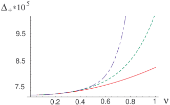
Figure 1: Higher order results for the deviation $\Delta_{+}$ of the index $n_{+}$ from unity as a function of $\nu=\omega/m_{e}$ at fixed background intensity $\epsilon^{2}=0.1$. Full line: second order; short-dashed line: sixth order; long-dashed line: tenth order.

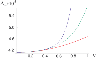
Figure 2: Same as Fig. 1 for $\Delta_{-}$.

As already stated the results of the preceding section indicate strongly that the expansion (66) of the index of refraction is asymptotic both in frequency and intensity. Hence, for both the derivative and weak (external) field expansions we expect factorial growth of the expansion coefficients at large orders.

To test this expectation numerically we expand $\Delta_{\pm}$ in accordance with (66),

$$\Delta_{\pm}(\nu,\epsilon)=\frac{\alpha\epsilon^{2}}{45\pi}\sum_{l\geq 0}\delta_{2l\pm}(\epsilon)\,\nu^{2l}\;,$$ (74)

with $\delta_{2l\pm}$ as given in (67) and form the ratio

$$r_{2l\pm}\equiv\frac{\delta_{2l+2,\pm}}{\epsilon^{2}\,\delta_{2l\pm}}=\frac{c_{2l+2,\pm}(0)}{c_{2l,\pm}(0)}\left[1+O(\alpha)+O(\alpha\epsilon^{2})\right]\;.$$ (75)

The coefficients can (in principle) be determined by expanding the integral representations (38–40) using the auxiliary functions (42) and (43) (see next section). For simple factorial growth, $\delta_{2l}\sim\Gamma(l)$, $r_{2l}$ would depend linearly on $l$.

In what follows we want to ask the question what can be said about the factorial growth without using any knowledge of the special functions (42) and (43). That is, we perform a brute-force derivative expansion before calculating any integrals, trying to extend the method of the previous section to orders as large as possible to gain a maximum of information. The philosophy behind is our expectation that for realistic backgrounds such as laser fields this type of derivative expansion will be one of the main tools when analytical methods are not available. We thus expect our method to provide results complementary to numerical approaches like world-line Monte Carlo [28, 29, 30, 31].

In order to extract the asymptotic behaviour of $\delta_{2l}$ or $r_{2l}$ with high accuracy it is obviously desirable to go to the largest orders possible. Again, this is only feasible with the aid of computer algebra and was performed with an optimised Mathematica routine. Using a standard desktop PC we were able to achieve a maximal order of $\ell=82$. The determination of all 82/2 coefficients for a given value $\epsilon^{2}$ of intensity takes about an hour.

In Fig.s 3 and 4 we have plotted the ratio (75) as a function of order $2l$ for different values of the intensity $\epsilon^{2}$ ranging from 0.1 (subcritical) to 500 (supercritical).

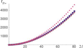
Figure 3: Successive coefficient ratio $r_{2l+}$ as a function of order $2l$ for four different intensities, $\epsilon^{2}=0.1$ ($\fulldiamond$), $\epsilon^{2}=1$ ($\fullstar$), $\epsilon^{2}=100$ ($\fullsquare$) and $\epsilon^{2}=500$ ($\fulltriangle$).

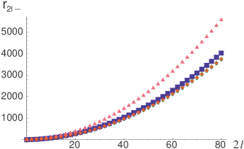
Figure 4: Successive coefficient ratio $r_{2l-}$ as a function of order $2l$ for four different intensities, $\epsilon^{2}=0.1$ ($\fulldiamond$), $\epsilon^{2}=1$ ($\fullstar$), $\epsilon^{2}=100$ ($\fullsquare$) and $\epsilon^{2}=500$ ($\fulltriangle$).

One notes the following: First, the $\epsilon$-dependence of $r_{2l}$ is rather weak as expected from the discussion in the preceding section and the second expression in (75). To recognize corrections to the leading behavior which is independent of $\epsilon$ one has to go to very large intensities and/or orders. For instance, the graphs for $\epsilon^{2}=0.1$ and $\epsilon^{2}=1$ basically are on top of each other. One needs $\epsilon=O(10^{2})$ to see 10% deviations from the graphs with small $\epsilon$ values. This is consistent with the coefficients of $\epsilon^{2}$ in (75) being of order $10^{-3}$, cf. (64) and (65).

Second, and more importantly, the ratio $r_{2l}$ seems to depend quadratically on $l$ which is simply explained by an asymptotic behaviour $r_{2l}\sim\Gamma(2l)$. Let us try to perform a more quantitative analysis. The following general ansatz

$$c_{2l}(0)=\rho^{2l}\Big{[}\Gamma(2l-\sigma)+\tau\,\Gamma(2l-\sigma-1)\Big{]}\;,$$ (76)

which is tailored after examples where exact results are available [26, 32], implies a ratio

$$r_{2l}=\rho^{2}\Big{[}(2l)^{2}+(1-2\sigma)\,2l+\sigma^{2}-\sigma-2\tau\Big{]}\equiv a_{2}\,(2l)^{2}+a_{1}\,2l+a_{0}\;.$$ (77)

Fitting the curves of Fig.s 3 and 4 to quadratic polynomials we find the $a_{i}$ values listed in Table 1.

Table 1: Fitted values for the polynomial coefficients in (77).

	$\epsilon^{2}=0.1$	$\epsilon^{2}=1$	$\epsilon^{2}=100$	$\epsilon^{2}=500$
$a_{2+}$	$0.56256(11)$	$0.56295(35)$	$0.607(11)$	0.8383(38)
$a_{1+}$	$1.6892(29)$	$1.6899(49)$	$1.817(44)$	2.51(42)
$a_{0+}$	$1.691(41)$	$1.693(46)$	$1.69(27)$	1.4(2.5)
$a_{2-}$	$0.562535(27)$	$0.56275(15)$	$0.5865(15)$	0.699(11)
$a_{1-}$	$1.68741(46)$	$1.68795(16)$	$1.7591(21)$	2.10(15)
$a_{0-}$	$1.3926(36)$	$1.3928(70)$	$1.38(13)$	1.25(90)

The errors have been estimated by also fitting higher-order polynomials and monitoring the change in the coefficients. For all fits an extrapolation to $l\to\infty$ has been performed using Laurent series techniques.

Via (77) the values of Table 1 translate into the asymptotic coefficients $\rho$, $\sigma$ and $\tau$ introduced in (76) as listed in Table 2.

Table 2: Numerical values for the polynomial coefficients in (76).

	$\epsilon^{2}=0.1$	$\epsilon^{2}=1$	$\epsilon^{2}=100$	$\epsilon^{2}=500$
$\rho_{+}$	$0.75004(15)$	$0.75030(47)$	$0.779(14)$	$0.9156(42)$
$\sigma_{+}$	$-1.0014(23)$	$-1.009(34)$	$-0.9967(91)$	$-1.00(24)$
$\tau_{+}$	$-0.501(65)$	$-0.502(69)$	$-0.40(35)$	$0.2(2.2)$
$\rho_{-}$	$0.750023(36)$	$0.75017(20)$	$0.7658(20)$	$0.836(13)$
$\sigma_{-}$	$-0.99983(34)$	$-0.99973(26)$	$-0.9997(20)$	$-1.002(84)$
$\tau_{-}$	$-0.2380(52)$	$-0.238(12)$	$-0.18(22)$	$0.11(99)$

One notes that $\rho$ and $\sigma$ are the same for both indices of reflection i.e. $\rho_{+}=\rho_{-}\equiv\rho$ and $\sigma_{+}=\sigma_{-}\equiv\sigma$ while $\tau_{+}\neq\tau_{-}$. Furthermore, $\sigma$ seems to be independent of intensity (unlike $\rho$ and $\tau$). We can even guess the following ‘analytic’ values for $\rho$ and $\sigma$,

$$\rho=3/4\;,\quad\mbox{and}\quad\sigma=-1\;.$$ (78)

For $\epsilon^{2}\lesssim 1$ these values for $\rho$ and $\sigma$ should be quite accurate. Not unexpectedly, the largest errors reside in the subleading coefficients $\tau_{\pm}$. In view of this we refrain from any further guesses and just quote the $\tau$-values of Table 2.

With the coefficients being determined let us plug the ansatz (76) into (74) adopting the approximation (67) so that the expansion parameter becomes $\epsilon\nu$ rather than $\nu$. This should be fine for $\epsilon^{2}\lesssim 1$. As our ansatz (76) is supposed to hold only asymptotically for large orders we cannot expect to describe the low orders accurately. We nevertheless proceed by eliminating the Gamma functions using the integral expression

$$\rho^{z}\,\Gamma(z)=\int_{0}^{\infty}ds\,\frac{e^{-1/\rho s}}{s^{z+1}}\;.$$ (79)

This transforms the required summations over $l$ into geometric series and yields the following integral representation for (74),

$$\Delta_{\pm}(\epsilon,\nu)=N_{\pm}\,\frac{\alpha\epsilon^{2}}{45\pi}\int_{0}^{\infty}ds\,\frac{s}{s^{2}-(\epsilon\nu)^{2}}\left[(\rho s)^{\sigma}+\tau_{\pm}(\rho s)^{\sigma+1}\right]\,e^{-1/\rho s}\;,$$ (80)

where we have allowed for an undetermined scale $N_{\pm}$. As it stands the integral is ambiguous as there are poles on the real axis. The left-hand side may be viewed as originating from the derivative (or $\epsilon\nu$) expansion which has real coefficients. It is therefore tempting to interpret (80) as the following dispersion integral (see e.g. [33], Ch. 18),

$$\mbox{Re}\,\Delta_{\pm}(\epsilon\nu)=N_{\pm}\,\frac{2}{\pi}\;\mathfrak{P}\int_{0}^{\infty}ds\,\frac{s}{s^{2}-(\epsilon\nu)^{2}}\;\mbox{Im}\,\Delta_{\pm}(s)\;,$$ (81)

where the pole ambiguity has been resolved in terms of the Cauchy principal value denoted by $\mathfrak{P}$. The right-hand side contains a ‘nonperturbative imaginary part’ [32],

$$\mbox{Im}\,\Delta_{\pm}(\epsilon\nu)=N_{\pm}\frac{\alpha\epsilon^{2}}{90}\,(\epsilon\nu\rho)^{\sigma}\,(1+\tau_{\pm}\epsilon\nu\rho)\,e^{-1/\epsilon\nu\rho}\;,$$ (82)

i.e. an exponential that cannot be obtained from a perturbative expansion in $\epsilon\nu$. Inserting the universal values (78) and $\tau_{\pm}$ from Table 2 this becomes

$$\mbox{Im}\,\Delta_{\pm}(\epsilon\nu)=N_{\pm}\frac{\alpha\epsilon^{2}}{90}\,\frac{4}{3\epsilon\nu}\,\left(1-\frac{3\epsilon\nu}{4}\left\{0.50\atop 0.24\right\}\right)\,e^{-4/3\epsilon\nu}\;.$$ (83)

Note that the small parameter involved seems to be $3\epsilon\nu/4$.

Summarising we can say that our large-order derivative expansion has provided us with a quantitative formula for the asymptotics of the series which by means of (81) could be turned into a statement about the nonperturbative imaginary part. As already stated, this should be directly related to absorption and pair production. In what follows we will check our findings by an analytic discussion of the integral representations of the eigenvalues $\Pi_{i}$, in particular of (40).

5 Analytic Results

Proceeding analytically is equivalent to analysing the (derivative of the) auxiliary function $f(z)$ introduced in (42). The leading orders for both weak and strong external fields have already been investigated by Narozhnyi [10]. In this section we want to go further and discuss arbitrary large orders in the low-frequency, weak-field expansion of the eigenvalues $\Pi_{i}$. Nevertheless, to keep things manageable we follow Narozhnyi’s example and adopt an approximation that leads to substantial simplifications. Namely, we neglect vacuum modifications in expressions involving the eigenvalues $\Pi_{i}(\lambda,\kappa)$ by setting $n=1$ or, equivalently, $\lambda=0$ in their arguments. From (36) and (37) we thus have the approximate identities

$$\Pi_{0}(\lambda,\kappa^{2}) \simeq \Pi_{0}(0,\kappa^{2})=0\;,$$ (84)

$$\Pi_{\pm}(\lambda,\kappa^{2}) \simeq \Pi_{\pm}(0,\kappa^{2})=-m_{e}^{2}\kappa^{2}P_{\pm}(0,\kappa^{2})\;.$$ (85)

According to (56) we have in the same approximation,

$$\kappa\simeq 2\epsilon\nu\;,$$ (86)

which turns our eigenvalues into functions of the product $\epsilon\nu$ in line with our discussion of the previous section. The upshot of all this is that the dispersion relations (48) simplify drastically so that one is left with the task to determine $P_{\pm}$ in

$$\Delta_{\pm}(\kappa,\lambda)\simeq\Delta_{\pm}(\epsilon\nu)\simeq 2\epsilon^{2}P_{\pm}(\epsilon\nu)\;.$$ (87)

As an aside we remark that according to (33), (34) and (35) Narozhnyi’s approximation is expected to be particularly good if probe and background are perpendicular as $b^{2}$ and hence $\kappa$ are indeed independent of $n$ in this case. The perpendicular setup has recently been suggested as a means to look for ‘vacuum diffraction’ [34].

To evaluate (87) we want to calculate $P_{\pm}$ as a power series in $\epsilon\nu$ using the integral representation (40). From the definition of $\kappa^{2}$ in (35) or (86) and of $z(\lambda,\kappa,x\bar{x})$ in (41) it is clear that an expansion in $\epsilon\nu$ corresponds to determining the large-$z$ asymptotics of

$$f^{\prime}(z)=\pi\,\mbox{Gi}^{\prime}(z)+i\pi\,\mbox{Ai}^{\prime}(z)\;,$$ (88)

which appears in the integrand of (40). Using asymptotic expansions for $\mbox{Ai}(z)$ given in [16] and $\mbox{Gi}(z)$ in [35] one obtains for (88)

$$f^{\prime}(z)=-\frac{1}{z^{2}}-\frac{1}{z^{5}}\sum_{k=0}^{\infty}\frac{g_{k}}{z^{3k}}-\frac{i}{2}\,\pi^{1/2}z^{1/4}e^{-\zeta}\sum_{k=0}^{\infty}(-1)^{k}A_{k}\,\zeta^{-k}\;,$$ (89)

with the abbreviations

$$\zeta \equiv \frac{2}{3}z^{3/2}\;,$$ (90)

$$g_{k} \equiv \frac{(3k+4)\,\Gamma(3k+3)}{3^{k}\,\Gamma(k+1)}\;,$$ (91)

$$A_{k} \equiv -\frac{6k+1}{6k-1}\;\frac{\Gamma(3k+1/2)}{54^{k}\,k!\,\Gamma(k+1/2)}\;.$$ (92)

The expression (89) now has to be plugged in the integral (40). Throughout the subsequent calculations we use Narozhnyi’s approximation which implies

$$z\simeq(\kappa x\bar{x})^{-2/3}\;,\quad\zeta\simeq 2/3\kappa x\bar{x}\;.$$ (93)

In what follows we will separately calculate real and imaginary parts of $P_{\pm}$.

5.1 Calculation of the Real Part

Using (86), (93) and the integral representation of the Beta function,

$$\int_{0}^{1}dx\,x^{n-1}\,\bar{x}^{m-1}=B(n,m)=\frac{\Gamma(n)\,\Gamma(m)}{\Gamma(n+m)}\;,$$ (94)

the real part of $P_{\pm}$ can be obtained in closed form,

$$\mbox{Re}\,P_{\pm}(\kappa)=\frac{\alpha m^{2}}{3\pi}\sum_{l\geq 0}G_{l}\,\kappa^{2l}\Big{\{}2B(2l+2,2l+2)+(1\pm 3)\,B(2l+3,2l+3)\Big{\}}\;.$$ (95)

Here, we have introduced the new expansion coefficients

$$G_{l}\equiv\left\{\begin{array}[]{ll}1\;,&l=0\\ g_{l-1}\;,&l>0\end{array}\right.$$ (96)

The leading term ($l=0$) in the expansion (95) yields for (87)

$$\Delta_{\pm}(\epsilon\nu)=2\epsilon^{2}P_{\pm}(\epsilon\nu)\simeq(11\pm 3)\frac{\alpha\epsilon^{2}}{45\pi}\;,$$ (97)

which reassuringly is consistent with (71).

It is the presence of the Beta functions in (95) that causes factorial growth. To analyse this in the spirit of the previous section we expand the corrections to the indices of refraction according to (66) and (72),

$$\mbox{Re}\,\Delta_{\pm}\equiv 2\epsilon^{2}\mbox{Re}\,P_{\pm}=\frac{\alpha\epsilon^{2}}{45\pi}\sum_{l\geq 0}c_{2l,\pm}(0)(\epsilon\nu)^{2l}\;.$$ (98)

Comparing with (95) we find the coefficient ratios

$$r_{2l\pm}=4\,\frac{G_{l+1}}{G_{l}}\frac{2B(2l+4,2l+4)+(1\pm 3)B(2l+5,2l+5)}{2B(2l+2,2l+2)+(1\pm 3)B(2l+3,2l+3)}\;.$$ (99)

These can be evaluated exactly to give

$$r_{2l+} = \frac{2(6l+13)(3l+4)(3l+2)(2l+3)(l+1)}{(6l+7)(4l+9)(4l+7)}$$ (100)

$$= \frac{9}{16}\,(2l)^{2}+\frac{54}{32}\,2l+\frac{452}{256}-\frac{372}{256}\frac{1}{2l}+O(1/l^{2})\;,$$

$$r_{2l-} = \frac{(6l+14)(3l+2)(2l+3)(l+1)}{(4l+9)(4l+7)}$$ (101)

$$= \frac{9}{16}\,(2l)^{2}+\frac{54}{32}\,2l+\frac{356}{256}-\frac{12}{256}\frac{1}{2l}+O(1/l^{2})\;.$$

Obviously, as the $r_{2l\pm}$ are independent of intensity they cannot describe all curves of Fig.s 3 and 4 which, after all, are intensity dependent. However, we expect good agreement between numerical and analytical values of $r_{2l\pm}$ for small intensities $\epsilon^{2}\lesssim 1$. This is nicely corroborated by the graphs of Fig. 5 where the results for $\epsilon^{2}=0.1$ are on top of each other for all $l$. This near-perfect agreement is due to the fact that upon neglecting the $\epsilon$ dependence of the coefficients (67) (and within Narozhnyi’s approximation) all expansion coefficients are basically factorials, cf. (95).

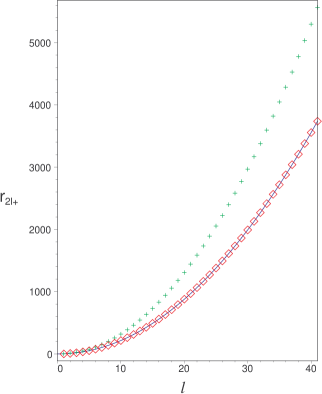
Figure 5: Coefficient ratio $r_{2l+}$ as a function of order $l$. Diamonds: numerical values for $\epsilon^{2}=0.1$; crosses: numerical values for $\epsilon^{2}=500$ (both as in Fig. 3); full line: analytical ratio from (99).

Matching (100) and (101) with (77) we read off the coefficients

$$a_{2} = \frac{9}{16}=0.5625\;,$$ (102)

$$a_{1} = \frac{54}{32}=1.6875\;,$$ (103)

$$a_{0+} = \frac{452}{256}=1.765625\;,$$ (104)

$$a_{0-} = \frac{356}{256}=1.390625\;,$$ (105)

which compare favourably with the entries of Table 1 for $\epsilon^{2}\lesssim 1$. The $a_{i}$ translate exactly into the asymptotic parameters $\rho=3/4$ and $\sigma=-1$ we had guessed in (78) while the $\tau$-parameters become

$$\tau_{+} = -\frac{41}{72}=-0.5694\;,$$ (106)

$$\tau_{-} = -\frac{17}{72}=-0.2361\;.$$ (107)

Again, these agree satisfactorily with the entries of Table 2 for small $\epsilon$, in particular for subscript ‘minus’.

It remains to rewrite our nonperturbative imaginary part (83) by replacing the numerical $\tau_{\pm}$ by their analytic counterparts just obtained,

$$\mbox{Im}\,\Delta_{\pm}(\epsilon\nu)=N_{\pm}\frac{\alpha\epsilon^{2}}{90}\,\frac{4}{3\epsilon\nu}\,\left(1-\frac{3\epsilon\nu}{4}\frac{29\pm 12}{72}\right)\,e^{-4/3\epsilon\nu}\;.$$ (108)

Let us finally try to check this by a direct calculation of the imaginary part.

5.2 Calculation of the Imaginary Part

The determination of the imaginary part of $P_{\pm}$ is more involved as the integrand (40) contains an exponential that cannot be expanded in powers of $x\bar{x}$. Explicitly, the integrand is of the form

$$e^{-\zeta}\,(x\bar{x})^{n}\simeq\exp(-2/3\kappa x\bar{x})\,(x\bar{x})^{n}\;,$$ (109)

which is to be integrated from 0 to 1. In order to proceed analytically we note that the product $x\bar{x}$ is peaked at the value 1/4. Thus, it seems feasible to perform the integral via saddle point approximation which results in the formula

$$I(a,b)\equiv\int_{0}^{1}dx\,e^{-ax\bar{x}}(x\bar{x})^{b}\simeq\left(\frac{\pi}{16a+4b}\right)^{1/2}4^{-b}\,e^{-4a}\;.$$ (110)

Here, the first prefactor has been obtained by extending the integration to the whole real axis in order to have a Gaussian integral. In our case, the parameters $a$ and $b$ are given by

$$a=2/3\kappa\simeq 1/3\epsilon\nu\quad\mbox{and}\quad b=k\pm 1/2\;,\;k=0,1,2,\ldots\;.$$ (111)

Comparison with a numerical evaluation for $k=0\ldots 5$ shows that the error of the approximation is about 10% for $a=1$, 1% for $a=5$ and $0.1\%$ for $a=10$. Hence, for large $a$ (which we have) the formula (110) should work very well.

Having gained sufficient confidence in our saddle point approximation we rewrite the imaginary part of (40) using (89),

$$\mbox{Im}\,P_{\pm}\simeq\frac{\alpha}{6\pi^{1/2}}\,\kappa^{-3/2}\sum_{k\geq 0}(-1)^{k}\,A_{k}\,\Big{\{}2\,I(a,k-1/2)+(1\pm 3)\,I(a,k+1/2)\Big{\}}\;,$$ (112)

with $A_{k}$ as defined in (92). Employing our integration formula (110) we find

$$\mbox{Im}\,P_{\pm}\simeq\frac{\alpha}{24}\,\sqrt{\frac{3}{2}}\,\frac{1}{\kappa}\,e^{-8/3\kappa}\,\sum_{k\geq 0}B_{k\pm}\left(-\frac{3\kappa}{8}\right)^{k}\;,$$ (113)

where the new expansion coefficients are given by the somewhat lengthy expression

$$B_{k\pm}\equiv A_{k}\,\left\{\frac{9\pm 3}{4}+\frac{72k}{(6k-7)(6k+1)}\left[\frac{9\pm 3}{4}(k-1)+\frac{-7\pm 3}{8}\right]\right\}\;.$$ (114)

Admittedly, this is not too illuminating so we evaluate the series (113) to order $\kappa^{2}$ or $(\epsilon\nu)^{2}$ and use (87) to determine

$$\mbox{Im}\,\Delta_{\pm}\simeq N_{\pm,\mathrm{sp}}\,\frac{\alpha\epsilon^{2}}{90}\,\frac{4}{3\epsilon\nu}\,e^{-4/3\epsilon\nu}\,\left\{1+\frac{25\mp 12}{72}\frac{3\epsilon\nu}{4}+\frac{265\mp 168}{2\times 72^{2}}\left(\frac{3\epsilon\nu}{4}\right)^{2}\ldots\right\}.$$ (115)

In the above we have introduced the saddle point normalisation factor

$$N_{\pm,\mathrm{sp}}\equiv(3\pm 1)\frac{45}{32}\sqrt{\frac{3}{2}}\;.$$ (116)

We refrain from identifying this with the analogous factor in (108) as the approximation schemes involved do not allow for a direct comparison of the normalisation. The latter will be fixed in a moment by means of the dispersion relation (81).

Putting these niceties aside we stress that we find perfect agreement between (108) and (115) concerning the LO dependence on powers of $\epsilon\nu$ and the nonperturbative exponential. The only discrepancy resides in the $\tau$-coefficients multiplying the subleading terms of order $\epsilon\nu$. In view of the fairly different approximations employed this is probably not too surprising.

6 Discussion and Conclusion

With the consequences of our large-order analysis confirmed analytically we can go even one step further. We can use the Kramers-Kronig relation (81) to actually define the real part of the indices of refraction nonperturbatively, i.e. without relying on the derivative expansion. To this end we take the leading order of the imaginary part (108) or (115) as a model by writing

$$\mbox{Im}\,\Delta_{\pm}(\epsilon,\nu)=N_{\pm}\,\frac{\alpha\epsilon^{2}}{90}\,\frac{4}{3\epsilon\nu}\,e^{-4/3\epsilon\nu}\;.$$ (117)

Plugging this into the the dispersion relation (81) we can actually perform the principal value integral analytically with the result

$$\mbox{Re}\,\Delta_{\pm}=N_{\pm}\,\frac{\alpha\epsilon^{2}}{90\pi}\,\frac{4}{3\epsilon\nu}\Big{\{}\mbox{Ei}(4/3\epsilon\nu)\,e^{-4/3\epsilon\nu}-\mbox{Ei}(-4/3\epsilon\nu)\,e^{4/3\epsilon\nu}\Big{\}}\;.$$ (118)

Matching the perturbative small-$\epsilon\nu$ behaviour fixes the normalisation to be

$$N_{\pm}=11\pm 3\;.$$ (119)

Interestingly, in (118) exponential integrals Ei appear multiplied by exponentials, constituting a paradigm example of functions displaying factorial growth expansion coefficients. With the real part thus determined we summarise our findings in Fig. 6 which shows both real and imaginary part of $\Delta_{+}$ as a function of frequency $\nu$ for fixed $\epsilon^{2}=0.1$. We have added the series expansion to second order (the full line of Fig.1) which coincides well with the exact real part for small $\nu$ where the factorial growth is not visible yet.

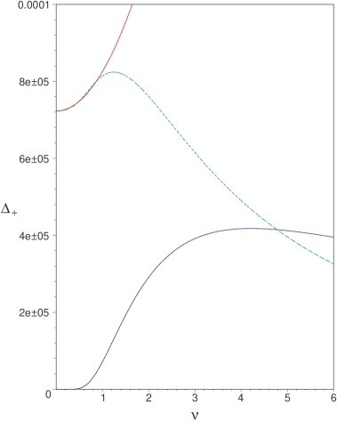
Figure 6: Real and imaginary part of the deviation $\Delta_{+}$ of the index $n_{+}$ from unity (dashed and lower full curve, respectively). The upper full curve bending upwards is the series expansion of $\Delta_{+}$ to second order (same curve as in Fig.1).

The graph for $\Delta_{-}$ looks almost identical with a slight shift in the vertical scale due to the difference in normalisation. Hence, we refrain from producing an extra plot.

By construction, the real and imaginary parts of $\Delta$ (thus also of $n=1+\Delta$) are related by the Kramers-Kronig relation (81) with $\mbox{Im}\,n\neq 0$ signalling absorption, i.e. pair production. By looking at Fig. 6 we see that the latter sets in roughly at the critical value of $\nu=1$. Here, $\mbox{Re}\,n$ attains its maximum and decreases for $\nu\gtrsim 1$ while $\mbox{Im}\,n$ increases. Mathematically, we may state

$$\begin{array}[]{lll}\displaystyle\frac{\partial\mbox{Re}\,n_{\pm}}{\partial\omega}>0&\mbox{for}\;\omega\ll m_{e}\;,&\quad\mbox{(normal dispersion)}\\[10.0pt] \displaystyle\frac{\partial\mbox{Re}\,n_{\pm}}{\partial\omega}<0&\mbox{for}\;\omega\gtrsim m_{e}\;,&\quad\mbox{(anomalous dispersion)}\end{array}$$ (120)

where we have reinstated physical units (recall that $\omega$ is the probe frequency). We conclude that it is a consequence of the Kramers-Kronig relations based on the fundamental principle of causality that absorption is intimately connected to anomalous dispersion.

The physics involved can be wrapped up as follows. We have analysed the influence of crossed background fields on the propagation of light (e.g. laser beams). Using exact integral representations for the eigenvalues of the polarisation tensor we found that to all orders in probe frequency and background intensity there is birefringence of the vacuum induced by the crossed background fields. The effect can be described in terms of background dependent effective metrics $h_{\pm}^{\mu\nu}$ implying dispersion relations $h_{\pm}^{\mu\nu}k_{\mu}k_{\nu}=0$ which describe distorted light-cones. Solving for the indices of refraction $n_{\pm}$ one finds that they are frequency dependent, starting out with normal dispersion. At critical energy and intensity anomalous dispersion sets in together with absorption due to pair production.

At present an experiment is being designed that plans to measure vacuum birefringence using a high power laser background probed by x-ray beams [6]. The experiment is quite demanding as one has to measure ellipticity signals with a sensitivity at the order of $10^{-11}$ for presently available probes and lasers. As the signal is proportional to $\nu^{2}\epsilon^{4}$ it may be readily enhanced by increasing probe frequency and background intensity. Within the next few years one expects a reduction of the required sensitivity down to $10^{-4}$. Normal dispersion is an NLO effect, hence implies a signal of order $\nu^{4}\epsilon^{4}$ requiring a sensitivity of $10^{-8}$ within the envisaged scenario. This is still within the theoretical limits of measurability [36]. Pair production shows up in terms of a nonvanishing imaginary part or as anomalous dispersion of the real part. To become observable both effects require parameters $\nu$ and $\epsilon$ close to their critical values. For instance, if $\epsilon\simeq 10^{-2}$ then $\mbox{Im}\Delta\simeq 10^{-11}$ for $\nu\simeq 0.8$. Even these moderate values cannot be attained at present so that it is presumably more reasonable to look for positrons rather than optical signals to detect pair production.

From a theorist’s point of view one should also consider two-loop corrections and the influence of nonconstant backgrounds. The two-loop corrections to the Heisenberg-Euler Lagrangian (cf. App. A) have been calculated by Ritus [37]. They amount to a replacement of the LO coefficients of (71) according to

$$\left\{14\atop 8\right\}\to\left\{{14\;(1+1315\alpha/252\pi)}\atop{8\;(1+40\alpha/9\pi)}\right\}\;.$$ (121)

These are both one-percent corrections to the LO=$O(\nu^{0})$ behaviour in (71).

Regarding nonconstant backgrounds it is possible to slightly relax the crossed-field assumption in a perfectly controlled manner. Laser beams may be more realistically described as Gaussian beams rather than plane waves. The former have a Gaussian profile in transverse direction of ‘waist size’ $w_{0}$ and a Lorenz profile in the longitudinal direction characterized by the ‘Rayleigh length’ $z_{0}$. One can form the small dimensionless parameter $\triangle\equiv w_{0}/2z_{0}\ll 1$ [38] which describes the deviation from the crossed-field limit corresponding to $\triangle=0$. Naturally, one expects that there will be $O(\triangle)$-corrections to the results presented here.

It is this context of nonconstant backgrounds where the intuition gained in this paper is expected to pay off. In this more realistic case, we cannot hope to have any exact analytical results available. Thus it is important to know both the region of validity and the limitations of derivative and weak-field expansions. From our results they are both expected to break down if the product of frequency squared and intensity becomes $\omega^{2}I=O(m_{e}^{6}/e^{2})$, or, in dimensionless units, $\epsilon^{2}\nu^{2}=O(1)$ (see Fig. 6). With the present values of $\epsilon^{2}\nu^{2}\simeq 10^{-13}$ and those expected in the near future ($\epsilon^{2}\nu^{2}\simeq 10^{-10}$), however, one is definitely on the safe side where (asymptotic) expansion methods make perfect sense.

Appendix A Heisenberg-Euler Analysis

In this appendix we will check our LO results (59) and (60) in an independent manner by using the Heisenberg-Euler (HE) effective Lagrangian [39, 40]. This is the LO in the derivative expansion of the effective action (5) but contains all orders in the intensity. It has the well-known proper-time representation [4] (we follow the nice review [9])

$$\delta\mathscr{L}=\!-\frac{1}{8\pi^{2}}\int\limits_{0}^{\infty}\frac{ds}{s}\,e^{-seE_{c}}\bigg{\{}\frac{e^{2}\mathfrak{a}\mathfrak{b}s^{2}}{\tanh(e\mathfrak{b}s)\tan(e\mathfrak{a}s)}-1-\frac{e^{2}s^{2}}{3}(\mathfrak{a}^{2}-\mathfrak{b}^{2})\bigg{\}},$$ (122)

and is exact for constant fields but remains approximately valid for photon frequencies small compared to the electron mass as in (12). The quantities $\pm i\mathfrak{a}$ and $\pm\mathfrak{b}$ are the eigenvalues of the constant matrix

$$G_{\mu\nu}\equiv F_{\mu\nu}+f_{\mu\nu}\;,$$ (123)

consisting of both background and probe field. They are related to the standard scalar and pseudoscalar invariants defined in (22) and (23) via

$$\mathfrak{a}^{2}-\mathfrak{b}^{2} = -\frac{1}{2}G_{\mu\nu}G^{\mu\nu}\equiv 2\mathscr{S}\;,$$ (124)

$$\mathfrak{a}\mathfrak{b} = -\frac{1}{4}G_{\mu\nu}\tilde{G}^{\mu\nu}\equiv\mathscr{P}\ ;$$ (125)

Note that in this appendix the invariants $\mathscr{S}$ and $\mathscr{P}$ denote the contribution of both background and fluctuation, cf. (123), and thus are nonvanishing. The representation (122) contains all orders in the field $G_{\mu\nu}$. Low intensities allow for a weak-field expansion the first two orders of which are

$$\delta\mathscr{L}=\frac{\alpha^{2}}{m_{e}^{4}}\left(\frac{8}{45}\mathscr{S}^{2}+\frac{14}{45}\mathscr{P}^{2}\right)+\frac{\alpha^{3}}{m_{e}^{8}}\left(\frac{256\pi}{315}\mathscr{S}^{3}+\frac{416\pi}{315}\mathscr{S}\mathscr{P}^{2}\right)\;.$$ (126)

It is worth to point out that exactly the same numerical coefficients appear as in (71).

For what follows it is useful to write the LO of (126) as

$$\delta\mathscr{L}=\frac{1}{2}\gamma_{-}\mathscr{S}^{2}+\frac{1}{2}\gamma_{+}\mathscr{P}^{2}+O(\alpha^{3})\;,$$ (127)

with the couplings $\gamma_{\pm}$ given by

$$\gamma_{+}\equiv 7\xi\;,\quad\gamma_{-}\equiv 4\xi\;,\quad\xi\equiv\frac{\alpha}{45\pi}\frac{1}{E_{c}^{2}}\;.$$ (128)

To approximate the polarisation tensor $\Pi^{\mu\nu}$ we start from (126), decompose into background $F$ and probe $f$ according to (123) and expand the HE action, $\delta S=\int d^{4}x\,\delta\mathscr{L}$, to second order in the probe field $f$,

$$\delta S[F,f]={\textstyle\frac{1}{8}}\left(f_{\alpha\beta},\Omega^{\alpha\beta\mu\nu}\,f_{\mu\nu}\right)\;.$$ (129)

The tensor $\Omega^{\alpha\beta\mu\nu}$ is proportional to the second derivative of $\delta\mathscr{L}$,

$$\Omega^{\alpha\beta\mu\nu}\equiv 4\left.\frac{\partial^{2}(\delta\mathscr{L})}{\partial f_{\alpha\beta}\,\partial f_{\mu\nu}}\right|_{f=0}\;.$$ (130)

So far we have not exploited the fact that our background consists of crossed fields. Note that the derivative in (130) is evaluated right at the background. It is easy to see that enormous simplifications arise in the crossed-field case due to the vanishing of the background invariants. The generic term in the HE Lagrangian is of the form $\mathscr{S}^{n}\mathscr{P}^{2m}$ (as odd powers of $\mathscr{P}$ are forbidden by CP invariance) with $n$ and $m$ integers. Taking the two derivatives in (130) at $f=0$ one will always end up with (vanishing) powers of $\mathscr{S}$ and $\mathscr{P}$ unless $n$ and $m$ are sufficiently small. The only surviving cases turn out to be the Maxwell term, $(n=1$, $m=0$), and the LO (127) with $n=2$, $m=0$ and $n=0$, $m=1$. Thus, for crossed fields, the effective Lagrangian (122) gets truncated after the LO $\alpha^{2}/m_{e}^{4}$. In other words, the LO describes the exact dependence on intensity for crossed-field background! In view of these considerations the tensor $\Omega^{\mu\nu\alpha\beta}$ simplifies to

$$\Omega^{\mu\nu\alpha\beta}=\gamma_{-}F^{\alpha\beta}F^{\mu\nu}+\gamma_{+}\tilde{F}^{\alpha\beta}\tilde{F}^{\mu\nu}\;.$$ (131)

Note that it is symmetric upon exchanging $(\mu\nu)\leftrightarrow(\alpha\beta)$ and antisymmetric both in $\mu$ and $\nu$ as well as $\alpha$ and $\beta$.

In momentum space the polarisation tensor $\Pi^{\mu\nu}$ is then given by contracting (131) twice with the wave vector $k$ associated with the probe field $f_{\mu\nu}$,

$$\Pi^{\mu\nu}(k)\equiv\Omega^{\mu\alpha\nu\beta}k_{\alpha}k_{\beta}=\gamma_{-}\,b^{\mu}b^{\nu}+\gamma_{+}\,\tilde{b}^{\mu}\tilde{b}^{\nu}\;.$$ (132)

To LO in $k^{2}$ this coincides with (21) as it should, the nonvanishing eigenvalues being given by $\Pi_{\pm}=\gamma_{\pm}b^{2}(k)$. They imply the dispersion relations,

$$k^{2}-\gamma_{\pm}b^{2}(k)=0\;$$ (133)

and effective metrics

$$h_{\pm}^{\mu\nu}=g^{\mu\nu}+\gamma_{\pm}T^{\mu\nu}\;.$$ (134)

Introducing the index $n$ of refraction according to (4) the dispersion relations (133) and (134) become four quadratic equations for $n$. Demanding $n=1$ for $\gamma_{\pm}=0$ singles out two of them. These are conveniently written in terms of the abbreviations (29-31),

$$n_{\pm}=\frac{1}{1-\gamma_{\pm}(\mathcal{H}-\mathcal{H}_{k})}\left\{\sqrt{1+\gamma_{\pm}\mathcal{H}_{k}-\gamma_{\pm}^{2}\left[\mathcal{H}^{2}-(\mbox{\bf k}\cdot\mbox{\boldmath$S$})^{2}-\mathcal{H}\mathcal{H}_{k}\right]}-\gamma_{\pm}\mbox{\bf k}\cdot\mbox{\boldmath$S$}\right\}\;$$ (135)

and have the small-$\gamma_{\pm}$ expansion,

$$n_{\pm} = 1+\gamma_{\pm}\left(\mathcal{H}-\mbox{\bf k}\cdot\mbox{\boldmath$S$}-\mathcal{H}_{k}/2\right)+\frac{1}{2}\gamma_{\pm}^{2}\left[(\mathcal{H}-\mbox{\bf k}\cdot\mbox{\boldmath$S$}-\mathcal{H}_{k})^{2}-\mathcal{H}_{k}/2\right]+\ldots\;.$$ (136)

For a head-on collision of probe and background (135) yields the simple expression

$$n_{\pm}=\frac{1+\gamma_{\pm}\,I}{1-\gamma_{\pm}\,I}=1+\frac{2\gamma_{\pm}I}{1-\gamma_{\pm}I}\equiv 1+\Delta_{\pm}\;,$$ (137)

which is exact to all orders in the intensity $I$. Noting that

$$\gamma_{\pm}I=\frac{11\pm 3}{2}\frac{\alpha\epsilon^{2}}{45\pi}\;,$$ (138)

the result (137) coincides with (59) and (60).

References

References

• [1] T. Tajima and G. Mourou. Zettawatt-exawatt lasers and their applications in ultrastrong-field physics. Phys. Rev. ST Accel. Beams, 5:031301, 2002.
• [2] J. Hein, S. Podleska, M. Siebold, M. Hellwing, R. Bödefeld, R. Sauerbrey, D. Ehrt, and W. Winzer. Diode-pumped chirped pulse amplification to the joule level. Appl. Phys. B, 79:419, 2004.
• [3] see e.g. the XFEL-STI interim report at http://xfel.desy.de/
• [4] J. Schwinger. On gauge invariance and vacuum polarization. Phys. Rev., 82:664, 1951.
• [5] F. Sauter. Über das Verhalten eines Elektrons im homogenen elektrischen Feld nach der relativistischen Theorie Diracs. Z. Phys., 69:742, 1931.
• [6] T. Heinzl, B. Liesfeld, K. U. Amthor, H. Schwoerer, R. Sauerbrey and A. Wipf. On the observation of vacuum birefringence. Preprint hep-ph/0601076, 2006.
• [7] E. Brezin and C. Itzykson. Polarization phenomena in vacuum nonlinear electrodynamics. Phys. Rev. D, 3:618, 1970.
• [8] W. Dittrich and H. Gies. Probing the quantum vacuum, volume 166 of Springer Tracts Mod. Phys. Springer, Berlin, 2000.
• [9] Gerald V. Dunne. Heisenberg-Euler effective Lagrangians: Basics and extensions. Preprint hep-th/0406216, 2004.
• [10] N.B. Narozhnyi. Propagation of plane electromagnetic waves in a constant field. Zh. Eksp. Teor. Fiz., 55:714–721, 1968. [Sov. Phys. JETP 28, 371 (1969)].
• [11] V.I. Ritus. Radiative corrections in quantum electrodynamics with intense field and their analytical properties. Ann. Phys., 69:555, 1972.
• [12] H. Schwoerer, B. Liesfeld, H.-P. Schlenvoigt, K-U. Amthor and R. Sauerbrey. Thomson-backscattered x-rays from laser-accelerated electrons. Phys. Rev. Lett., 96:014802, 2006.
• [13] A. Ringwald. Boiling the vacuum with an X-ray free electron laser. Preprint hep-ph/0304139, 2003.
• [14] Ian Affleck and Leonid Kruglyak. Photon splitting in a plane wave field. Phys. Rev. Lett., 59:1065, 1987.
• [15] Z. Białynicka-Birula and I. Białynicki-Birula. Nonlinear effects in quantum electrodynamics. photon propagation and photon splitting in an external field. Phys. Rev. D, 2:2341, 1970.
• [16] M. Abramowitz and I.A. Stegun (ed.s). Handbook of Mathematical Functions (with Formulas, Graphs, and Mathematical Tables). 9th printing, Dover, New York, 1970.
• [17] http://dlmf.nist.gov/.
• [18] M.E. Peskin and D.V. Schroeder. An Introduction to Quantum Field Theory. Addison-Wesley, Reading, MA, 1995.
• [19] Stefano Liberati, Sebastiano Sonego, and Matt Visser. Scharnhorst effect at oblique incidence. Phys. Rev., D63:085003, 2001.
• [20] E. Zavattini et al. Experimental observation of optical rotation generated in vacuum by a magnetic field. Preprint hep-ex/0507107, 2005.
• [21] J. Toll. The Dispersion Relation for Light and its Application to Problems Involving Electron Pairs. PhD thesis, Princeton, 1952
• [22] K.T. McDonald. Proposal for experimental studies of nonlinear Quantum Electrodynamics. Preprint DOE/ER/3072-38, 1986. Available as http://www.hep.princeton.edu/ mcdonald/e144/prop.pdf.
• [23] R. Baier and P. Breitenlohner. Acta Phys. Austriaca, 25:212, 1967.
• [24] R. Baier and P. Breitenlohner. Nuovo Cim. B, 47:117, 1967.
• [25] Stephen L. Adler. Photon splitting and photon dispersion in a strong magnetic field. Annals Phys., 67:599–647, 1971.
• [26] Gerald V. Dunne and Theodore M. Hall. Borel summation of the derivative expansion and effective actions. Phys. Rev., D60:065002, 1999.
• [27] Paul E. L. Rakow. Stochastic perturbation theory and the gluon condensate. PoS, LAT2005:284, 2005.
• [28] H. Gies and K. Langfeld. Loops and loop clouds: A numerical approach to the worldline formalism in QED. Int. J. Mod. Phys. A, 17:966, 2002.
• [29] H. Gies and K. Langfeld. Quantum diffusion of magnetic fields in a numerical worldline approach. Nucl. Phys. B, 613:353, 2001.
• [30] H. Gies, J. Sanchez-Guillen and R. A. Vazquez. Quantum effective actions from nonperturbative worldline dynamics. JHEP, 0508:067, 2005.
• [31] H. Gies and K. Klingmüller. Pair production in inhomogeneous fields. Phys. Rev. D, 72:065001, 2005.
• [32] Gerald V. Dunne. Perturbative-nonperturbative connection in quantum mechanics and field theory. Preprint hep-th/0207046, 2002.
• [33] J.D. Bjorken and S.D. Drell, Relativistic Quantum Field Theory. McGraw-Hill, New York, 1965.
• [34] A. Di Piazza, K. Z. Hatsagortsyan and C. H. Keitel, Light diffraction by a strong standing electromagnetic wave. Preprint hep-ph/0602039, 2006.
• [35] A. Gil, J. Segura and N.N. Temme. GIZ, HIZ: Two Fortran 77 routines for the computation of complex Scorer functions”. ACM Trans. Math. Soft., 28:436, 2002.
• [36] E.E. Alp, W. Sturhahn, and T.S. Toellner. Polarizer-analyzer optics. Hyperfine Interactions, 125:45, 2000.
• [37] V.I. Ritus. Sov. Phys. JETP, 42:774, 1976.
• [38] S.S. Bulanov, N.B. Narozhny, V.D. Mur, and V.S. Popov. On $e^{+}e^{-}$-pair production by a focused laser pulse in vacuum. Phys. Lett. A, 330:1, 2004.
• [39] W. Heisenberg and H. Euler. Folgerungen aus der Diracschen Theorie des Positrons. Z. Phys., 98:714–732, 1936.
• [40] V. Weisskopf. Über die Elektrodynamik des Vakuums auf Grund der Quantentheorie des Elektrons. K. Dan. Vidensk. Selsk. Mat. Fys. Medd., 14:6, 1936. Reprinted in Quantum Electrodynamics, J. Schwinger, ed., Dover, New York 1958.