OCU-PHYS 247

hep-th/0605129

Explicit Toric Metric on
Resolved Calabi-Yau Cone

Takeshi Oota¹ and Yukinori Yasui²

¹Osaka City University, Advanced Mathematical Institute (OCAMI)
3-3-138 Sugimoto, Sumiyoshi, Osaka 558-8585, Japan
²Department of Mathematics and Physics, Graduate School of Science,
Osaka City University
3-3-138 Sugimoto, Sumiyoshi, Osaka 558-8585, Japan

We present an explicit non-singular complete toric Calabi-Yau metric using the local solution recently found by Chen, Lü and Pope. This metric gives a new supergravity solution representing D3-branes.

D3-branes on the tip of toric Calabi-Yau cones have been extensively studied in connection with the AdS/CFT correspondence [1]. It is natural to consider the deformations of cone metrics in order to explore non-conformal theories [2, 3, 4, 5, 6, 7].

In this letter, we study a Calabi-Yau metric,  i.e. Ricci-flat Kähler metric, constructed as the BPS limit of the six dimensional Euclideanised Kerr-NUT-AdS black hole metric [8]. In the black hole with equal angular momenta, the corresponding Calabi-Yau metric is of the form

$$g = \frac{(1-x)(1-z)}{3}(d\theta^{2}+\sin^{2}\theta d\phi^{2})+\frac{(1-x)(x-z)}{f(x)}dx^{2}+\frac{(1-z)(z-x)}{h(z)}dz^{2}$$

$$+ \frac{f(x)}{9(1-x)(x-z)}(d\psi-\cos\theta d\phi+z(d\beta+\cos\theta d\phi))^{2}$$

$$+ \frac{h(z)}{9(1-z)(z-x)}(d\psi-\cos\theta d\phi+x(d\beta+\cos\theta d\phi))^{2},$$

where

$$f(x)=2x^{3}-3x^{2}+a,~{}~{}h(z)=2z^{3}-3z^{2}+b$$ (2)

with two parameters $a$ and $b$. We assume that the roots $x_{i}$ ($i=1,2,3$) of $f(x)=0$ are all distinct and real, and further they are ordered as $z_{1}<x_{1}<x_{2}<x_{3}$ for the smallest real root $z_{1}$ of $h(z)=0$. In order to avoid a curvature singularity we take the coordinates $x$ and $z$ to lie in the region $z\leq z_{1}<x_{1}\leq x\leq x_{2}<1$. Indeed, it is easy to see that such a singularity appears at $z=x$.

For $r\to\infty~{}(z=-r^{2}/2)$ , the metric tends to a cone metric $dr^{2}+r^{2}\bar{g}$, where

$$\bar{g} = \frac{1-x}{6}(d\theta^{2}+\sin^{2}\theta d\phi^{2})+\frac{1-x}{2f(x)}dx^{2}+\frac{f(x)}{18(1-x)}(d\beta+\cos\theta d\phi)^{2}$$

$$+ \frac{1}{9}(d\psi-\cos\theta d\phi+x(d\beta+\cos\theta d\phi))^{2}.$$

This metric yields the Sasaki-Einstein metric $Y^{p,q}$ when we impose a suitable condition for the parameter $a$ [9].

Next let us look at the geometry near $z=z_{1}$. We introduce new coordinates given by

$$\varphi_{1}=-\frac{1}{2}(\psi-z_{1}\beta),~{}~{}\varphi_{2}=\frac{1}{1-z_{1}}(\psi+z_{1}\beta),~{}~{}\varphi_{3}=\phi.$$ (4)

Then the metric behaves as

$$g\simeq du^{2}+u^{2}d\varphi_{1}^{2}+g^{(4)},$$ (5)

where $u^{2}=2(z_{1}-x)(z_{1}-z)/(3z_{1})$. Therefore, the periodicity of $\varphi_{1}$ should be $2\pi$ in order to avoid an orbifold singularity. The four dimensional Kähler metric $g^{(4)}$ is given by

$$g^{(4)} = \frac{(1-x)(1-z_{1})}{3}(d\theta^{2}+\sin^{2}\theta d\varphi_{3}^{2})+\frac{(1-x)(x-z_{1})}{f(x)}dx^{2}$$

$$+ \frac{(1-z_{1})^{2}f(x)}{9(1-x)(x-z_{1})}(d\varphi_{2}-\cos\theta d\varphi_{3})^{2}.$$

We now argue that by taking the special parameters $a=(1/2)-(1/32)\sqrt{13}$ which corresponds to $Y^{2,1}$, and $b=(1/4)(137+37\sqrt{13})$, the four dimensional space with metric $g^{(4)}$ is a non-trivial $S^{2}$-bundle over $S^{2}$, i.e. the first del Pezzo surface $dP_{1}$. To see this, introduce a radial coordinate $y^{2}=2(x_{i}-z_{1})\mid x-x_{i}\mid/\mid 3x_{i}\mid$ on the $(x,\varphi_{2})$-fibre space defined by fixing the $S^{2}$ coordinates $\theta$ and $\varphi_{3}$ in (S0.Ex4). Then, the fibre metric near boundary $x=x_{i}$ $(i=1,2)$ is written as

$$dy^{2}+\left(\frac{x_{i}(1-z_{1})}{x_{i}-z_{1}}\right)^{2}y^{2}d\varphi_{2}^{2}.$$ (7)

Using the values of $a$ and $b$, we have

$$x_{1}=\frac{1}{8}(1-\sqrt{13}),~{}~{}x_{2}=\frac{1}{8}(7-\sqrt{13}),~{}~{}z_{1}=-\frac{1}{2}(2+\sqrt{13}),$$ (8)

and then $x_{i}(1-z_{1})/(x_{i}-z_{1})=\pm 1/2$. The apparent singularities at $x=x_{i}$ can be avoided by choosing the periodicity of $\varphi_{2}$ to be $4\pi$. Thus, the $(x,\varphi_{2})$-fibre space is topologically $S^{2}$. On the other hand, fixing the coordinate $x$ in (S0.Ex4), we obtain a principal $U(1)$-bundle over $S^{2}$ with the Chern number

$$\frac{1}{4\pi}\int_{S^{2}}d(-\cos\theta d\varphi_{3})=1.$$ (9)

The metric $g^{(4)}$ can be regarded as a metric on the associated $S^{2}$-bundle of the principal $U(1)$-bundle. The associated bundle is non-trivial since the Chern number is odd, and hence the total space is the $dP_{1}$.

Let us describe the Calabi-Yau metric (S0.Ex2) from the point of view of toric geometry. The metric has an isometry $T^{3}$, locally generated by the Killing vector fields, $\partial/\partial\psi,~{}\partial/\partial\phi$ and $\partial/\partial\beta$. The symplectic (Kähler) form $\omega$ is given by

$$\omega=\frac{1}{3}\Bigl{(}d\psi\wedge d(x+z)+d\phi\wedge d((1-x)(1-z)\cos\theta)+d\beta\wedge d(xz)\Bigr{)}.$$ (10)

Using the following generators of the $T^{3}$ action [10],

$$\frac{\partial}{\partial\phi_{1}} = \frac{\partial}{\partial\psi}+\frac{\partial}{\partial\phi}-\frac{\partial}{\partial\beta},$$ (11)

$$\frac{\partial}{\partial\phi_{2}} = \frac{\partial}{\partial\phi}+3\ell\frac{\partial}{\partial\beta},$$ (12)

$$\frac{\partial}{\partial\phi_{3}} = -6\ell\frac{\partial}{\partial\beta},$$ (13)

one has Darboux coordinates $(\xi^{1},~{}\xi^{2},~{}\xi^{3})$ on which the symplectic form takes the standard form $\omega=d\xi^{i}\wedge d\phi_{i}$:

$$\xi^{1} = \frac{1}{3}(1-x)(1-z)(1-\cos\theta),$$ (14)

$$\xi^{2} = -\frac{\ell}{2}(2xz+1)-\frac{1}{3}(1-x)(1-z)\cos\theta,$$ (15)

$$\xi^{3} = \ell(2xz+1)$$ (16)

with $\ell^{-1}=-5+2\sqrt{13}$. For the range of variables: $0\leq\theta\leq\pi,x_{1}\leq x\leq x_{2},~{}z\leq z_{1}$, where $x_{1},x_{2}$ and $z_{1}$ are given by (8), we find the Delzant polytope (see Fig.1)

$$P=\{\xi=(\xi^{1},\xi^{2},\xi^{3})\in\mathbb{R}^{3}\mid(\xi,v_{a})\geq\lambda_{a},\,a=1,2,\dots,5\}.$$ (17)

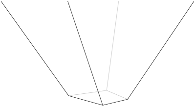
Figure 1: Delzant polytope $P$

Here, each $v_{a}$ is a primitive element of the lattice $\mathbb{Z}^{3}\subset\mathbb{R}^{3}$ and an inward-pointing normal vector to the two dimensional face of $P$. Explicitly, the set of five vectors $v_{a}=(1,w_{a})$ can be chosen as (see Fig. 2)

$$w_{1}=(-1,-2),\ \ w_{2}=(0,0),\ \ w_{3}=(-1,0),\ \ w_{4}=(-2,-1),\ \ w_{5}=(-1,-1).$$ (18)

Figure 2: Toric diagram

The constants $\lambda_{a}$ are given by

$$\lambda_{1}=\frac{1}{72}(1-5\sqrt{13}),\qquad\lambda_{3}=\frac{1}{216}(29+17\sqrt{13}),\qquad\lambda_{5}=\frac{1}{54}(31+7\sqrt{13}),$$ (19)

and $\lambda_{2}=\lambda_{4}=0$. The inner products $(\xi,v_{a})$ are evaluated as

$$(\xi,v_{1}) = \frac{2}{9}(1+\sqrt{13})(x-x_{1})(x_{1}-z)+\lambda_{1},$$ (20)

$$(\xi,v_{2}) = \frac{1}{3}(1-x)(1-z)(1-\cos\theta),$$

$$(\xi,v_{3}) = \frac{2}{27}(7+\sqrt{13})(x_{2}-x)(x_{2}-z)+\lambda_{3},$$

$$(\xi,v_{4}) = \frac{1}{3}(1-x)(1-z)(1+\cos\theta),$$

$$(\xi,v_{5}) = \frac{2}{27}(-2+\sqrt{13})(x-z_{1})(z_{1}-z)+\lambda_{5}.$$

Thus, we see that the five faces $F_{a}=\{\xi\in\mathbb{R}^{3}\mid(\xi,v_{a})=\lambda_{a}\}$ correspond to degeneration surfaces at $x=x_{1},~{}\theta=0,~{}x=x_{2},~{}\theta=\pi$ and $z=z_{1}$, respectively.

Finally, we note that a D3-brane solution can be constructed from the Calabi-Yau metric given by $g$ (S0.Ex2) with the special parameters $a$, $b$:

$$g^{(10)} = H^{-1/2}g^{(3+1)}+H^{1/2}g,$$ (21)

$$F_{5} = (1+*_{10})\mathrm{vol}_{(3+1)}\wedge dH^{-1}.$$

We find the warp factor $H$ as a harmonic function $\bigtriangleup_{g}H=0$ ;

$$H(z) = -\frac{(7-2\sqrt{13})L^{4}}{27}\log\left(\frac{8z^{3}-12z^{2}+137+37\sqrt{13}}{(2z+2+\sqrt{13})^{3}}\right)$$ (23)

$$\ \ \ -\frac{(10-2\sqrt{13})L^{4}}{27\sqrt{6+2\sqrt{13}}}\left(\frac{\pi}{2}-\mathrm{arctan}\left(\frac{-4z+5+\sqrt{13}}{3\sqrt{6+2\sqrt{13}}}\right)\right),$$

where the constant $L$ is given by

$$L^{4}=\frac{4\pi^{4}g_{s}(\alpha^{\prime})^{2}N}{\mathrm{Vol}(Y^{2,1})}=16\bigl{(}-46+13\sqrt{13}\bigr{)}\pi g_{s}(\alpha^{\prime})^{2}N.$$ (24)

For large $-z=r^{2}/2$, the warp factor behaves as

$$H=\frac{L^{4}}{r^{4}}+O(1/r^{6}),$$ (25)

while near $z=z_{1}$

$$H\simeq\frac{2(7-2\sqrt{13})L^{4}}{27}\log(z_{1}-z).$$ (26)

Acknowledgements

We would like to thank K. Maruyoshi for useful discussions. This work is supported by the 21 COE program “Constitution of wide-angle mathematical basis focused on knots.” The work of Y.Y. is supported by the Grant-in Aid for Scientific Research (No. 17540262 and No. 17540091) from Japan Ministry of Education. The work of T.O. is supported in part by the Grant-in-Aid for Scientific Research (No.18540285) from the Ministry of Education, Science and Culture, Japan.

References

• [1] J. Maldacena, β€œThe large $N$ limit of superconformal field theories and supergravity,” Adv. Theor. Math. Phys. 2 (1998) 231-252; Int. J. Theor. Phys. 38 (1999) 1113-1133, hep-th/9711200;
S.S. Gubser, I.R. Klebanov and A.M. Polyakov, β€œGauge theory correlators from non-critical string theory,” Phys. Lett. B428 (1998) 105-114, hep-th/9802109;
E. Witten, β€œAnti-de Sitter space and holography,” Adv. Theor. Math. Phys. 2 (1998) 253-291, hep-th/9802150;
O. Aharony, S.S. Gubser, J.M. Maldacena, H. Ooguri and Y. Oz, β€œLarge $N$ field theories, string theory and gravity,” Phys. Rept. 323 (2000) 183-386, hep-th/9905111.
• [2] D.N. Page and C.N. Pope, β€œInhomogeneous Einstein Metric On Complex Line Bundles,” Class. Quant. Grav. 4 (1987) 213-225.
• [3] L.A. Pando Zayas and A.A. Tseytlin, β€œ3-Branes on Resolved Conifold,” JHEP 0011 (2000) 028, hep-th/0010088.
• [4] L.A. Pando Zayas and A.A. Tseytlin, β€œ3-Branes on Spaces with $R\times S^{2}\times S^{3}$ Topology,” Phys. Rev. D63 (2001) 086006, hep-th/0101043.
• [5] S.S. Pal, β€œA new Ricci flat geometry,” Phys. Lett. B614 (2005) 201-206,
hep-th/0501012.
• [6] K. Sfetsos and D. Zoakos, β€œSupersymmetric solutions based on $Y^{p,q}$ and $L^{p,q,r}$,” Phys. Lett. B625 (2005) 135-144, hep-th/0507169.
• [7] S. Benvenuti, M. Mahato, L.A. Pando Zayas and Y. Tachikawa, β€œThe Gauge/Gravity Theory of Blown up Four Cycles,” hep-th/0512061.
• [8] W. Chen, H. LΓΌ and C.N. Pope, β€œKerr-de Sitter Black Holes with NUT Charges,” hep-th/0601002;
W. Chen, H. LΓΌ and C.N. Pope, β€œGeneral Kerr-NUT-AdS Metrics in All Dimensions,” hep-th/0604125.
• [9] J.P. Gauntlett, D. Martelli, J. Sparks and D. Waldram, β€œSasaki-Einstein metrics on $S^{2}\times S^{3}$,” Adv. Theor. Math. Phys. 8 (2004) 711-734, hep-th/0403002;
D. Martelli and J. Sparks, β€œToric Sasaki-Einstein metrics on $S^{2}\times S^{3}$,” Phys. Lett. B621 (2005) 208-212, hep-th/0505027.
• [10] D. Martelli and J. Sparks, β€œToric Geometry, Sasaki-Einstein Manifolds and a New Infinite Class of $AdS$/CFT Duals,” Commun. Math. Phys. 262 (2006) 51-89, hep-th/0411238.