Critical escape velocity of black holes from branes

Abstract

In recent work we have shown that a black hole stacked on a brane escapes once it acquires a recoil velocity. This result was obtained in the probe-brane approximation, i.e., when the tension of the brane is negligibly small. Therefore, it is not clear whether the effect of the brane tension may prevent the black hole from escaping for small recoil velocities. The question is whether a critical escape velocity exists. Here, we analyze this problem by studying the interaction between a Dirac-Nambu-Goto brane and a black hole assuming adiabatic (quasi-static) evolution. By describing the brane in a fixed black hole spacetime, which restricts our conclusions to lowest order effects in the tension, we find that the critical escape velocity does not exist for co-dimension one branes, while it does for higher co-dimension branes.

I Introduction

A striking prediction of brane world models with TeV Planck scale is that small black holes can be created in high energy collisions of particles at energies within the reach of forthcoming experiments r1 ; r1-1 ; r1-2 ; r2 ; r3 ; r4 ; r4-b . When two particles on a brane collide at a center of mass energy larger than the fundamental Planck scale with sufficiently small impact parameter, the system collapses and a black hole forms. Soon after formation, the black hole will start emitting Hawking radiation partly into lower dimensional fields localized on the brane, and partly into higher dimensional bulk modes r5 . The emission of higher dimensional modes will cause the black hole to recoil into the extra dimensions if there is no symmetry that suppresses the recoil velocity, like $Z_{2}$-symmetry in co-dimension one case.

The previous simple considerations motivated us to study the interaction between a small black hole and a brane, paying particular attention to how the system evolves dynamically when some perturbation gives the black hole a velocity relative to the brane. This problem was initially studied in Ref. art1 , in the context of a scalar field model, and it was shown that the black hole is capable of escaping from the brane when it recoils due to emission of higher dimensional quanta, but no physical mechanism for the escape was suggested. This result was obtained in the approximation that the tension of the brane is negligibly small.

In Ref. art2 we have considered the same problem from the different perspective of studying the dynamics of Dirac-Nambu-Goto branes in black hole spacetimes (Relevant results concerning the static case in $4$ dimensions were studied in Ref. art2-b ). Our results confirmed the conclusion of Ref. art1 and, in addition, suggested a mechanism for the escape of the black hole based on the reconnection of the brane. Subsequently, in Ref. art3 , we tested these results within a field theory model, where the brane was described by a domain wall in a scalar effective field theory. In this way we could take into account the recombination processes and fully illustrate the evolution and escape mechanism. All the previous results were obtained in the approximation that the tension of the brane has no effect. Although ignoring the tension is a reasonable assumption when the recoil velocity is large, it might not be so in the opposite case of small recoil velocity.

In order to make the problem more definite, let us briefly repeat some relevant points discussed in Ref. art2 . There, we investigated the dynamics of a brane in a fixed Schwarzschild spacetime background and found that the brane pinches and the black hole slides off the brane. Having completely ignored the self-gravity of the brane, the black hole continues to move without being pulled back. Once we take into account the effects of a finite brane tension, however, it is not clear if the pinching of the brane occurs before the black hole is pulled back. When the tension of the brane is large, this problem is more difficult to study since we need to take account of the deformation of the geometry caused by the gravity of the brane. Hence, we restrict our consideration to the effects which are lowest order in the brane tension next to the probe-brane approximation.

Our strategy goes as follows. We start by considering the quasi-static evolution of the brane, by which we mean that the brane evolves adiabatically through the sequence of static solutions shown in Fig. 1. In the next section, we will provide a justification for this. Once the sequence of solutions is fixed, it is possible to evaluate the energy for each configuration. This allows one to see how the energy changes along the path that describes the black hole escape, and to estimate the required initial kinetic energy for the black hole to overcome the height of the energy barrier along the path. As one might notice, there are several non-trivial technical issues to address. The most important one concerns the evaluation of the energy of an infinitely extended object, which is divergent and thus requires regularization. This issue will be addressed in the next section, proposing a regularization scheme. The regularization scheme we adopt is to fix the circumferential radius of the brane at the outer boundary, which is let to infinity in the final steps of the calculation. Although it seems unnecessary to justify this regularization scheme since it is apparently the most natural way, it is not so easy to give a rigorous proof. In Appendix we give an argument to justify the proposed regularization scheme. In Sec. III we give an analytic comparison of the energies between the initial and the final configurations. In the initial configuration the brane is placed on the equatorial plane of the black hole, while in the final one the brane is disconnected and far away from the black hole. This analysis anticipates the shape of the potential along the escape path. In Sec. IV the energy for the sequence of static configurations is evaluated numerically and, based on the shape of the potential, we discuss the existence of a critical escape velocity. We find that there is no barrier in the potential for co-dimension one branes. In other words, the force between a black hole and a co-dimension one brane is repulsive. Hence, the configuration with a higher dimensional black hole attached to such a co-dimension one brane is unstable. In contrast, when the co-dimension is equal to or greater than two, there is a potential barrier along the escape path of the black hole in the configuration space, and therefore there is a critical escape velocity. Namely, the configuration with a black hole on a brane is stable under a perturbation due to a small recoil velocity.

Figure 1: The picture shows the sequence of static configurations describing the escape path of the black hole with minimum energy. The plot is obtained by solving the equation of motion for the brane numerically in the static case. The results reported here refers to the cases with a $d=5,6,7,8$ dimensional bulk spacetime and a $p=3$ brane. $R$ and $Z$ are the cylindrical coordinates defined in (6).

II energy of static configurations

We consider a system which consists of a black hole and a brane. Assuming that the tension of the brane $\sigma$ is small, we neglect the gravitational perturbations caused by the presence of the brane. Namely, the spacetime is assumed to be given by $d$-dimensional Schwarzschild geometry schw1 ; schw2 ,

$$ds^{2}=-f(r)dt^{2}+f(r)^{-1}dr^{2}+r^{2}d\Omega_{d-2}^{2},$$ (1)

with $f(r)=1-1/r^{d-3}$, where we set the product of the $d$-dimensional Newton’s constant $G_{d}$ and the mass of the black hole $m$ to unity. We treat the brane as a $(p+1)-$dimensional Dirac-Nambu-Goto membrane. Imposing spherical symmetry on the brane, the action is given by

$$S = \int dtL$$

$$\equiv -\tilde{\sigma}\int dt\int dr\left(r\sin\theta\right)^{p-1}\sqrt{1-{r^{2}\over f}\dot{\theta}^{2}+r^{2}f\theta^{\prime 2}}~{},$$

where $\theta$ is the azimuthal inclination angle, $\tilde{\sigma}=\sigma\Sigma_{p-1}$ and $\Sigma_{p-1}$ is the area of a $(p-1)-$dimensional unit sphere. In the static case, the Lagrangian $L$ is identified with the energy $E$ as

$$E=-L=\tilde{\sigma}\int dr\left(r\sin\theta\right)^{p-1}\left(1+r^{2}f\theta^{\prime}{}^{2}\right)^{1/2}.$$ (2)

It is convenient to describe both $r$ and $\theta$ as functions of a parameter $\lambda$. Then the energy can be written as

$$E=\int_{0}^{1}d\lambda\,{\mathfrak{L}}~{},$$ (3)

where

$${\mathfrak{L}}\equiv\tilde{\sigma}\left(r\sin\theta\right)^{p-1}\left(\left({dr\over d\lambda}\right)^{2}+r^{2}f\left({d\theta\over d\lambda}\right)^{2}\right)^{1/2}~{}.$$ (4)

Using the re-parametrisation invariance of the above expression, we fixed the boundary values of the parameter $\lambda$ to be $0$ and $1$, therefore the boundaries are located at $\{r(0),\theta(0)\}$ and $\{r(1),\theta(1)\}$.

Now we consider a sequence of static solutions, varying the location of the boundaries. By this variation, the energy changes as

$$\delta E = \left[{\partial{\mathfrak{L}}\over\partial\left({dr\over d\lambda}\right)}\delta r+{\partial{\mathfrak{L}}\over\partial\left({d\theta\over d\lambda}\right)}\delta\theta\right]_{0}^{1}$$

$$\equiv \left[{\tilde{\sigma}(r\sin\theta)^{p-1}\over\sqrt{\left({dr\over d\lambda}\right)^{2}+r^{2}f\left({d\theta\over d\lambda}\right)^{2}}}\left({dr\over d\lambda}\delta r+r^{2}f{d\theta\over d\lambda}\delta\theta\right)\right]_{0}^{1}\,.$$

The previous equation relates the the difference in energy between two neighboring static configurations to the ‘energy flux’ at the inner and outer boundaries. The bulk contribution to the difference in energy disappears with the aid of the equations of motion.

Here we are interested in the sequence of solutions that describes the escape of black hole from the brane as shown in Fig. 1. For these configurations the inner boundary is then fixed on the horizon or on the axis at $\theta=0$, while the outer boundary is lifted, thus describing the recoil in the center of mass frame of the black hole.

In estimating whether there is a potential barrier in the path of escape for the black hole, first we have to fix the sequence of configurations. Thus, given an initial static configuration, we lift the outer boundary of an small amount and look for the next static configuration to which the brane will relax. Let us consider the equatorial configuration as the initial one and lift the outer boundary, as shown in Fig. 2. We know that such an intermediate configuration with lifted outer boundary does not exist as a stationary one. If we introduce a dissipation term to the dynamics, the brane will continue to relax to a configuration which realizes a smaller value of energy. By minimizing numerically the action with fixed inner and outer boundaries, one can see that the brane evolves towards the limiting piece-wise configuration presented in Fig. 2, which is the one with smallest action amongst all the configurations with the same boundary conditions. This configuration is composed of two pieces: one is the static solution which satisfies the regularity condition on the inner boundary and the other is the piece lying on the black hole horizon. To reach such a configuration it will take infinite time because of the small lapse near the horizon in Schwarzschild coordinates. In the quasi-static evolution, however, the lifting proceeds through a sequence of infinitesimal changes of location of the outer boundary. Therefore the piece-wise configuration will be achieved in a good approximation, except for the very vicinity of the horizon. The contribution to the energy from the piece near the horizon is negligibly small when the configuration is close to the limiting piece-wise one. (Notice that $f=0$ on the horizon, and $dr/d\lambda\approx 0$ near the horizon.) Now, the portion of the brane lying on the horizon does not contribute to the energy, therefore, as far as energy is concerned, the path for the escape will be described by the configurations plotted in Fig. 1, in which the location of the inner boundary is also varied.

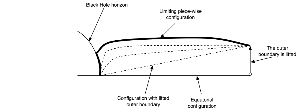
Figure 2: When the outer boundary is slightly lifted the initial configuration relaxed to the one with the least action which is the piece-wise limiting configuration drawn above.

Let us now examine the change rate of the energy of the static configurations coming from the variation of the locations of the inner and outer boundaries. First we consider the inner boundary. If we take into account the piece lying on the horizon, we can say that the inner boundary is always fixed at the initial location. Therefore its contribution should trivially vanish. As mentioned above, we can consider the sequence of static solutions instead of the piece-wise limiting configurations. In this case the inner boundary is varied according to the change of the outer boundary. However, when the inner boundary is on the horizon, we have $\delta r_{0}=0$ and $f_{0}=0$, where the subscript $0$ denotes the value calculated at $\lambda=0$. When the inner boundary is on the axis, $\delta\theta=0$ and $dr/d\theta=0$. Therefore according to the above expression (II) the contribution to the difference in energy from the inner boundary vanishes: $\delta E_{0}=0$.

More complicated is the evaluation of the contribution coming from the outer boundary, $\delta E_{1}$. The total energy is divergent if we consider an infinitely extended object. As a regularization scheme, we cut the configurations at a finite radius. It is convenient to introduce cylindrical coordinates

$$R=r\sin\theta,\qquad Z=r\cos\theta~{}.$$ (6)

For later use, we record the expression of $d\theta/dr$ in terms of $dZ/dR$:

$${d\theta\over dr}={1-\tan\theta{dZ\over dR}\over r\left({dZ\over dR}+\tan\theta\right)}~{}.$$ (7)

We consider the situation in which the outer boundary is varied with $R$ fixed. Since $R$ represents the circumferential radius, fixing $R$ provides a natural way to choose the boundary in a coordinate invariant manner. One could imagine an alternative cutoff radius by fixing the value of $f^{\nu}R$ with an arbitrary power $\nu$. Here we discuss only the simplest case with $\nu=0$, but it is easy to check that any choice of the cutoff radius of this kind leads to the same conclusions. In this sense, the results obtained below are robust. In Appendix we give a little more rigorous justification of this chosen prescription for a regularization scheme.

Since the value of $R$ is fixed at the outer boundary, $\delta r_{1}$ and $\delta\theta_{1}$ are related to each other by the relation

$$\delta R_{1}=\sin\theta_{1}\delta r_{1}+r_{1}\cos\theta_{1}\delta\theta_{1}=0,$$ (8)

where the subscript $1$ denotes the value at $\lambda=1$. The variation of the energy, $\delta E_{1}$, due to displacement of the outer boundary can be written as

$$\delta E_{1}=\left[{\tilde{\sigma}(r\sin\theta)^{p-1}\cos\theta\over\sqrt{1+r^{2}f\left({d\theta\over dr}\right)^{2}}}\left(1-{rf\tan\theta}{d\theta\over dr}\right)\right]_{1}\delta Z_{1}~{}.$$

In the following, we assume that $Z$ becomes almost constant at a large $R$. This is expected because the spacetime is asymptotically Minkowski. This assumption can be directly verified by numerical integration of the equation of motion, and it is visually clear already from Fig. 1. Under this assumption, we have $dZ/dR\ll 1$ and $\tan\theta=R/Z\gg 1$. Thus we find that the first term in parentheses in the denominator of the R.H.S. of Eq. (7) can be safely neglected. At a large distance we can make use of the Newtonian approximation. Namely, we can treat $\delta f$ as a small perturbation denoting $f$ by $1+\delta f$. Using these approximations, we have

$$\delta E_{1}\approx\tilde{\sigma}\left[R^{-q}Z+R^{p-1}{dZ\over dR}\right]_{1}\delta Z_{1},$$ (9)

where $q=d-(p+1)$ represents the co-dimension of the brane. For any type of brane the first term vanishes in the limit $R_{1}\to\infty$. Hence we have

$$\delta E_{1}\mathop{\longrightarrow}_{R_{1}\to\infty}\tilde{\sigma}R_{1}^{p-1}\left({dZ\over dR}\right)_{1}\delta Z_{1}.$$ (10)

If we assume that $\delta E_{1}/\delta Z_{1}$ becomes a constant independent of $R_{1}$ at a large distance, we obtain $dZ/dR\to\tilde{\sigma}{}^{-1}R^{1-p}(\delta E_{1}/\delta Z_{1})$. Then we have the asymptotic behaviour of $Z$ as

$$Z=Z_{\infty}-{R^{2-p}\over(p-2)\tilde{\sigma}}{\delta E_{1}\over\delta Z_{1}},$$ (11)

for $p\geq 3$. $Z_{\infty}$ is the asymptotic value of $Z$. In the case with $p=2$, $Z$ continues to change logarithmically even at a large radius. Here we concentrate on the cases with $p\geq 3$.

It is easy to see from numerical calculations and also it is possible to check analytically that the asymptotic form of the solution is indeed the one mentioned above. In fact, if we write down the equation of motion keeping the terms linear in $Z$ up to $O(\delta f)$, we obtain

$${d^{2}Z\over dR^{2}}+{p-1\over R}{dZ\over dR}=(q-1){Z\over R^{d-1}},$$ (12)

where we neglected the terms of $O(\delta f)$ multiplied by the derivative of $Z$ because $Z$ is almost constant. The right hand side gives the leading order correction due to $\delta f$. we can easily solve the above equation completely neglecting the right hand side as $Z=Z_{\infty}+\alpha R^{2-p}$, where $Z_{\infty}$ and $\alpha$ are integration constants. This solution is completely consistent with the expression (11). We can iteratively evaluate the effect due to the right hand side of Eq.(12). Substituting $Z=Z_{\infty}$ on the right hand side, the correction to $Z$ is obtained as ${q-1\over q(d-3)}Z_{\infty}R^{2-p-q}$. Therefore this correction becomes sub-dominant compared with the term $\alpha R^{2-p}$ for a sufficiently large $R$. Hence, the use of expression (11) is justified.

III Energy of Minkowski-type brane at a large distance

We now consider the energy of static Minkowski-type brane solutions. As we mentioned in the preceding section, we can use Newtonian approximation at large $r$. In other words we expand the solution $Z(R)$ in terms of $\delta f$ as

$$Z(R)=Z_{(0)}+Z_{(1)}+\cdots~{}.$$

The lowest order solution is the one in Minkowski spacetime and it is therefore given by $Z_{(0)}=$ constant. $Z_{(1)}$ is the correction of $O(\delta f)$. The expression for the energy $E$ can be also expanded with respect to $\delta f$ formally as

$$E=E_{(0)}+E_{(1)}+\cdots~{},$$

where

$$E_{(0)} = \tilde{\sigma}\int_{0}^{1}d\lambda\,(r\sin\theta)^{p-1}\sqrt{\left({dr\over d\lambda}\right)^{2}+r^{2}\left({d\theta\over d\lambda}\right)^{2}}~{},$$

$$E_{(1)} = {\tilde{\sigma}\over 2}\int_{0}^{1}d\lambda\,(r\sin\theta)^{p-1}{r^{2}{d\theta\over d\lambda}\over\sqrt{\left({dr\over d\lambda}\right)^{2}+r^{2}\left({d\theta\over d\lambda}\right)^{2}}}\delta f.$$

Then, we have

$$E[Z]=E_{(0)}[Z_{(0)}]+\left(\int d\lambda\,{\delta E_{(0)}\over\delta Z}Z_{(1)}\right)+E_{(1)}[Z_{(0)}]~{},$$

where we have neglected terms of $O\left((\delta f)^{2}\right)$. Since the second term vanishes because $Z_{(0)}=$ constant satisfies $\delta E_{(0)}/\delta Z=0$, we only need to evaluate $E_{(1)}[Z_{(0)}]$ as the lowest order correction of $O(\delta f)$. Substituting $\delta f=-1/r^{d-3}$ and $r\cos\theta=Z_{(0)}$, we have

$$E_{(1)}[Z_{(0)}] = -\tilde{\sigma}Z_{(0)}^{2-q}\int d\theta(\cos\theta)^{q-1}(\sin\theta)^{p-1}$$ (13)

$$\mathop{\longrightarrow}_{R_{1}\to\infty}-\tilde{\sigma}Z_{(0)}^{2-q}{\Gamma\left[p/2\right]\Gamma\left[q/2\right]\over 4\Gamma\left[(p+q)/2\right]}.$$

For any number of co-dimensions $q\geq 1$, the $\theta$-integral converges in the limit $R_{1}\to\infty$. The behaviour of $E_{(1)}[Z_{(0)}]$ is peculiar for the cases with $q=1$ and $q=2$. In the case with $q=1$, $E_{(1)}[Z_{(0)}]$ continues to increase for an increasing value of $Z_{(0)}$. In the case with $q=2$, $E_{(1)}[Z_{(0)}]$ converges to a constant value $\tilde{\sigma}/2p$. In other cases, $E_{(1)}[Z_{(0)}]$ vanishes in the limit $Z_{(0)}\to\infty$.

We can now compare the energy of this asymptotic configuration with the one on the equatorial plane. The difference $E_{(0)}[Z_{(0)}]-E_{\rm equatorial}$ is given by the area of the brane cut by the black hole horizon, $\tilde{\sigma}/p$. Hence, neglecting the terms of $O((\delta f)^{2})$, we have

$$\Delta E\approx\left\{\begin{array}[]{ll}\displaystyle-\tilde{\sigma}Z_{\infty}{\sqrt{\pi}\Gamma[p/2]\over 4\Gamma[(p+1)/2]}&\mbox{for}~{}q=1~{},\cr\displaystyle{\tilde{\sigma}\over 2p}&\mbox{for}~{}q=2~{},\cr\displaystyle{\tilde{\sigma}\over p}&\mbox{for}~{}q\geq 3~{},\end{array}\right.$$ (17)

for a large value of $Z_{\infty}$, where we have defined

$$\Delta E\equiv E[Z_{\infty}]-E_{\rm equatorial}~{}.$$ (18)

A way of interpreting the previous results is to write down the equation for the gravitational field:

$$\Box h_{\mu\nu}=T_{\mu\nu}-{1\over d-2}g_{\mu\nu}T~{},$$

where $T_{\mu\nu}$ is the stress tensor coming from the brane. By taking the $00$ component we obtain an equation for the gravitational potential $h_{00}$:

$$\Box h_{00}={q-2\over 2(d-2)}T_{00}~{}.$$

The coefficient in the previous expression describes what happens: for $q=1$ the sign is negative and the potential is repulsive, for $q>2$ the sign is positive and the potential is attractive. The case of $q=2$ is marginal.

These results are completely in harmony with those obtained in the opposite approximation in which the black hole is treated as a test particle on the background spacetime determined by the gravity of the brane. In this approximation, co-dimension one branes cannot be embedded in an asymptotically flat spacetime. The simplest solution with the highest symmetry is the Vilenkin-Ipser-Sikivie model. We prepare two copies of Minkowski spacetime and consider the inside of the hyperboloid whose invariant distance from the origin is constant. Placing a brane on this hyperboloid means gluing together two copies of Minkowski spacetime there. Since the bulk is simply given by Minkowski spacetime in this model, the trajectory of a test particle is just a straight line. On the other hand, the brane moves along a hyperboloid, and hence the brane is always accelerated outward. To the contrary, if we look at a test particle moving in the bulk from the brane, it is accelerated in the direction leaving from the brane. Namely, the force acting on the particle looks repulsive.

When we consider a co-dimension two brane, we can recall a cosmic string in four dimensional spacetime, which we know is described by Minkowski spacetime with a deficit angle. For co-dimension two branes in general dimensions, the same is true. Therefore a particle moving far from the brane does not feel the gravity force due to the brane at all. This is consistent with the fact that the derivative of the energy $dE_{(1)}[Z_{(0)}]/dZ_{(0)}$ computed from Eq. (13) vanishes for $q=2$. For higher co-dimensions, gravity force caused by a brane is attractive and is proportional to $\ell^{1-q}$, where $\ell$ is the distance between the brane and the particle. This dependence on $\ell$ also agrees with the estimate from the derivative of the energy (13).

IV potential barrier for the escape of black hole

In the present section we will complement the analytical results of the preceding section by numerical estimates. To start with, we can compute the profile of the potential along the path of escape of Fig. 1 by calculating the difference of the regularized energy for the sequence of static solutions numerically. Here, due to technical simplicity, instead of evaluating the energies of the solutions directly, we evaluate at finite radius the difference in energy for neighboring configurations by using formula (9). Fig. 3 shows the plots of $\{Z_{\infty},\kappa\}$ with

$$\kappa\equiv{1\over\tilde{\sigma}}{\delta E~{}\over\delta Z_{\infty}}~{},$$ (19)

for various co-dimensions.

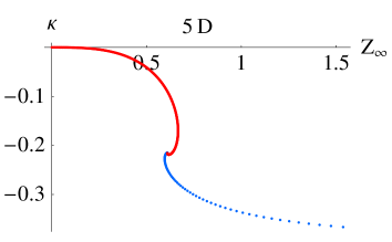
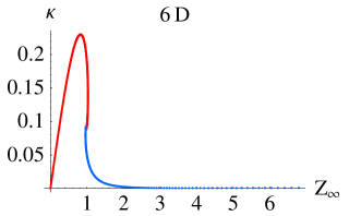
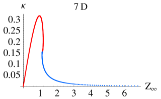
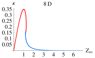
Figure 3: The figure shows the plots of $\{Z_{\infty},\kappa\}$ for a $p=3$ brane in a $d=5,6,7,8$ dimensional bulk respectively. The red line corresponds to the brane intersecting the black hole, whereas the blue line corresponds to the brane outside the black hole.

The close-up views of Fig. 4 illustrate the transition point where the brane pinches and goes from a configuration intersecting the black hole to the detached one with Minkowski topology.

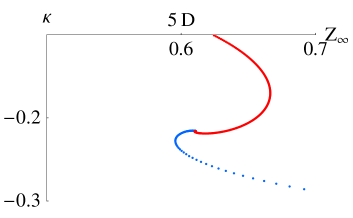
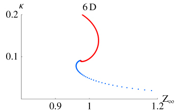
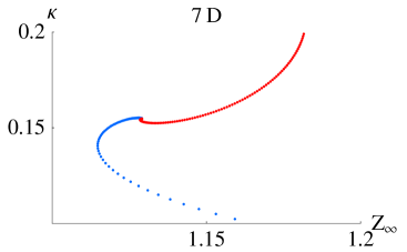
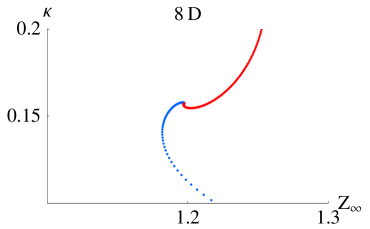
Figure 4: Transition between black hole topology to Minkowski topology.

Finally, in Fig. 5 we plot the value of the energy $\Delta E$ vs $Z_{\infty}$. Here $\Delta E$, defined by Eq. (18), is evaluated by the integral $\Delta E=\int dZ_{\infty}(\delta E/\delta Z_{\infty})$. The asymptotic values of $\Delta E$ in the limit $Z_{\infty}\to\infty$ are consistent with the analytic estimates given in Eq. (17).

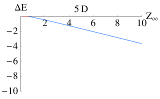
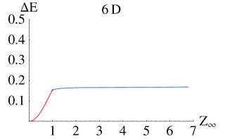
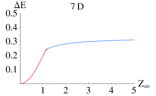
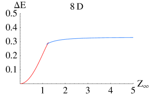
Figure 5: The figure shows the dependence of $\Delta E$ on $Z_{\infty}$ for $d=5,6,7,8$ and $p=3$.

Fig. 6 illustrates the detailed structure of the profile for the energy in the region near the pinching. Besides this tiny structure the curves are monotonically decreasing for co-dimension one branes and increasing for the other cases. The most important point is that there is no energy barrier which is higher than the initial value for co-dimension one branes. For the other cases with higher co-dimensions, the barrier height does not exceed the asymptotic value at $Z_{\infty}\to\infty$. These features can be more easily shown by considering the energy of a momentarily static configuration with $Z=$constant. The energy for this configuration is given by

$$E_{Z=\rm const.}=\tilde{\sigma}\int dRR^{p-1}\sqrt{1-Z^{2}(R^{2}+Z^{2})^{-(d-1)/2}}.$$

The plots of this simple expression are similar to but slightly bigger than the results shown in Fig. 5. This simple expression gives an upper bound on the potential obtained by correctly solving the equation of motion for static configurations. Therefore this simplified potential is sufficient to show that there is no significantly high bump in the profile of the potential.

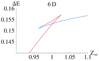
Figure 6: Close up of the profile in the region near pinching. The red branch represents the brane configurations attached to the black hole; the blue branch represents the brane separated from the black hole. The plot refers to the case $d=6$, $p=3$.

In Fig. 6 we can distinguish three branches describing the evolution of the brane: the (stable) black hole branch where the brane intersects the black hole horizon, the (stable) Minkowski branch where the brane lies outside the black hole horizon and finally an unstable branch joining the first two. This last unstable branch contains the configuration attached to the pole at $\theta=0$ on the event horizon, which we call the pinching configuration. This configuration represents a kind of ‘geometric threshold’ between the configurations that intersect the black hole and those that do not. If we closely look at the vicinity of the pinching configuration, there is a finer structure art1 , which is beyond the resolution of the plot given in Fig. 6. Schematically, these three branches are drawn in Fig. 7.

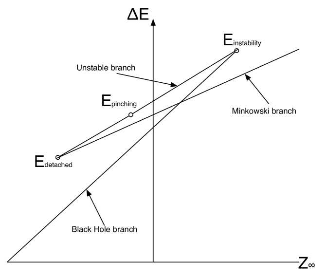
Figure 7: Schematic representation of Fig. 6.

Accordingly, we can distinguish three energy scales: $E_{pinching}$, $E_{detached}$ and $E_{instability}$. $E_{pinching}$ labels the energy of the pinching configuration. The values of $E_{pinching}$ are tabulated in Table 1 for all dimensions and co-dimensions up to $d=11$.

$p\diagdown d$	$6$	$7$	$8$	$9$	$10$	$11$
3	0.1523	0.2405	0.2830	0.3044	0.3158	0.3223
4	-	0.1171	0.1800	0.2099	0.2254	0.2340
5	-	-	0.0962	0.1477	0.1706	0.1822
6	-	-	-	0.0820	0.1251	0.1436
7	-	-	-	-	0.0687	0.1081
8	-	-	-	-	-	0.0608

Table 1: Values of $E_{pinching}$ for $d=6,...,11$ and $p=3,...,8$.

$E_{detached}$ represents the minimum energy of a configuration detached from the black hole. It is interesting to note that such ‘detached’ configuration cannot be reached through a sequence of static solutions starting from the initial equatorial configuration, but nevertheless it marks the threshold for the separation between the brane of the black hole, which can in principle be reached via some different (dynamical) deformation of the brane. Finally, $E_{instability}$ represents the value of the energy corresponding to the upper cusp (see Fig. 7), which marks an onset of instability. If the brane starts from the initial equatorial configuration and goes through the sequence of static solution it will reach such ‘instability’ point. The question is what happens when this instability point is passed over. If we introduce dissipation we can expect that the brane will evolve towards a configuration with lower energy lying on the Minkowski branch and therefore a configuration separated from the black hole will be realized. As one can notice from Fig. 5, the difference between the values of $E_{pinching}$, $E_{detached}$ and $E_{instability}$ is very small. Some values of $E_{detached}$ and $E_{instability}$ are tabulated in Table 2 for $p=3$ and $d=6,...,11$.

$d$	$6$	$7$	$8$	$9$	$10$	$11$
$E_{instability}$	0.1574	0.2491	0.2926	0.3145	0.3264	0.3333
$E_{detached}$	0.1510	0.2384	0.2806	0.3019	0.3134	0.3200

Table 2: $E_{instability}$ and $E_{detached}$ for $p=3$ and $d=6,...,11$

As anticipated, we find that the co-dimension one brane is peculiar in the sense that it does not have a barrier for the escape of black hole. This means that there is no critical escape velocity in the present approximation where the brane tension is not very large. By contrast, all other types of branes have a barrier. Roughly speaking, the height of the energy barrier is $O(\sigma(G_{d}m)^{p/(d-3)})$ where we have explicitly written the $d-$dimensional Newton constant $G_{d}$ and the black hole mass $m$. Then, by equating the kinetic energy of the black hole $mv^{2}/2$ with this energy barrier, the critical escape velocity $v_{c}$ will be estimated as $v_{c}\approx\sqrt{\sigma G_{d}^{p/(d-3)}m^{(2-q)/(d-3)}}$. Very interestingly, the critical escape velocity $v_{c}$ is independent of the mass of the black hole for co-dimension two branes ($q=2$). In the cases with higher co-dimensions $v_{c}$ is smaller for a black hole with a larger mass, as is expected from the larger inertia of the black hole.

V discussion

In this paper we investigated a system composed of a brane and a black hole when a perturbation gives the black hole a relative velocity with respect to the brane. The principal problem we are interested in is the phenomena of escape of the black hole. The main goal of our study is to clarify whether the effect of the brane tension may prevent the black hole from escaping for small recoil velocities and to understand whether a critical escape velocity exists.

Here, we analyzed this problem by studying the interaction between a Dirac-Nambu-Goto brane and a black hole assuming adiabatic (quasi-static) evolution. By ‘quasi-static’ we mean that the system evolves very slowly going through configurations which are stationary. Taking the brane lying on the equatorial plane of the black hole as initial configuration, we considered the brane in a fixed Schwarzschild spacetime background, neglecting the gravitational perturbation caused by the brane, approximation which is adequate in the case of small tension. Our strategy is to compute the energy for the sequence of the static solutions describing the escape as shown in Fig. 1 directly and see how the energy changes along the easiest path for the black hole to escape. From this knowledge we can estimate in which cases there is a potential barrier that prevents the separation and the initial energy necessary to overcome such a barrier.

We gave an analytic estimate for the height of the potential by comparing the energies of the initial and the final configurations, where ‘final configuration’ refers to the one with the black hole disconnected and being far away from the brane. We also computed the energy of each static configuration numerically, thus providing support to the analytical estimates. From the calculated shape of the potential, we find that there is no barrier in the potential for co-dimension one branes, meaning that the configuration with a black hole attached to a co-dimension one brane is unstable. In contrast, when the co-dimension of the brane is equal to or greater than two, there is a potential barrier along the escape path of the black hole, and the critical escape velocity is evaluated to be $O(\sqrt{\sigma G_{d}^{(d-q-1))/(d-3)}m^{(2-q)/(d-3)}})$, where $d$ and $q$ are the spacetime dimension and brane co-dimension, respectively.

In Ref. art3 , we studied the phenomena of escape treating the brane as a domain wall in a scalar effective field theory. Since here we have focused on the case Dirac-Nambu-Goto branes, it is interesting to ask whether the results of this paper are also valid when the brane has a thickness. We expect that even in the case of thick branes described by field theoretical topological defects, the analytic comparison of the energies between the initial and the final state will not change dramatically. For the final configuration the description by a Dirac-Nambu-Goto brane is always a good approximation. For the initial configuration, the contribution to the energy from the region near the horizon may be corrected, especially when the thickness of the defect is not very small compared with the horizon radius. However, the height of the barrier in the intermediate stage is potentially quite different, and therefore a more rigorous study of the thick case is necessary to make a definite statement.

As we mentioned in the introduction, one of the main motivations that led us to consider the problem of how a black hole interacts with a domain wall is related to the possibility of observing mini black holes in collider experiments or in cosmic rays. In this context Ref. stoj points out that the escape of the black hole might provide a way of distinguishing between various models. Specifically, one possible difference might come out from the fact that, contrary to models with large extra dimensions r1 ; r1-1 , warped models have additional $Z_{2}-$symmetry r2 , which makes the brane behave as if the tension were infinite, resulting in the impossibility for mini black holes to leave the brane. This is, however, not the case in models when the $Z_{2}-$symmetry is relaxed, as Refs. art1 ; art2 ; art3 have shown. The results presented here take a further step in this direction and suggest that also within models of the same class, without $Z_{2}-$symmetry, the co-dimensionality has a remarkable effect. If the co-dimension is $1$, then even for small recoil velocity the black hole is expected to slide off the brane, contrary to the higher co-dimension case where there is an energy barrier that would prevent this from occurring.

At this point it seems interesting to compare the recoil velocity due to Hawking radiation to the critical velocity. If we assume that the recoil is due to inhomogeneous Hawking emission, a rough estimate gives $v_{rec}\simeq 1/\sqrt{N}$, where $N\simeq m/T_{H}$ is the number of emitted particles and $T_{H}\approx r_{H}^{-1}$ is the Hawking temperature. The horizon radius $r_{H}$ is given by $(m/M_{d}^{d-2})^{1\over d-3}$ with $M_{d}$ being the higher dimensional Planck scale. Thus, we have

$$v_{rec}/v_{cr}\simeq\left({M_{d}\over m}\right)^{1+p\over 2d-6}\left({M_{d}^{1+p}\over\sigma}\right)^{1/2}~{},$$ (20)

From this equation, we can compute the critical value for the mass at which the recoil velocity equals the critical velocity:

$$m_{cr}\simeq{M_{d}^{d-2}\over\sigma^{d-3\over p+1}}~{}.$$

Thus we can say that, if the initial black hole mass is smaller than the critical mass, the recoil velocity is expected to exceed the critical one before long, and therefore the black hole will leave the brane during the early stage of its evaporation. On the other hand, if the mass of the black hole is larger than $m_{cr}$, we expect that the black hole will escape from the brane in a subsequent stage after its mass becomes as small as $m_{cr}$ after losing a significant portion of its initial mass.

Finally we want to mention the validity range of the probe-brane approximation. The probe-brane approximation will require that the mass of the portion of the brane near the black hole horizon is much smaller than the black hole mass:

$$\sigma r_{H}^{p}\ll m\,.$$

This gives a constraint

$$m\gg M_{d}\left({\sigma\over M_{d}^{p+1}}\right)^{{d-3\over q-2}}~{}.$$

This constraint is not so stringent. As far as the brane tension is small in the higher dimensional Planck units, our approximation will be kept to be valid throughout the above-mentioned process of black hole evaporation until its escape from the brane at $m\approx m_{cr}$.

Appendix A justification of the regularization procedure

We present one argument for justification of using the cutoff at a fixed circumferential radius. One way to make the energy well defined is to fix the outer boundary configuration completely; not only the position of the brane but also the gravitational field. More precisely, for example, fixing the boundary induced metric will be appropriate. This is impossible in the present setup since the spacetime is exactly given by Schwarzschild spacetime. If we fix the location of the brane at the boundary, a different static solution corresponds to a different position of the black hole. Then, the induced metric on the boundary changes. To fix the boundary metric, we need to include metric perturbations.

For clarity, we can consider the Newtonian picture. We set the outer boundary at $r=r_{o}$ and the brane is on the equatorial plane on the boundary. Then, the perturbation of the Newtonian potential $\phi$ necessary to compensate the change of the location of the central black hole will be evaluated as

$$\delta\phi\approx{d-3\over 2}{Z\over r_{o}^{d-1}}\delta Z.$$ (21)

Here $G_{d}m$ is set to unity as before. The leading order perturbation of the gravitational potential will be given by a dipole field $\delta\phi={d-3\over 2}{Z\delta Z\over r_{o}^{d-1}}$, which scales as $\sim 1/r_{o}^{d-1}$ for large $r_{o}$. The total amount of correction due to this perturbation of the gravitational potential to the gravitational binding energy of the brane will scale like $\delta\phi$ multiplied by the area of the brane $\sim r_{o}^{p}$. Hence it scales as $\sim 1/r_{o}^{q}$. We can therefore neglect this contribution in the limit $r_{o}\to\infty$. The correction to the energy due to gravitational perturbations is quadratic in $\delta\phi$. Hence, its contribution scales as $\delta\phi^{2}\times r^{d-1}\propto 1/r_{o}^{d-1}$, and we can neglect it safely. When we take into account the gravity, we also need to consider gravitational potential induced by the brane. However, the background gravitational potential is chosen to be a vacuum solution. Then the leading order correction is quadratic. Therefore it scales like $\sigma^{2}$. In the end, we claim that the effect of gravity can be completely neglected when the outer boundary radius $r_{o}$ is moved to infinity as far as we consider energy of $O(\sigma)$.

References

- (1) N. Arkani-Hamed, S. Dimopoulos and G. R. Dvali, Phys. Lett. B 429, 263 (1998).
- (2) I. Antoniadis, N. Arkani-Hamed, S. Dimopoulos and G. R. Dvali, Phys. Lett. B 436, 257 (1998).
- (3) P.C. Argyres, S. Dimopoulos, J. March-Russell, Phys. Lett. B 441, 96 (1998).
- (4) L. Randall and R. Sundrum, Phys. Rev. Lett. 83, 3370 (1999).
- (5) S. Dimopoulos and G. Landsberg, Phys. Rev. Lett. 87 (2001) 161602.
- (6) S. B. Giddings and S. Thomas, Phys. Rev. D65 (2002) 056010.
- (7) J.L. Feng, A.D. Shapere, Phys. Rev. Lett. 88 (2002) 021303.
- (8) R. Emparan, G.T. Horowitz, and R.C. Myers, Phys. Rev. Lett. 85 (2000) 499.
- (9) V. P. Frolov, D. Stojkovic, Phys. Rev. Lett. 89 (2002) 151302; Phys. Rev. D67 (2003) 084004.
- (10) A. Flachi, T. Tanaka, Phys. Rev. Lett. 95 161302 (2005).
- (11) M. Christensen, V. P. Frolov, A.L. Larsen, Phys. Rev. D58 (1998) 085008; Phys. Rev. D59 (1999) 125008.
- (12) A. Flachi, O. Pujolàs, M. Sasaki and T. Tanaka, [hep-th/0601174]
- (13) D. Stojkovic, Phys. Rev. Lett. 94 (2005) 011603.
- (14) F. R. Tangherlini, Nuovo Cim. B 77, (1963) 636.
- (15) R. C. Myers and M. J. Perry, Annals Phys. 172 (1986) 304.