Topological structure of the vortex solution in Jackiw-Pi model

Abstract

By using $\phi$ -mapping method, we discuss the topological structure of the self-duality solution in Jackiw-Pi model in terms of gauge potential decomposition. We set up relationship between Chern-Simons vortex solution and topological number which is determined by Hopf index and Brouwer degree. We also give the quantization of flux in this case. Then, we study the angular momentum of the vortex, it can be expressed in terms of the flux.

I introduction

Chern-Simons theories exhibit many interesting and important properties. They are based on secondary characteristic classes discovered in Ref.cs01 and many topological invariants of knots and links discovered in the 1980s could be reinterpreted as correlation functions of Wilson loop operators in Chern-Simons theorywt03 . Moreover, for gauge theories and gravity in three-dimensions, they can appears as natural mass terms and will lead to a quantized coupling constant as well as a mass after quantizationdj02 . They have also found applications to a lot of physical problems, such as particle physics, quantum Hall effect, quantum gravity and string theoryykf ; ba98 ; jp01 ; re01 ; qh01 ; re02 ; re03 ; re04 ; re05 ; wt01 ; wt02 . Chern-Simons term acquire dynamics via coupling to other fieldsah01 ; ba98 , and get multifarious gauge theory, all of which have vortex solutions, these static solutions can be obtained when their Hamiltonian was minimal. Vortices and their dynamics are interesting objects to be studiedah01 ; pd02 ; pd23 ; pd33 ; pd43 . R. Jackiw and S-Y. Pi considered a gauged, nonliner Schödinger equation in two spatial dimensions, with describes nonrelativistic matter interacting with Chern-Simons gauge fields. Then they find explicit static, self-dual solutions which satisfies the Liouville equation.

In this paper, we will discuss topological structure of the self-duality solution in Jackiw-Pi model in terms of gauge potential decompositiondg01 ; du01 ; sa01 ; li04 ; li05 . We will look for complete vortex solution from self-duality equation and set up the relationship between the vortex solution and topological number. We also study the quantization of the flux of the vortex. Last, we will investigate the angular momentum of the vortex.

II Self-duality solutions in Jackiw-Pi Model

In this section, making use of the self-duality equation, we will look for complete vortex solution in Jackiw-Pi modelba98 by using the decomposition of gauge potential. The Abelian Jackiw-Pi model in nonlinear Schrödinger systems is

$$\pounds_{jp}=\frac{\kappa}{2}\epsilon^{\mu\nu\lambda}A_{\mu}\partial_{\nu}A_{\lambda}+i\hbar\Psi^{*}D_{0}\Psi-\frac{\hbar^{2}}{2m}|\mathbf{D}\Psi|^{2}+\frac{g}{2}(\Psi^{*}\Psi)^{2}.$$ (1)

[We use relativistic notation with the metric diag(1,-1,-1) and $x^{\mu}=(ct,\mathbf{r})$.] Where $\mathbf{D}=\mathbf{\nabla}-i\frac{e}{\hbar c}\mathbf{A}$ and $\Psi$ is ”matter” field, the first term is the Chern-Simons density, which is not gauge invariant. Also $m$ is the mass parameter, $A_{\mu}$ is gauge potentials, $g$ governs the strength of nonlinearity, $\kappa$ controls the Chern-Simons addition and provides a cutoff at large distance greater than $\frac{1}{\kappa}$ for gauge-invariant electric and magnetic fields, which can be written as $\mathbf{E}=-\nabla\mathbf{A}^{0}-(\frac{1}{c})\partial_{t}\mathbf{A}$, and $\mathbf{B}=\mathbf{\nabla}\times\mathbf{A}$. Thus the Chern-Simons terms gives rise to massive, yet gauge-invariant ”electrodynamics”. The last term represents a self-coupling contact term of the type commonly found in nonlinear Schr odinger systems. The Euler-Lagrange equations are

$$iD_{0}\Psi=-\frac{1}{2m}\mathbf{D}^{2}\Psi-g\left|\Psi\right|^{2}\Psi,F_{\mu\nu}=\frac{1}{\kappa}\varepsilon_{\mu\nu\rho}J^{\rho}.$$ (2)

The energy density is

$$\mathcal{H}=\frac{\hbar^{2}}{2m}|\mathbf{D}\Psi|^{2}-\frac{g}{2}(\Psi^{*}\Psi)^{2},$$ (3)

in which $g=\mp\frac{e^{2}\hbar}{mck}$, by

$$|\mathbf{D}\Psi|^{2}=|(D_{1}\pm iD_{2})\Psi|^{2}\pm\frac{m}{\hbar}\mathbf{\nabla}\times\mathbf{J}\pm\frac{e}{\hbar c}B\Psi^{*}\Psi,$$ (4)

and

$$B=\epsilon^{ij}\partial_{i}A^{j}=-\frac{e}{k}\rho,$$ (5)

we can get

$$\mathcal{H}=\frac{\hbar^{2}}{2m}|(D_{1}\pm iD_{2})\Psi|^{2}\pm\frac{\hbar}{2}\nabla\times\mathbf{J}-\left[\frac{g}{2}\pm\frac{e^{2}\hbar}{2mck}\right](\Psi^{*}\Psi)^{2}.$$ (6)

where $e$ measure the coupling to gauge field described by scalar $A^{0}$ and vector $\mathbf{A}$ potentials. With $g=\mp\frac{e^{2}\hbar}{mck}$, and sufficiently well-behaved fields so that the integral over all space of $\nabla\times\mathbf{J}$ vanishes, the energy is

$$H=\int d\mathbf{r}\mathcal{H}=\frac{\hbar^{2}}{2m}\int d\mathbf{r}|(D_{1}\pm iD_{2})\Psi|^{2}.$$ (7)

This is non-negative and vanishes. Thus attaining its minimum when $\Psi$ satisfies a self-dual equation

$$D_{1}\Psi=\mp iD_{2}\Psi.$$ (8)

To solve Eq.(8),we note that when $\Psi$ is decomposed into two scalar fields

$$\Psi=\Psi_{1}+i\Psi_{2},$$ (9)

We can define a unit vector field $\mathbf{n}$ as follows

$$n^{a}=\frac{\Psi_{a}}{(\Psi^{*}\Psi)^{\frac{1}{2}}},a=1,2.$$ (10)

It is easy to prove that $\mathbf{n}$ satisfies the constraint conditions

$$n^{a}n^{a}=1,n^{a}dn^{a}=0.$$ (11)

From Eq.(8), and making use of the decomposition of U(1) gauge potential in terms of the two-dimensional unit vector field $\mathbf{n}$, we can obtain

$$A^{i}=\frac{\hbar c}{e}(\epsilon^{ab}n^{a}\partial_{i}n^{b}\pm\frac{1}{2}\epsilon^{ij}\partial_{j}\ln\rho),$$ (12)

From Eq.(5) and Eq.(12) we get

$$B=\frac{\hbar c}{e}\epsilon^{ij}\epsilon^{ab}\partial_{i}n^{a}\partial_{j}n^{b}\pm\frac{\hbar c}{2e}\nabla^{2}\ln\rho,$$ (13)

i.e.

$$-\frac{e}{k}\rho=\frac{\hbar c}{e}\epsilon^{ij}\epsilon^{ab}\partial_{i}n^{a}\partial_{j}n^{b}\pm\frac{\hbar c}{2e}\nabla^{2}\ln\rho.$$ (14)

This equation can be rewritten as

$$\nabla^{2}\ln\rho=\pm\frac{2e^{2}}{\hbar ck}\rho\pm 2\epsilon^{ij}\epsilon^{ab}\partial_{i}n^{a}\partial_{j}n^{b}.$$ (15)

With the help of the $\phi$ -mapping methoddu01 ; sa01 , Eq.(15) can be written as

$$\nabla^{2}\ln\rho=\pm\frac{2e^{2}}{\hbar ck}\rho\pm 4\pi\delta^{2}(\mathbf{\Psi})J\left(\frac{\mathbf{\Psi}}{\mathbf{x}}\right),$$ (16)

in which $J\left(\frac{\mathbf{\Psi}}{\mathbf{x}}\right)$ is Jacobian and

$$J\left(\frac{\mathbf{\Psi}}{\mathbf{x}}\right)=\frac{1}{2}\epsilon^{ab}\epsilon^{ij}\frac{\partial\Psi_{a}}{\partial x^{i}}\frac{\partial\Psi_{b}}{\partial x^{j}},i,j=1,2.$$ (17)

When $\rho\neq 0$, Eq.(16) will be the Liouville equation,

$$\nabla^{2}\ln\rho=\pm\frac{2e^{2}}{\hbar ck}\rho,$$ (18)

as we all know, the Eq.(18) has the general real solution as follows

$$\rho=\kappa\nabla^{2}\ln\left(1+|f|^{2}\right),$$ (19)

where $f=f(z)$ is a holomorphic function of $z=x^{1}+ix^{2}$ only.

Using $f(z)=(\frac{z_{0}}{z})^{N}$, it is easy to obtain the radially symmetric solutions with $r\neq 0$ ax01

$$\rho=\pm\frac{4N^{2}}{r_{0}^{2}}\frac{\hbar c\kappa}{e^{2}}\frac{\left(\frac{r}{r_{0}}\right)^{2(N-1)}}{\left(1+\left(\frac{r}{r_{0}}\right)^{2N}\right)^{2}}.$$ (20)

Because $\rho$ is the charge density of the vortex, it must be positive, the Liouville equation is

$$\nabla^{2}\ln\rho=-\frac{2e^{2}}{\hbar c|\kappa|}\rho,$$ (21)

so the Eq.(20) should be

$$\rho=\frac{\hbar c}{e^{2}}\frac{4|\kappa|N^{2}}{r_{0}^{2}}\frac{\left(\frac{r}{r_{0}}\right)^{2(N-1)}}{\left(1+\left(\frac{r}{r_{0}}\right)^{2N}\right)^{2}},$$ (22)

and the Eq.(16) can be rewritten as

$$\nabla^{2}\ln\rho=-\frac{2e^{2}}{\hbar c|\kappa|}\rho-\frac{\kappa}{|\kappa|}4\pi\delta^{2}(\Psi)J\left(\frac{\mathbf{\Psi}}{\mathbf{x}}\right).$$ (23)

III the topological structure of the vortex solution and its magnetic flux

In this section, making use of Eq.(23), we will discuss the topological structure of the vortex solution, then we will study the magnetic flux of the vortex. Under the radially symmetric, $\nabla^{2}\ln\rho$ can be expressed as

$$\nabla^{2}\ln\rho=\frac{\partial^{2}}{\partial^{2}r}\ln\rho+\frac{1}{r}\partial_{r}\ln\rho.$$ (24)

Substituting Eq.(22) into Eq.(24), we can get

$$\nabla^{2}\ln\rho=-\frac{8N^{2}(\frac{r}{r_{0}})^{2N-2}}{r_{0}^{2}[1+(\frac{r}{r_{0}})^{2N}]^{2}}+2(N-1)\nabla\left(\frac{\mathbf{r}}{r^{2}}\right).$$ (25)

Integrating Eq.(23)

$$\int\nabla^{2}\ln\rho d\mathbf{r}=\int\left[-\frac{2e^{2}}{\hbar c|\kappa|}\rho-\frac{\kappa}{|\kappa|}4\pi\delta^{2}(\mathbf{\Psi})J\left(\frac{\mathbf{\Psi}}{\mathbf{x}}\right)\right]d\mathbf{r}.$$ (26)

Suppose that the vector field $\Psi^{a}$ possess one isolated zeros which is in $x=0$, according to the $\delta$-function theorydelt , $\delta^{2}(\mathbf{\Psi})$ can be expressed by

$$\delta^{2}(\mathbf{\Psi})=\frac{\beta\delta^{2}(\mathbf{x})}{\mid J\left(\frac{\mathbf{\Psi}}{\mathbf{x}}\right)\mid_{\mathbf{x}=0}},$$ (27)

and then one can obtain

$$\int 4\pi\delta^{2}(\mathbf{\Psi})J\left(\frac{\mathbf{\Psi}}{\mathbf{x}}\right)d\mathbf{r}=4\pi\int\beta\eta\delta^{2}(\mathbf{x})d\mathbf{r},$$ (28)

where $\beta$ is positive integer (the Hopf index of the zero point) and $\eta$, the Brouwer degree of the vector field $\mathbf{\Psi}$,

$$\eta=sgnJ\left(\frac{\mathbf{\Psi}}{\mathbf{x}}\right)|_{\mathbf{x=0}}=\pm 1.$$ (29)

The meaning of the Hopf index $\beta$ is that while $\mathbf{x}$ covers the region neighbouring the zero point once, the vector field $\mathbf{\Psi}$ covers the corresponding region $\beta$ times, Hence, $\beta$ and $\eta$ are the topological number which shows the topological properties of the vortex solution. We have

$$\delta^{2}(\mathbf{\Psi})J\left(\frac{\mathbf{\Psi}}{\mathbf{x}}\right)=\beta\eta\delta^{2}(\mathbf{x}).$$ (30)

If we define the topological number $Q$ as

$$Q=\int\delta^{2}(\mathbf{\Psi})J\left(\frac{\mathbf{\Psi}}{\mathbf{x}}\right)d\mathbf{r}=\beta\eta,$$ (31)

from Eq.(26) we can get

$$N-1=-\frac{\kappa}{|\kappa|}Q.$$ (32)

Substituting Eq.(32) into Eq.(22), we can obtain

$$\rho=\frac{\hbar c}{e^{2}}{4|\kappa|(-\frac{\kappa}{|\kappa|}Q+1)^{2}\over r_{0}^{2}}{\left(\frac{r}{r_{0}}\right)^{-2\frac{\kappa}{|\kappa|}Q}\over\left(1+\left(\frac{r}{r_{0}}\right)^{2(-\frac{\kappa}{|\kappa|}Q+1)}\right)^{2}},$$ (33)

It is obviously Eq.(33) is the solution of Eq(23). On the other hand, this means vortex density $\rho$ relates to its topological number $Q$. We now see that $N$ must be an integer.

If we note the unit magnetic flux $\Phi_{0}=\frac{2\pi\hbar c}{e}$, one can get

$$\int_{0}^{\infty}\mathbf{B}d\mathbf{r}=-4\pi\kappa\left|\frac{N}{\kappa}\right|\frac{\hbar c}{e}=-2\frac{\kappa}{|\kappa|}\Phi_{0}\left|-\frac{\kappa}{|\kappa|}Q+1\right|,$$ (34)

from this equation we know the magnetic flux is quantized. When the total topological charge equal to zero, the magnetic flux of this vortex is

$$\Phi=\int_{0}^{\infty}\mathbf{B}d\mathbf{r}=-2\frac{\kappa}{|\kappa|}\Phi_{0}.$$ (35)

See Figure [1] for a plot of the density with the $Q=0$ case, and Figure [2] with the $Q=1$ case. Note the ring-like form of the magnetic field for these Chern-Simons vortices, as the magnetic field is proportional to $\rho$, so $\mathbf{B}$ vanishes where the field $\Psi$ vanishes. We define $r_{v}$ is the radius of the vortex, which satisfies

$$\rho_{max}=\rho(r_{v}),$$ (36)

so $r_{v}$ is the solution of the equation

$$\frac{\partial\rho}{\partial r}=0,$$ (37)

hence

$$r_{v}=r_{0}\left(1-\frac{2}{-\frac{\kappa}{|\kappa|}Q+1}\right)^{\frac{1}{-2\frac{\kappa}{|\kappa|}Q+2}}.$$ (38)

In Figure [1] and Figure [2], the radius of the vortex is $\frac{r_{v}}{r_{0}}$, and the height of the vortex is $\rho_{max}$. Figure [3] shows the values of the radius of the vortex as $Q$ is varied when $\kappa<0$.

The height of the vortex

$$\rho_{max}=\frac{\hbar c|\kappa|}{r_{0}^{2}e^{2}}\left(\frac{\frac{\kappa}{|\kappa|}Q}{\frac{\kappa}{|\kappa|}Q-2}\right)^{\frac{1}{\frac{\kappa}{|\kappa|}Q-1}}\left(\left(\frac{\kappa}{|\kappa|}Q-1\right)^{2}-1\right).$$ (39)

Figure [4] shows the values of the height of the vortex as $Q$ is varied when $\kappa<0$.

IV the angular momentum of the vortex

The density $\mathcal{J}$ for the angular momentum $\mathbf{J}$ isjp01

$$\mathcal{J}=m\mathbf{r}\times\mathbf{j},$$ (40)

in which

$$\mathbf{j}=\mp\frac{\hbar}{2m}\nabla\times\rho,$$ (41)

so we can obtain the angular momentum

$$\mathbf{J}=m\int d\mathbf{r}\left[\mathbf{r}\times\left(\mp\frac{\hbar}{2m}\nabla\times\rho\right)\right]=\pm\frac{2\hbar k}{e}\left(\frac{-\kappa}{|\kappa|}Q+1\right)\Phi_{0}=\pm\frac{\kappa\hbar}{e}\Phi.$$ (42)

where topological number $Q$ must be an integer. This equation shows $J$ is the magnetic dipole moment.

V Conclusions

When added the usual Maxwell action to Chern-Simons, the resulting theory represents a single local degree of freedom, paradoxically endowed with a finite range but still gauge invariant. In this paper, we studied the topological structure of Chern-Simons vortex in Jakiw-Pi model. We also obtain the charge of the vortex which is determined by Hopf index and Brouwer degree. Secondly, compare with Jakiw’s results, we get a Liouville equation with a $\delta$ function, then we also obtain the solution of this equation, and the $\delta$ function will not change the character of the solution when $\rho\neq 0$. Lastly, we calculate the integral of the Liouville equation and find the relationship between topological number and the solution of Liouville equation, we also find that the flux is quantized from the integral value of the solution in the whole space. However, the flux is non-vanish when the topological number equals to zero. So does the the angular momentum.

VI acknowledgments

This work was supported by the CAS Knowledge Innovation Project (No.kjcx2-sw-No2;No.kjcx2-sw-No16) and Science Foundation of China (10435080, 10275123).

VII references

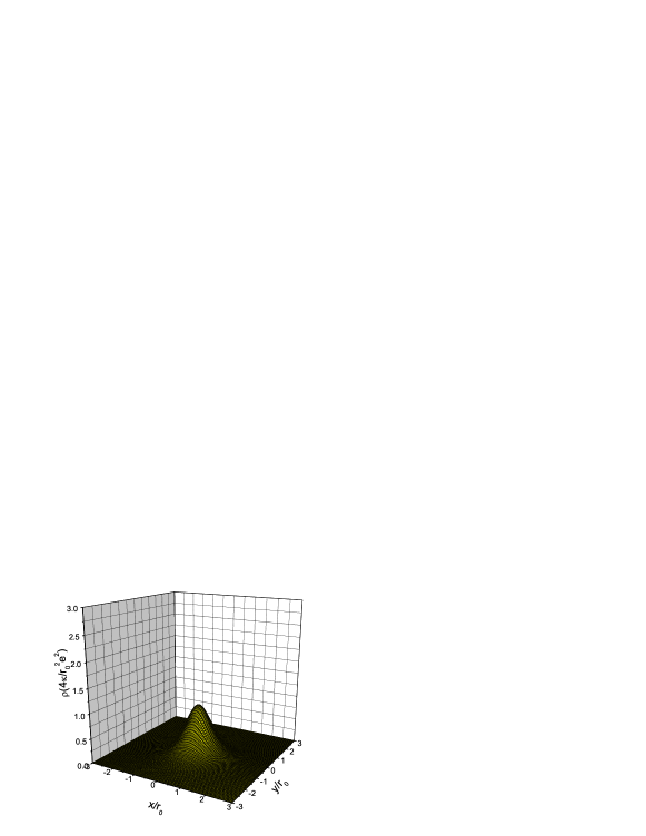
Figure 1: Density $\rho$ for a radially symmetric solution (33) representing one vortex with $Q=0$.($x\neq 0,y\neq 0,\hbar=c=1,\kappa>0$).

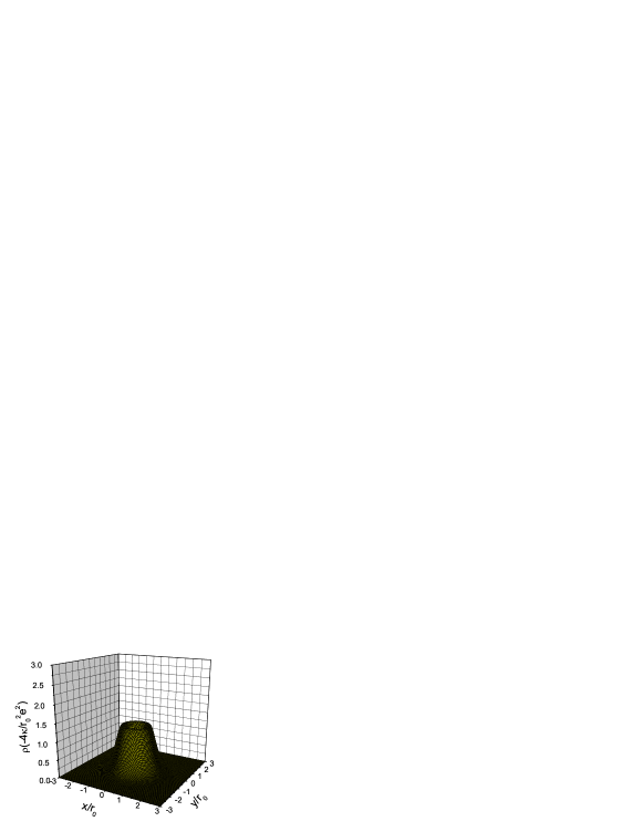
Figure 2: Density $\rho$ for a radially symmetric solution (33) representing one vortex with $Q=1$.($\kappa<0,\hbar=c=1$)

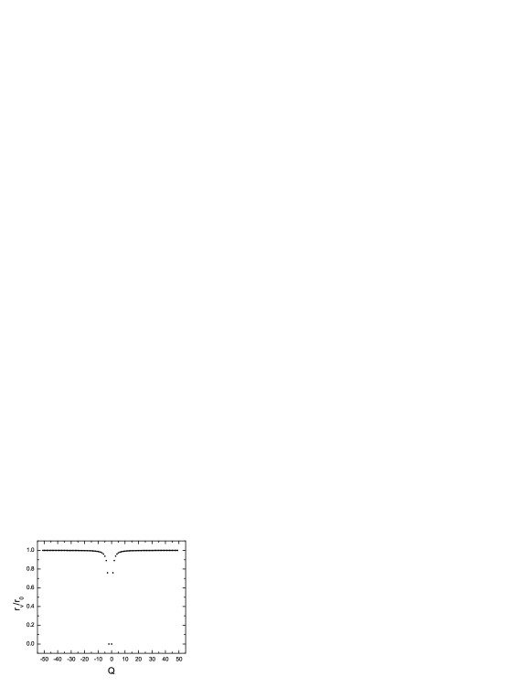
Figure 3: The values of radius of the vortex as $Q$ is varied when $\kappa<0$.($\hbar=c=1$)

Figure 4: The values of the height of the vortex as $Q$ is varied when $\kappa<0$.($\hbar=c=1$)

References

• (1) S. S. Chern, J. Simons, Proc. Nat. Acad. Sci. USA 68(4) (1971) 791; S. S. Chern, J. Simon,Ann. Math.99 (1974) 48.
• (2) E. Witten, Commun. Math. Phys. 121 (1989) 351.
• (3) S. Deser, R. Jackiw and S. Templeton, Phys. Rev. Lett.48 (1982) 975. S. Deser, R. Jackiw and S. Templeton, Ann. of Physics 140 (1982) 372.
• (4) R. Jackiw and E. J. Weinberg, Phys. Rev. Lett. 64 (1990) 2234.
• (5) R. Jackiw and S. Y. Pi, Phys. Rev. Lett. 64 (1990) 2969.
• (6) R. Jackiw and S. Pi, Phys. Rev.D 42 (1990) 3500.
• (7) J. Hong, Y. Kim and P. Y. Pac, Phys. Rev. Lett. 64 (1990) 2230.
• (8) S. M. Girvin and A.H. MacDonald, Phys. Rev. Lett. 58 (1987) 1252.
• (9) S.C. Zhang, T.H. Hansson and S. Kivelson, Phys. Rev. Lett. 62 (1988) 82.
• (10) V. Kalmeyer and R. B. Laughlin, Phys. Rev. Lett.59 (1987) 2095.
• (11) R. B. Laughlin, Phys. Rev. Lett. 60 (1988) 2677.
• (12) A. Achucarro and P.K. Townsend , Phys. Lett. B 180 (1986) 89.
• (13) E. Witten, Chern CSimons gauge theory as a string theory, in: The Floer Memorial Volume, in: Progress in Mathematics, vol. 133, Birkhauser, Boston, MA, 1995, pp. 637 C678. arXiv:hep-th/9207094.
• (14) E. Witten, Nucl. Phys.B 311 (1988) 46.
• (15) A. A. Abrikosov, Sov.Phys. JETP 5 (1957) 1174.
• (16) Bogomol nyi, E.B.: The stability of classical solutions. Sov. J. Nucl. Phys. 24 (1976) 449.
• (17) H. Nielsen and P. Olesen, Nucl. Phys. B 61 (1973) 45.
• (18) H. J. de Vega and F. Schaposnik, Phys. Rev. Lett. 56 2564 (1986); Phys. Rev. D 34 (1986) 3206.
• (19) N.Manton, Nucl. Phys. B 400 (1993) 624.
• (20) Y. S. Duan, M. L. Ge, Sci. Sin. 11 (1979) 1072; Y. S. Duan and X. H. Meng, J. Math.Phys. 34 (1993) 1149.
• (21) Y. S. Duan, G. H. Yang, and Y. Jiang, Gen. Rel. Grav. 29 715 (1997).
• (22) Y. S. Duan: SALC-PUB-3301(1984).
• (23) Y. S. Duan and X. G. Lee, Helv.Phys.Acta.58 (1995) 513.
• (24) X. G. Lee, M. Baldo and Y. S. Duan, Gen. Rel. Grav.29 (1997) 715.
• (25) H. Hopf, Math. Ann.96 (1929) 209.
• (26) G. V. Dunne, arXiv:hep-th/9902115.
• (27) A. S. Achwarz, Topology for Physicists. Springer-Verlag, Berlin,1994.
Refer to caption