hep-th/0604135

Giant Magnons

Diego M. Hofman^a and Juan Maldacena^b

^a Joseph Henry Laboratories, Princeton University, Princeton, NJ 08544, USA

^d Institute for Advanced Study, Princeton NJ 08540, USA.

Abstract

Studies of ${\cal N}=4$ super Yang Mills operators with large R-charge have shown that, in the planar limit, the problem of computing their dimensions can be viewed as a certain spin chain. These spin chains have fundamental “magnon” excitations which obey a dispersion relation that is periodic in the momentum of the magnons. This result for the dispersion relation was also shown to hold at arbitrary ’t Hooft coupling. Here we identify these magnons on the string theory side and we show how to reconcile a periodic dispersion relation with the continuum worldsheet description. The crucial idea is that the momentum is interpreted in the string theory side as a certain geometrical angle. We use these results to compute the energy of a spinning string. We also show that the symmetries that determine the dispersion relation and that constrain the S-matrix are the same in the gauge theory and the string theory. We compute the overall S-matrix at large ’t Hooft coupling using the string description and we find that it agrees with an earlier conjecture. We also find an infinite number of two magnon bound states at strong coupling, while at weak coupling this number is finite.

1 Introduction

String theory in $AdS_{5}\times S^{5}$ should be dual to ${\cal N}=4$ Yang Mills [1, 2, 3]. The spectrum of string states should be the same as the spectrum of operators in the Yang Mills theory. One interesting class of operators are those that have very large charges [4]. In particular, we consider operators where one of the SO(6) charges, $J$, is taken to infinity. We study states which have finite $E-J$. The state with $E-J=0$ corresponds to a long chain (or string) of $Z$s, namely to the operator $Tr[Z^{J}]$. We can also consider a finite number of other fields $W$ that propagate along this chain of $Z$s. In other words we consider operators of the form

$$O_{p}\sim\sum_{l}e^{i{lp}}(\cdots ZZZWZZZ\cdots)$$ (1.1)

where the field $W$ is inserted at position $l$ along the chain. On the gauge theory side the problem of diagonalizing the planar Hamiltonian reduces to a type of spin chain [5, 6], see [7] for reviews and further references. In this context the impurities, $W$, are “magnons” that move along the chain.

Using supersymmetry, it was shown that these excitations have a dispersion relation of the form [9]

$$E-J=\sqrt{1+{\lambda\over\pi^{2}}\sin^{2}{p\over 2}}$$ (1.2)

Note that the periodicity in $p$ comes from the discreteness of the spin chain. The large ’t Hooft coupling limit of this result is

$$E-J={\sqrt{\lambda}\over\pi}\left|\sin{p\over 2}\right|$$ (1.3)

Since this is a strong coupling result, it should be possible to reproduce it on the string theory side. At first sight it would seem that such a dispersion relation would require the string worldsheet to be discrete. In fact, this is not the case. We will show how to recover (1.3) on the string theory side with the usual strings moving in $AdS_{5}\times S^{5}$. The key element is that $p$ becomes a geometrical angle which will explain the periodic result. Thus we are able to identify the elementary excitations of the spin chain on the string theory side in an explicit fashion. The identification of these magnons allows us to explain, from the gauge theory side, the energy spectrum of the string spinning on $S^{5}$ which was considered in [11].

We will discuss the presence of extra central charges in the supersymmetry algebra which match the gauge theory analysis in [9]. Having shown that the two algebras match, then the full result (1.2) follows. Moreover, as shown in [9] the symmetry algebra constrains the $2\to 2$ $S$ matrix for these excitations up to an overall phase. This $S$ matrix is the asymptotic S-matrix discussed in [31]. It should be emphasized that these magnons are the fundamental degrees of freedom in terms of which we can construct all other states of the system. Integrability [30, 29, 23] implies that the scattering of these excitations is dispersionless. We check that this is indeed the case classically and we compute the classical time delay for the scattering process. This determines the large ’t Hooft coupling limit of the scattering phase. The final result agrees with the large $\lambda$ limit of [12]. This is done by exploiting a connection with the sine Gordon model [25, 26]. We also find that at strong coupling there is an infinite number of bound states of two magnons. These bound states have more energy than the energies of the individual magnons.

This article is organized as follows. In section 2 we explain the string theory picture for the magnons. We start by defining a particular limit that lets us isolate the states we are interested in. We continue with a review of gauge theory results in this limit. Then we find solutions of the classical sigma model action which describe magnons. We present these solutions in various coordinate systems. We also explain how the symmetry algebra is enhanced by the appearance of extra central charges, as in the gauge theory side [9]. Finally, we end by applying these results to the computation of the energy of a spinning string configuration in $S^{5}$ considered in [2]. In section 3 we compute the S-matrix at strong coupling and we analyze the bound state spectrum.

In appendix A we give some details on the supersymmetry algebra. In appendix B give some more details on the spectrum of bound states.

2 Elementary excitations on an infinite string

2.1 A large $J$ limit

Let us start by specifying the limit that we are going to consider. We will first take the ordinary ’t Hooft limit. Thus we will consider free strings in $AdS_{5}\times S^{5}$ and planar diagrams in the gauge theory. We then pick a generator $J=J_{56}\subset so(6)$ and consider the limit when $J$ is very large. We will consider states with energies $E$ (or operators with conformal dimension $\Delta=E$) which are such that $E-J$ stays finite in the limit. We keep the ’t Hooft coupling $\lambda\equiv g^{2}N$ fixed. This limit can be considered both on the gauge theory and the string theory sides and we can interpolate between them by varying the ’t Hooft coupling after having taken the large $J$ limit. In addition, when we consider an excitation we will keep its momentum $p$ fixed. In summary, the limit that we are considering is

$$J \to \infty~{},~{}~{}~{}~{}~{}~{}~{}~{}\lambda=g^{2}N={\rm fixed}$$ (2.4)

$$p = {\rm fixed}~{},~{}~{}~{}~{}~{}E-J={\rm fixed}$$ (2.5)

This differs from the plane wave limit [4] in two ways. First, here we are keeping $\lambda$ fixed, while in [4] it was taken to infinity. Secondly, here we are keeping $p$ fixed, while in [4] $n=pJ$ was kept fixed.

One nice feature of this limit is that it decouples quantum effects, which are characterized by $\lambda$, from finite $J$ effects, or finite volume effects on the string worldsheet.

Also, in this limit, we can forget about the momentum constraint and think about single particle excitations with non-zero momentum. Of course, when we take $J$ large but finite, we will need to reintroduce the momentum constraint.

2.2 Review of gauge theory results

In this subsection we will review the derivation of the formula (1.2). This formula could probably have been obtained in [8] had they not made a small momentum approximation at the end. This formula also emerged via perturbative computations [7]. A heuristic explanation was given in [14], which is very close to the string picture that we will find below. Here we will follow the treatment in [9] which exploits some interesting features of the symmetries of the problem.

The ground state of the system, the state with $E-J=0$, preserves 16 supersymmetries. These supercharges, which have $E-J=0$, act linearly on the impurities or magnons. They transform as $(2,1,2,1)+(1,2,1,2)$ under $SU(2)_{S^{5},L}\times SU(2)_{S^{5},R}\times SU(2)_{AdS_{5},L}\times SU(2)_{AdS_{5},R}$ where the various $SU(2)$ groups corresponds to the rotations in $AdS_{5}$ and $S^{5}$ which leave $Z$ invariant. These supercharges are the odd generators of two $SU(2|2)$ groups. The energy $\epsilon\equiv E-J$ is the (non-compact) $U(1)$ generator in each of the two $SU(2|2)$ supergroups. In other words, the two $U(1)$s of the two $SU(2|2)$ groups are identified. A single impurity with $p=0$ transforms in the smallest BPS representation of these two supergroups. In total, the representation has $8$ bosons plus $8$ fermions. This representation is BPS because its energy is $\epsilon=E-J=1$ which follows from the BPS bound that links the energy to the $SU(2)^{4}$ charges of the excitations. Let us now consider excitations with small momentum $p$. At small $p$ we can view the dispersion relation as that of a relativistic theory. Note that as we add a small momentum, the energy becomes higher but we still expect to have 8 bosons plus 8 fermions and not more, as it would be the case for representations of $SU(2|2)^{2}$ with $\epsilon>1$. What happens is that the momentum appears in the right hand side of the supersymmetry algebra. This ensures that the representation is still BPS. In fact, for finite $p$ there are two central charges [9]. These extra generators add or remove $Z$s to the left or right of the excitation and they originate from the commutator terms in the supersymmetry transformation laws, namely terms like $\delta W\sim\psi+[Z,\chi]$, see [9]. These extra central charges are zero for physical states with finite $J$ since we will impose the momentum constraint.

The full final algebra has thus three “central” generators in the right hand side, they are the energy $\epsilon$ and two extra charges which we call $k^{1},k^{2}$. Together with the energy these charges can be viewed as the three momenta $k^{\mu}$ of a 2+1 dimensional Poincare superalgebra. This is the same as the 2+1 dimensional Poincare superalgebra recently studied in [15, 16], we will see below that this is not a coincidence. Notice that the Lorentz generators are an outer automorphism of this algebra but they are not a symmetry of the problem we are considering. See appendix A for a more detailed discussion of the algebra.

As explained in [9] the expression for the “momenta” is $k^{1}+ik^{2}=h(\lambda)(e^{ip}-1)$ and similarly for the complex conjugate. This then implies that we have the formula

$$E-J=k^{0}=\sqrt{1+|k_{1}+ik_{2}|^{2}}=\sqrt{1+f(\lambda)\sin^{2}{p\over 2}}$$ (2.6)

The function $f(\lambda)$ is not determined by this symmetry argument. We know that $f(\lambda)={\lambda\over\pi}$ up to three loops in the gauge theory [5, 17] and that it is also the same at strong coupling (where it was checked at small momenta in [4]). [8] claims to show it is exactly $f={\lambda\over\pi}$ for all values of the coupling, but we do not fully understand the argument.

In the plane wave matrix model [4, 10] one can also use the symmetry algebra to determine a dispersion relation as in (2.6) and the function $f(\lambda)$ is nontrivial. More precisely, large $J$ states in the plane wave matrix model have an $SU(2|2)$ group (extended by the central charges to a 2+1 Poincare superalgebra) that acts on the impurities.

The conclusion is that elementary excitations moving along the string are BPS under the 16 supersymmetries that are linearly realized. Supersymmetry then ensures that we can compute the precise mass formula once we know the expression for the central charges.

2.3 String theory description at large $\lambda$

We will now give the description of the elementary impurities or elementary magnons at large $\lambda$ from the string theory side. In this regime we can trust the classical approximation to the string sigma model in $AdS_{5}\times S^{5}$.

In order to understand the solutions that we are going to study, it is convenient to consider first a string in flat space. We choose light cone gauge, with $X^{+}=\tau$, and consider a string with large $P_{-}$. The solution with $P_{+}=0$ corresponds to a lightlike trajectory with $X^{-}=$constant, see figure 1(a,c). Now suppose that we put two localized excitations carrying worldsheet momentum $p$ and $-p$ respectively. Let us suppose that at some instant of time these are on opposite points of the worldsheet spatial circle, see figure 1(b). We want to understand the spacetime description of such states. It is clear that the region to the left of the excitations and the region to the right will be mapped to the same lightlike trajectories with $X^{-}=$constant that we considered before. The important point is that these two trajectories sit at different values of $X^{-}$. This can be seen by writing the Virasoro constraint as

$$\partial_{\sigma}X^{-}=2\pi\alpha^{\prime}T_{\tau\sigma}~{},~{}~{}~{}~{}~{}~{}~{}~{}\Delta X^{-}=2\pi\alpha^{\prime}\int d\sigma T_{\tau\sigma}=2\pi\alpha^{\prime}p$$ (2.7)

where $T_{\tau\sigma}$ is the worldsheet stress tensor of the transverse excitations and we have integrated across the region where the excitation with momentum $p$ is localized. Thus the final spacetime picture is that we have two particles that move along lightlike trajectories that are joined by a string. At a given time $t$ the two particles move at the speed of light separated by $\Delta X^{1}|_{t}=\Delta X^{-}|_{X^{+}}=2\pi\alpha^{\prime}p$ and joined by a string, see figure 1(d). Of course, the string takes momentum from the leading particle and transfers it to the trailing one. On the worldsheet this corresponds to the two localized excitations moving toward each other. As the worldsheet excitations pass through each other the trailing particle becomes the leading one, see figure 1(c). For a closed string $X^{-}$ should be periodic, which leads to the momentum constraint $p_{total}=0$.

In the limit of an infinite string, or infinite $P_{-}$, we can consider a single excitation with momentum $p$ along an infinite string. Then the spacetime picture will be that of figure 2 where we have two lightlike trajectories, each carrying infinite $P_{-}$, separated by $\Delta X^{-}\sim p$ which are joined by a string. There is some $P_{-}$ being transferred from the first to the second. But since $P_{-}$ was infinite this can continue happening for ever. The precise shape of the string that joins the two points depends on the precise set of transverse excitations that are carrying momentum $p$.

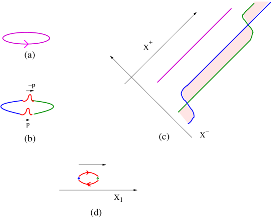
Figure 1: Localized excitations propagating along the flat space string worldsheet in light cone gauge. (a) Worldsheet picture of the light cone ground state, with $P_{+}=0$. (b) Worldsheet picture of two localized excitations with opposite momenta propagating along the string. (c) Spacetime description of the configurations in (a) and (b). The configuration in (a) gives a straight line at a constant $X^{-}$. The configuration in (b) gives two straight lines at constant $X^{-}$ when the localized excitations are separated on the worldsheet. When the two excitations in (b) cross each other the lines move in $X^{-}$. (d) Snapshot of the spacetime configuration in (b), (c) at a given time $t$.

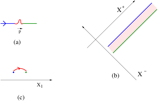
Figure 2: Localized excitations propagating on an infinite string. (a) Worldsheet picture of a localized excitation propagating along the string. (b) Spacetime behavior of the state in lightcone coordinates. We have two lightlike lines with a string stretching between them. (c) Snapshot of the state at a given time. The configuration moves to the right at the speed of light.

Armed with the intuition from the flat space case, we can now go back to the $AdS_{5}\times S^{5}$ case. We write the metric of $S^{5}$ as

$$ds^{2}=\sin^{2}\theta d\varphi^{2}+d\theta^{2}+\cos^{2}\theta d\Omega_{3}^{2}$$ (2.8)

where $\varphi$ is the coordinate that is shifted by $J$. The string ground state, with $E-J=0$, corresponds to a lightlike trajectory that moves along $\varphi$, with $\varphi-t$=constant, that sits at $\theta=\pi/2$ and at the origin of the spatial directions of $AdS_{5}$.

We can find the solution we are looking for in various ways. We are interested in finding the configuration which carries momentum $p$ with least amount of energy $\epsilon=E-J$. For the moment let us find a solution with the expected properties and we will later show that it has the minimum amount of energy for fixed $p$. We first pick a pair of antipodal points on $S^{3}$ so that, together with the coordinate $\theta$ and $\varphi$ they form an $S^{2}$. After we include time, the motion takes place in $R\times S^{2}$. We can now write the Nambu action choosing the parametrization

$$t=\tau~{},~{}~{}~{}~{}~{}~{}~{}~{}~{}\varphi-t=\varphi^{\prime}$$ (2.9)

and we consider a configuration where $\theta$ is independent of $\tau$. We then find that the action reduces to

$$S={\sqrt{\lambda}\over 2\pi}\int dtd\varphi^{\prime}\sqrt{\cos^{2}\theta{\theta^{\prime}}^{2}+\sin^{2}\theta}$$ (2.10)

It is easy to integrate the equations of motion and we get

$$\sin\theta={\sin\theta_{0}\over\cos\varphi^{\prime}}~{},~{}~{}~{}~{}~{}~{}-({\pi\over 2}-\theta_{0})\leq\varphi^{\prime}\leq{\pi\over 2}-\theta_{0}$$ (2.11)

where $0\leq\theta_{0}\leq\pi/2$ is an integration constant. See figure 3. In these variables the string has finite worldsheet extent, but the regions near the end points are carrying an infinite amount of $J$. We see that for this solution the difference in angle between the two endpoints of the string at a given time $t$ is

$$\Delta\varphi^{\prime}=\Delta\varphi=2({\pi\over 2}-\theta_{0})$$ (2.12)

It is also easy to compute the energy

$$E-J={\sqrt{\lambda}\over\pi}\cos\theta_{0}={\sqrt{\lambda}\over\pi}\sin{\Delta\varphi\over 2}$$ (2.13)

We now propose the following identification for the momentum $p$

$$\Delta\varphi=p$$ (2.14)

We will later see more evidence for this relation. Once we use this relation (2.13) becomes

$$E-J={\sqrt{\lambda}\over\pi}\left|\sin{p\over 2}\right|$$ (2.15)

in perfect agreement with the large $\lambda$ limit (1.3) of the gauge theory result (1.2). The sign of $p$ is related to the orientation of the string. In other words, $\Delta\varphi$ is the angular position of the endpoint of the string minus that of the starting point and it can be negative.

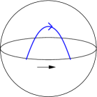
Figure 3: Giant magnon solution to the classical equations. The momentum of the state is given by the angular distance between the endpoints of the string. We depicted a configuration with $0<p<\pi$. A configuration with negative momentum would look the same except that the orientation of the string would be reversed. The string endpoints are on the equator and the move at the speed of light.

In order to make a more direct comparison with the gauge theory it is useful to pick a gauge on the worldsheet in such a way that, for the string ground state (with $E-J=0$), the density of $J$ is constant. There are various ways of doing this. One specific choice would be the light cone gauge introduced in [19]. We will now do something a bit different which can be done easily for strings on $R\times S^{2}$ and which will turn out useful for our later purposes. This consists in choosing conformal gauge and setting $t=\tau$. $x$ labels the worldsheet spatial coordinate. In this gauge the previous solution takes the form

$$\cos\theta = {\cos\theta_{0}\over\cosh\left[{x-\sin\theta_{0}t\over\cos\theta_{0}}\right]}={\sin{p\over 2}\over\cosh\left[{x-\cos{p\over 2}t\over\sin{p\over 2}}\right]}$$ (2.16)

$$\tan(\varphi-t) = \cot\theta_{0}\,\tanh\left[{x-\sin\theta_{0}t\over\cos\theta_{0}}\right]=\tan{p\over 2}\,\tanh\left[{x-\cos{p\over 2}t\over\sin{p\over 2}}\right]$$

where we used (2.14). In this case we see that the range of $x$ is infinite. These coordinates have the property that the density of $J$ away from the excitation is constant. This property allows us a to make an identification between the coordinate $x$ and the position $l$ (see (1.1)) along the chain in the gauge theory. More precisely, we compute the density of $J$ per unit $x$ in order to relate $l$ and $x$

$${dJ\over dx}={\sqrt{\lambda}\over 2\pi}~{}~{}~{}~{}~{}~{}~{}{\rm or}~{}~{}~{}~{}~{}~{}~{}dl={\sqrt{\lambda}\over 2\pi}dx$$ (2.17)

This relation allows us to check the identification of the momentum (2.14) since the relation between energy and momentum (1.3) determines the velocity in the gauge theory through the usual formula

$$v_{gauge}={dl\over dt}={d\epsilon(p)\over dp}={\sqrt{\lambda}\over 2\pi}\cos{p\over 2}~{},~{}~{}~{}~{}~{}~{}~{}~{}~{}{\rm for}~{}~{}~{}~{}p>0$$ (2.18)

On the other hand we see from (2.16) that the velocity is

$$v_{string}={dx\over dt}=\sin\theta_{0}=\cos{\Delta\varphi\over 2}$$ (2.19)

We see that after taking into account (2.17) the two velocities become identical if we make the identification (2.14).

The solution becomes simpler if expressed in terms of the coordinates introduced in [20]. Those coordinates were specially adapted to describe 1/2 BPS states which carry charge $J$. So it is not surprising that they are also useful for describing small excitations around such states. The $AdS_{5}\times S^{5}$ metric in those coordinates is a fibration of $R$, characterizing the time direction, and two $S^{3}$s (coming form $AdS_{5}$ and $S^{5}$) over a three dimensional space characterized by coordinates $x_{1},x_{2},y$. The plane $y=0$ is special because one of the two 3-spheres shrinks to zero size in a smooth way. Thus the plane $y=0$ is divided into regions (or “droplets”) where one or the other $S^{3}$ shrinks to zero size. The $AdS_{5}\times S^{5}$ solution contains a single circular droplet of radius $R$ where the $S^{3}$ coming from $AdS_{5}$ shrinks, see figure 4. Particles carrying $E-J=0$ live on the boundary of the two regions. In fact the circle constituting the boundary of the two regions sits at $\theta=\pi/2$ and it is parameterized by $\varphi^{\prime}=\varphi-t$ in previous coordinates. We will be only interested in the metric on this special plane at $y=0$ which takes the form, for $r<1$,

$$ds^{2}=R^{2}\left\{-(1-r^{2})\left[dt-{r^{2}\over(1-r^{2})}d\varphi^{\prime}\right]^{2}+{dr^{2}+r^{2}d{\varphi^{\prime}}^{2}\over(1-r^{2})}+(1-r^{2})d\Omega_{3}^{2}+\cdots\right\}$$ (2.20)

where $r^{2}=\sin^{2}\theta=x_{1}^{2}+x_{2}^{2}$ and the dots remind us that we are ignoring the $y$ coordinate and the second sphere, which has zero size at $y=0$ for $r\leq 1$.

In these coordinates the solution is simply a straight line that joins two points of the circle as shown in figure 4(a). This can be seen from (2.11), which can be rewritten as

$$r\cos\varphi^{\prime}=x_{1}={\rm const}$$ (2.21)

The energy is simply the length of the string measured with the flat metric on the plane parameterized by $x_{1},x_{2}$; $ds^{2}_{flat}=R^{2}(dx_{1}^{2}+dx_{2}^{2})$. In fact, the picture we are finding here is almost identical to the one discussed from the gauge theory point of view in [14]. If we restrict the arguments in [14] to 1/2 BPS states and their excitations we can see how this picture emerges from the gauge theory point of view. Namely, we first diagonalize the matrix $Z$ in terms of eigenvalues. Then the impurity is an off diagonal element of a second matrix $W$ which joins two eigenvalues that are at different points along the circle. The energy formula follows from the commutator term $tr|[Z,W]|^{2}$ in the gauge theory, see [14] for more details.

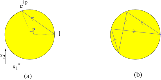
Figure 4: Giant magnons in LLM coordinates (2.20). (a) A giant magnon solution looks like a straight stretched string. It’s momentum $p$ is the angle subtended on the circle. $k_{1}$ and $k_{2}$ are the projections of the string along the directions $\hat{1}$ and $\hat{2}$. The direction of the string gives the phase of $k_{1}+ik_{2}$, while its length gives the absolute value of the same quantity. (b) A closed string state built of magnons that are well separated on the worldsheet. Notice that the total central charges $k_{1},~{}k_{2}$ vanish. Similarly the total angle subtended by the string, which is the total momentum $p_{total}$ also vanishes modulo $2\pi$.

These coordinates are very useful for analyzing the symmetries. In particular, we will now explain the appearance of extra central charges and we will match the superalgebra to the one found on the gauge theory side in [9]. Under general considerations we know that the anticommutator of two supersymmetries in 10 dimensional supergravity contains gauge transformations for the NS-$B_{2}$ field [21]. These act non-trivially on stretched strings. In flat space this leads to the fact that straight strings are BPS. In fact, inserting the explicit expression of the Killing spinors in [20] into the general formula for the anticommutator of two supercharges [21] it is possible to see that the relevant NS gauge transformations are those with a constant gauge parameter $\Lambda_{1},~{}\Lambda_{2}$, $\delta B=d\Lambda$ . Strings that are stretched along the $\hat{1}$ or $\hat{2}$ directions acquire a phase under such gauge transformations. Thus these are the central charges that we are after. Note that in order to activate these central charges it is not necessary to have a compact circle in the geometry. In fact, the string stretched between two separated D-branes in flat space is BPS for the same reason.

Actually, the supersymmetry algebra is identical to a supersymmetry algebra in 2+1 dimensions, where the string winding charges, $k^{1},k^{2}$, play the role of the spatial momenta. See appendix A for more details on the algebra. From the 2+1 dimensional point of view it is a peculiar Poincare super algebra since it has $SO(4)^{2}$ charges in the right hand side of supersymmetry anti-commutators. Of course, this is the same supersymmetry algebra that appeared in the gauge theory discussion [9]. In conclusion, the symmetry algebra is exactly the same on both sides. The extra central charges are related to string winding charges. We can think of the vector given by the stretched string as the two spatial momenta $k^{1},~{}k^{2}$ appearing in the Poincare superalgebra. In other words, we can literally think of the stretched string in figure 4 as specifying a vector $k^{1},k^{2}$ of size

$$k^{1}+ik^{2}={R^{2}\over 2\pi\alpha^{\prime}}(e^{ip}-1)=i{\sqrt{\lambda}\over\pi}e^{i{p\over 2}}\sin{p\over 2}$$ (2.22)

Then the usual relativistic formula for the energy implies (2.6), as in the gauge theory. Note that the problem we are considering does not have lorentz invariance in 2+1 dimensions. Lorentz invariance is an outer automorphism of the algebra, that is useful for analyzing representations of the algebra, but it is not an actual symmetry of the theory. In particular, in our problem the formula (2.6) is not a consequence of boost invariance, since boosts are not a symmetry. It is a consequence of supersymmetry, it is a BPS formula. Note that rotations of $k^{1},~{}k^{2}$ are indeed a symmetry of the problem and they correspond to rotations of the circle in figure 4. This is the symmetry generated by $J$. Note also that a physical state with large but finite $J$ will consist of several magnons but the configurations should be such that we end up with a closed string, see figure 4(b) . Thus, for ordinary closed strings the total value of the central charges is zero, since there is no net string winding. This implies, in particular, that for a closed finite $J$ string there are no new BPS states other than the usual ones corresponding to operators $Tr[Z^{J}]$.

Notice that the classical string formula (2.13) is missing a 1 in the square root as compared to (1.2). This is no contradiction since we were taking $p$ fixed and $\lambda$ large when we did the classical computation. This 1 should appear after we quantize the system. In fact, for small $p$ and $\lambda$ large, we can make a plane wave approximation and, after quantization, we recover the 1 [22, 4]. But if we did not quantize we would not get the 1, even in the plane wave limit. So we see that in the regime that the 1 is important we indeed recover it by doing the semiclassical quantization. This 1 is also implied by the supersymmetry algebra. The argument is identical to the one in [9] once we realize that the central charges are present and we know the relation between the central charges and the momentum $p$, as in (2.22). Notice that the classical solutions we discussed above break the $SO(4)$ symmetry since they involve picking a point on $S^{3}\subset S^{5}$ where the straight string in figure 4(a) is sitting. Upon collective coordinate quantization we expect that the string wavefunction will be constant on this $S^{3}$. In addition, we expect to have fermion zero modes. They originate from the fact that the magnon breaks half of the 16 supersymmetries that are left unbroken by the string ground state. Thus we expect 8 fermion zero modes, which, after quantization, will give rise to $2^{4}=16$ states, 8 fermions + 8 bosons. This argument is correct for fixed $p$ and large $\lambda$. In fact, all these arguments are essentially the same as the ones we would make for a string stretching between two D-branes. Notice that all magnons look like stretched strings in the $S^{5}$ directions, as in figure 4(a), including magnons corresponding to insertions of $\partial_{\mu}Z$ which parameterize elementary excitations along the $AdS_{5}$ directions. Of course, here we are considering a single magnon. Configurations with many magnons can have large excursions into the $AdS$ directions.

Since the stretched string solution in figure 4(a) is BPS, it is the minimum energy state for a given $p$.

In fact, we can consider large $J$ string states around other 1/2 BPS geometries, given by different droplet shapes as in [20]. In those cases, we will have BPS configurations corresponding to strings ending at different points on the boundary of the droplets and we have strings stretching between these points. It would be nice to see if the resulting worldsheet model is integrable.

Note that the fact that the magnons have a large size (are “giant”) at strong coupling is also present in the Hubbard model description in [44] .

Finally, let us point out that our discussion of the classical string solutions focussed on an $R\times S^{2}$ subspace of the geometry. Therefore, the same solutions will describe giant magnons in the plane wave matrix model [4, 10] and other related theories [15]. Similar solutions also exist in $AdS_{2,3}\times S^{2,3}$ with RR fluxes (NS-fluxes would change the equations already at the classical level).

2.4 Spinning folded string

In this subsection we apply the ideas discussed above to compute the energy of a spinning folded string considered in [11]. This is a string that rotates in an $S^{2}$ inside $S^{5}$. For small angular momentum $J$ this is a string rotating around the north pole. Here we are interested in the limit of large $J$ where the ends of the rotating string approach the equator, see figure 5. In this limit the energy of the string becomes [11]

$$E-J=2{\sqrt{\lambda}\over\pi}$$ (2.23)

This string corresponds to a superposition of two “magnons” each with maximum momentum, $p=\pi$. Notice that the dispersion relation implies that such magnons are at rest, see (2.18). They are equally spaced on the worldsheet. At large $J$ we can ignore the interaction between the “magnons” and compute the energy of the state as a superposition of two magnons. We see that the energy (2.23) agrees precisely with the energy of two magnons with $p=\pi$.

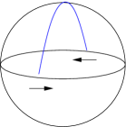
Figure 5: Spinning string configuration that corresponds to two magnons with $p=\pi$.

Since the $\lambda$ dependence of the strings spinning in AdS in [2] is somewhat similar, one might find an argument for that case too. In fact, the solutions we are considering here, such as the one in figure 4(b) is the sphere analog of the solutions with spikes considered in [45].

3 Semiclassical S-matrix

3.1 General constraints on the S-matrix

In this section we consider the S-matrix for scattering of two magnons. On the gauge theory side this is the so called “asymptotic S-matrix” discussed in [31]. In the string theory side it is defined in a similar way: we take two magnons and scatter them. Then, we define the $S$ matrix for asymptotic states as we normally do in 1+1 dimensional field theories. Since the sigma model is integrable [30, 29], we expect to have factorized scattering. It was shown in [23] that integrability still persists in the lightcone gauge (this was shown ignoring the fermions). In fact we will later check explicitly that our magnons undergo classical dispersionless scattering.

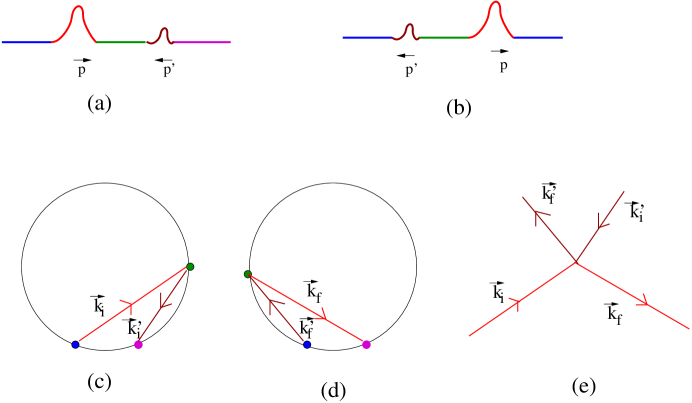
Figure 6: Scattering of $2\rightarrow 2$ magnons. (a) Worldsheet picture of asymptotic initial state. (b) Worldsheet picture of asymptotic final state. (c) Initial state in LLM coordinates. (d) Final state in LLM coordinates. (e) Initial and final configuration for the momenta $\vec{k}$ that are relevant for the 2+1 dimensional kinematics of the process.

As we mentioned above the supersymmetry algebra is the same in the gauge theory and the string theory. We have only shown here that the algebra is the same at the classical level on the string theory side. But it is very natural to think that after quantization we will still have the same algebra. Thus, any constraint coming from this algebra is the same. An important constraint for the $S$ matrix was derived by Beisert in [9]. Each of the magnons can be in one of 16 states (8 bosons plus 8 fermions). So the scattering matrix is a $16^{2}\times 16^{2}$ matrix. Beisert showed that this matrix is completely fixed by the symmetry up to an overall phase (and some phases that can be absorbed in field redefinitions). Schematically $S=\hat{S}_{ij}S_{0}$ where $\hat{S}_{ij}$ is a known matrix and $S_{0}$ is an unknown phase. The same result holds then for the string theory magnons. In fact, it was conjectured in [12, 31, 32] that the two S-matrices differ by a phase. Here we are pointing out that this structure is a consequence of the symmetries on the two sides. The fact that the whole $S$ matrix is determined up to a single function is analogous to the statement that the four particle scattering amplitude in ${\cal N}=4$ SYM is fixed up to a scalar function of the kinematic invariants. The reason is that two massless particles with 16 states each give a single massive, non-BPS, representation with $2^{8}=16^{2}$ states.

A two magnon scattering process has a kinematics that is shown in figure 6. Notice that we can literally think of the straight strings as determining the initial and final momentum vectors of the scattering process as in figure 6(e). The orientation of these vectors is important. The constraints on the matrix structure of the $S$ matrix are exactly the same as the constraints that a four particle scattering amplitude in a relativistic 2+1 dimensional field theory with the same superalgebra would have. These constraints are easy to derive in the center of mass frame. And we could then boost to a general frame. Notice that from the 2+1 dimensional point of view fermions have spin, and thus their states acquire extra phases under rotation. In other words, when we label a state by saying what its momentum $p$ is, we are just giving the magnitude of $\vec{k}$, but not its orientation. The orientation of $\vec{k}$ depends on the other magnons. For example, in the scattering process of figure 6(a,b) the initial and final states have the same momenta $p,p^{\prime}$, but the initial vectors ${\vec{k}}_{i},~{}{\vec{k}^{\prime}}_{i}$ have different orientation than the final vectors ${\vec{k}}_{f},~{}{\vec{k}^{\prime}}_{f}$. When we consider a sequence of scattering processes, one after the other, it is important to keep track of the orientation of $\vec{k}$. In other words, under an overall rotation the $S$ matrix is not invariant, it picks up some phases due to the fermion spins. In [9] these phases are taken into account by extra insertions of the field $Z$ which makes the chain “dynamic”.

Note that the constraints on the matrix structure of the scattering amplitude are applicable in a more general context to any droplet configuration of [20]. For example, it constrains the scattering amplitude for elementary excitations in other theories with the same superalgebra. Examples are the massive M2 brane theory [33] or the theories considered in [15, 16].

Note that the existence of closed subsectors is a property of factorized scattering (integrability) and the matrix structure of the $\hat{S}$ matrix, but does not depend on the precise nature of the overall phase. Thus closed subsectors exist on both sides. This argument shows this only in the large $J$ limit where the magnons are well separated and we can use the asymptotic $S$ matrix.

We expect that the overall phase, $S_{0}$, will interpolate between the weak and strong coupling results. The full interpolating function has not yet been determined.

In this section we will compute in a direct, and rather straightforward way, the semiclassical S-matrix for the scattering of string theory magnons. It turns out that the result will agree with the one derived in [12] through more indirect methods.

Notice that at large ’t Hooft coupling and fixed momentum, the approximate expression (1.3) amounts to a relativistic approximation to the non-relativistic formula (1.2). Similarly, in this limit, the matrix prefactor $\hat{S}$ becomes that of a relativistic theory and it is a bit simpler.

Notice that the theory in light cone gauge is essentially massive so that we can define scattering processes in a rather sharp fashion, in contrast with the full covariant sigma model which is conformal, a fact that complicates the scattering picture. Nevertheless, starting from the conformal sigma model can be a useful way to proceed [13].

3.2 Scattering phase at large $\lambda$ and the sine-Gordon connection

In the semiclassical limit where $\lambda$ is large and $p$ is kept fixed the leading contribution to the $S$ matrix comes from the phase $\delta$ in $S_{0}=e^{i\delta}$, which goes as $\delta\sim\sqrt{\lambda}f(p,p^{\prime})$. For fixed momenta, this phase dominates over the terms that come from the matrix structure $\hat{S}$ in the scattering matrix. In this section, we compute this phase, ignoring the matrix prefactor $\hat{S}$ in the S-matrix.

In the semiclassical approximation the phase shift can be computed by calculating the time delay that is accumulated when two magnons scatter. The computation is very similar to the computation of the semiclassical phase for the scattering of two sine Gordon solitons, as computed in [24]. In fact, the computation is almost identical because the magnons we discuss are in direct correspondence with sine Gordon solitons. This uses the relation between classical sine Gordon theory and classical string theory on $R\times S^{2}$ [25, 26]. It is probably also possible to obtain these results from [28], but we found it easier to do it using the correspondence to the sine Gordon theory. The map between a classical string theory on $R\times S^{2}$ and the sine Gordon model goes as follows. We consider the string action in conformal gauge and we set $t=\tau$. Then the Virasoro constraints become

$$1=\dot{\bf n}^{2}+{{\bf n}^{\prime}}^{2}~{},~{}~{}~{}~{}~{}\dot{\bf n}.{\bf n}^{\prime}=0$$ (3.24)

where ${\bf n}^{2}=1$ parameterizes the $S^{2}$. The equations of motion follow from these constraints. The sine Gordon field is defined via

$$\cos 2\phi=\dot{\bf n}^{2}-{{\bf n}^{\prime}}^{2}$$ (3.25)

For the “magnon” solution we had above we find that $\phi$ is the sine Gordon soliton

$$\tan{\phi\over 2}=\exp\left[{\cos{p\over 2}t-x\over\sin{p\over 2}}\right]=e^{-\gamma(x-vt)}~{},~{}~{}~{}~{}~{}~{}~{}~{}~{}v=\cos{p\over 2}~{},~{}~{}~{}~{}~{}~{}~{}~{}\gamma^{-2}=1-v^{2}$$ (3.26)

Notice that the energy of the sine Gordon soliton is inversely proportional to the string theory energy of the excitation (2.13)

$$E_{s.g.}={\gamma}=\cosh\hat{\theta}~{},~{}~{}~{}~{}~{}~{}~{}~{}~{}\epsilon_{magnon}={\sqrt{\lambda}\over\pi}\,{1\over\gamma}~{},~{}~{}~{}~{}~{}~{}~{}~{}~{}~{}~{}~{}~{}\cosh{\hat{\theta}}={1\over\sin{p\over 2}}$$ (3.27)

where we measure the sine Gordon energy relative to the energy of a soliton at rest and we introduced the sine Gordon rapidity ${\hat{\theta}}$. Note that a boost on the sine Gordon side translates into a non-obvious classical symmetry on the $R\times S^{2}$ side. Do not confuse this approximate boost symmetry of the sine Gordon theory with the boosts that appeared in our discussion of the supersymmetry algebra. Neither of them is a true symmetry of the problem, but they are not the same!.

We now consider a soliton anti-soliton pair and we compute the time delay for their scattering as in [24]. (If we use a soliton-soliton pair we obtain the same classical answer). Since the $x$ and $t$ coordinates are the same in the two theories, this time delay is precisely the same for the string theory magnons and for the sine Gordon solitons. The Sine Gordon scattering solution in the center of mass frame is

$$\tan{\phi\over 2}={1\over v}{\sinh\gamma vt\over\cosh\gamma x}$$ (3.28)

The fact that the sine Gordon scattering is dispersionless implies that the scattering of magnons is also dispersionless in the classical limit (of course we also expect it to be dispersionless in the quantum theory).

The time delay is

$$\Delta T_{CM}={2\over\gamma v}\log v$$ (3.29)

We now boost the configuration (3.28) to a frame where we have a soliton moving with velocity $v_{1}$ and an anti-soliton with velocity $v_{2}$, with $v_{1}>v_{2}$. Then the time delay that particle 1 experiences as it goes through particle 2 is

$$\Delta T_{12}={2\over\gamma_{1}v_{1}}\log v_{cm}$$ (3.30)

where $v$ is the velocity in the center of mass frame

$$2\log v_{cm}=2\log\tanh\left[{\hat{\theta}_{1}-\hat{\theta}_{2}\over 2}\right]=\log\left[{1-\cos{p_{1}-p_{2}\over 2}\over 1-\cos{p_{1}+p_{2}\over 2}}\right]~{},~{}~{}~{}~{}~{}{\rm for}~{}~{}~{}p_{1},~{}p_{2}>0$$ (3.31)

We can now compute the phase shift from the formula

$${\partial\delta_{12}(\epsilon_{1},\epsilon_{2})\over\partial\epsilon_{1}}=\Delta T_{12}$$ (3.32)

We obtain

$$\delta={\sqrt{\lambda}\over\pi}\left\{\left[-\cos{p_{1}\over 2}+\cos{p_{2}\over 2}\right]\log\left[{1-\cos{p_{1}-p_{2}\over 2}\over 1-\cos{p_{1}+p_{2}\over 2}}\right]\right\}-p_{1}{\sqrt{\lambda}\over\pi}\sin{p_{2}\over 2}$$ (3.33)

Note that, even though the time delay is identical to the sine Gordon one, the phase shift is different, due to the different expression for the energy (3.27). This implies, in particular, that the phase shift is not invariant under sine Gordon boosts. The first term in this expression agrees precisely with the large $\lambda$ limit of the phase in [12]. The second term in (3.33) looks a bit funny. However, we need to recall that the definition of this S-matrix is a bit ambiguous. This ambiguity is easy to see in the string theory side and was noticed before. For example [35] and [36] obtained different S-matrices for the scattering of magnons at low momentum (near plane wave limit). The difference is due to a different choice of gauge which translates into a different choice of worldsheet $x$ variable. In [35] the $x$ variable was defined in such a way that the density of $J$ is constant. In [36] it was defined so that the density of $E+J$ is constant. In our case we have defined it in such a way that the density of $E$ is constant, since we have set $\dot{t}=1$ in conformal gauge. All these choices give the same definition for the $x$ variable when we consider the string ground state. The difference lies in the different length in $x$ that is assigned to the magnons, which have $E-J\not=0$. Thus the $S$ matrix computed in different gauges will differ simply by terms of the form $e^{ip_{i}f(p_{j})}$ where $f(p_{j})$ is the difference in the length of the magnon on the two gauges. Of course the Bethe equations are the same in both cases since the total length of the chain is also different and this cancels the extra terms in the $S$ matrix. The position variable that is usually chosen on the gauge theory side assigns a length 1 to the impurity. At large $\lambda$ we can ignore 1 relative to $\lambda$ and say that the length of the impurity is essentially zero. Thus we can say that the gauge theory computation is using coordinates where the density of $J$ is constant. Using the relation between the gauge theory spatial coordinate $l$ and our worldsheet coordinate $x$ (2.17) (which is valid in the region where $E-J=0$) we get that the interval between of two points separated by a magnon are related by

$$\Delta l=\int dx{dJ\over dx}=\int dx{dE\over dx}-({dE\over dx}-{dJ\over dx})={2\pi\over\sqrt{\lambda}}\Delta x-\epsilon$$ (3.34)

where $\Delta l$ is the interval in the conventions of [12] and $\Delta x$ is the interval in our conventions. So we see that in our gauge the magnon will have an extra length of order $\epsilon(p)$. Thus $S_{string-Bethe}=S_{ours}e^{ip_{1}\epsilon_{2}}$, where $S_{string-Bethe}$ is the $S$ matrix in the conventions used in [12]. This cancels the last term in (3.33). In summary, after expressing the result in conventions adapted to the gauge theory computation we find that for $sign(\sin{p_{1}\over 2})>0$ and $sign(\sin{p_{2}\over 2})>0$ we get

$$\delta(p_{1},p_{2})=-{\sqrt{\lambda}\over\pi}(\cos{p_{1}\over 2}-\cos{p_{2}\over 2})\log\left[{\sin^{2}{p_{1}-p_{2}\over 4}\over\sin^{2}{p_{1}+p_{2}\over 4}}\right]$$ (3.35)

The cases where $p<0$ can be recovered by shifting $p$ by a period so that $\sin{2\pi+p\over 2}>0$. The function (3.35) should be trusted when $\sin{p_{i}\over 2}>0$ and it should be defined to be periodic with period $2\pi$ outside this range. Note that this function goes to zero when $p_{1}\to 0$ with $p_{2}$ fixed. When $p$ is small we need to quantize the system. We can check that, after quantization, the $S$ matrix is still trivial for small $p_{1}$ and fixed $p_{2}$. This can be done by expanding in small fluctuations around our soliton background. We find that the small excitations propagate freely through the soliton.

The leading answer (3.35) vanishes at small $p$. In fact, at small $p$ it is important to properly quantize the system and the result depends on the polarizations of the states, see [35]. For example, in the $SU(1|1)$ sector [35] found (see also [36])

$$S_{string}=-1+i{1\over 2}\left(p_{1}\sqrt{1+{\lambda\over 4\pi^{2}}p_{2}^{2}}-p_{2}\sqrt{1+{\lambda\over 4\pi^{2}}p_{1}^{2}}-p_{1}+p_{2}\right)$$ (3.36)

Corrections to the leading phase (3.35) were computed in [37] and some checks were made in [39, 38].

On the gauge theory side the phase is known up to three loop orders in $\lambda$ [17]. Of course, finding the full interpolating function is an outstanding challenge.

Finally, to complete the discussion of scattering states, we comment on the spacetime picture of the scattering process. In the classical theory, besides specifying $p$, we can also specify a point on $S^{3}$ for each of the two magnons that are scattering off each other. We do not know the general solution. The sine Gordon analysis we did above applies only if the point on $S^{3}$ is the same for the two magnons or are antipodal for the two magnons. In the first case we have a soliton-soliton scattering in the sine-Gordon model and in the second we have a soliton-anti-soliton scattering. Both give the same classical time delay. The soliton anti-soliton scattering with $p_{1}=-p_{2}$ looks initially like loop of string made of two magnons. One of the endpoints has infinite $J$ and the other has finite $J$. The point in the front, which initially carries a finite amount of $J$, looses all its $J$ and it moves to the left. The loop becomes a point and then the loops get formed again but with the finite $J$ point to the left, behind the point that carries infinite $J$. See figure 7. The soliton soliton scattering is represented by a doubly folded string that looks initially like a two magnon state. As time evolves the point in the front, which carries finite $J$, detaches from the equator and moves back of the other endpoint which carries infinite $J$. The final picture is, again, equivalent to the original one with front and back points exchanged. We see that in both cases asymptotic states are well defined and look like individual magnons.

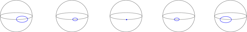
Figure 7: Evolution of the soliton anti-soliton scattering state. Time increases to the right. We have chosen a rotating frame on the sphere where the point with infinite $J$ is stationary. At $t=0$ the string is all concentrated at a point, the point that carries infinite $J$. The state looks asymptotically as two free magnons on opposite hemispheres and with the same endpoints.

3.3 Bound states

One interesting property of the sine Gordon theory is that it displays an interesting set of localized states which can be viewed as soliton-antisoliton bound states. The corresponding classical solutions are given by performing an analytic continuation $v\to ia$ in (3.28)

$$\tan{\phi\over 2}={1\over a}{\sin\gamma_{a}at\over\cosh\gamma_{a}x}~{},~{}~{}~{}~{}~{}~{}~{}\gamma_{a}^{-2}=1+a^{2}$$ (3.37)

In the semiclassical approximation to the sine-Gordon theory we can quantize these modes [24, 40]. These particles then appear as poles in the $S$ matrix, [41].

In this section we will use these sine Gordon solutions (3.37) in order to produce solutions representing bound states of magnons. We will then quantize them semiclassically.

We can start with the solution (3.37) and we boost it with a boost parameter $\gamma$. Then the soliton and anti-soliton components have rapidities

$$\hat{\theta}_{1,2}=\hat{\theta}\pm i\hat{\theta}_{a}~{},~{}~{}~{}~{}~{}~{}~{}v=\tanh{\hat{\theta}}~{},~{}~{}~{}~{}~{}~{}~{}~{}a=\tan{\hat{\theta}}_{a}$$ (3.38)

where $v$ characterizes the velocity of the bound state and $a$ is the parameter $a$ appearing in the center of mass frame solution (3.37). In the sine Gordon theory the energy is given by the sum of the energies of a soliton anti-soliton pair with these rapidities (3.38)

$$E^{bound}_{sg}=E(\hat{\theta}+i\hat{\theta}_{a})+E(\hat{\theta}-i\hat{\theta}_{a})=\cosh(\hat{\theta}+i\hat{\theta}_{a})+\cosh({\hat{\theta}}-i{\hat{\theta}}_{a})=2\cosh{\hat{\theta}}\cos{\hat{\theta}}_{a}$$ (3.39)

We can understand this formula as resulting from analytic continuation of the formula that gives a similar additive result for scattering states. Recall that (3.37) is a configuration obtained from a scattering solution (3.28) by analytically continuing the rapidities.

We now want to understand what these states correspond to in our system. From the string theory point of view we can label the states in terms of the momentum $p$ or in terms of the rapidity $\hat{\theta}$ related by (3.27). The localized solutions (3.37) should correspond to localized solutions on the worldsheet that come from analytically continuing the parameters of scattering solutions. Thus we expect that, also in the string theory, the energy will be a sum of the energies of its components

$$\epsilon^{bound}=\epsilon({\hat{\theta}}_{1})+\epsilon({\hat{\theta}}_{2})={\sqrt{\lambda}\over\pi}\left[{1\over\cosh{\hat{\theta}}_{1}}+{1\over\cosh{\hat{\theta}}_{2}}\right]$$ (3.40)

This expression for the energy is important for what we will do later. We have checked directly that starting with a boosted version of (3.37), inverting the equation (3.25), and computing the energies we get (3.40). See appendix B for more details. From the rapidities we can also define the momenta of each of the particles through the relation (3.27). These momenta are complex

$$p_{1,2}=p\pm iq~{},~{}~{}~{}~{}~{}~{}~{}~{}{1\over\cosh{\hat{\theta}}_{i}}=\sin{p_{i}\over 2}$$ (3.41)

We also see that the total momentum of the state is $P=2p$.

In order to semiclassically quantize these states we need to find the period of oscillation. This is the time it takes for the solution to look the same up to an overall translation. We find

$$T=2\pi{\gamma\over\gamma_{a}a}=2\pi{\cosh{\hat{\theta}}\over\sin{\hat{\theta}}_{a}}={2\pi}{1\over\tanh{q\over 2}}~{},~{}~{}~{}~{}~{}~{}~{}~{}{\rm note~{}that}~{}~{}~{}\tan{p\over 2}={\gamma_{a}\over v\gamma}$$ (3.42)

where we used (3.41). We now define the action variable $n$ which in the quantum theory should be an integer, through the equation

$$dn={T\over 2\pi}d\epsilon|_{p}={\sqrt{\lambda}\over\pi}\sin{p\over 2}\cosh{q\over 2}dq~{}~{}~{}~{}{\rm or}~{}~{}~{}n={2\sqrt{\lambda}\over\pi}\sin{p\over 2}\sinh{q\over 2}$$ (3.43)

where we keep the momentum fixed, which is another conserved quantity. We obtain

$$\epsilon={\sqrt{\lambda}\over\pi}(\sin{p_{1}\over 2}+\sin{p_{2}\over 2})={2\sqrt{\lambda}\over\pi}\sin{p\over 2}\cosh{q\over 2}=\sqrt{n^{2}+{4\lambda\over\pi^{2}}\sin^{2}{p\over 2}}$$ (3.44)

where we should trust this formula only for large $n$. So, in the regime where we can trust it, these states have more energy than two magnons each with momentum $p$. We do not see any sign of a breakdown in our analysis for very large $n$. So for large but finite $\lambda$ there is an infinite number of bound states. It looks like these bound states should belong to general massive representations of $SU(2|2)^{2}$ since those are the ones that generally correspond to a two magnon configuration.

Note that the bound states carry momentum $P=2p$ and that as $p$ varies from zero to $\pi$, $P$ varies from 0 to $2\pi$ and the two endpoints of the string move over the whole equator of the $S^{2}$. But the configuration is not periodic in $P$. Namely, for small $P$ we have a bound state of two magnons with small $p$, while for $P\sim 2\pi$ we have a bound state of two large magnons with $p\sim\pi$.

The spacetime picture of these solutions varies considerably depending on parameters $p$ and $q$. The easiest case to analyze is the solution corresponding to the breather at rest. This corresponds to choosing maximal $p=\pi$. These are strings with one fixed point ($\varphi-t=\textrm{const}$) which sweep the entire sphere as they evolve in time, see figure 8. At quarter the period they look like two magnons of maximal $p$. The value of $q$ controls the period of the sweep. Because $P=2p=2\pi$ for this case there is no distance between the endpoints of the string. As we decrease $p$ a gap opens up while the strings still sweep the sphere, see figure 9(a). At $p=\frac{\pi}{2}$ the gap is maximal and the solutions change character:they do not sweep the sphere any longer. For small $p$ the solution is bounded to a small region of the sphere, see figure 9(b). $q$ still controls the period. In appendix B, we discuss the relevant variables and calculate the energies of these solutions. It would be nice to find more explicit expressions for the solutions.

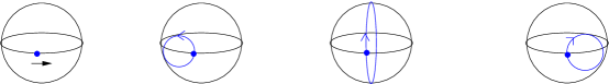
Figure 8: Evolution of the bound state with $p=\pi$. Time increases to the right. We have chosen a rotating frame on the sphere where the point with infinite $J$ is stationary. At $t=0$ the string is all concentrated at a point, the point that carries infinite $J$. As time progresses a loop forms, then this loop sweeps the whole sphere and becomes a point again. The motion repeats itself again except that the loop has the opposite orientation. Thus in each period we performs two sweeps of the sphere.

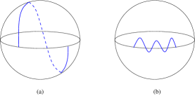
Figure 9: Snapshots of other string bound states. (a) Large p bound state. (b) Small p bound state.

We can now compare these results to the bound states at weak coupling. We focus on the $SU(2)$ sector for simplicity and to lowest order in the ’t Hooft coupling. In that case we simply have the XXX spin chain [5]. It is then easy to show by looking at the poles of the $S$ matrix that there is single bound state of two magnons. Writing the momenta as $p_{1,2}=p\pm iq$ one can check that the bound state has

$$q=\log(\cos p)$$ (3.45)

Using the dispersion relations for magnons we can check that the energy is

$$\epsilon=\epsilon(p_{1})+\epsilon(p_{2})=\sum_{i=1}^{2}1+{\lambda\over 2\pi^{2}}\sin^{2}{p_{i}\over 2}=2+{\lambda\over 2\pi^{2}}2\cos^{2}{p\over 2}\sin^{2}{p\over 2}$$ (3.46)

In this case we see that the energy is smaller than the sum of the energies of two magnons with momentum $p$. We also see that the size of the bound state goes to infinity, and the binding energy disappears, when $q\to 0$. In other sectors, such as the $SU(1|1)$ or $SL(2)$ sectors there are no bound states.

We see that the number of bound states is very different at weak and strong coupling. Presumably, as we increase the coupling new bound states appear. In the ordinary sine Gordon theory bound states disappear as we increase the coupling, we start with a large number at weak coupling and at strong coupling there are none, we are left just with the solitons. A new feature of our case is that the number of bound states is infinite at large $\lambda$. So at some value of the coupling we should be getting an infinite number of new bound states. The situation is somewhat similar to the spectrum of excitations of a quark anti-quark pair in [42]. It turns out that states with large $n$ have large size, so that we need large $J$ to describe them accurately enough.

4 Discussion

In this article we have introduced a limit which allows us to isolate quantum effects from finite volume effects in the gauge theory/spin chain/string duality. In this limit, the symmetry algebra is larger than what is naively expected. This algebra is a curious type of 2+1 superpoincare algebra, without the lorentz generators, which are not a symmetry. The algebra is the same on both sides. In this infinite $J$ limit the fundamental excitation is the “magnon” which is now identified on both sides. The basic observable is the scattering amplitude of many magnons. Integrability should imply that these magnons obey factorized scattering so that all amplitudes are determined by the scattering matrix of fundamental magnons. The matrix structure of this S-matrix is determined by the symmetry at all values of the coupling. So the whole problem boils down to computing the scattering phase [9]. This phase is a function of the two momenta of the magnons and the ’t Hooft coupling. At weak coupling it was determined up to three loops [17]. At strong coupling we have the leading order result, computed directly here and indirectly in [12] (see also [35]). The one loop sigma model correction to the S-matrix was computed using similar methods in [37]. As in other integrable models, it is very likely that a clever use of crossing symmetry plus a clever choice of variables would enable the computation of the phase at all values of the coupling. Recently, a crossing symmetry equation was written by Janik [46]. The kinematics of this problem is a bit different than that of ordinary relativistic 1+1 dimensional theories. In fact, the kinematic configuration has a double periodicity [46]. This is most clear when we define a new variable $\theta_{p}$ as

$$|\vec{k}|^{2}={\lambda\over\pi^{2}}\sin^{2}{p\over 2}=\sinh^{2}\theta_{p}~{},~{}~{}~{}~{}~{}~{}\epsilon=\cosh\theta_{p}$$ (4.47)

We have a periodicity in $\theta_{p}\to\theta_{p}+2\pi i$ and in $p\to p+2\pi$. Crossing is related to the change $\theta_{p}\to\theta_{p}+i\pi$. The full amplitude does not need to be periodic in these variables since there can be branch cuts. Of course, one would like to choose a uniformizing parameter that is such that the amplitude becomes meromorphic. A proposal for one such parameter was made in [46]. Perhaps the 2+1 dimensional point of view might be useful for shedding light on the choice of variables to describe the scattering process. An additional complication is that the S-matrix appears to depend on the two momenta, rather than a single variable (the center of mass momentum). On the string theory side it is very reasonable to expect some type of crossing symmetry due to the form of the dispersion relation, which is quadratic in the energy. Indeed, crossing is a property of the first two orders in the coupling constant expansion away from strong coupling [38]. At weak coupling crossing symmetry is not manifest because the weak coupling expansion amounts to a non-relativistic expansion, but it should presumably be a symmetry once the full answer is found.

The bound states that we have encountered at strong coupling should appear as poles in the exact S-matrix. Presumably, as we increase the ’t Hooft coupling we will have, at some point, an infinite number of poles appearing. In the sine Gordon model the number of bound states changes as we change the value of the coupling [41]. But we always have a finite number.

We should finally mention that perhaps it might end up being most convenient to think of the problem in such a way that the magnon will be composed of some more elementary excitations, as is the case in [44]. On the other hand, we do not expect these more elementary excitations to independently propagate along the chain. For this reason it is not obvious how to match to something on the string theory side.

Acknowledgments

We would like to thank N. Beisert, S. Frolov, K. Intrilligator, J. Plefka, N. Seiberg, M. Staudacher and I. Swanson for useful comments and discussion.

This work was supported in part by DOE grant #DE-FG02-90ER40542.

5 Appendix A: The supersymmetry algebra

We start with a single $SU(2|2)$ subgroup first. This algebra has two $SU(2)$ generators and a non-compact generator $k^{0}\equiv\epsilon=E-J$. The superalgebra is

$$\{{Q^{\prime}}^{bs},Q^{ar}\} = \epsilon^{ba}\epsilon^{sr}k^{0}+2[\epsilon^{ba}J^{sr}-\epsilon^{sr}J^{ba}]$$ (5.48)

$$\{{Q}^{bs},Q^{ar}\} = =0~{},~{}~{}~{}~{}~{}~{}~{}~{}~{}~{}\{{Q^{\prime}}^{bs},{Q^{\prime}}^{ar}\}=0$$ (5.49)

(with $\epsilon^{+-}=1$) where we denote by $a,b$ the first $SU(2)$ indices and by $rs$ the second $SU(2)$ indices. We also have a reality condition $(Q^{ar})^{\dagger}=\epsilon_{ab}\epsilon_{rs}{Q^{\prime}}^{bs}$. The central extensions considered in [9] involve two other central generators $k^{1},k^{2}$ appearing on the right hand side of (5.49), we will arbitrarily choose the normalization of these generators in order to simplify the algebra. In order to write the resulting algebra it is convenient to put together the two generators as

$$q^{\alpha ar}=(Q^{ar},{Q^{\prime}}^{ar})~{},~{}{\rm or}~{}~{}~{}~{}~{}q^{+ar}=Q^{ar}~{},~{}~{}~{}~{}~{}~{}~{}~{}q^{-ar}={Q^{\prime}}^{ar}$$ (5.50)

where $\alpha,\beta$ will be $SL(2,R)=SO(2,1)$ indices. We introduce the gamma matrices

$$(\gamma_{0})_{\alpha}^{~{}\beta}=i\sigma^{3}~{},~{}~{}~{}~{}~{}(\gamma_{1})_{\alpha}^{~{}\beta}=\sigma^{1}~{},~{}~{}~{}~{}~{}(\gamma_{2})_{\alpha}^{~{}\beta}=\sigma^{2}~{},~{}~{}~{}~{}~{}~{}~{}(\gamma_{\mu})^{\alpha\beta}=\epsilon^{\alpha\delta}(\gamma_{\mu})_{\delta}^{~{}\beta}$$ (5.51)

The full anti commutators will now have the form

$$\{q^{\alpha ar},q^{\beta bs}\}=i\epsilon^{ba}\epsilon^{sr}(\gamma_{\mu})^{\alpha\beta}k^{\mu}-2\epsilon^{\alpha\beta}[\epsilon^{ba}J^{sr}-\epsilon^{sr}J^{ba}]$$ (5.52)

The smallest representation of this algebra contains a bosonic doublet and a fermionic doublet transforming as $(1,2)_{b}+(2,1)_{f}$ under $SU(2)\times SU(2)$. If we think of these as particles in three dimensions, then we also need to specify the 2+1 spin of the excitation. It is zero for the bosons and $+{1\over 2}$ for the fermions. Let us call them $\phi^{r}$ and $\psi^{a}$. Notice that this representation breaks parity in three dimensions. Once we combine this with a second representation of the second $SU(2|2)$ factor and the central extensions we obtain the eight transverse bosons and fermions. We then have excitations $\phi^{r}\tilde{\phi}^{r^{\prime}}$ which are the bosons in the four transverse directions in the sphere. They have zero spin, which translates into the fact that they have zero $J$ charge. This is as expected for insertions of impurities of the type $X^{i}$, $i=1,2,3,4$ corresponding to the SO(6) scalars which have zero charge under $J$. We can also form the states $\psi^{a}\tilde{\psi}^{a^{\prime}}$. These have spin one from the 2+1 dimensional point of view. These states are related to impurities of the form $\partial_{i}Z$, which have $J=1$. States with a boson and a fermion, such as $\phi^{r}\tilde{\psi}^{a^{\prime}}$ or $\psi^{a}{\tilde{\phi}}^{r^{\prime}}$ correspond to fermionic impurities, which have $J={1\over 2}$. Notice that the spectrum is not parity invariant, we lack particles with negative spin. This is expected since parity in the $x_{1},x_{2}$ plane of the coordinates in [20] is not a symmetry.

6 Appendix B: Details about the analysis of bound states

We choose coordinates for the two sphere so that

$$ds^{2}=d\theta^{2}+\sin^{2}\theta d\varphi^{2}$$ (6.53)

Given a solution of the string theory on $R\times S^{2}$ in conformal gauge, and with $t=\tau$, we define the sine Gordon field as

$$\sin^{2}\phi={\theta^{\prime}}^{2}+\sin^{2}\theta{\varphi^{\prime}}^{2}$$ (6.54)

We now want to invert this relation. From the Virasoro constraints we can solve for $\varphi^{\prime}$ and $\dot{\varphi}$ in terms of $\theta$. We obtain

$$\sin^{2}\theta{\varphi^{\prime}}^{2} = {1\over 2}\left[1-\dot{\theta}^{2}-{\theta^{\prime}}^{2}-\sqrt{(1-\dot{\theta}^{2}+{\theta^{\prime}}^{2})^{2}-4{\theta^{\prime}}^{2}}\right]$$

$$\sin^{2}\theta{\dot{\varphi}}^{2} = {1\over 2}\left[1-\dot{\theta}^{2}-{\theta^{\prime}}^{2}+\sqrt{(1-\dot{\theta}^{2}+{\theta^{\prime}}^{2})^{2}-4{\theta^{\prime}}^{2}}\right]$$ (6.55)

Inserting this into (6.54) we get

$$\sin^{2}\phi={\theta^{\prime}}^{2}+\sin^{2}\theta{\varphi^{\prime}}^{2}={1\over 2}\left[1-\dot{\theta}^{2}+{\theta^{\prime}}^{2}-\sqrt{(1-\dot{\theta}^{2}+{\theta^{\prime}}^{2})^{2}-4{\theta^{\prime}}^{2}}\right]$$ (6.56)

Taking the time derivative of this equation we find something involving $\dot{\phi}$ in the left hand side and in the right hand side we will get terms involving $\ddot{\theta}$ and ${\dot{\theta}}^{\prime}$. The terms involving $\ddot{\theta}$ can be eliminated by using the equation of motion so that we only have single time derivatives. Thus we will find an equation of the form

$$\dot{\phi}=f(\theta,\dot{\theta},\theta^{\prime},{\dot{\theta}}^{\prime})$$ (6.57)

This together with (6.56) determine $\theta$ and $\dot{\theta}$ at a particular time in terms of $\phi$ and $\dot{\phi}$ at that time. Note that to find $\theta,~{}\dot{\theta}$ we will need to solve a differential equation in $x$. Once we determine $\theta$ and $\dot{\theta}$ at a particular time, we can use the equation of motion for $\theta$ to determine them at other times. Alternative, we can solve these two equations at each time.

Going through the above procedure and inverting the equations is not straightforward in practice. Let’s go over some of the cases that we are interested in. Here, we will only invert the equations in one space-like slice. This is all we need in order to calculate the energies used in section 3. An exactly solvable case is the breather. The solution has a special time $t=0$ where the sine-Gordon field vanishes. From (6.56) we conclude that $\theta^{\prime}=0$ at $t=0$. Due to the asymptotic boundary conditions we also conclude that $\theta=\pi/2$ at $t=0$. We can expand the solution around $t=0$ and obtain from (6.56)

$$\frac{2\gamma_{a}}{\cosh\gamma_{a}x}=\frac{\dot{\theta}^{\prime}}{\sqrt{1-\dot{\theta}^{2}}}$$ (6.58)

Integrating this equation we find

$$\dot{\theta}|_{t=0}={2\sinh\gamma_{a}x\over\cosh^{2}\gamma_{a}x}$$ (6.59)

Using the Virasoro constraints (6.55) we can obtain $\dot{\varphi}$ on the slice, which is all we need to calculate the energy. The result is the expected analytic continuation of the sum of the energy of two magnons (3.40) .

Calculating the energy of the boosted breathers is more involved. In this case we need to solve the problem around a space-like slice $t-vx=0$. Going through a similar procedure as before we get:

$$\frac{2B}{\cosh Bu} = -\frac{\partial_{u}^{2}\theta}{\sqrt{1-(\partial_{u}\theta)^{2}}}+\cot\theta\sqrt{1-(\partial_{u}\theta)^{2}}$$ (6.60)

$$B \equiv \frac{\gamma_{a}}{v\gamma}~{},~{}~{}~{}~{}~{}~{}~{}~{}u\equiv v\gamma^{2}(x-vt)$$ (6.61)

We are interested in solving this equation for boundary conditions such that $\theta=\frac{\pi}{2}$ at $u=\pm\infty$, so both endpoints of the string are on the same equator. It is important to note that the solution to this differential equations depends only on $B$ as a parameter. If the sum rule for the energies (3.40) is to hold in this case we should obtain

$$E-J=\frac{1}{v}\frac{B}{1+B^{2}}\\ \Delta\varphi=2p=4\arcsin\frac{B}{\sqrt{1+B^{2}}}$$ (6.62)

Equation (6.60) can be solved explicitly for $B\rightarrow 0$ and $B\rightarrow\infty$. In both cases we obtain the expected result. We also solved the problem numerically (for $B\leq 1$) and found the correct answer. It is most clear, when solving the problem numerically, that solutions change character at $B=1$. It is at this point that they reach the pole of the sphere. Small $B$ solutions are localized in the sphere, while large $B$ solutions sweep it. Therefore, $B$ is the relevant parameter to study the type of space-time picture of the solution, while $q$ controls the period (3.42).

Note that if we hold $p$ fixed and we send $q$ or $n$ to infinity, then we see from (3.42) that $v\to 0$. The solution to (6.60) depends on $x$ through a function of $u\sim vx$ for small $v$. This implies that the size of the state increases as we increase $n$ keeping $p$ fixed. In fact, it is possible to check that it increases both in the $x$ and $l$ coordinates, which are related by (3.34). For the bound state at rest, large $n$ means large $a$. We see from (6.59) that its size in $x$ space is approximately $2a$ while from (3.40) we see that the energy goes as ${\sqrt{\lambda}\over\pi}2a$. Thus, from (3.34) we see that the size in the $l$ variables goes as $\Delta l\sim 2a{\pi\over\sqrt{\lambda}}$.

References

- [1] J. M. Maldacena, Adv. Theor. Math. Phys. 2, 231 (1998) [Int. J. Theor. Phys. 38, 1113 (1999)] [arXiv:hep-th/9711200].
- [2] S. S. Gubser, I. R. Klebanov and A. M. Polyakov, Phys. Lett. B 428, 105 (1998) [arXiv:hep-th/9802109].
- [3] E. Witten, Adv. Theor. Math. Phys. 2, 253 (1998) [arXiv:hep-th/9802150].
- [4] D. Berenstein, J. M. Maldacena and H. Nastase, JHEP 0204, 013 (2002) [arXiv:hep-th/0202021].
- [5] J. A. Minahan and K. Zarembo, JHEP 0303, 013 (2003) [arXiv:hep-th/0212208].
- [6] N. Beisert, Nucl. Phys. B 676, 3 (2004) [arXiv:hep-th/0307015]. N. Beisert, Phys. Rept. 405, 1 (2005) [arXiv:hep-th/0407277].
- [7] For reviews see: N. Beisert, Phys. Rept. 405, 1 (2005) [arXiv:hep-th/0407277]. N. Beisert, Comptes Rendus Physique 5, 1039 (2004) [arXiv:hep-th/0409147]. K. Zarembo, Comptes Rendus Physique 5, 1081 (2004) [Fortsch. Phys. 53, 647 (2005)] [arXiv:hep-th/0411191]. J. Plefka, arXiv:hep-th/0507136.
- [8] A. Santambrogio and D. Zanon, Phys. Lett. B 545, 425 (2002) [arXiv:hep-th/0206079].
- [9] N. Beisert, arXiv:hep-th/0511082.
- [10] T. Fischbacher, T. Klose and J. Plefka, JHEP 0502, 039 (2005) [arXiv:hep-th/0412331].
- [11] S. S. Gubser, I. R. Klebanov and A. M. Polyakov, Nucl. Phys. B 636, 99 (2002) [arXiv:hep-th/0204051].
- [12] G. Arutyunov, S. Frolov and M. Staudacher, JHEP 0410, 016 (2004) [arXiv:hep-th/0406256].
- [13] N. Mann and J. Polchinski, Phys. Rev. D 72, 086002 (2005) [arXiv:hep-th/0508232]. N. Mann and J. Polchinski, arXiv:hep-th/0408162.
- [14] D. Berenstein, D. H. Correa and S. E. Vazquez, JHEP 0602, 048 (2006) [arXiv:hep-th/0509015].
- [15] H. Lin and J. Maldacena, arXiv:hep-th/0509235.
- [16] N. Itzhaki, D. Kutasov and N. Seiberg, JHEP 0601, 119 (2006) [arXiv:hep-th/0508025].
- [17] N. Beisert and M. Staudacher, Nucl. Phys. B 670, 439 (2003) [arXiv:hep-th/0307042]. N. Beisert, C. Kristjansen and M. Staudacher, Nucl. Phys. B 664, 131 (2003) [arXiv:hep-th/0303060]. N. Beisert, Nucl. Phys. B 682, 487 (2004) [arXiv:hep-th/0310252]. D. Serban and M. Staudacher, JHEP 0406, 001 (2004) [arXiv:hep-th/0401057].
- [18] D. Berenstein, D. H. Correa and S. E. Vazquez, arXiv:hep-th/0604123.
- [19] S. Frolov, J. Plefka and M. Zamaklar, arXiv:hep-th/0603008.
- [20] H. Lin, O. Lunin and J. Maldacena, JHEP 0410, 025 (2004) [arXiv:hep-th/0409174].
- [21] J. H. Schwarz, Nucl. Phys. B 226, 269 (1983).
- [22] R. R. Metsaev, Nucl. Phys. B 625, 70 (2002) [arXiv:hep-th/0112044].
- [23] G. Arutyunov and S. Frolov, JHEP 0502, 059 (2005) [arXiv:hep-th/0411089].
- [24] R. Jackiw and G. Woo, Phys. Rev. D 12, 1643 (1975).
- [25] K. Pohlmeyer, Commun. Math. Phys. 46, 207 (1976).
- [26] A. Mikhailov, arXiv:hep-th/0504035. A. Mikhailov, arXiv:hep-th/0507261.
- [27] A. Mikhailov, arXiv:hep-th/0511069.
- [28] V. A. Kazakov, A. Marshakov, J. A. Minahan and K. Zarembo, JHEP 0405, 024 (2004) [arXiv:hep-th/0402207]. N. Beisert, V. A. Kazakov and K. Sakai, Commun. Math. Phys. 263, 611 (2006) [arXiv:hep-th/0410253].
- [29] I. Bena, J. Polchinski and R. Roiban, Phys. Rev. D 69, 046002 (2004) [arXiv:hep-th/0305116].
- [30] G. Mandal, N. V. Suryanarayana and S. R. Wadia, Phys. Lett. B 543, 81 (2002) [arXiv:hep-th/0206103].
- [31] M. Staudacher, JHEP 0505, 054 (2005) [arXiv:hep-th/0412188].
- [32] N. Beisert and M. Staudacher, Nucl. Phys. B 727, 1 (2005) [arXiv:hep-th/0504190].
- [33] C. N. Pope and N. P. Warner, JHEP 0404, 011 (2004) [arXiv:hep-th/0304132].
- [34] J. A. Minahan, Fortsch. Phys. 53, 828 (2005) [arXiv:hep-th/0503143].
- [35] T. McLoughlin and I. J. Swanson, Nucl. Phys. B 702, 86 (2004) [arXiv:hep-th/0407240]. C. G. . Callan, T. McLoughlin and I. J. Swanson, Nucl. Phys. B 700, 271 (2004) [arXiv:hep-th/0405153]. C. G. . Callan, T. McLoughlin and I. J. Swanson, Nucl. Phys. B 694, 115 (2004) [arXiv:hep-th/0404007]. C. G. . Callan, H. K. Lee, T. McLoughlin, J. H. Schwarz, I. J. Swanson and X. Wu, Nucl. Phys. B 673, 3 (2003) [arXiv:hep-th/0307032].
- [36] G. Arutyunov and S. Frolov, JHEP 0601, 055 (2006) [arXiv:hep-th/0510208].
- [37] R. Hernandez and E. Lopez, arXiv:hep-th/0603204.
- [38] G. Arutyunov and S. Frolov, arXiv:hep-th/0604043.
- [39] L. Freyhult and C. Kristjansen, arXiv:hep-th/0604069.
- [40] R. F. Dashen, B. Hasslacher and A. Neveu, Phys. Rev. D 11, 3424 (1975).
- [41] A. B. Zamolodchikov and A. B. Zamolodchikov, Annals Phys. 120, 253 (1979).
- [42] I. R. Klebanov, J. Maldacena and C. B. Thorn, arXiv:hep-th/0602255.
- [43] N. Beisert, V. Dippel and M. Staudacher, JHEP 0407, 075 (2004) [arXiv:hep-th/0405001].
- [44] A. Rej, D. Serban and M. Staudacher, JHEP 0603, 018 (2006) [arXiv:hep-th/0512077].
- [45] M. Kruczenski, JHEP 0508, 014 (2005) [arXiv:hep-th/0410226].
- [46] R. A. Janik, arXiv:hep-th/0603038.