Unnatural Oscillon Lifetimes in an Expanding Background

Abstract

We consider a classical toy model of a massive scalar field in $1+1$ dimensions with a constant exponential expansion rate of space. The nonlinear theory under consideration supports approximate oscillon solutions, but they eventually decay due to their coupling to the expanding background. Although all the parameters of the theory and the oscillon energies are of order one in units of the scalar field mass $m$, the oscillon lifetime is exponentially large in these natural units. For typical values of the parameters, we see oscillon lifetimes scaling approximately as $\tau\propto\exp(kE/m)/m$ where $E$ is the oscillon energy and the constant $k$ is on the order of $5$ to $15$ for expansion rates between $H=0.02m$ and $H=0.01m$.

I Introduction

Central to many unsolved problems in particle physics and cosmology, ranging from the flatness of the slow-roll inflaton potential to the hierarchy of scales in grand unified theories, is the need to understand the origin of “unnaturally” large or small dimensionless parameters. In this Letter we demonstrate how oscillons — localized, oscillatory solutions to nonlinear field equations that either are stable or decay only after many cycles — can provide an explicit example in which such unnatural behavior emerges dynamically. We show that in the presence of an expanding background metric, oscillons in a simple toy model have lifetimes that are exponentially large compared to the natural scales of the system, even though all the inputs to the theory are of order one in these units. Although the situation is reminiscent of tunneling behavior in quantum systems, this decay is entirely classical.

A wide variety of nonlinear field theories have been found to support oscillon solutions (also known as breathers) DHN ; ColemanQ ; Campbell ; Bogolubsky ; Gleiser ; Honda ; iball ; Wojtek ; abelianhiggs ; Forgacs ; oscillon . In some special cases, such as the sine-Gordon breather DHN and $Q$-ball ColemanQ , conserved charges guarantee the existence of exact, periodic solutions. In $\phi^{4}$ theory in three dimensions, in contrast, Bogolubsky ; Gleiser , oscillons are observed to decay suddenly after lifetimes of order $10^{3}$ to $10^{4}$ in natural units. In other three-dimensional models oscillon , no sign of decay is visible in current numerical simulations.

In a broad class of one-dimensional models, perturbative analyses DHN and numerical simulations Campbell ; abelianhiggs suggest that the oscillon lifetime is infinite, but analytic arguments Kruskal point to the existence of non-perturbative, exponentially suppressed decay modes. Such models then have a curious property: in a simple, classical theory in which all parameters are of order one in natural units, classical dynamics generate a quantity — the oscillon lifetime — that is exponentially large compared to the natural scales of the system.

II Model

In this Letter, we investigate explicitly a simple example of such a system. We consider a toy model consisting of a classical real scalar field $\phi(x,t)$ of mass $m$ in one space dimension, governed by the Lagrangian density

$${\cal L}=\frac{1}{2}\left[(\partial_{\mu}\phi)^{2}-m^{2}\left(\phi^{2}-\frac{1}{2}\phi^{4}+\frac{1}{3}\phi^{6}\right)\right]\,.$$ (1)

In this classical theory, the dynamics are unchanged when the Lagrangian density is multiplied by a constant (equivalent to rescaling $\hbar$). We have used this freedom, combined with a rescaling of the field $\phi$, to fix the magnitude of the coefficient of the $\phi^{4}$ term while maintaining the conventional form of the free term. The arbitrary choice of the ratio of magnitudes of the $\phi^{4}$ and $\phi^{6}$ terms is chosen for convenience and is not essential to our results. In the natural units of the mass $m$, then, all the coefficients of the potential are of order $1$. The only important choices are the signs: the sign of the $\phi^{2}$ term gives the $\phi$ field a conventional (non-tachyonic) mass; the sign of the $\phi^{4}$ term is necessary for oscillons to exist; and the sign of the $\phi^{6}$ term is necessary for the field to be stable against runaway growth. We note that we have observed the same behavior in $\phi^{4}$ theory with the standard symmetry-breaking potential. Here we have chosen the $\phi^{6}$ model just to avoid any distractions that might be caused by the existence of static “kink” solutions in the $\phi^{4}$ theory; our theory contains no static solutions.

Like the other one-dimensional models discussed above, in a static background the model of Eq. (1) supports oscillons that appear to live indefinitely in numerical simulations. They are spatially localized, with size of order $1/m$ and fundamental frequencies of oscillation comparable to but always below $m$. We would like to include an additional element: coupling to an expanding background metric, inspired by the consideration of oscillons in the early universe (work in progress group ; see also studies of nontopological solitons and oscillons in hybrid inflaton McDonald ; Gleiserinflat and axion-oscillons Kolb , and for a broader review of lattice field theory simulations in the early universe see Smit ). In comoving coordinates, then, the Lagrangian takes the form

$$L=\frac{1}{2}\int\left[\dot{\phi}^{2}-\frac{1}{a(t)^{2}}(\phi^{\prime})^{2}-m^{2}\left(\phi^{2}-\frac{1}{2}\phi^{4}+\frac{1}{3}\phi^{6}\right)\right]a(t)dx$$ (2)

leading to the equation of motion

$$\ddot{\phi}+\frac{\dot{a}(t)}{a(t)}\dot{\phi}=\frac{\phi^{\prime\prime}}{a(t)^{2}}-\phi+\phi^{3}-\phi^{5}\,.$$ (3)

where the physical coordinate is related to the comoving coordinate $x$ by the scale factor $a(t)$ and we hold the Hubble constant $H=\dot{a}(t)/a(t)$ fixed, giving an exponential expansion rate. Here $\dot{\phi}$ is the derivative of $\phi$ with respect to time and $\phi^{\prime}$ is the derivative of $\phi$ with respect to the comoving coordinate $x$. This expansion destabilizes oscillons whose width is of order of the horizon size $1/H$, but in numerical simulations we observe that oscillons of smaller size remain stable, maintaining a fixed size in physical units.

A technical advantage of this model is we can study oscillon behavior efficiently for extremely long times, because any regions at distances significantly greater than the horizon length $1/H$ from an oscillon cannot influence its evolution. Thus we do not need to expand the box proportionally to the runtime oscillon or introduce absorbing boundaries Gleiserdamp in order to prevent unwanted reflections from disturbing the oscillon solution under study.

III Numerical Simulation

Starting from thermal initial conditions with $T\gtrsim m$, we see that oscillons emerge copiously as the expansion cools our universe. These initial conditions are generated using a canonical ensemble of quantized modes of the free scalar field, and thus contain no fine-tuning. To simplify the classical analysis, we neglect zero-point fluctuations. Oscillons have been similarly found to emerge spontaneously during phase transitions Gleiserinflat ; Gleiserphase .

We use a straightforward numerical simulation in which we discretize $x$ at the level of the Lagrangian in Eq. (2), working in natural units where $m=1$. For the space derivatives we use ordinary first-order differences,

$$\phi^{\prime}(x_{n},t)=\frac{\phi_{n+1}(t)-\phi_{n}(t)}{\Delta x}$$ (5)

where $\phi_{n}$ refers to the value of $\phi$ at lattice point $n$. We work on a regular lattice with spacing $\Delta x=0.01$, and impose periodic boundary conditions. Varying this Lagrangian yields lattice equations of motion with second-order space derivatives,

$$\ddot{\phi}_{n}(t)+\frac{\dot{a}(t)}{a(t)}\dot{\phi}_{n}(t)=\frac{\phi_{n+1}(t)+\phi_{n-1}(t)-2\phi_{n}(t)}{a(t)^{2}\Delta x^{2}}-\phi_{n}(t)+\phi_{n}(t)^{3}-\phi_{n}(t)^{5}\,.$$ (6)

Finally, we use second-order differences

$$\ddot{\phi}_{n}(t)=\frac{\phi_{n}(t+\Delta t)+\phi_{n}(t-\Delta t)-2\phi_{n}(t)}{\Delta t^{2}}\hbox{\quad and \quad}\dot{\phi}_{n}(t)=\frac{\phi_{n}(t+\Delta t)-\phi_{n}(t-\Delta t)}{2\Delta t}$$ (7)

with $\Delta t=0.005$ to compute the field at $t+\Delta t$ based on the values at $t$ and $t-\Delta t$. We have verified that our results are not sensitive to the particular choice of lattice spacing and time step. (By the Courant condition we must choose $\Delta t<\Delta x$ or the algorithm will be unstable.)

In the absence of expansion, our system conserves energy exactly in the limit of infinitesimal time step $\Delta t$ (regardless of the spatial lattice size). In an expanding background, the configuration loses energy at a rate given by the pressure times the rate of change in volume

$$\frac{dE}{dt}=-\int p(x,t)\dot{a}(t)dx$$ (8)

where the pressure density is

$$p(x,t)=\frac{1}{2}\left[\dot{\phi}^{2}+\frac{1}{a(t)^{2}}(\phi^{\prime})^{2}-m^{2}\left(\phi^{2}-\frac{1}{2}\phi^{4}+\frac{1}{3}\phi^{6}\right)\right]\,.$$ (9)

We use this result to check the accuracy of our calculation, and find that it is maintained to better than $1$ part in $10^{4}$, as we’d expect for a second-order method. As the universe expands, our lattice expands with it, but the oscillons do not. Therefore, whenever our lattice has expanded by a factor of $2$, we refine the lattice, doubling the total number of lattice points and bringing the lattice spacing back to its original value in physical units. We assign values to the field for the new intermediate lattice points by polynomial interpolation. This numerical algorithm is highly stable, maintaining precision without any sign of degradation even after extremely long runs.

We begin our simulation using values of $\phi_{n}(t=0)$ and $\dot{\phi}_{n}(t=0)$ drawn from a random thermal configuration with $T=1$ (setting the quantum scaling parameter $g$ to one for simplicity). As the expanding universe redshifts away the ordinary perturbative fluctuations, it becomes simple to pick out the oscillon peaks. At this point, we excise a particular oscillon, keeping only a window of size $100+2/H$ in physical units around it. (We identify the starting and ending points of the oscillon profile as the places where the derivative of the energy density is $0.001$ in natural units.) Now, each time we insert new lattice points, we also truncate the lattice back down to this size, so that the total computational cost of the run scales only linearly with time. Because of the expansion, any noise introduced by this truncation can never affect the oscillon dynamics. We have verified that changing the box size used for this truncation does not affect the oscillon lifetimes we observe.

IV Decay Analysis

Although the oscillon profiles we obtain by this method vary, they all exhibit common behavior. We use a small-amplitude asymptotic analysis in a static background, following DHN ; smallamp , to gain some insight into the general properties of oscillon solutions. At large $|x|$, the magnitude of $\phi$ is small and we can ignore the nonlinear terms in the equations of motion, so our solution must be of the form $\exp(-m|x|\epsilon)\sin\omega t$, where $\omega=m\sqrt{1-\epsilon^{2}}$. (We have absorbed an arbitrary phase by our choice of the zero of $t$.) Therefore it makes sense to work in terms of rescaled variables $\chi=mx\epsilon$ and $\tau=mt\sqrt{1-\epsilon^{2}}$, giving the equation of motion

$$\left(\phi\right)_{\tau\tau}+\phi=\epsilon^{2}\left[\left(\phi\right)_{\tau\tau}+\left(\phi\right)_{\chi\chi}\right]+\phi^{3}-\phi^{5}\,.$$ (10)

Next we expand $\phi$ in powers of $\epsilon$ using these variables,

$$\phi(\chi,\tau)=\epsilon\phi_{1}(\chi,\tau)+\epsilon^{2}\phi_{2}(\chi,\tau)+\epsilon^{3}\phi_{3}(\chi,\tau)+\ldots$$ (11)

and consider the equations of motion order by order in $\epsilon$. At ${\cal O}(\epsilon)$, we have simply

$$\left(\phi_{1}\right)_{\tau\tau}+\phi_{1}=0$$ (12)

and thus $\phi_{1}=f(\chi)\sin\tau$, where we have again absorbed a phase into the definition of $\tau$, and the profile $f(\chi)$ remains to be determined. At ${\cal O}(\epsilon^{3})$, we have

$$\left(\phi_{3}\right)_{\tau\tau}+\phi_{3}=\left(\phi_{1}\right)_{\tau\tau}+\left(\phi_{1}\right)_{\chi\chi}+\phi_{1}^{3}\,.$$ (13)

The key point is that for all $\chi$, the function of $\tau$ on the left-hand side of this equation is orthogonal to $\sin\tau$, so the right-hand side must be as well. As a result, setting the Fourier coefficient of $\sin\tau$ on the right-hand side equal to zero gives

$$\frac{d^{2}f}{d\chi^{2}}-f(\chi)+\frac{3}{4}f(\chi)^{3}=0$$ (14)

whose solution, consistent with the boundary conditions at infinity, is $f(\chi)=\sqrt{\frac{8}{3}}\,{\rm\,sech\,}\chi$. Thus we have a family of approximate solutions

$$\phi(x,t)\approx\epsilon\sqrt{\frac{8}{3}}\,\sin\left(mt\sqrt{1-\epsilon^{2}}\right){\rm\,sech\,}mx\epsilon$$ (15)

parametrized by the small amplitude $\epsilon$.

Although this analysis is modified by higher orders in $\epsilon$ and the inclusion of the expanding background, we find numerically that its general features remain. In particular, we can have oscillons of large width as long as they have correspondingly small amplitudes; the oscillon’s total energy, which is proportional to its width times its amplitude squared, scales linearly with its amplitude and inversely with its width. Each oscillon decays by a gradual process of expansion, through which its width increases and its amplitude and energy decrease. As the width approaches the horizon size $1/H$, this decay becomes very rapid and the oscillon decays suddenly. This process is shown in Fig. 1. We define the decay of the oscillon as the time when the derivative of its energy is everywhere below $0.001$ in natural units. Since the decay process is so sudden, choosing any other reasonable criterion would make a negligible change in the lifetime we measure.

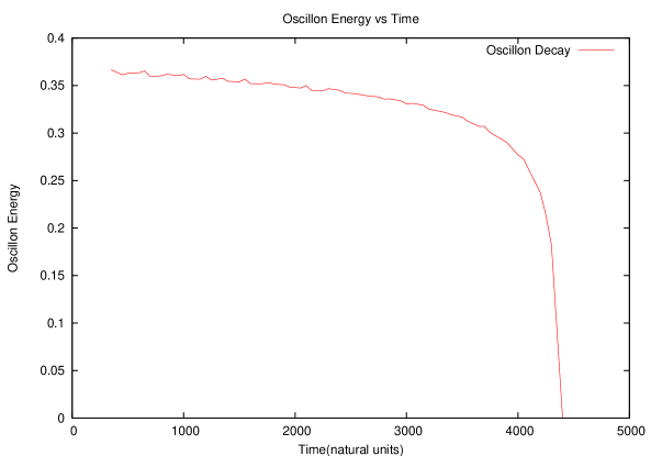
Figure 1: The final decay of an oscillon as it approaches the point of instability. Although the decay is very sudden, the approach to this decay at earlier times is extremely gradual. Here the energy is measured in units of $m$ and the time is measured in units of $1/m$.

The dramatic behavior shown in Fig. 1 is visible only at the end of the oscillon’s life, however. For slightly higher energies, this curve becomes extremely close to horizontal; oscillons with only marginally higher energy lie far to the left. As a result, the oscillon lifetime scales exponentially with its energy, as shown in Fig. 2. Here we have used the energy to select oscillons that we predict will decay in a reasonable amount of time. However, we have also verified that more energetic oscillons live for the exponentially long times that this analysis would suggest. In particular, we have followed an individual oscillon for times exceeding $2\times 10^{7}$ in natural units. This analysis also verifies that the decay is not the result of accumulated numerical error.

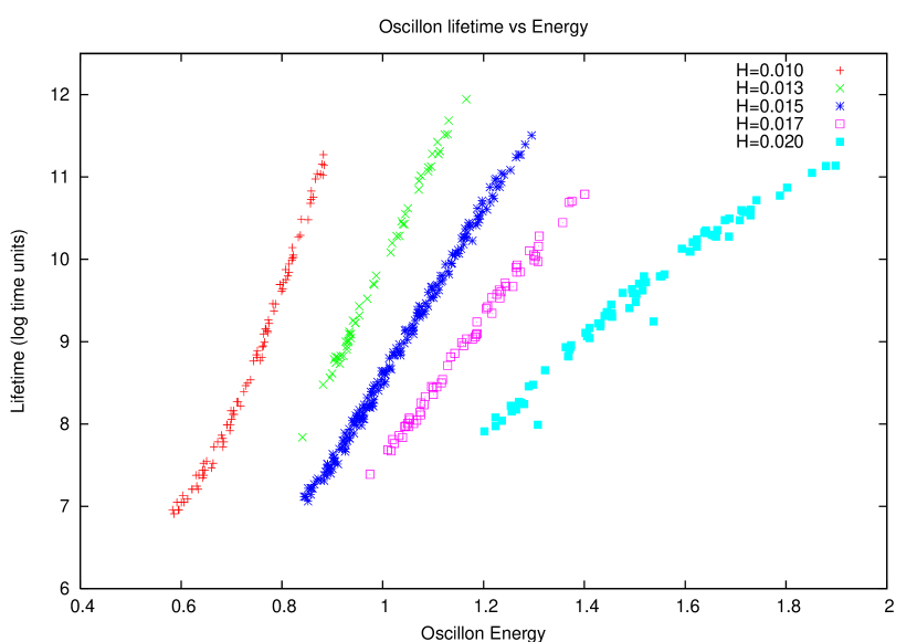
Figure 2: Logarithmic plot of oscillon lifetime as function of the initial oscillon energy for various values of the Hubble constant $H$. The vertical axis is the natural logarithm of the lifetime of the oscillon and the horizontal axis is the oscillon energy, both in units where $m=1$. We see that the oscillon lifetime scales like $\exp(kE/m)/m$, where $E$ is the oscillon energy. The rate of exponential growth $k$ is given in as a function of $H$ in the table at right. The values of $k$ are roughly linear in $H$, with a slope of approximately $-994/m$.

$H/m$	$k$
0.010	14.7
0.013	12.9
0.015	10.2
0.017	8.35
0.020	4.97

To track the flow of energy during the oscillon’s decay, we consider a fiducial box with a radius of one Hubble length $1/H$. The rate of change in the energy within the box is then

$$\frac{dE_{\rm box}}{dt} = \left.\frac{\dot{\phi}\phi^{\prime}}{a(t)}\right|_{-1/H}^{1/H}-\int_{-1/H}^{1/H}p\,\dot{a}(t)dx$$ (16)

where the first term represents the flow of of any outgoing waves through the boundary and the second represents the energy lost to gravitational expansion. For our oscillon configurations, both terms oscillate. On average, however, we find the surprising result that the first term is both positive and much smaller in magnitude than the second term, meaning that the oscillon decays due to energy lost through the expansion rather than through the emission of scalar field waves.

Finally, we note that although the expansion of the universe explicitly introduces an exponentially large scale — the size of the universe — it is irrelevant to the oscillon lifetime. The oscillon only sees its local region of space, which is expanding at a rate of order one in natural units, with greater expansion of the universe corresponding to shorter oscillon lifetimes.

V Conclusions

We have found that oscillon lifetimes in an expanding background scale exponentially with the oscillon’s energy in a simple toy model. The oscillon configurations form generically from an uncorrelated thermal background. As a result, although all the parameters of our theory are of order one in natural units, the dynamics of the theory generates an exponentially large time scale through the oscillon’s decay. Although our analysis is limited to one dimension, we have also conducted preliminary experiments showing similar behavior when the three-dimensional oscillons of Refs. Gleiser ; oscillon are coupled to an expanding background in an ansatz with spherical symmetry. Work is in progress group to explore the possible consequences of these ideas in the early universe.

VI Acknowledgments

We thank N. Alidoust, E. Farhi, A. H. Guth, A. Scardicchio, R. Rosales, and R. Stowell for assistance. We also thank J. Dunham and M. Gleiser for discussions. N. G. and N. S. were supported in part by Research Corporation through a Cottrell College Science Award. N. G. was also supported in part by the National Science Foundation through the Vermont Experimental Program to Stimulate Competitive Research (VT-EPSCoR) and the Middlebury Faculty Professional Development Fund. N. S. was also supported in part by the Middlebury Undergraduate Collaborative Research Fund.

References

- (1) R. F. Dashen, B. Hasslacher, and A. Neveu, Phys. Rev. D11 (1975) 3424.
- (2) S. Coleman, Nucl. Phys. B262 (1985) 263.
- (3) D. K. Campbell, J. F. Schonfeld and C. A. Wingate, Physica 9D, 1 (1983).
- (4) I. L. Bogolubsky and V. G. Makhankov, JETP Lett 24 (1976) 12.
- (5) M. Gleiser, hep-ph/9308279, Phys. Rev. D49 (1994) 2978; E. J. Copeland, M. Gleiser and H. R. Muller, hep-ph/9503217, Phys. Rev. D52 (1995) 1920; A. Adib, M. Gleiser, and C. Almeida, hep-th/0203072, Phys. Rev. D66 (2002) 085011.
- (6) E. P. Honda and M. W. Choptuik, hep-ph/0110065, Phys. Rev. D65 (2002) 084037.
- (7) S. Kasuya, M. Kawasaki, and F. Takahashi, hep-ph/0209358, Phys. Lett. B559 (2003) 99.
- (8) B. Piette and W. J. Zakrzewski, Nonlinearity 11 (1998) 1103.
- (9) C. Rebbi and R. Singleton, Jr., hep-ph/9601260, Phys. Rev. D54 (1996) 1020; P. Arnold and L. McLerran, Phys. Rev. D37 (1988) 1020;
- (10) G. Fodor and I. Racz, hep-th/0311061, Phys. Rev. Lett. 92 (2004) 151801; P. Forgacs and M. S. Volkov, hep-th/0311062, Phys. Rev. Lett. 92 (2004) 151802.
- (11) E. Farhi, N. Graham, V. Khemani, R. Markov, and R. R. Rosales, hep-th/0505273, Phys. Rev. D72 (2005) 101701.
- (12) H. Segur and M. D. Kruskal, Phys. Rev. Lett. 58 (1987) 747.
- (13) N. Alidoust, E. Farhi, N. Graham, A. H. Guth, K. Pathak, N. Stamatopoulos, R. R. Rosales, J. Shelton, and R. Stowell, work in progress.
- (14) M. Broadhead and J. McDonald, hep-ph/0503081, Phys. Rev. D72 (2005) 043519.
- (15) M. Gleiser, hep-th/0602187.
- (16) E. Kolb and I. Tkachev, astro-ph/9311037, Phys. Rev. D49 (1994) 5040.
- (17) J. Smit, hep-lat/0510106, PoS LAT2005 (2005) 022.
- (18) M. Gleiser and A. Sornborger, patt-sol/9909002, Phys. Rev. E62 (2000) 1368.
- (19) M. Gleiser and R. C. Howell, hep-ph/0209176, Phys. Rev. E68 (2003) 065203(R); M. Gleiser and R. C. Howell, hep-ph/0409179, Phys. Rev. Lett. 94 (2005) 151601. M. Gleiser, hep-th/0602187.
- (20) A. M. Kosevich and A. S. Kovalev, Zh. Eksp. Teor. Fiz. 67 (1975) 1793 [Sov. Phys. JETP 40 (1975) 891]; R. R. Rosales, “Weakly Nonlinear Expansions for Breathers,” unpublished research notes; J. N. Hormuzdiar and S. D. Hsu, Phys. Rev. C59 (1999) 889.