Supermassive screwed cosmic string in dilaton gravity

Abstract

The early Universe might have undergone phase transitions at energy scales much higher than the one corresponding to the Grand Unified Theories (GUT) scales. At these higher energy scales, the transition at which gravity separated from all other interactions; the so-called Planck era, more massive strings called supermassive cosmic strings, could have been produced, with energy of about $10^{19}GeV$. The dynamics of strings formed with this energy scale cannot be described by means of the weak-field approximation, as in the standard procedure for ordinary GUT cosmic strings. As suggested by string theories, at this extreme energies, gravity may be transmitted by some kind of scalar field (usually called the dilaton) in addition to the tensor field of Einstein’s theory of gravity. It is then permissible to tackle the issue regarding the dynamics of supermassive cosmic strings within this framework. With this aim we obtain the gravitational field of a supermassive screwed cosmic string in a scalar-tensor theory of gravity. We show that for the supermassive configuration exact solutions of scalar-tensor screwed cosmic strings can be found in connection with the Bogomol’nyi limit. We show that the generalization of Bogomol’nyi arguments to the Brans-Dicke theory is possible when torsion is present and we obtain an exact solution in this supermassive regime, with the dilaton solution obtained by consistency with internal constraints.

1 Introduction

Topological defects such as cosmic strings[1, 2] are predicted to form in the early Universe, at GUT scale, as a result of symmetry-breaking phase transitions envisaged in gauge theories of elementary particles interactions. These topological defects may also help to explain the most energetic events in the Universe, as the cosmological Gamma-Ray Bursts (GRBs)[3], very high energy neutrinos[4] and gravitational-wave bursts[5].

Cosmic strings can also be formed by phase transitions at energy scales higher than the GUT scale, which result in the production of more massive strings. The current theory tells us that these strings had been produced before or during inflation, so that their dynamical effects would not leave any imprints in the Cosmic Microwave Background radiation(CMB). These cosmic strings are referred to as supermassive cosmic strings and had an energy of approximately three orders of magnitude higher than the ordinary cosmic string. This means that they can no longer be treated by using the weak-field approximation.

The space-time of supermassive cosmic strings has been examined by Laguna and Garfinkle[6] following a method developed by Gott[7]. Their approach considered carefully the possible asymptotic behavior of the supermassive cosmic string metric. Their conclusions were that such a string has a Kasner-type metric outside the core with an internal metric that is regular.

Some authors have studied solutions corresponding to topological defects in different contexts like in Brans-Dicke [8], dilaton theory [9], and in more general scalar-tensor couplings [10, 11]. In this paper we study, within the framework of a scalar-tensor theory of gravity, the dynamics of matter in the presence of a supermassive screwed cosmic string (SMSCS) that had been produced in the very early Universe.

Scalar-tensor theories of gravity can be considered[12] as the most promising alternatives for the generalization of Einstein’s gravity, and is motivated by string theory. In scalar-tensor theories, gravity is mediated by a long-range scalar field in addition to the usual tensor field present in Einstein’s theory [12]. Scalar-tensor theories of gravity are currently of particular interest since such theories appear as the low energy limit of supergravity theories constructed from string theories[13] and other higher dimensional gravity theories[14]. However, due to the lack of a full non-perturbative formulation, which allows a description of the early Universe close to the Planck time, it is necessary to study classical cosmology prior to the GUT epoch by recurring to the low-energy effective action induced by string theory. The implications of such actions for the process of structure formation have been studied recently[11, 15].

This work is outlined as follows. In Section 2, we describe the configuration of a supermassive screwed cosmic string (SMSCS) in scalar-tensor theory of gravity. In Section 3, we construct the Bogomol’nyi conditions of a screwed cosmic string in scalar-tensor theory. In Section 4, we solve the exact equations for the exterior spacetime, by applying Linet’s method[16]. Then, we match the exterior solution to the internal one. We also derive the deficit angle associated with the metric of a SMSCS. Section 5 discusses the particle motion around this kind of defect. In Section 6, our discussion and conclusions are presented.

2 Cosmic string in dilaton-torsion gravity

The scalar-tensor theory of gravity with torsion can be described by the action which is given (in the Jordan-Fierz frame) by

$${\cal S}=\frac{1}{16\pi}\int d^{4}x\sqrt{-\tilde{g}}\left[\tilde{\Phi}\tilde{R}-\frac{\omega(\tilde{\Phi})}{\tilde{\Phi}}\tilde{g}^{\mu\nu}\partial_{\mu}\tilde{\Phi}\partial_{\nu}\tilde{\Phi}\right]+{\cal S}_{m}[\Psi_{m},\tilde{g}_{\mu\nu}],$$ (1)

where ${\cal S}_{m}$ is the action of all matter fields and $\tilde{g}_{\mu\nu}$ is the metric in the Jordan-Fierz frame. In this frame, the Riemann curvature scalar, $\tilde{R}(\{\})$, can be written as

$$\tilde{R}=\tilde{R}(\{\})+\epsilon\frac{\partial_{\mu}\tilde{\Phi}\partial^{\mu}\tilde{\Phi}}{\tilde{\Phi}^{2}}\;,$$ (2)

with $\epsilon$ being the torsion coupling constant [11]. Note that in this theory matter couples minimally and universally with $\tilde{g}_{\mu\nu}$ and not with $\tilde{\Phi}$.

For technical reasons, working in the Einstein or conformal frame is more simple. In this frame, the kinematic terms associated with the scalar and tensor fields do not mix and the action is given by

$${\cal S}=\frac{1}{16\pi G}\int d^{4}x\sqrt{-g}\left[R(\{\})-2\kappa(\phi)g^{\mu\nu}\partial_{\mu}\phi\partial_{\nu}\phi\right]+{\cal S}_{m}[\Psi_{m},\Omega^{2}(\phi)g_{\mu\nu}],$$ (3)

where $g_{\mu\nu}$ is a pure rank-2 tensor in the Einstein frame and $\Omega(\phi)$ is an arbitrary function of the scalar field.

Action (3) is obtained from (1) by a conformal transformation

$$\tilde{g}_{\mu\nu}=\Omega^{2}(\phi)g_{\mu\nu},$$ (4)

and by a redefinition of the quantity

$$G\Omega^{2}(\phi)=\tilde{\Phi}^{-1}\;,$$ (5)

which makes evident that any gravitational phenomena will be affected by the variation of the gravitation “constant” $G$ in scalar-tensor theories of gravity. Let us introduce a new parameter, $\alpha$, such that

$$\alpha^{2}\equiv\left(\frac{\partial\ln\Omega(\phi)}{\partial\phi}\right)^{2}=[2\omega(\tilde{\Phi})+3]^{-1},$$ (6)

which can be interpreted as the (field-dependent) coupling strength between matter and the scalar field. In order to make our calculations as general as possible, we will not specify the factors $\Omega(\phi)$ and $\alpha(\phi)$, thus leaving them as arbitrary functions of the scalar field.

In the conformal frame, the Einstein equations read as

$$G_{\mu\nu}=2\kappa\partial_{\mu}\phi\partial_{\nu}\phi-\kappa g_{\mu\nu}g^{\alpha\beta}\partial_{\alpha}\phi\partial_{\beta}\phi+8\pi GT_{\mu\nu}\;.$$ (7)

where $\kappa$ is a function defined by

$$\kappa=1-2\epsilon\alpha(\phi)^{2}\;,$$ (8)

which explicitly depends on the scalar field and torsion. The energy-momentum tensor is defined as

$$T_{\mu\nu}\equiv\frac{2}{\sqrt{-g}}\frac{\delta{\cal S}_{m}}{\delta g_{\mu\nu}},$$ (9)

which is no longer conserved. It is clear from (4) that we can relate the energy-momentum tensor in both frames in such a way that

$$\tilde{T}^{\mu}_{\nu}=\Omega^{-4}(\phi)T^{\mu}_{\nu}\;.$$ (10)

For the sake of simplicity, in what follows we will focus on the Brans-Dicke theory where $\Omega^{2}(\phi)=e^{2\alpha\phi}$. To account for the (unknown) coupling of the cosmic string field with the dilaton, we will choose the action, $\cal S$, in the Einstein frame, as

$${\cal S}=\frac{1}{16\pi G}\int d^{4}x\sqrt{-g}\left[R-2g^{\mu\nu}\kappa\partial_{\mu}\phi\partial_{\nu}\phi+e^{2(a+2)\alpha\phi}{\cal L}_{m}[\psi_{m},e^{2\alpha\phi}g_{\mu\nu}]\right]\;,$$ (11)

where $a$ is an arbitrary parameter which couples the dilaton to the matter fields.

Taking into consideration the symmetry of the source, we impose that the metric is static and cylindrically symmetric. Thus, let us choose a general cylindrically symmetric metric with coordinates $(t,\rho,z,\theta)$ as

$$ds^{2}=e^{\gamma}(-dt^{2}+d\rho^{2}+dz^{2})+\beta^{2}e^{-\gamma}d\theta^{2},$$ (12)

where the metric functions $\gamma$ and $\beta$ are functions of the radial coordinate $\rho$ only. In addition, the metric functions satisfy the regularity conditions at the axis of symmetry ($\rho=0$)

$$\gamma=0,\;\;\frac{d\gamma}{d\rho}=0\;\;\mbox{and}\;\;\frac{d\beta}{d\rho}=1.$$ (13)

Next we will search for a regular solution of a self-gravitating vortex in the framework of a scalar-tensor gravity. Hence, the simplest bosonic vortex arises from the Lagrangean of the Abelian-Higgs $U(1)$ model, which contains a complex scalar field plus a gauge field and can be written as

$${\cal L}_{m}=-\frac{1}{2}\tilde{g}^{\mu\nu}D_{\mu}\varphi D_{\nu}\varphi^{*}-\frac{1}{4}\tilde{g}^{\mu\nu}\tilde{g}^{\alpha\beta}F_{\mu\alpha}F_{\nu\beta}-V(\mid\varphi\mid)$$ (14)

where $D_{\mu}\varphi\equiv(\partial_{\mu}+ieA_{\mu})\varphi$ and $F_{\mu\nu}$ is the field-strength associated with the vortex $A_{\mu}$. The potential is ”Higgs-inspired” and contains appropriate $\varphi$ interactions so that there occurs a spontaneous symmetry breaking. It is given by

$$V(\mid\varphi\mid)=\frac{\lambda_{\varphi}}{4}(\mid\varphi\mid^{2}-\eta^{2})^{2},$$ (15)

with $\eta$ and $\lambda_{\phi}$ being positive parameters. A vortex configuration arises when the $U(1)$ symmetry associated with the $(\varphi,A_{\mu})$ pair is spontaneously broken in the core of the vortex. In what follows, we will restrict ourselves to configurations corresponding to an isolated and static vortex along the $z$-axis. In a cylindrical coordinate system $(t,\rho,\theta,z)$, such that $\rho\geq 0$ and $0\leq\theta<2\pi$, we make the choice

$$\varphi=R(\rho)e^{i\theta}\;\;\mbox{and}\;\;A_{\mu}=\frac{1}{q}[P(\rho)-1]\delta^{\theta}_{\mu},$$ (16)

in analogy with the case of ordinary (non-conducting) cosmic strings. The variables $R,P$ are functions of $\rho$ only. We also require that these functions are regular everywhere and so they must satisfy the usual boundary conditions for a vortex configuration[17], which are the following

$$R(0)=0\;\;\mbox{and}\;\;P(0)=1$$

$$\lim_{\rho\rightarrow\infty}R(\rho)=\eta\;\;\mbox{and}\lim_{\rho\rightarrow\infty}P(\rho)=0.$$ (17)

With the metric given by Eq.(12) we are in a position to write down the full equations of motion for the self-gravitating vortex in a scalar-tensor gravity. In the conformal frame these equations reduce to

$$\beta^{{}^{\prime\prime}} = 8\pi G\beta[T^{t}_{t}+T^{\rho}_{\rho}]e^{\gamma}$$ (18)

$$(\beta\gamma^{\prime})^{\prime} = 8\pi G\beta[T^{\rho}_{\rho}+T^{\theta}_{\theta}]e^{\gamma},$$ (19)

$$\beta^{{}^{\prime}}\gamma^{{}^{\prime}} = \frac{\beta(\gamma^{{}^{\prime}})^{2}}{4}-\kappa\beta(\phi^{{}^{\prime}})^{2}+8\pi Ge^{\gamma}T^{\rho}_{\rho}$$ (20)

$$(\kappa\beta\phi^{{}^{\prime}})^{{}^{\prime}} = -4\pi G\alpha\beta\left[(a+1)T^{t}_{t}+T^{\rho}_{\rho}+T^{\theta}_{\theta}\right]e^{\gamma},$$ (21)

where $(^{\prime})$ denotes derivative with respect to $\rho$.

In what follows we will analyze the Bogomonl’nyi conditions for this supermassive cosmic string in this dilaton-torsion theory. In some models [18, 19], it is possible to work with first order differential equations, which are called Bogomol’nyi equations, instead of more complicated Euler-Lagrange equations. This approach can be applied to Eqs.(18-21) when $\kappa=0$ and $a=-1$. The traditional method to obtain such equations [18, 19] is based on rewriting an expression for the energy of a field configuration, in such a way that it has a lower bound, which is of topological origin. The field configurations which saturate this bound satisfy Euler-Lagrange equations as well as Bogomol’nyi equations.

3 Bogomol’nyi bounds for dilatonic supermassive cosmic strings

The gravitational field produced by a supermassive cosmic string in the framework of general relativity has been studied by numerical method [6] in the case $G\mu=1/4$, where $\mu$ is the linear mass density of the string, in the Bogomonl’nyi limit. In this case, the exact field equations lead to the metric of a cylindrical spacetime [19, 20, 21]. In this section, we analyse the possibility of finding a Bogomol^′nyi bound for a dilatonic-torsion cosmic string. It is worth commenting that in the usual Brans-Dicke theory this limit is not possible[9], but in the space-time with torsion it is possible. In this case the dilaton does not have any dynamics, that is, $\kappa=0$, but even in this situation the solution is non-trivial. As the Bogomonl’nyi equations are differential equations of first order, as a consequence in the supermassive screwed cosmic string case we can find an exact solution. In order to do this we have to compute the energy-momentum tensor which can be written as

$$T^{\mu}_{\nu}=2g^{\mu\alpha}\frac{\partial{\cal L}}{\partial g^{\alpha\nu}}-\delta^{\mu}_{\nu}{\cal L},$$ (22)

whose non-vanishing components are

$$T^{t}_{t}=T^{z}_{z}=-\frac{1}{2}e^{2(a+1)\alpha\phi}\{e^{-\gamma}R^{\prime 2}+\frac{e^{\gamma}}{\beta^{2}}R^{2}P^{2}+\frac{e^{-2\alpha\phi}}{\beta^{2}}(\frac{P^{\prime 2}}{4\pi q^{2}})+2e^{2\alpha\phi}V(R)\}\;,$$ (23)

Note that from (23) we see that the boost symmetry is not preserved. This fact is related with the absence of current in $z$-direction, as in the usual ordinary cosmic string.

The transverse components of the energy-momentum tensor are given by the expressions

$$T^{\rho}_{\rho}=\frac{1}{2}e^{2(a+1)\alpha\phi}\{e^{-\gamma}R^{\prime 2}-\frac{e^{\gamma}}{\beta^{2}}R^{2}P^{2}+\frac{e^{-2\alpha\phi}}{\beta^{2}}(\frac{P^{\prime 2}}{4\pi q^{2}})-2e^{2\alpha\phi}V(R)\}\;,$$ (24)

$$T^{\theta}_{\theta}=-\frac{1}{2}e^{2(a+1)\alpha\phi}\{e^{-\gamma}R^{\prime 2}-\frac{e^{\gamma}}{\beta^{2}}R^{2}P^{2}-\frac{e^{-2\alpha\phi}}{\beta^{2}}(\frac{P^{\prime 2}}{4\pi q^{2}})+2e^{2\alpha\phi}(\phi)V(R)\}\;.$$ (25)

As stated earlier, the energy-momentum tensor is not conserved in the conformal frame. Thus, in this situation, we have

$$\nabla_{\mu}T^{\mu}_{\nu}=\alpha(\phi)T\nabla_{\nu}\phi,$$

where $T$ is the trace of the energy-momentum tensor. This equation gives an additional relation between the scalar field $\phi$ and the source described by $T^{\mu}_{\nu}$. This energy-momentum tensor has only an $\rho$-dependence. The matter field equations can be written as

$$R^{\prime\prime}+R^{\prime}\left[\frac{\beta^{\prime}}{\beta}-2(a+1)\alpha\phi^{\prime}\right]-R\left[\frac{P^{2}}{\beta^{2}}+4\lambda e^{2\alpha\phi}(R^{2}-\eta^{2})\right]=0\;,$$ (26)

$$P^{\prime\prime}+P^{\prime}\left[\frac{\beta^{\prime}}{\beta}-2(a+2)\alpha\phi^{\prime}\right]-q^{2}R^{2}Pe^{2\alpha\phi}=0\;.$$ (27)

Now let us define the energy density per unit of length of the string (in Jordan-Fierz frame), $\mu$, as

$$\mu=2\pi\int_{0}^{\infty}\sqrt{-\tilde{g}}\tilde{T}_{t}^{t}d\rho\;.$$ (28)

Considering the $t$-component of the energy-momentum tensor given by (23) we realize that $a=-1$ is a rather special point in the analysis of the Bogomol’nyi solution. Following the studies in the literature [9, 16] we analyzed the case where $\gamma=0$. In such a situation it is possible to find the Bogomonl’nyi solution for $\kappa=0$ because this is the only value of this parameter that turns equation (20) consistent with the fact that the transverse component of energy-momentum tensor vanishes. Considering the Einstein frame and the expression for $T^{t}_{t}$ given by Eq.(23), Eq.(28) turns into

$$\begin{array}[]{ll}\mu=&2\pi\int_{0}^{\infty}\beta d\rho\left[\frac{1}{2}\left(\frac{P^{\prime}}{q\beta}e^{-\alpha\phi}+e^{\alpha\phi}\sqrt{2\lambda}(R^{2}-\eta^{2})\right)^{2}+\frac{1}{q\beta}\sqrt{2\lambda}(R^{2}-\eta^{2})P^{\prime}+\right.\\ &\left.+\left(R^{\prime}+\frac{RP}{\beta}\right)^{2}-\frac{2}{\beta}e^{2\alpha\phi}RPR^{\prime}\right],\end{array}$$ (29)

where we have taken into account relations between $\tilde{T}_{\nu}^{\mu}$ and $T_{\nu}^{\mu}$ and$\tilde{g}_{\mu\nu}$ and $g_{\mu\nu}$, given by Eqs. (4) and (10), respectively. Using the Bogomonl’nyi method we have that the quadratic terms in (29) vanish and therefore we get

$$\mu=2\pi\int_{0}^{\infty}\beta d\rho\left[\frac{1}{q\beta}\sqrt{2\lambda}(R^{2}-\eta^{2})P^{\prime}-\frac{2}{\beta}e^{2\alpha\phi}RPR^{\prime}\right].$$ (30)

Let us analyze the behavior of the dilaton field and the supermassive cosmic string limit. To do this, let us write

$$\mu=\pi\int_{0}^{\infty}[(R^{2}-\eta^{2})P]^{\prime}\;d\rho$$ (31)

where the Bogomol’nyi limit, $8\lambda=q^{2}$, was taken into account. Integrating by parts and using the regularity conditions (13) and the boundary conditions (17), we find

$$\mu\geq\pi\eta^{2}\;,$$ (32)

with $\mu=\pi\eta^{2}$ being the lower bound which corresponds to a solution in the Bogomol^′nyi limit. We can see that there is no force between vortices and also that the equations of motion are of first order. The search of the Bogomol^′nyi bound for the energy, in the Bogomol^′nyi limit, yields the following system of equations

$$R^{\prime}=-\frac{RP}{\beta}\;,$$ (33)

$$P^{\prime}=-\frac{q^{2}}{2}\beta e^{2\alpha\phi}(R^{2}-\eta^{2})\;.$$ (34)

¿From these equations one can see that the transversal components of the energy-momentum tensor density vanish, that is, $T^{\rho}_{\rho}=T^{\theta}_{\theta}=0$, while the non-zero components $T^{t}_{t}$ and $T^{z}_{z}$, are related by $T^{t}_{t}=T^{z}_{z}$. This corresponds to the minimal configuration asociated with a cosmic string in scalar-tensor theories of gravity.

In the ordinary case, with no torsion, this configuration is not allowed because $\epsilon=0$ and as a consequence there is no possibility to obtain the Bogomonl’nyi configuration with $\phi\neq 0$. Then, the presence of the torsion is of fundamental importance to obtain the Bogomonl’nyi bound in the framework of scalar-tensor theories.

With these conditions one can simplify Eq.(18), which results in

$$\beta^{\prime\prime}=-8\pi G[\frac{R^{2}P^{2}}{\beta}+\frac{q^{2}}{4}\beta(R^{2}-\eta^{2})^{2}e^{2\alpha\phi}]\;.$$ (35)

Using Eqs.(33), (34) in (35) we find

$$\beta^{\prime\prime}=8\pi G\left[RPR^{\prime}+\frac{1}{2}(R^{2}-\eta^{2})P^{\prime}\right]\;,$$ (36)

which has the usual form obtained in the context of general relativity. One can also see that the dilaton only appears in Eq.(34). Then, it is possible to evaluate the integral of Eq.(36), which gives us

$$\beta^{\prime}=-4\pi G(R^{2}-\eta^{2})P+1-4\pi G\eta^{2}\;.$$ (37)

In this section we have analyzed the conditions to obtain the Bogomonl’nyi the bounds for a SMSCS. We note that for $a=-1$ with $\kappa=0$ it is possible that this topological bound can be saturated. In this case, we can see from Eq.(8) that the scalar-tensor parameter $\alpha$ is connected with the torsion through the relation $\alpha^{2}=\frac{1}{2\epsilon}$. In fact, in the Einstein frame, Eq.(7) does not give us the contribution from the dilaton-torsion term. The modification introduced in this limit, that could have occurred in the early Universe, appears in Eq.(34). The $\phi$-solution can be valuable in connection with the cosmic string fields. In the next section, we will attempt to solve the field equations (33), (34) and (37) in the limit of the supermassive screwed cosmic string. For this purpose we divide the space-time in two regions: an exterior region $\rho>\rho_{0}$ and an interior region $\rho\leq\rho_{0}$, where all the string fields contribute to the energy-momentum tensor. Once these separate solutions are obtained, we then match them providing a relationship between the internal parameters of the string and the space-time geometry outside it.

4 Supermassive limit of dilatonic cosmic strings

Now, let us analyze the possibility of obtaining an exact solution of the first-order differential equations studied in the last section. It is possible to find the supermassive limit of a $U(1)$ gauge cosmic string in scalar-tensor theories of gravity with torsion. Using the transformations [22]

$$\begin{array}[]{ll}\beta=\frac{2\sqrt{2}}{\eta q}\bar{\beta}\;,\\ R=\eta\bar{R}\;,\\ \rho=\frac{2\sqrt{2}}{\eta q}\bar{\rho}\;,\end{array}$$ (38)

and the relation $\bar{\eta}^{2}=4\pi G\eta^{2}$, we obtain the equations of the motion in the supermassive limit $\bar{\eta}^{2}=1$. They are given by

$$\bar{\beta}^{\prime}=-\bar{P}(\bar{R}^{2}-1)\;,$$ (39)

$$\bar{P}^{\prime}=4\bar{\beta}(\bar{R}^{2}-1)e^{2\alpha\phi}\;,$$ (40)

$$\bar{R}^{\prime}=\frac{\bar{R}\bar{P}}{\bar{\beta}}\;.$$ (41)

Now, we consider the solutions of these equations in two regions: the internal, where $\bar{R}^{2}<<1$, and the external one. As stressed earlier, we do not use the weak field approximation to derive this internal solution because at the energy scale of the transition which allows the formation of such supermassive comsic string, such an approach cannot be applied.

4.1 Internal exact solution

To solve these equations we make the assumption that $\bar{R}^{2}<<1$, if we consider that the radius of the string is of the order of $10^{-30}cm$. Thus, the interior solution of the field equations, in the first order approximation in $\bar{R}$, may be taken as

$$\bar{\beta}^{\prime}=\bar{P}\;,$$ (42)

$$\bar{P}^{\prime}=-4\bar{\beta}e^{2\alpha\phi}\;,$$ (43)

$$\bar{R}^{\prime}=\frac{\bar{R}\bar{P}}{\bar{\beta}}\;.$$ (44)

The solution then reads

$$\bar{\beta}=(1+m)^{-1}\left[m\bar{\rho}+\frac{1}{2}\sin(2\bar{\rho})\right]\;,$$ (45)

$$\bar{P}=(1+m)^{-1}[m+\cos(2\bar{\rho})]\;,$$ (46)

where $m$ is a constant.

Now, let us consider the solution for the field $\bar{R}$ taking into account Eq.(44). Thus, we have

$$\bar{R}=B(1+m)^{-1}\left[m\bar{\rho}+\frac{1}{2}\sin(2\bar{\rho})\right]\;,$$ (47)

with $B=(1+m)^{-1}\left[m\bar{\rho}_{0}+\frac{1}{2}\sin(2\bar{\rho}_{0})\right]$, in such a way that at the boundary $\bar{\rho}=\bar{\rho}_{0}$, $\bar{R}(\bar{\rho}_{0})=1$. The dilaton solution thus reads

$$\phi=\frac{1}{2\alpha}\ln\left\{\frac{\sin(\sqrt{\frac{\lambda}{\pi}}{\rho})}{[m\sqrt{\frac{\lambda}{\pi}}{\rho}+\sin(\sqrt{\frac{\lambda}{\pi}}{\rho})]}\right\}\;,$$ (48)

with ${\rho}=\sqrt{x^{2}+y^{2}}$ and the $\phi$ solution given in Fig.1.

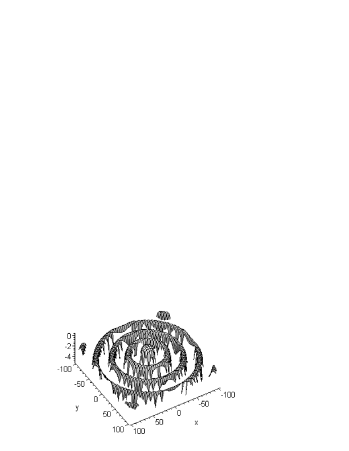
Figure 1: The $\phi$ solution as a function of x and y for $m=0.2$,   $\sqrt{\frac{\lambda}{\pi}}=0.2$ and $\alpha=0.5$, with x and y in the range     $-100\leq x\leq 100$ and $-100\leq y\leq 100$.

The Fig. 1 shows the exact solution for a supermassive screwed cosmic string when the limit $\bar{R}<<1$ is applicable.

4.2 External solution and the matched conditions

Now we will analyze the assymptotic solution for $\rho\geq\rho_{0}$ and apply the boundary and matching conditions. To do this we have to obtain the exterior solution. As this solution corresponds to the exterior region, thus we consider $T^{\mu}_{\nu}=0$. For this region, the metric in the Einstein frame takes the form

$$ds^{2}=-dt^{2}+d{\rho}^{2}+dz^{2}+\beta_{\infty}^{2}d\theta^{2}\;,$$ (49)

in an appropriate coordinate system where the constant $\beta_{\infty}$ fixes the radius of the compactified dimension. This asymptotic form of the metric given by Eq.(49) for a cosmic string has been already examined in literature [20]. In the case of a space-time with torsion, we can find the matching conditions using the fact that$[\{^{\alpha}_{\mu\nu}\}]_{{}_{{\rho}={\rho}_{0}}}^{(+)}=[\{^{\alpha}_{\mu\nu}\}]_{{}_{{\rho}={\rho}_{0}}}^{(-)}$, and the metricity constraint $[g_{\mu\nu}K_{(\mu\nu)}^{\hskip 8.5359pt\alpha}]_{{}_{{\rho}={\rho}_{0}}}^{+}=[g_{\mu\nu}K_{(\mu\nu)}^{\hskip 8.5359pt\alpha}]_{{}_{{\rho}={\rho}_{0}}}^{-}$, for the contorsion. Thus, we find the following continuity conditions

$$[g_{\mu\nu}]_{{}_{{\rho}={\rho}_{0}}}^{(-)}=[g_{\mu\nu}]_{{}_{{\rho}={\rho}_{0}}}^{(+)},$$

$$[\frac{\partial g_{\mu\nu}}{\partial x^{\alpha}}]_{{}_{{\rho}={\rho}_{0}}}^{(+)}=[\frac{\partial g_{\mu\nu}}{\partial x^{\alpha}}]_{{}_{{\rho}={\rho}_{0}}}^{(-)},$$ (50)

where $(-)$ represents the internal region and $(+)$ corresponds to the external region around ${\rho}={\rho}_{0}$[23, 24]. For a supermassive U(1) gauge cosmic string in the Bogomonl’ny limit where $q^{2}=8\lambda$ and $\mu=\pi\eta^{2}$, thus we find that

$$\frac{2\sqrt{2}}{\eta q}\frac{1}{1+m}\left[m\bar{\rho}_{0}+\frac{1}{2}\sin(2\bar{\rho}_{0})\right]=\beta_{\infty}\;,$$ (51)

and

$$\frac{1}{1+m}\left[m+\cos(2\bar{\rho}_{0})\right]=0\;.$$ (52)

For $\cos 2\bar{\rho}_{0}=-m$ and $\sin 2\bar{\rho}_{0}=\sqrt{1-m^{2}}$, the solution for the long range field $\phi$, in $\bar{\rho}=\bar{\rho}_{0}$, is given by

$$\phi(\bar{\rho}_{0})=\frac{1}{2\alpha}{\bf\ln}\left\{\frac{\sqrt{1-m^{2}}}{[2m\bar{\rho}_{0}+\sqrt{1-m^{2}}]}\right\}\;.$$ (53)

Therefore, the consistent asymptotic solution for the fields in ${\rho}\geq{\rho}_{0}$ are

$$\begin{array}[]{ll}\bar{P}=0,\\ \bar{R}=1\;.\end{array}$$ (54)

This external solution is consistent with the boundary condition given by Eq.(17) for $\bar{\eta}^{2}=1$. Thus, the expression for the linear energy density turns into

$$\mu=\int_{0}^{{\rho}_{0}}\int_{0}^{2\pi}T^{t}_{t}\beta d\theta d{\rho}=\frac{1}{4}\left\{1-(1+m)^{-1}[m+\cos(2\bar{\rho}_{0})]\right\}=\frac{1}{4}\;.$$ (55)

The constant $m$ can be restricted to the range $-1<m<1$. In the Bogomonl’nyi limit, thus the assymptotic form (49) has the coefficient $\beta_{\infty}$ given by

$$\beta_{\infty}=2\sqrt{\frac{\pi}{\lambda}}\frac{1}{1+m}\left[m\bar{\rho}_{0}+\frac{1}{2}\sqrt{1-m^{2}}\right]\;.$$ (56)

One can note that when $m=0$, we have that $\beta_{\infty}=\sqrt{\frac{\pi}{\lambda}}$, and therefore, the contribution arising from the scalar field vanishes, due to the fact that $\phi=0$. In this case we recover the Einstein solution for the supermassive cosmic string[20]. Therefore, the asymptotic metric in the Jordan-Fierz frame is given by

$$ds^{2}=\frac{\sin(\sqrt{\frac{\lambda}{\pi}}{\rho})}{\left[\sqrt{\frac{\lambda}{\pi}}m{\rho}+\sin(\sqrt{\frac{\lambda}{\pi}}{\rho})\right]}\left\{-dt^{2}+d{\rho}^{2}+\beta_{\infty}d\theta^{2}+dz^{2}\right\}\;.$$ (57)

Thus, in the torsion-dilaton case appears a Newtonian force in the Bogomonl’nyi limit of the exact solution. There is no a $\phi$-equation in the supermassive limit, but the $\phi$ solution is found in connection with the internal solution of the field equations for the cosmic string. The continuity in the boundary gives us the $\phi$-exterior solution. It is of the same form as for the interior solution.

5 Particle deflection near a supermassive screwed cosmic string

Now let us consider some new physical effects derived from the obtained solution for a supermassive screwed cosmic string. Thus in order to see these, we study the geodesic equation in the space-time under consideration, given by Eq.(57), where $g_{tt}$ reads

$$g_{tt}=\frac{\sin(\sqrt{\frac{\lambda}{\pi}}{\rho})}{\left[\sqrt{\frac{\lambda}{\pi}}m{\rho}+\sin(\sqrt{\frac{\lambda}{\pi}}{\rho})\right]}\;,$$ (58)

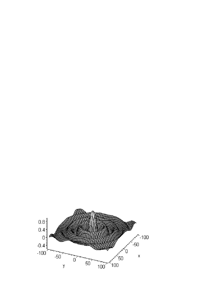
Figure 2: The tt-component of the metric solution as a function of x and y, for $m=0.2$,    $\sqrt{\frac{\lambda}{\pi}}=0.2$ and $\alpha=0.5$, with x and y in the range     $-100\leq x\leq 100$ and $-100\leq y\leq 100$.

whose graph is showed in Fig.(2). We shall consider the effect that torsion plays on the gravitational force generated by a SMSCS on a particle moving around it, by assuming that the particle has no charge. To do this, let us consider the Christoffel symbols in the Jordan-Fierz, $\{^{\mu}_{\alpha\beta}\}_{JF}$, frame as a sum of the contributions arising from the Christoffel symbols in the Einstein frame $\{^{\mu}_{\alpha\beta}\}$, from the contortion given by

$$K_{(\alpha\beta)}^{\hskip 8.5359pt\mu}={\alpha(\phi)\over 2}(\delta^{\mu}_{\alpha}\partial_{\beta}\phi+\delta^{\mu}_{\beta}\partial_{\alpha}\phi-2g_{\alpha\beta}g^{\mu\nu}\partial_{\nu}\phi){\bf\;,}$$ (59)

and from the dilaton field, $\phi$. Thus, summing up these contributions, we have

$$\{^{\mu}_{\alpha\beta}\}_{JF}=\{^{\mu}_{\alpha\beta}\}+K_{(\alpha\beta)}^{\hskip 8.5359pt\mu}+{\alpha(\phi)\over 2}(\delta^{\mu}_{\alpha}\partial_{\beta}\phi+\delta^{\mu}_{\beta}\partial_{\alpha}\phi).$$ (60)

Let us consider the particle moving with speed $|{\bf v}|\equiv dx^{\alpha}/dt\leq 1$, in which case the geodesic equation becomes

$$\frac{d^{2}x^{i}}{dt^{2}}+\{^{i}_{tt}\}_{JF}=0\;,$$ (61)

where $i$ is a spatial coordinate index. In the Einstein frame, the Christoffel symbols are given by

$$\{^{i}_{tt}\}=-{1\over 2}g^{i\rho}\partial^{\rho}h_{tt}={1\over 2}\partial_{\rho}\ln(g_{tt}).$$ (62)

Similarly, for the contortion the nonvanishing part is

$$K^{\hskip 5.69046pt\rho}_{(tt)}=-\frac{\tilde{\phi}^{\prime}}{2\tilde{\phi}}\sim\alpha\phi^{\prime}=\frac{1}{2}\sqrt{\frac{\lambda}{\pi}}m\left[\frac{\sqrt{\frac{\lambda}{\pi}}\rho\cot(\sqrt{\frac{\lambda}{\pi}}\rho)-1]}{\sqrt{\frac{\lambda}{\pi}}m\rho+\sin(\sqrt{\frac{\lambda}{\pi}}\rho)}\right]\;.$$ (63)

We also note that the gravitational pull is related to the $h_{tt}$ component that has an explicit dependence on the torsion, as shown in Eq.(58). From the last equation, the acceleration that the SMSCS exerts on a test particle can be explicitly written as

$$a_{smscs}=-m\sqrt{{\lambda\over\pi}}\frac{\sqrt{{\lambda\over\pi}}\rho\cot\sqrt{\frac{\lambda}{\pi}}\rho-1}{\left[\sqrt{\frac{\lambda}{\pi}}m\rho+\sin\sqrt{\frac{\lambda}{\pi}}\rho\right]}\;.$$ (64)

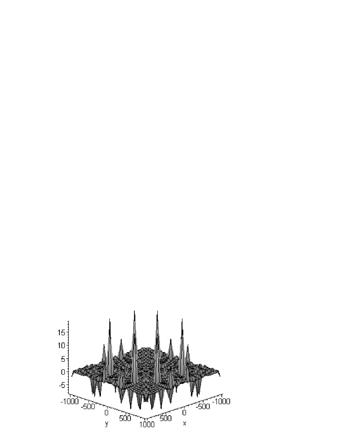
Figure 3: Acceleration as a function of x and y, for $m=0.2$,   $\sqrt{\frac{\lambda}{\pi}}=0.2$ and $\alpha=0.5$, with x and y in the range     $-1000\leq x\leq 1000$ and $-1000\leq y\leq 1000$.

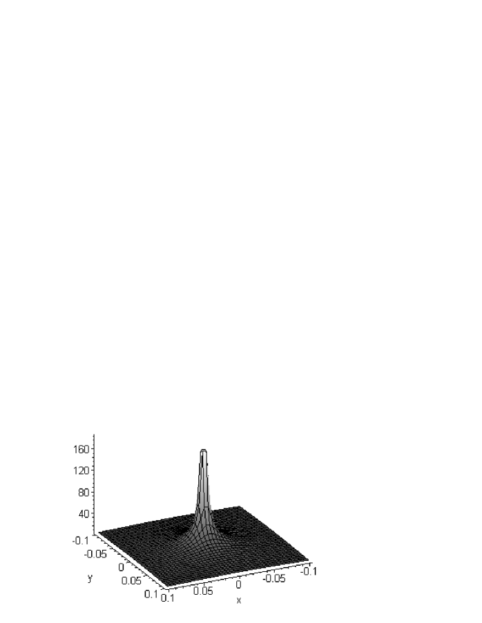
Figure 4: Acceleration as a function of x and y for $m=0.2$,    $\sqrt{\frac{\lambda}{\pi}}=0.2$ and $\alpha=0.5$, with x and y in the range     $-0.1\leq x\leq 0.1$ and $-0.1\leq y\leq 0.1$.

This solution is shown Fig.(3), for a large range. We can also consider the case which corresponds to a region where $\sqrt{\frac{\lambda}{\pi}}\rho$ is very small. In this case, the aceleration can be represented by Fig.(4). By comparing these two graphs one can see that the perturbations introduced by the vortex are perceptible near the string.

A quick glance at the last equation allows us to understand the essential rôle played by torsion in the context of the present formalism. If torsion is present, even in the case in which the string has no current, an attractive gravitational force appears. In the context of the SMSCS, torsion acts in such a way so as to enhance the force that a test particle experiences in the space-time of a SMSCS. Assuming that this string survives inflation and is stable, this enhancement may have meaningful astrophysical and cosmological effects, as for instance, it may in principle influence the process of structure formation in the universe.

6 Conclusion

It is possible that torsion had had a physically relevant role during the early stages of the Universe’s evolution. Along these lines, torsion fields may be potential sources of dynamical stresses which, when coupled to other fundamental fields; for example, the gravitational and scalar fields, might have an important role during the phase transitions leading to the formation of topological defects such as the SMSCS here under consideration. Therefore, it seems stimulating to investigate basic scenarios involving production of topological defects within the context of scalar-tensor theories of gravity with torsion.

It is likely that ordinary cosmic strings could actively perturb the CMB. But these strings cannot be wholly responsible for either the CMB temperature fluctuations or the large scale structure formation of matter. Nonetheless, in the case of supermassive screwed cosmic strings because of the fact that the tension allowed in this situation is much larger than the one corresponding to the ordinary cosmic, and that the torsion, as well as the scalar field, has a non-negligible contribution to the dynamics around the string, one can expect that such a SMSCS can induce perturbations in the universe matter and radiation distribution which are larger than in the case of the ordinary cosmic string. In spite of this, the perturbations by this way driven are certainly not enough to leave significant imprints in the CMB anisotropies as implied by observations.

Thus, from the obtained results we conclude that the torsion as well as the scalar field have a small but non-negligible contribution to the particle dynamics as seen from its modification of the geodesic equation, which is obtained from the contortion term and from the scalar field, respectively. From a physical point of view, these contributions certainly are important and must be considered.

The main motivation to consider this scenario is related to the fact that scalar-tensor gravitational fields are important for a consistent description of gravity, at least at sufficiently high energy scales. Further, the torsion can either induce some physical effects, as the strongest acceleration of particles moving around the string shown above, which could be important at some energy scale, as for example, in the low-energy limit of string theory.

References

- [1] T.W. B. Kibble, J. Phys. A9, 1387 (1976).
- [2] A.Vilenkin, Phys. Rev. D23, 852 (1981); W.A.Hiscock, Phys. Rev. D31, 3288 (1985); D. Garfinkel, Phys. Rev. D32, 1323 (1985).
- [3] R. H. Brandenberger, A. T. Sornborger and M. Trodden, Phys. Rev. D48, 940 (1993); V. Berezinshy, B. Hnatyk and A. Vilenkin, astro-ph/0001213 (2000).
- [4] J. Magueijo and R.H. Brandenberger, astro-ph/0002030, (2000); T.W.B. Kibble, Phys. Rep. 67, 183 (1980).
- [5] T. Damour and A. Vilenkin, Phys. Rev. Lett. 85, 3761 (2000); ibid Phys. Rev. D 64, 064008 (2001); H. J. Mosquera Cuesta and D. Moréjon González, Phys. Lett. B 500, 215 (2001).
- [6] Pablo Laguna and David Garfinkle, Phys. Rev. D40 , 101 (1989).
- [7] J. R. Gott III, Astrophys. J. 288, 422 (1985).
- [8] C. Gundlach and M. E. Ortiz, Phys. Rev. D42, 2521 (1990); L. O. Pimentel and A. Noé Morales, Rev. Mexicana Fis. 36, S199 (1990); A. Barros and C. Romero, J. Math. Phys. 36, 5800 (1990).
- [9] R. Gregory and C. Santos, Phys. Rev. D56, 1194 (1997).
- [10] M. E. X. Guimarães, Class. Quantum Grav. 14, 435 (1997).
- [11] V.B. Bezerra, C. N. Ferreira, J. B. Fonseca-Neto, A. A. R. Sobreira, Phys. Rev. D68, 124020 (2003), V. B. Bezerra and C. N. Ferreira, Phys. Rev. D65, 084030 (2002), C. N. Ferreira, Class.Quantum Grav. 19, 741 (2002); V. B. Bezerra (Paraiba U.) , H. J. Mosquera Cuesta, C. N. Ferreira, Phys. Rev. D 67, 084011 (2003) .
- [12] P. Jordan, Z. Phys. 157, 112 (1959); C. Brans and R. H. Dicke, Phys. Rev. 124, 925 (1961).
- [13] M. B. Green, J. H. Schwarz and E. Witten, Superstring Theory (Cambridge University Press, Cambridge, 1987).
- [14] T. Applequist, A. Chodos and P. G. O. Freund, Modern Kaluza-Klein Theories (Addison-Wesley, Redwood, 1987).
- [15] S. R. M. Masalskiene and M. E. X. Guimarães, Class. Quant. Grav. 17, 3055 (2000).
- [16] B. Linet, Class. Quantum Grav. 6, 435 (1989).
- [17] H. B. Nielsen and P. Olesen, Nucl. Phys. B61, 45 (1973).
- [18] A. Comtet and G. W. Gibbons, Nucl. Phys. B 299, 719 (1988).
- [19] Chan-Ju Kim and Yoonbai Kim, Phys. Rev. D 50, 1040 (1994).
- [20] B. Linet, Class. Quantum Grav. 7, L75 (1990).
- [21] D. Garfinkle and P. Laguna, Phys. Rev. D39, 1552 (1989).
- [22] E. Shaver, Gen. Rel. Gravit. 24, 1987 (1992).
- [23] W. Arkuszewski et al., Commun. Math. Phys. 45, 183 (1975).
- [24] R. A. Puntigam and H. H. Soleng, Class. Quant. Grav. 14, 1129 (1997).