RIKEN-TH-69

hep-th/0604104

April 2006

We investigate the D-brane bound states from the viewpoint of the unstable $D/\overline{D}$-system and their tachyon condensation. We consider two systems; a system of $kD(-1)$-branes and $ND3$-branes with open strings connecting them and a system of $ND3$-branes with open strings corresponding to the $k$-instanton flux, both of which are realized through the tachyon condensation from $(N+2k)D3$-branes and $2k\overline{D3}$-branes with appropriate tachyon profiles. It can be shown that these systems are related with each other through a unitary gauge transformation of the $D3/\overline{D3}$-system. We construct an explicit form of the gauge transformation and show that the essential elements of the ADHM construction naturally arise from the explicit form of the gauge transformation. As a result, the ADHM construction is understood as an outcome of this gauge equivalence in different low energy limits. The small instanton singularities can be also understood in this context. Other kinds of solitons with different codimensions are also discussed from the view point of the tachyon condensation.

1 Introduction

Solitons play essential roles to understand non-perturbative aspects of both gauge and string theory. In gauge theory, solitons are non-trivial solutions for field equations whose properties often reflects the non-perturbative nature of non-abelian gauge theories. Solitons are classified by their codimension and called as instanton, monopole, vortex and domain wall corresponding to the codimensions 4, 3, 2 and 1, respectively, each of them has its own characteristic properties. In particular, solitons in supersymmetric gauge theories are closely related to D-branes in the superstring theory [1, 2, 3, 4]. In fact, many BPS solitons are realized as a BPS bound state of D-branes in the superstring theory. Once such an identification is given, we can use many powerful techniques of the superstring theory to examine the nature of the BPS solitons.

Among solitons in gauge theories, we are mainly interested in instantons in this paper. In general, instantons in Yang-Mills theory are classical configurations of the gauge field with (anti-)self-dual field strength. In constructing the instanton solution, the systematic way proposed by Atiyah, Drinfeld, Hitchin and Manin (ADHM) is quite powerful [5], which made us clear to see the structure of instanton moduli space (see e.g. [6] for a review). Although the ADHM construction is originally developed for investigating instantons in non-supersymmetric gauge theories, the physical meaning becomes clearer when one consider instantons in supersymmetric gauge theories and realize them as bound states of D-branes. In order to see it, let us consider bound states of D-branes with codimension 4, such as $D(-1)$-$D3$ bound states, $D0$-$D4$ bound states, and so on, which is a realization of instantons in the ${\cal N}=4$ supersymmetric gauge theory. Although they are equivalent under the T-dualities, we concretely treat the $D(-1)$-$D3$ bound states hereafter. There are two different descriptions of the $kD(-1)$-$ND3$ bound states at low energy:

• ADHM data in the $0D$ effective theory on the $k$ $D(-1)$-branes

• gauge instanton in the $4D$ effective gauge theory on the $ND3$-branes

The latter picture (b) is known as the “brane within brane” [1, 2]: $kD(-1)$-branes are dissolved into $ND3$ branes. At the low energy limit $\alpha^{\prime}\rightarrow 0$ with fixing the gauge coupling on the $D3$-branes, $g_{4}^{2}\sim g_{s}$, the effective theory on the $ND3$-branes is given by $4D$ ${\cal N}=4$ $U(N)$ supersymmetric Yang-Mills theory and a self-dual gauge field with the second Chern class $k$ induces $kD(-1)$-brane charge through the Chern-Simons coupling $C\int{\rm Tr\,}(F\wedge F)$. On the other hand, in the picture (a), the low energy limit is taken as $\alpha^{\prime}\to 0$ with fixing the gauge coupling on the $D(-1)$-branes, $g_{0}^{2}\sim g_{s}\alpha^{\prime-2}$ and the effective theory is a $0$-dimensional $U(k)$ supersymmetric “gauge theory” on the $D(-1)$-branes with hypermultiplets which come from open strings connecting with $D3$-branes. The ADHM data is identified with the field configuration of this $0D$ gauge theory. The ADHM construction provides a remarkable correspondence between (a) and (b). In fact, the D- and F-flatness conditions of (a), which is the ADHM equations, is equivalent to the self-duality of the $4D$ gauge field on $D3$-branes. Furthermore, the moduli space of the Higgs vacua of the $0D$ gauge theory, which is the hyper-Kähler quotient of the ADHM equations by $U(k)$ gauge group, agrees exactly with the instanton moduli space. The Higgs and Coulomb phase in the $0D$ gauge theory are connected with each other through the small instanton singularity in (b). In this manner, we can understand the properties of the instantons of the $4D$ gauge theory from the $0D$ gauge theory through the ADHM construction. However, we emphasize here that these two descriptions (a) and (b) are valid in the very different low energy limit of the $D(-1)$-$D3$ bound state so that the process of the ADHM construction itself is still non-trivial in the D-brane interpretation.

Besides, by considering the instantons in terms of D-branes, we can use many powerful techniques of the superstring theory to support the correspondence between the two descriptions further. For example, the properties in the construction of the instanton solution like the reciprocity [7], relation to the Nahm construction of monopoles [8], and Fourier-Mukai transformation [9] can now be understood as a kind of T-duality in the superstring theory which reduces or extends the world-volume directions of D-branes. These identifications also can be applied to the non-commutative spacetime case [10]. The non-commutativity resolves the small instanton singularity by turning on the Fayet-Iliopoulos parameter to the D- and F-flatness conditions. So the non-commutativity prevents entering the Coulomb phase, namely the $D(-1)$-$D3$ bound states cannot be separated with each other. Therefore, the correspondence between (a) and (b) at low energy is still expected to hold at the level of the bound state of D-branes in the full string theory [11, 12], that is, it does not rely on the low energy limit. To see this, it is convenient to work with the boundary states, since they carry all the information on the D-branes, independent of $\alpha^{\prime}\rightarrow 0$ limit. One of the purpose of this paper is to show the equivalence of two descriptions at the level of the boundary states. In other words, we will clarify the meaning of the ADHM construction in the string theory.

The key observation is that $D(-1)$-branes are realized by the tachyon condensation in the unstable $D3$/$\overline{D3}$ system, known as the D-brane descent relation [13]. This indicates that not only $D(-1)$-branes but also the $D(-1)$-$D3$ bound states are described by the $D3/\overline{D3}$ system. In this case, we should consider different number of $D3$-branes and $\overline{D3}$-branes, where the tachyon becomes a rectangular matrix and it makes the structure of this system non-trivial. In this sense, it is our another motivation of this paper to establish a way to investigate the D-brane bound states in terms of systems with different number of D-branes and anti-D-branes. In order to treat such $D/\overline{D}$ systems in the full string theory, it is convenient to use the boundary state formalism [16].

Along this line, there appeared the literature [17] to describe $D5$-branes inside the $D9$-branes in the context of the low energy effective action for the $D9/\overline{D9}$ system. They have identified a tachyon profile on $D9/\overline{D9}$ system as the ADHM data, evaluated the Chern-Simons term in the simplest example and confirmed that it possesses the correct RR-charge density expected from the instanton configuration. More recently, in the nice paper [18], not only the ADHM data but also the ADHM construction itself are considered in the boundary state formalism for the $D4/\overline{D4}$ system. They began with the same tachyon profile as [17], which describes a bound state of $D0$-branes and $D4$-branes, and considered the gauge transformation in the $D4/\overline{D4}$ system with diagonalizing the tachyon profile itself is used. They showed that $D4$-branes and non-trivial gauge field on them are obtained after the tachyon condensation. Here the technique to evaluate the boundary state has already developed by the same authors in [19] in the case of the Nahm construction of monopoles.

In this paper, we investigate further the D-brane system in more detail, which is equivalent to that treated in [17, 18].

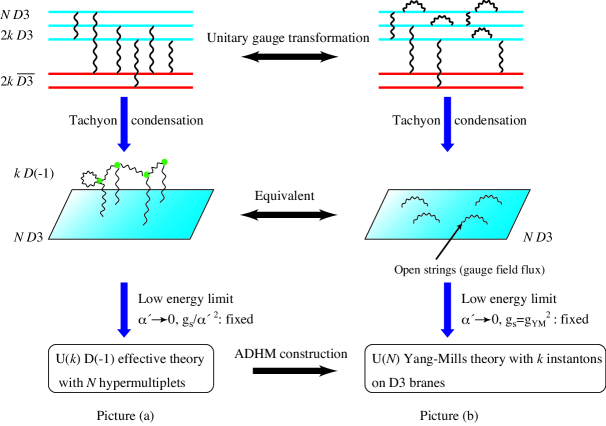
Figure 1: A sketch of the whole structure. In the middle, the left describes $D(-1)$-$D3$ bound state with DN- and DD-open strings, while the right one is $D3$-branes with open strings on them. Both are realized in $D3$/$\overline{D3}$-system and are gauge equivalent with each other. In the low energy limit, each reduces to the effective theory on the $D(-1)$-branes (picture (a)) and the $D3$-branes (picture (b)), respectively. The relation at the low energies is the ADHM construction.

Following the basic prescription of [18], we pay attention to the difference of roles of the gauge transformation and the tachyon condensation. Here, let us briefly summarize our strategy (see Fig. 1). We investigate the tachyon condensation of the system of $(N+2k)D3$-branes and $2k\overline{D3}$-branes in two ways corresponding to the pictures (a) and (b). We first consider the tachyon profile representing individual $kD(-1)$-branes and $ND3$-branes and add fluctuations of open strings ending on $D(-1)$-branes (DD-strings and DN-strings). This is the picture (a) where the system is regarded as a $kD(-1)$-$ND3$ bound state with open strings between them. Next, we consider a unitary transformation in the $D3$/$\overline{D3}$-system that shuffles the Chan-Paton indices of $(N+2k)D3$-branes. We show that new set of $2kD3$/$\overline{D3}$-branes completely annihilate into the vacuum under the tachyon condensation and instead the $k$-instanton gauge field (NN strings) appears on the remaining $ND3$-branes. This gives the picture (b) where the system is regarded as $N$ $D3$-branes with open strings. Since the two pictures are gauge equivalent with each other in the $D3/\overline{D3}$ system, they are different realizations of the same system. From this point of view, the ADHM construction is understood as a one-to-one correspondence between different low energy limits of the pictures (a) and (b).

Our novel departures in this paper are in the following. First, we show that the mechanism to produce a non-trivial gauge flux on the remaining $D$-branes presented in [18] is not restricted to the ADHM construction but a general consequence of the rectangular tachyon. Next, we explicitly present the concrete expression for the gauge transformation on the $D3/\overline{D3}$-brane system and take into account the worldsheet fermions not only the bosons, which are already promised in [19, 18]. As a result, we find that the completeness condition of the ADHM construction appears naturally so that the remaining gauge configuration is shown to be self-dual. It also guarantees the correct RR-charges. Moreover, the non-existence of the gauge transformation is shown to correspond to the small instanton singularity which spoils the ADHM construction of the self-dual gauge field strength. Finally, we emphasize the physical interpretation of the procedure based on the concept of “picture” explained above. The physical meaning of the ADHM construction becomes even clearer by introducing this concept. The relation between boundary states and low energy effective theory, the moduli space in terms of boundary states and the treatment of off-shell boundary states are easily understood.

The above arguments are not only specialized for the $D(-1)$-$D3$ bound state but also can be applied to other kind of D-brane bound states with even codimensions. Thus we will start from generic discussions on $Dp$/$\overline{Dp}$ system with $p+1=2n$, and after that we will go into the details of a specific bound state. In the low energy limit (of the picture (b)), the bound state would correspond to a BPS soliton if we impose the BPS condition to the system. In this way, we can apply our method to construct BPS solitons in principle.

The organization of the paper is as follows. In the next section, we briefly give generic arguments on the tachyon condensation in the system of the different number of $Dp$-branes and $\overline{Dp}$-branes in terms of the boundary state and review the construction of $D(-1)$-branes via the tachyon condensation as a preliminary of the discussion in the following section. In the section 3, we give a general mechanism to produce a non-trivial gauge configuration on the remaining $NDp$-branes after the tachyon condensation. In the section 4, we apply the procedure of the section 3 to the case of $p=3$. We express the $D(-1)$-$D3$ bound state in both of the pictures (a) and (b), and show that they are gauge equivalent with each other in the full string theory. We see that a gauge field naturally appears from the gauge transformation and it becomes an instanton gauge field if we impose the BPS condition. We also discuss the small instanton singularities and off-shell configurations of the bound state. In the section 5, we apply our method to other kinds of D-brane bound states. We discuss the relation between the bound state and higher dimensional instantons. We show that the $8$-dimensional version of the ADHM construction given in [20] is reproduced from our method.

2 Tachyon Condensation in $Dp$/$\overline{Dp}$ system

In this section, we would like to discuss general properties on the tachyon condensation of the different numbers of the $Dp$/$\overline{Dp}$ system in terms of the (off-shell) boundary state formalism. It is a straightforward generalization of [16], and is closely related to the boundary string field theory (BSFT) [21][22].

2.1 $Dp$/$\overline{Dp}$ system in terms of the boundary state

Let us first introduce the boundary states for $(N+M)Dp$-branes and $M\overline{Dp}$-branes in the Type II superstring theory. The boundary state is a state in the closed string Hilbert space defined by

$$\left|\,{Bp}\,\right\rangle_{\rm NS(RR)}\equiv\int[d{\mathbf{X}}^{\mu}]\left|\,{{\mathbf{X}}^{\mu},{\mathbf{X}}^{i}=0}\,\right\rangle_{\rm NS(RR)},$$ (2.1)

where $\mu=0,\cdots,p$ and $i=p+1,\cdots,9$ represent the worldvolume and the transverse directions of the $Dp$-branes, respectively. $\left|\,{{\mathbf{X}}^{M}}\,\right\rangle_{\rm NS(RR)}$ $(M=(\mu,i))$ are the eigenstates of the worldsheet closed string superfields restricted on the boundary,

$${\mathbf{X}}^{M}(\widehat{\sigma})=X^{M}(\sigma)+\sqrt{\alpha^{\prime}}\theta\Psi^{M}(\sigma),$$ (2.2)

in the NSNS(RR)-sector. In this paper we set $\alpha^{\prime}=1$. In (2.2), the superfields are functions in the boundary super coordinate $\widehat{\sigma}=(\sigma,\theta)$ unifying the worldsheet bosonic coordinate $0\leq\sigma<2\pi$ and its super-partner $\theta$. We have omitted the ghost contribution and the sign $\pm$ for the spin structure since they play no role for our purpose. The boundary state (2.1) represents the Neumann boundary condition for the $\mu$ direction while the Dirichlet one for the $i$ direction.

The open string degrees of freedom on the D-branes are introduced through the boundary interaction $S_{b}$ acting on the boundary state as

$$e^{-S_{b}}\left|\,{Bp}\,\right\rangle_{\rm NS(RR)},$$ (2.3)

where $e^{-S_{b}}$ has the form,

$$e^{-S_{b}}\equiv\begin{cases}{\rm Tr\,}\widehat{P}e^{\int d\widehat{\sigma}\mathbf{M}(\widehat{\sigma})}&\quad\text{(NSNS)},\\ {\rm Str\,}\widehat{P}e^{\int d\widehat{\sigma}\mathbf{M}(\widehat{\sigma})}&\quad\text{(RR)},\end{cases}$$ (2.4)

through a matrix $\mathbf{M}(\widehat{\sigma})$. $\widehat{P}$ in (2.4) denotes the super path-ordered product,

$$\widehat{P}e^{\int d\widehat{\sigma}\mathbf{M}(\widehat{\sigma})}\equiv 1+\sum_{n=1}^{\infty}(-1)^{\frac{n(n-1)}{2}}\int d\widehat{\sigma}_{1}\cdots d\widehat{\sigma}_{n}\Theta(\widehat{\sigma}_{1}-\widehat{\sigma}_{2})\cdots\Theta(\widehat{\sigma}_{n-1}-\widehat{\sigma}_{n})\mathbf{M}(\widehat{\sigma}_{1})\cdots\mathbf{M}(\widehat{\sigma}_{n}),$$ (2.5)

with the supersymmetric Heaviside function, $\Theta(\widehat{\sigma}-\widehat{\sigma}^{\prime})\equiv\theta(\sigma-\sigma^{\prime})-\theta\theta^{\prime}\delta(\sigma-\sigma^{\prime})$. In the system with $(N+M)Dp$-branes and $M$ $\overline{Dp}$-branes, the Chan-Paton Hilbert space is $(N+2M)$-dimensional complex vector space, so that, $\mathbf{M}(\widehat{\sigma})$ is an $(N+2M)\times(N+2M)$ matrix. Then the trace (2.4) in the NSNS-sector is taken over the Chan-Paton space ${\mathbb{C}}^{N+2M}$. It also possesses a ${\mathbb{Z}}_{2}$-grading with respect to the sign for the RR-charge. Then the super-trace in the RR-sector of (2.4) is defined by inserting the grading operator $\Gamma$:

$${\rm Str\,}(\widehat{P}\cdots)={\rm Tr\,}(\Gamma\widehat{P}\cdots),\qquad\Gamma=\left(\begin{array}[]{cc}{\mathbf{1}}_{N+M}&0\\ 0&-{\mathbf{1}}_{M}\end{array}\right).$$ (2.6)

We sometimes write $\mathbf{M}(\widehat{\sigma})$ in components with respect to $\theta$ as

$$\mathbf{M}(\widehat{\sigma})=M_{0}(\sigma)+\theta M_{1}(\sigma).$$ (2.7)

Using these component matrices, we can carry out $\theta$ integral in the definition of the boundary interaction (2.4), then it becomes

$$\widehat{P}e^{\int d\widehat{\sigma}\mathbf{M}(\widehat{\sigma})}=Pe^{\int d\sigma M(\sigma)},$$ (2.8)

with

$$M(\sigma)\equiv M_{1}(\sigma)-M_{0}(\sigma)^{2},$$ (2.9)

where $P$ now stands for the standard path-ordered product.

An important property is that this system has $U(N+M)\!\times\!U(M)$ gauge symmetry. The boundary interaction (2.4) is invariant under the gauge transformation of the form,

$$\mathbf{M}\to\mathbf{M}^{\prime}=-U({\mathbf{X}})^{\dagger}DU({\mathbf{X}})+U({\mathbf{X}})^{\dagger}\mathbf{M}U({\mathbf{X}}),$$ (2.10)

with

$$U({\mathbf{X}})=\left(\begin{array}[]{cc}U_{1}({\mathbf{X}})&0\\ 0&U_{2}({\mathbf{X}})\end{array}\right),\qquad U_{1}\in U(N+M),\ \ U_{2}\in U(M),$$ (2.11)

where $D=\partial_{\theta}+\theta\partial_{\sigma}$ is the boundary super-derivative and $U_{1}(U_{2})$ is an arbitrary functional of ${\mathbf{X}}^{\mu}$ valued in $U(N\!+\!M)(U(M))$, respectively. The first term in (2.10) is necessary for the invariance which comes from the definition of the super path-ordering (2.5). It is a super-analog of the gauge invariance of the Wilson loop operator (for the proof see Appendix A).

When we are interested in the massless and tachyonic excitations of open strings on this system, $\mathbf{M}$ can be written as

$$\mathbf{M}=\left(\begin{array}[]{cc}A_{\mu}({\mathbf{X}}^{\mu})D{\mathbf{X}}^{\mu}+\Phi^{i}({\mathbf{X}}^{\mu})\mathbf{P}_{i}&T({\mathbf{X}}^{\mu})\\ T({\mathbf{X}}^{\mu})^{\dagger}&\widetilde{A}_{\mu}({\mathbf{X}}^{\mu})D{\mathbf{X}}^{\mu}+\widetilde{\Phi}^{i}({\mathbf{X}}^{\mu})\mathbf{P}_{i}\end{array}\right),$$ (2.12)

where $\mathbf{P}_{i}$ is the conjugate momentum operator for ${\mathbf{X}}^{i}$. It represents boundary insertions of the massless and tachyon vertex operators with coefficient as corresponding fields on the $Dp$-branes. In our situation, the gauge field $A_{\mu}$ and scalar fields $\Phi_{i}$ ($\widetilde{A}_{\mu}$ and $\widetilde{\Phi}_{i}$) on the $Dp$-branes ($\overline{Dp}$-branes) are valued in ${(N+M)}\!\times\!{(N+M)}$ (${M}\!\times\!{M}$) matrices, respectively, which are transformed in the adjoint representation of the gauge group $U(N+M)$ and $U(M)$, respectively. Similarly the tachyon field $T$ connecting between the $Dp$-branes and the $\overline{Dp}$-branes is valued in $(N+M)\!\times\!{M}$ complex matrix which is transformed in the bi-fundamental representation $(N+M,\bar{M})$ of $U(N+M)\!\times\!U(M)$.

Since we would like to consider the situation that the initial massless fluctuation is absent and the only tachyon field is turned on, we simply drop the other fluctuation except for tachyon in (2.12) as

$$\mathbf{M}=\left(\begin{array}[]{cc}0&T({\mathbf{X}})\\ T({\mathbf{X}})^{\dagger}&0\end{array}\right),$$ (2.13)

which also gives rise to $M$ in (2.9) as

$$M=\left(\begin{array}[]{cc}-TT^{\dagger}(X)&\Psi^{\mu}\partial_{\mu}T(X)\\ \Psi^{\mu}\partial_{\mu}T^{\dagger}(X)&-T^{\dagger}T(X)\end{array}\right).$$ (2.14)

By a gauge transformation (2.10), this term (2.13) transforms into

$$\mathbf{M}^{\prime}=\left(\begin{array}[]{cc}-U_{1}^{\dagger}({\mathbf{X}})DU_{1}({\mathbf{X}})&U_{1}^{\dagger}({\mathbf{X}})T({\mathbf{X}})U_{2}({\mathbf{X}})\\ U_{2}^{\dagger}({\mathbf{X}})T^{\dagger}({\mathbf{X}})U_{1}({\mathbf{X}})&-U_{2}^{\dagger}({\mathbf{X}})DU_{2}({\mathbf{X}})\end{array}\right).$$ (2.15)

Comparing this with (2.12), we find that gauge fields appear on each of $Dp$-branes and $\overline{Dp}$-branes after the gauge transformation, but they are pure gauge because $-U_{1}({\mathbf{X}})^{\dagger}DU_{1}({\mathbf{X}})=-(U_{1}^{\dagger}\partial_{\mu}U_{1})({\mathbf{X}})D{\mathbf{X}}^{\mu}$. It plays an important role when we discuss the gauge flux production in the next section.

The boundary state carries all the information on the system. In particular it represents the coupling to any closed string state. Restricting to the coupling to massless closed string states and taking appropriate $\alpha^{\prime}\rightarrow 0$ limit, we obtain the low energy effective theory. From the discussion of the BSFT, the effective action for the tachyon field is given by

$$S[T]={}_{\rm NS}\!\left\langle\,{0}\,\right|{\rm Tr\,}\widehat{P}e^{\int d\widehat{\sigma}\mathbf{M}(\widehat{\sigma})}\left|\,{Bp}\,\right\rangle_{\rm NS},$$ (2.16)

where the $\mathbf{M}$ is defined as (2.13). It is equivalent to the disk partition function with any number of tachyon insertions. The explicit form of the action is obtained essentially by evaluating the bracket of the closed string Hilbert space and performing the functional integral in (2.1) but it is in general hard task. For the same number of $Dp$-branes and $\overline{Dp}$-branes ($N=0$), it is obtained in a closed form in [21, 22] in the derivative expansion up to ${\cal O}(\partial^{2}T)$. For $N\neq 0$, there are also some attempts [14]. Similarly, the Chern-Simons term can be written as

$$S_{\rm CS}[T]={}_{\rm RR}\!\left\langle\,{C}\,\right|{\rm Str\,}\widehat{P}e^{\int d\widehat{\sigma}\mathbf{M}(\widehat{\sigma})}\left|\,{Bp}\,\right\rangle_{\rm RR},$$ (2.17)

where $\left\langle\,{C}\,\right|$ is defined as a summation of the states of RR-forms,

$${}_{\rm RR}\!\left\langle\,{C}\,\right|\equiv\sum_{r}{}_{\rm RR}\!\left\langle\,{C_{r+1}}\,\right|.$$ (2.18)

For the RR-sector, the integration over the non-zero modes of the bosonic field $X^{M}$ and the fermionic field $\Psi^{M}$ cancel completely because of the worldsheet supersymmetry. Therefore the functional integral in (2.17) reduces to the usual integral of the bosonic zero modes $x^{\mu}$ and the fermionic zero modes play the role of the basis of differential forms $dx^{\mu}$ [21, 22]. Thus the Chern-Simons term (2.17) becomes

$$S_{\rm CS}=T_{p}\int C\wedge{\rm Str\,}e^{2\pi{\cal{F}}},$$ (2.19)

where $T_{p}$ is the tension of a $Dp$-brane and ${\cal F}$ is a supercurvature of the superconnection ${\cal A}$ on the (${\mathbb{Z}}_{2}$-graded) Chan-Paton bundle on ${\mathbb{R}}^{4}$. For (2.13), the superconnection ${\cal A}$ and the supercurvature ${\cal F}$ are given by

$${\cal A}=\left(\begin{array}[]{cc}0&T\\ T^{\dagger}&0\end{array}\right),\quad{\cal F}=\left(\begin{array}[]{cc}-TT^{\dagger}&\partial_{\mu}Tdx^{\mu}\\ \partial_{\mu}T^{\dagger}dx^{\mu}&-T^{\dagger}T\end{array}\right).$$ (2.20)

2.2 RR-charges and some simple examples without fluctuations

We can extract the qualitative feature on the tachyon condensation from the boundary interaction or the effective action above. First of all, let us consider the conserved RR-charge of $Dp$-branes after the tachyon condensation.

From (2.19), we find the $Dp$-brane charge coupled with RR $(p+1)$-form is obtained from the 0-form part in expansion of ${\rm Str\,}e^{2\pi{\cal F}}$,

$$Q_{p}={\rm Str\,}e^{-2\pi{\cal A}^{2}}={\rm Tr}_{N+M}\,e^{-2\pi TT^{\dagger}}-{\rm Tr}_{M}\,e^{-2\pi T^{\dagger}T}.$$ (2.21)

This just gives “index” of the superconnection ${\cal A}$ in (2.20) which is very analogous to the index of the Dirac operator. Indeed, as similar to the index theorem on the Dirac operator, we can easily see that eigenvalues of $TT^{\dagger}$ and $T^{\dagger}T$ are exactly the same except for $N$ zero eigenvalues included in $TT^{\dagger}$. Therefore we find

$$Q_{p}=N,$$ (2.22)

as expected. Note that the $Dp$-brane charge does not depend on any detail of the non-vanishing eigenvalues of $T^{\dagger}T$ or $TT^{\dagger}$, namely, the charge is topologically conserved independent of the fluctuations of tachyons.

Next, we look at the effective action (2.16) in the NSNS-sector. Irrespective of the detailed form of the kinetic term, the tachyon potential should take the form,

$$V(T)=T_{p}{\rm Tr\,}\exp 2\pi\left(\begin{array}[]{cc}-TT^{\dagger}&0\\ 0&-T^{\dagger}T\end{array}\right).$$ (2.23)

For a constant tachyon profile, the effective action (2.16) is exactly given by $S[T]=\int d^{p+1}xV(T)$. The potential minimum roughly exists at $|T|=\infty$. For example, if the tachyon has the constant profile as

$$T=\left(\begin{array}[]{c}0\\ u\,\ {\mathbf{1}}_{M}\end{array}\right),\qquad u\in{\mathbb{R}},$$ (2.24)

then the $2M\!\times\!2M$ part of the potential goes to the minimum in the limit $u\to\infty$. This means that $M$ pairs of $Dp$-branes and $\overline{Dp}$-branes decay into the vacuum and $NDp$-branes remain. This is also confirmed in terms of the boundary state,

$$e^{-S_{b}}\left|\,{p}\,\right\rangle_{\rm NS(RR)}\rightarrow N\left|\,{Bp}\,\right\rangle_{\rm NS(RR)}.$$ (2.25)

The final state carries the same value of the mass and the $Dp$-brane charge proportional to $NT_{p}$, thus it is a BPS state.

Now we derive the tachyon condensation to the system of $NDp$-branes and $kD(-1)$-branes, which carry RR $0$-form charge proportional to $kT_{-1}$ in addition to the RR $(p+1)$-form charge. Since the $D(-1)$-brane is a defect with the codimension $2n=p+1$ on the $Dp$-branes, it is obtained from the $2^{n-1}k$ pairs of $Dp$-branes and $\overline{Dp}$-branes by the well-known ABS construction [23]. It is embedded in our tachyon by setting $M=2^{n-1}k$ as

$$T({\mathbf{X}})=\left(\begin{array}[]{c}0\\ -u{\mathbf{X}}^{\mu}\gamma_{\mu}\otimes{\mathbf{1}}_{k}\end{array}\right),$$ (2.26)

where $\gamma_{\mu}$ are $2^{n-1}\times 2^{n-1}$ chiral parts of the even dimensional gamma matrices,

$$\Gamma_{\mu}=\left(\begin{array}[]{cc}0&\gamma_{\mu}\\ \gamma_{\mu}^{\dagger}&0\end{array}\right).$$ (2.27)

This profile breaks the gauge group down to $U(N)\times U(k)$. The tachyon potential has the form of a gaussian distribution,

$$V(T)=T_{p}{\rm Tr\,}\exp 2\pi\left(\begin{array}[]{ccc}0&0&0\\ 0&-u^{2}|x|^{2}\otimes{\mathbf{1}}_{2^{n-1}k}&0\\ 0&0&-u^{2}|x|^{2}\otimes{\mathbf{1}}_{2^{n-1}k}\\ \end{array}\right).$$ (2.28)

Suggested by the gaussian nature, $2^{n-1}k$ pairs of $Dp$-branes and $\overline{Dp}$-branes disappears outside the core, $|x|>1/u$, and some defect remains inside the core, $|x|<1/u$, since the potential does not vanish. To show (2.26) gives the $kD(-1)$ solution in the effective action, now the kinetic term in (2.16) is also important in addition to the potential term, because (2.26) is space dependent. Roughly speaking, both contributions give the correct $\delta$-function as ${\text{(}potential)}\times{\text{(}kinetic)}=(\frac{\delta^{(4)}(x)}{u^{4}})\times(u^{4})$ in the limit $u\to\infty$ [21]. It is indeed seen at the level of boundary states by inserting (2.26) into the matrix $\mathbf{M}$ (2.13): one can show that this system has $NDp$-brane charge and $k$ D(-1)-brane charge in the RR-sector even when $u$ is finite, while in the NSNS sector bosonic zero-mode part indicates that the defect has gaussian distribution with the size $|x|\sim 1/u$ and the mass is larger than that of $k$ D(-1)-branes [24]. In the limit $u\to\infty$, we have

$$e^{-S_{b}}\left|\,{Bp}\,\right\rangle_{\rm NS(RR)}\rightarrow N\left|\,{Bp}\,\right\rangle_{\rm NS(RR)}+k\left|\,{B(-1)}\,\right\rangle_{\rm NS(RR)},$$ (2.29)

where $\left|\,{B(-1)}\,\right\rangle=\left|\,{{\mathbf{X}}^{M}=0}\,\right\rangle$ is a boundary state of Dirichlet boundary condition for all directions. Therefore, this gives the tachyon condensation from $2^{n-1}k$ pairs of $Dp$/$\overline{Dp}$-branes to $k$ D(-1)-branes at the origin, while keeping $NDp$-branes unchanged.

3 Gauge Flux Production by Unitary Transformations

The characteristic feature of the system of $(N\!+\!M)Dp$-branes and $M\overline{Dp}$-branes is that the tachyon field is valued in rectangular matrices. The condensation of such a tachyon becomes important in the later discussion for the D-brane bound states. In some cases, the pair of $MDp$-branes and $M\overline{Dp}$-branes decay into the vacuum, and the information on the tachyon profile is completely converted to the gauge field profile on the $NDp$-branes. In this section, we describe this mechanism.

To this end, let us consider an arbitrary tachyon profile $T({\mathbf{X}})$ in (2.13) as an $(N+M)\!\times\!M$ complex matrix valued function. We assume that it is proportional to the parameter $u$. Roughly speaking, the structure of the tachyon condensation is determined by the behavior of the tachyon potential (2.23) under the limit $u\rightarrow\infty$. Since the tachyon potential is invariant under the gauge symmetry $U(N+M)\!\times\!U(M)$, we can choose a suitable basis for the trace and rearrange the Chan-Paton indices so as to separate them into two classes; $Dp$-branes which may annihilate and $Dp$-branes which always remain after the tachyon condensation.

The combination $TT^{\dagger}(x)$ and $T^{\dagger}T(x)$ appears in (2.23) are scalar function on ${\mathbb{R}}^{p+1}$, which are valued in hermitian matrices with the sizes of $(N+M)\!\times\!(N+M)$ and $M\times M$ and transformed in the adjoint representation of $U(N+M)$ and $U(M)$, respectively. An immediate consequence is that, at any point in ${\mathbb{R}}^{4}$, $TT^{\dagger}$ has at least $N$ zero eigenvalues and the other $M$ eigenvalues completely coincide to those of $T^{\dagger}T$. Therefore, we can bring $TT^{\dagger}$ to the block diagonal form using a unitary matrix $U_{1}(x)\in U(N+M)$;

$$U_{1}^{\dagger}TT^{\dagger}U_{1}=\left(\begin{matrix}0&0\\ 0&T^{\dagger}T\end{matrix}\right).$$ (3.1)

Note that the hermitian matrix $T^{\dagger}T$ is positive semi-definite, that is, its all eigenvalues $\lambda_{l}\,(l=1,\cdots M)$ are non-negative. Then, its square-root is also an $M\times M$ hermitian matrix, but here the eigenvalues are $\pm\sqrt{\lambda_{l}}$, that is, there is the $2^{M}$ degeneracy. By choosing the positive root for all eigenvalues, we can define the square-root denoted as

$$\lambda\equiv\left(T^{\dagger}T\right)^{1/2}.$$ (3.2)

The other sign choices are recovered by applying $({\mathbb{Z}}_{2})^{M}$ transformation, which is a discrete subgroup of $U(M)$.

Furthermore, in this section, we assume that the matrix $T^{\dagger}T$ is strictly positive at any point in ${\mathbb{R}}^{4}$. This guarantees that $\lambda$ has its inverse $\lambda^{-1}$. Under this assumption, we can easily find the explicit form of $U_{1}$ as follows. First, we decompose the matrix $U_{1}$ by collections of $N$ and $M$ vectors in ${\mathbb{C}}^{N+M}$, respectively, as

$$U_{1}=\left(V,W\right),$$ (3.3)

where $V$ is a collection of $N$ normalized zero eigenvectors of $T^{\dagger}$,

$$T^{\dagger}V =0,$$ (3.4)

$$V^{\dagger}V ={\mathbf{1}}_{M},$$ (3.5)

and $W$ is a collection of $M$ normalized vectors defined by using the existence of $\lambda^{-1}$ as

$$W=T{\lambda}^{-1},$$ (3.6)

since $W$ are arranged so as $TT^{\dagger}W=WT^{\dagger}T$. Then the conditions for $U_{1}$ to be unitary matrix,

$$U_{1}^{\dagger}U_{1}=\left(\begin{matrix}V^{\dagger}V&V^{\dagger}T{\lambda}^{-1}\\ {\lambda}^{-1}T^{\dagger}V&{\lambda}^{-1}T^{\dagger}T{\lambda}^{-1}\\ \end{matrix}\right)=\left(\begin{matrix}{\mathbf{1}}_{N}&0\\ 0&{\mathbf{1}}_{M}\\ \end{matrix}\right),$$ (3.7)

$$U_{1}U_{1}^{\dagger}=VV^{\dagger}+T{\lambda}^{-2}T^{\dagger}={\mathbf{1}}_{N+M},$$ (3.8)

are automatically satisfied because these vectors span the orthonormal basis. It is also easy to see (3.1) is satisfied. Having found a specific unitary matrix $U_{1}$ (3.3), there is still a residual symmetry $U(N)\!\times\!({\mathbb{Z}}_{2})^{M}\subset U(N+M)$, which keeps (3.1) invariant. It acts on $U_{1}$ as

$$U_{1}=\left(V,W\right)\,\,\rightarrow\,\,(VR,WS)\qquad R\in U(N),\,\,S\in({\mathbb{Z}}_{2})^{M},$$ (3.9)

where the second factor $S$ is the degeneracy stated above.

Some remarks are in order. In general, both $V$ and $W$ depend on the points in ${\mathbb{R}}^{p+1}$ since $TT^{\dagger}(x)$ is a function on ${\mathbb{R}}^{p+1}$. It is worth to note at this stage that the conditions (3.4), (3.5) and (3.8) are the same as the equations appearing in the ADHM construction (when $p=3$ and $M=2k$). The first two conditions (3.4) and (3.5) means that $V$ is the normalized zero-modes of the “Dirac operator” $T^{\dagger}$. The last one (3.8), called the completeness relation, says that $VV^{\dagger}$ and $T{\lambda}^{-2}T^{\dagger}$ are the orthogonal projection operator onto the $N$ and $M$ dimensional subspace of ${\mathbb{C}}^{N\!+\!M}$, respectively. We will argue the precise correspondence in the next section. Note also that $W$ is independent of the parameter $u$ because $T\propto u$ and $\lambda^{-1}\propto u^{-1}$. Therefore, the gauge transformation $U_{1}$ is also independent of $u$.

What we have done is shuffling the $(N\!+\!M)Dp$-branes and relabelling the Chan-Paton indices such that the tachyon and its potential has the form,

$$T^{\prime}=U_{1}^{\dagger}T=\left(\begin{matrix}0\\ \lambda\\ \end{matrix}\right),\qquad V(T^{\prime})=T_{3}\,{\rm Tr\,}\exp\left(\begin{matrix}0&0&0\\ 0&-\lambda^{2}&0\\ 0&0&-\lambda^{2}\\ \end{matrix}\right).$$ (3.10)

Now this tachyon profile is to be compared with that of (2.24) and (2.26). Although $\lambda^{2}(x)$ depends on the space coordinate, their eigenvalues are strictly positive at any point in ${\mathbb{R}}^{p+1}$ so that the tachyon potential behaves similarly as (2.24). Then, under this condition, it is expected that the $M$-pairs of $Dp$-branes and $\overline{Dp}$-branes completely disappear and $NDp$-branes keep alive in the limit of $u\to\infty$. If we want to know more details of the tachyon condensation, we should also evaluate the kinetic term not only the potential term as for the case of (2.26) since the tachyon profile depends on the spacetime coordinate. Unfortunately, however, it is quite hard task in general since we do not know the explicit form of the effective action.

So far we restrict the discussion only on the tachyon potential in order to sketch the behavior of the system. However, we can treat the system more precisely using the boundary state formalism. The main difference is that the gauge invariant object is now the boundary interaction $e^{-S_{b}}$ (2.4) and the unitary transformation induces inevitably the pure gauge connection (2.10) in the boundary interaction. We now look at the same gauge transformation at the level of boundary state and see how the (non-trivial) gauge field appears. Let us consider the boundary interaction with $\mathbf{M}$ (2.13). Among the gauge symmetry $U(N+M)\!\times\!U(M)$, the gauge function (2.11) of our concern is given by

$$U({\mathbf{X}})\equiv\left(\begin{matrix}U_{1}({\mathbf{X}})&0\\ 0&{\mathbf{1}}_{M}\\ \end{matrix}\right),$$ (3.11)

where $U_{1}\in U(N\!+\!M)$ is given by (3.3). Note that it is a functional of the string (super)coordinate ${\mathbf{X}}^{\mu}(\widehat{\sigma})$. Then the corresponding gauge transformation (2.10) for $\mathbf{M}$ is

$$\mathbf{M}\mapsto\mathbf{M}^{\prime}=\mathbf{P}+\mathbf{A},$$ (3.12)

where

$$\mathbf{P}\equiv U^{\dagger}\mathbf{M}U=\left(\begin{matrix}0&0&0\\ 0&0&\lambda\\ 0&\lambda&0\end{matrix}\right),\qquad\mathbf{A}\equiv-U^{\dagger}DU=\left(\begin{matrix}-V^{\dagger}DV&-V^{\dagger}DW&0\\ -W^{\dagger}DV&-W^{\dagger}DW&0\\ 0&0&0\end{matrix}\right).$$ (3.13)

The first term $\mathbf{P}$ comes from the adjoint action of $U({\mathbf{X}})$ acting on $\mathbf{M}$. This term reduces to the transformation law (3.10) in the effective theory. The second term $\mathbf{A}$ is the induced pure gauge connection by the transformation $U({\mathbf{X}})$.

Recalling (2.12), $\mathbf{A}$ represents an insertion of the massless gauge fields on the $(N\!+\!M)D3$-branes. Initially, the gauge transformation is introduced to block-diagonalize the tachyon potential, but it also decomposes $\mathbf{M}^{\prime}$ into a tachyon part $\mathbf{P}$ and a gauge field part $\mathbf{A}$. It says that not all the component of the initial tachyon profile are indeed tachyonic. Note also that $\mathbf{P}$ is $u$-dependent while $\mathbf{A}$ is $u$-independent. In general, only the $u$-dependent part is responsible for the tachyon condensation $u\rightarrow\infty$, while the others are regarded as fluctuations around the condensed vacuum. Such a decomposition is not only for the convenience but also relies on the physical interpretation of the system after the tachyon condensation. There is a case where we can further extract $u$-independent parts from $\mathbf{P}$ which are regarded as fluctuations, but it heavily relies on the detailed form of the tachyon profile. We will come back to this point in the section 4.5. Hence in this section, we simply treat $\mathbf{P}$ as the principal part of the tachyon condensation (background) and $\mathbf{A}$ as a fluctuation. Correspondingly, in evaluating the boundary interaction, it is convenient to use the following identity for the (super)path-ordered product (for the proof see the appendix B),

$$\widehat{P}e^{\int d\widehat{\sigma}\mathbf{M}(\widehat{\sigma})} =\widehat{P}e^{\int d\widehat{\sigma}(\mathbf{P}(\widehat{\sigma}))+\mathbf{A}(\widehat{\sigma}))}$$

$$\equiv\widehat{P}e^{\int d\widehat{\sigma}\mathbf{P}(\widehat{\sigma})}+\sum_{n=1}^{\infty}\int d\widehat{\sigma}_{1}\cdots d\widehat{\sigma}_{n}\mathbf{A}(\widehat{\sigma}_{n}){\mathbf{T}}_{\mathbf{P}}(\widehat{\sigma}_{n}-\widehat{\sigma}_{n-1})\mathbf{A}(\widehat{\sigma}_{n-1})$$

$$\hskip 142.26378pt\times{\mathbf{T}}_{\mathbf{P}}(\widehat{\sigma}_{n-1}-\widehat{\sigma}_{n-2})\cdots{\mathbf{T}}_{\mathbf{P}}(\widehat{\sigma}_{2}-\widehat{\sigma}_{1})\mathbf{A}(\widehat{\sigma}_{1}),$$ (3.14)

where the “transfer matrix” ${\mathbf{T}}_{\mathbf{P}}(\widehat{\sigma}^{\prime}-\widehat{\sigma})$ is defined only through $\mathbf{P}$ as

$${\mathbf{T}}_{\mathbf{P}}(\widehat{\sigma}^{\prime}-\widehat{\sigma})\equiv\widehat{P}e^{\int d\widehat{\sigma}^{\prime\prime}\mathbf{P}(\widehat{\sigma}^{\prime\prime})\left(\Theta(\widehat{\sigma}^{\prime}-\widehat{\sigma}^{\prime\prime})-\Theta(\widehat{\sigma}^{\prime\prime}-\widehat{\sigma})\right)}.$$ (3.15)

This identity means that inserting infinitely many numbers of the vertex operators $\mathbf{P}$ first, which fixes the background, and then inserting $\mathbf{A}$ as perturbations. ${\mathbf{T}}_{\mathbf{P}}(\widehat{\sigma}^{\prime}-\widehat{\sigma})$ is further estimated by expanding $\mathbf{P}$ with respect to $\theta$ as $\mathbf{P}(\widehat{\sigma})=P_{0}(\sigma)+\theta P_{1}(\sigma)$ and again using the similar identity for the standard path-ordering,

$${\mathbf{T}}_{\mathbf{P}}(\widehat{\sigma}^{\prime}-\widehat{\sigma}) =Pe^{\int_{\sigma}^{\sigma^{\prime}}d\sigma^{\prime\prime}(P_{1}(\sigma^{\prime\prime})-P_{0}^{2}(\sigma^{\prime\prime}))}$$

$$=T_{-P_{0}^{2}}(\sigma^{\prime}-\sigma)$$

$$\hskip 28.45274pt+\sum_{n=1}^{\infty}\int d\sigma_{1}\cdots d\sigma_{n}T_{-P_{0}^{2}}(\sigma^{\prime}-\sigma_{n})P_{1}(\sigma_{n})T_{-P_{0}^{2}}(\sigma_{n}-\sigma_{n-1})P_{1}(\sigma_{n-1})$$

$$\hskip 105.2751pt\times T_{-P_{0}^{2}}(\sigma_{n-1}-\sigma_{n-2})\cdots{T}_{-P_{0}^{2}}(\sigma_{2}-\sigma_{1})P_{1}(\sigma_{1}){T}_{-P_{0}^{2}}(\sigma_{1}-\sigma),$$ (3.16)

where

$$T_{-P_{0}^{2}}(\sigma^{\prime}-\sigma) \equiv Pe^{-\int_{\sigma}^{\sigma^{\prime}}d\sigma^{\prime\prime}P_{0}^{2}(\sigma^{\prime\prime})}$$

$$=\left(\begin{matrix}1&0&0\\ 0&Pe^{-\int d\sigma\lambda^{2}(X)}&0\\ 0&0&Pe^{-\int d\sigma\lambda^{2}(X)}\end{matrix}\right).$$ (3.17)

The main point is that $\lambda^{2}$ diverges uniformly (irrespective of $X(\sigma)\,$) in the limit of $u\to\infty$ since we have assumed that the matrix $\lambda$ is strictly positive definite and also that all the eigenvalues are $u$-dependent. Hence, it is concluded that (3.17) reduces to the projection operator onto the $N$-dimensional subspace of the $(N+M)$-dimensional Chan-Paton space in the limit $u\to\infty$:

$$T_{-P_{0}^{2}}(\sigma^{\prime}-\sigma)\stackrel{{\scriptstyle u\to\infty}}{{\longrightarrow}}\left(\begin{matrix}{\mathbf{1}}_{N}&0\\ 0&0\end{matrix}\right)\equiv{\cal P}_{N}.$$ (3.18)

Then, it is easy to see that (3.15) also goes to the same projection operator ${\cal P}_{N}$ under the limit $u\rightarrow\infty$. This is because each $P_{1}(\sigma)$ in (3.16) is now sandwiched by ${\cal P}_{N}$ but it vanishes (${\cal P}_{N}P_{1}(\sigma){\cal P}_{N}=0$). The fact that the condensation of the principal part $\mathbf{P}$ becomes the projection operator ${\cal P}_{N}$ supports the rough sketch of the behavior obtained from the tachyon potential. But we emphasize that this is true only under the assumption that whole $\mathbf{P}$ is relevant for the tachyon condensation.

We can further estimate (3.14) in the limit of $u\to\infty$ as the same manner: each $\mathbf{A}(\widehat{\sigma})$ are replaced by ${\cal P}_{N}\mathbf{A}(\widehat{\sigma}){\cal P}_{N}$ and we obtain

$$\widehat{P}e^{\int d\widehat{\sigma}\mathbf{M}(\widehat{\sigma})} \stackrel{{\scriptstyle u\to\infty}}{{\longrightarrow}}{\cal P}_{N}\left(\widehat{P}e^{\int d\widehat{\sigma}\mathbf{A}(\widehat{\sigma})}\right){\cal P}_{N}$$

$$=\widehat{P}\exp\left\{\int d\widehat{\sigma}\left(\begin{matrix}-V^{\dagger}DV&0\\ 0&0\end{matrix}\right)\right\}.$$ (3.19)

Therefore, in the limit $u\rightarrow\infty$, the boundary state reduces to

$$e^{-S_{b}}\left|\,{Bp}\,\right\rangle_{\rm NS(RR)}\rightarrow{\rm(S)Tr}_{N}\left(\widehat{P}e^{-\int d\widehat{\sigma}V^{\dagger}DV}\right)\left|\,{Bp}\,\right\rangle_{\rm NS(RR)}.$$ (3.20)

This means that the $M$ pairs of the $Dp$-branes and $\overline{Dp}$-branes completely disappear and only $NDp$-branes remain after the tachyon condensation ($u\to\infty$). Moreover, an $U(N)$ gauge connection,

$$A_{\mu}=-V^{\dagger}\partial_{\mu}V,$$ (3.21)

appears on the remaining $NDp$-branes since $V^{\dagger}DV=(V^{\dagger}\partial_{\mu}V)D{\mathbf{X}}^{\mu}$ (see (2.12)). The residual gauge symmetry $U(N)$ in (3.9) remains on the $NDp$-branes, which act on (3.21) as

$$A_{\mu}\mapsto A^{\prime}_{\mu}=R^{\dagger}\partial_{\mu}R+R^{\dagger}A_{\mu}R.$$ (3.22)

We have given the mechanism that the initial information on the tachyon profile is converted to the gauge profile (3.21) on the remaining $ND3$-branes. Since it is simply a gauge transformation, it gives a unitary equivalence between the $Dp/\overline{Dp}$-system with a tachyon and the $Dp$-branes with a flux. We emphasize that this mechanism is the consequence of the (non-vanishing) tachyon between the $NDp$-branes and $MDp/\overline{Dp}$-branes. In fact, for the tachyon profiles (2.24) and (2.26), we can not apply the transformation (3.1) (or it is trivial). As we will see in the next section, it is the essence of the bound state formation, where (3.21) corresponds to the $U(N)$ gauge connection in the ADHM construction. However, since it is pure gauge form, it seems to make no physical effect at first sight. In fact, at the level of the Chern-Simons term (2.19), the supercurvature transforms covariantly under $U(x)$ so that the non-trivial curvature seems not to be produced by such a gauge transformation. But it is not true in general. The point is that the unitary transformation could be a large gauge transformation, and moreover, even if the total curvature in the $U(N+M)$ is still trivial, the curvature projected onto the $U(N)$ part may be non-trivial, while the other part of $U(N+M)$ becomes hidden under the tachyon condensation. Whether (3.21) is in fact non-trivial or does not depend on the topological information carried by the gauge function $U({\mathbf{X}})$, or equivalently, the initial tachyon profile.

Before concluding this section, we give a few remarks. First of all, although we have used the transformation of the form (3.1), the argument in this section is unchanged if the $N$ zero-modes $V$ are successively separated. In other words, a further transformation of (3.10) by the $U(M)\times U(M)$ gives the same conclusion, because the induced pure gauge connection by this transformation is projected out by ${\cal P}_{N}$. Secondary, the argument relies only on the existence of the gauge transformation and the appropriate separation of the principal part. So it is also applicable to a case with initial non-vanishing massless fields by an appropriate generalization. In this case, they are not relevant for the tachyon condensation itself but we should be careful about the gauge symmetry breaking by them. Finally, if $T^{\dagger}T$ is not always positive, there should be zero modes at least at some space point. Even in this case, by separating zero-mode part and considering only the small matrix, a rearrangement such as (3.1) still works. As a consequence, we obtain after the transformation the system of $(N+M^{\prime})Dp$/$M^{\prime}\overline{Dp}$-branes with a flux, where $M^{\prime}(<M)$ is the number of the above zero-modes.

4 Instantons in the $D3$/$\overline{D3}$ system

In the previous section, we considered the system of coincident $(N+M)Dp$-branes and $M\overline{Dp}$-branes with a generic tachyon profile. In this section, we concentrate on the case of $(N+2k)D3$-branes and $2k\overline{D3}$-branes with tachyon profiles, which carry the $kD(-1)$-brane charge. We will show the physical equivalence between a system of $kD(-1)$-branes and $ND3$-branes with open strings stretched between them and a system of $ND3$-branes with a gauge flux through a unitary equivalence in the $D3$/$\overline{D3}$ system. This in particular explains the ADHM construction of the instantons in $4D$ gauge theory.

4.1 Two pictures of bound states

Let us first recall the fact about the $D(-1)$-$D3$ bound states described in the section 1 in slightly more detail. It is well known that the system of well separated $ND3$-branes and $kD(-1)$-branes preserves the spacetime supersymmetry. Furthermore, we can consider the collective excitations of them by turning on massless open strings. If $ND3$-branes and $kD(-1)$-branes are located closely with each other, stretched open strings between them become massless and the system forms a BPS bound state. It is known that this system is marginal bound state, that is, the total mass of the bound state equals to that of the individual $ND3$-branes and $kD(-1)$-branes. In the section 1, we present two physically equivalent ways to describe this BPS bound state in the superstring theory (see Fig. 1 in the section 1).

The first picture (a) is the system of coincident $ND3$-branes and $kD(-1)$-branes and massless open strings, whose ends are attached at least on the $D(-1)$-branes (DN- and DD-strings). Such open strings are the collective degrees of freedom that survive in the low energy limit of $\alpha^{\prime}\to 0$ with fixing the $0$-dimensional gauge coupling $g_{0}^{2}\sim g_{s}\alpha^{\prime-2}$. Here the excitations on $D3$-branes become extremely heavy and other massive excitations or gravitational interactions are decoupled. Then the effective theory on the $D(-1)$-branes becomes the $0$-dimensional supersymmetric gauge theory with gauge group $U(k)$ and flavor symmetry $U(N)$. The (bosonic) matter contents of this effective theory are in the following. From the massless excitation of open strings stretched between $D(-1)$-branes, there appear $10$ scalar fields $\Phi^{M}\,(M=0,1,\cdots,9)$ in the adjoint representation of $U(k)$, which describe the transverse positions of $D(-1)$-branes. Open strings between $D(-1)$-branes and $D3$-branes give scalar fields $H=(I^{\dagger},J)$ where $I$ and $J$ are in the $(\bar{N},{k})$ and $(N,\bar{k})$ representation of $U(N)\times U(k)$, respectively.

In terms of low energy effective theory, the BPS condition of the system is equivalent to the condition where the vacuum expectation value (vev) of matter fields lie in the supersymmetric vacua. The vacua of the theory have several branches. The Higgs branch, where the vev of the scalar fields $\Phi^{i}\,(i=4,\cdots,9)$ are zero while $H$ and $\Phi^{\mu},(\mu=0,1,2,3)$ have non-zero vev, corresponds to the situation where the $D(-1)$-branes are located inside the $D3$-branes. The Coulomb branch, where $H=0$ and $\Phi^{M}\neq 0$, describes the situation in which the $D(-1)$-branes move off the $D3$-branes. There are also mixed branches where some of the $D(-1)$-branes still lie on the $D3$-branes and other $D(-1)$-branes move off the $D3$-branes. If the field configurations lie on these flat directions, the system has the same mass as that of $ND3$-branes and $kD(-1)$-branes.

Another picture (b) is the system of $ND3$-branes with massless open strings excited on them (NN-strings). In this picture, the $kD(-1)$-branes are completely dissolved into the $ND3$-branes as a gauge field configuration. Therefore, this description is quite well compatible with instantons in the supersymmetric gauge theory. In fact, in the low energy limit $\alpha^{\prime}\to 0$ with fixing the $4$-dimensional gauge coupling $g_{4}^{2}\sim g_{s}$, the effective theory on the $ND3$-branes becomes the ${\cal N}=4$ $U(N)$ supersymmetric Yang-Mills theory with the Chern-Simons term, where the $kD(-1)$-branes charge is carried by the $k$-instanton gauge configuration through the coupling $C\int{\rm Tr\,}(F\wedge F)$. If we restrict ourselves to the vev for the $6$ transverse scalar fields $\Phi^{i}$ to be zero, the bosonic content of this theory is simply given by the $U(N)$ Yang-Mills theory with a $\theta$-term. Then the BPS condition (vacua) is equivalent to the self-dual field strength, where the Yang-Mills action is equal to the $k$-instanton action.

In the Higgs branch of the picture (a) and in the $k$-instanton sector of the picture (b), the mass (action) and the RR-charges of the BPS configurations are the same so that they are thought to be equivalent. However, this equivalence seems to be mysterious since they are defined in the very different low energy limit of the seemingly different D-brane systems with each other. Nevertheless, a remarkable correspondence between two pictures at low energy is provided by the ADHM construction [5, 7]. In this construction, the D and F-flatness condition defining the Higgs branch (ADHM equation) in the picture (a) is mapped to the self-dual condition in the picture (b). The instanton moduli space ${\cal M}_{N,k}$ in the picture (b) is also recovered by the ADHM data, $H$ and $\Phi^{\mu}$, divided by the auxiliary symmetry $U(k)$,

$${\cal M}_{N,k}=\{(H,\Phi^{\mu})|\mbox{ADHM eqs.}\}/U(k).$$ (4.1)

Moreover, singularities in the instanton moduli space ${\cal M}_{N,k}$, where we cannot construct a regular instanton gauge field (small instanton singularity), correspond to the conical singularities in the hyper-Kähler quotient (4.1). In the D-brane setting, this limit connects different branches in (a) and it is regarded as a stringy resolution of the small instanton singularity. This is the ordinary explanation of the ADHM construction in terms of the dynamics of D-branes in string theory.

In this paper, we show that the correspondence between the above two BPS systems is understood as a gauge equivalence. We also propose that the equivalence between (a) and (b) is not restricted on the low energy limits nor on the BPS configurations. Our strategy is summarized in the figure 1 in the section 1. First, we consider the D-brane system in the both pictures, where the only excitations are the low energy degrees of freedom. They are described in the full string theory by the boundary states with specific open string excitations, that is, $kD(-1)$-branes and $ND3$-branes with DN- and DD-strings in (a) and $ND3$-branes with NN-strings in (b). Next, each boundary state is obtained from the same system of $(N+2k)D3$-branes and $2k\overline{D3}$-branes as a result of the tachyon condensation. In the picture (a) $2k$ pairs of $D3$/$\overline{D3}$-branes give $kD(-1)$-branes, while in the picture (b) they are annihilated into the closed string vacuum. In the following subsections, we will construct the bound state of $N$ $D3$-branes and $kD(-1)$-branes in the both pictures using the tachyon condensation from a $D3$/$\overline{D3}$ system and we will show that the two descriptions are simply related by the unitary gauge transformation in $U(N+2k)\times U(2k)$, which is the mechanism described in the section 3. Therefore, two pictures arise as specific gauges and they are unitary equivalent with each other as the D-brane systems.

4.2 ADHM data as tachyon profile

In this subsection, we describe the picture (a), that is, a $kD(-1)$/$ND3$ bound state with open string excitations $H$ and $\Phi^{\mu}$ in terms of boundary state. The boundary states of individual $D3$-branes and $D(-1)$-branes is a linear combination of them as given by (2.29) with $p\!=\!3$. Excitations of $4$ scalar fields $\Phi^{\mu}$ are simply incorporated by the boundary interaction $e^{-S_{b}}$ acting on $\left|\,{B(-1)}\,\right\rangle$, which represents arbitrary number of boundary insertions of massless vertex operators on the disk with the Dirichlet boundary condition. More precisely, it has the form,

$$e^{-S_{b}}={\rm(S)Tr}_{k}\,\widehat{P}e^{-i\int d\widehat{\sigma}\Phi^{\mu}\mathbf{P}_{\mu}(\widehat{\sigma})}.$$ (4.2)

On the other hand, since $H$ is DN-strings connecting the $D3$-branes and $D(-1)$-branes, their insertions should be accompanied with the boundary condition changing operators or twist fields in general, which is not well developed so far to handle in the context of boundary state. However, there is another way to represent them: we come back to the system of $(N+2k)D3$-branes $2k\overline{D3}$-branes and add the fluctuations corresponding to $H$ and $\Phi^{\mu}$ around the $kD(-1)$-brane solution (2.26). Explicitly, it corresponds to the tachyon profile,

$$T({\mathbf{X}})=u\left(\begin{array}[]{c}H\\ (\Phi^{\mu}-{\mathbf{X}}^{\mu})\otimes\sigma_{\mu}\end{array}\right)=u\left(\begin{matrix}I^{\dagger}&J\\ {B}_{2}^{\dagger}-{{\mathbf{Z}}}_{2}^{\dagger}&-{B}_{1}+{{\mathbf{Z}}}_{1}\\ {B}_{1}^{\dagger}-{{\mathbf{Z}}}_{1}^{\dagger}&{B}_{2}-{{\mathbf{Z}}}_{2}\end{matrix}\right),$$ (4.3)

where $T$ is valued in $(N\!+\!2k)\times 2k$ matrix, $H$ is a complex $N\times 2k$ matrix, $\Phi_{\mu}\,(\mu=0,1,2,3)$ are hermitian $k\times k$ matrices, respectively. $\sigma_{\mu}$ are quotanion basis defined by $\sigma_{\mu}=(1,-i\tau_{i})$ using Pauli matrices $\tau_{i}\,(i=1,2,3)$. In the second expression of (4.3), we have introduced a complex notation where ${B}_{1,2}$ and ${{\mathbf{Z}}}_{1,2}$ are defined as

$${B}_{1}\equiv\Phi^{2}+i\Phi^{1},\qquad{B}_{2}\equiv\Phi^{0}+i\Phi^{3},$$ (4.4)

and

$${{\mathbf{Z}}}_{1}\equiv{\mathbf{X}}^{2}+i{\mathbf{X}}^{1},\qquad{{\mathbf{Z}}}_{2}\equiv{\mathbf{X}}^{0}+i{\mathbf{X}}^{3},$$ (4.5)

respectively. In this setting, $\Phi^{\mu}$ describe the degrees of freedom of open strings between $2kD3$-branes and $2k\overline{D3}$-branes. When $H=0$, the tachyon condensation of this profile (4.3) gives the boundary interaction (4.2) as expected [16] (see also the section 4.5). This means that $\Phi^{\mu}$ become the transverse scalar fields on $kD(-1)$-branes after the tachyon condensation. Similarly, $H$ in (4.3) corresponds to the open strings between the $ND3$-branes and the $2k$ pairs of $D3$/$\overline{D3}$-branes. Then it is natural to expect that it would describe the DN-strings between $D3$-branes and $D(-1)$-branes after the tachyon condensation.

This tachyon profile (4.3) is evidently proportional to the “Dirac operator” $\Delta$ in the canonical form in the context of the ADHM construction (see e.g. [7]), that is, $H$ and $\Phi^{\mu}$ are identified with the ADHM data and $T=u\Delta$. Such an identification is first appeared in the literature [17] to describe $D5$-branes inside the $D9$-branes in the context of the effective action. They have evaluated the Chern-Simons term (2.19) in the simplest example of $H$ and $\Phi^{\mu}$ ($N=2,\,k=1$) and confirmed that (4.3) possesses the correct RR-charge density expected from the instanton configuration. However, the ADHM equation (or D and F-flatness condition) itself cannot recovered only by the Chern-Simons term. In terms of boundary states, the BPS condition are seen by “mass = RR-charge” by evaluating both the BSFT action (2.16) and the Chern-Simons term (2.17). In this way the ADHM equation would be recovered in the boundary state formalism essentially. However, as emphasized in [18], it is difficult task to see whether the ADHM equation is the exact BPS condition which receives no $\alpha^{\prime}$-corrections. Thus we will not analyze along this line in this paper, but later we will encounter how the ADHM equation is also in a sense special in the full special in the full string theory as in the ordinary ADHM construction.

In summary, we demonstrated a realization of the $ND3$-$kD(-1)$ bound state in terms the boundary state of $D3$/$\overline{D3}$ system, which corresponds to the picture (a). Here the RR $0$-form charge is carried by the $kD(-1)$-branes and the information on the instanton moduli is contained in the massless excitations of open strings on the $D(-1)$-branes. These excitations are already known as $ND3$-$kD(-1)$ bound state realization of the ADHM data but we stress that both the D-brane configuration and the open string fluctuation on them are packed together in the tachyon profile (4.3) exactly in the ADHM matrix form.

4.3 ADHM construction as a gauge transformation

We next consider another picture (b) of the same system which can be directly compared with the instantons of the $4D$ gauge theory in the low energy limit. We can easily write down the boundary state corresponding to the picture (b) as

$${\rm(S)Tr}_{N}\widehat{P}e^{\int d\widehat{\sigma}A_{\mu}({\mathbf{X}})D{\mathbf{X}}^{\mu}}\left|\,{B3}\,\right\rangle_{\rm NS(RR)},$$ (4.6)

where $A_{\mu}$ is the gauge flux. However, we would like to construct it using the tachyon condensation in order to compare it with the boundary state in the picture (a) constructed above. To achieve it, $2k$ pairs of $D3$-branes and $\overline{D3}$-branes should be disappeared into the vacuum completely and a field configuration on the $ND3$-branes should possesses all the information on the $kD(-1)$-branes. From now on, we show that, at the level of the full string theory, this picture (b) is obtained from the picture (a) via the mechanism discussed in the section 3, that is, via a gauge transformation. We will see that under the same assumption of the ADHM construction, this process is nothing but the stringy realization of that construction.

We start with the tachyon profile (4.3). One of the working assumption in section 3 is the positivity of the $2k\times 2k$ matrix $T^{\dagger}T$. So we examine the properties of $T^{\dagger}T$ for the tachyon profile (4.3), which is written in terms of $H$ and $\Phi^{\mu}$ as

$$T^{\dagger}T =u^{2}\left\{H^{\dagger}H+\overline{\sigma}_{\mu}\sigma_{\nu}(\Phi^{\mu}-{\mathbf{X}}^{\mu})(\Phi^{\nu}-{\mathbf{X}}^{\nu})\right\}$$

$$=u^{2}\left\{H^{\dagger}H+(\Phi^{\mu}-{\mathbf{X}}^{\mu})(\Phi_{\mu}-{\mathbf{X}}_{\mu})+i\eta_{\mu\nu}^{(-)i}\tau_{i}[\Phi^{\mu},\Phi^{\nu}]\right\}.$$ (4.7)

In the second line, we used the hermiticity of $\Phi^{\mu}$ and the following identities for the quotanion basis,

$$\begin{array}[]{l}\sigma_{\mu}\bar{\sigma}_{\nu}=\delta_{\mu\nu}{\mathbf{1}}_{2}+i\eta_{\mu\nu}^{(+)i}\,\tau_{i},\\ \bar{\sigma}_{\mu}{\sigma}_{\nu}=\delta_{\mu\nu}{\mathbf{1}}_{2}+i\eta_{\mu\nu}^{(-)i}\,\tau_{i}\,,\end{array}$$ (4.10)

where $\eta_{\mu\nu}^{(\pm)i}$ are so-called ’t Hooft’s symbols defined by

$$\eta_{\mu\nu}^{(\pm)i}\equiv\epsilon_{0i\mu\nu}\mp\delta_{i\mu}\delta_{\nu 0}\pm\delta_{i\nu}\delta_{\mu 0},$$ (4.11)

which satisfy the (anti-)self-dual relations,

$$\epsilon_{\mu\nu\rho\sigma}\eta_{\mu\nu}^{(\pm)i}=\pm\eta_{\mu\nu}^{(\pm)i}.$$ (4.12)

By expanding also $H^{\dagger}H$ with respect to Pauli matrices, $T^{\dagger}T$ can be decomposed as

$$T^{\dagger}T =u^{2}{\mu_{0}}\otimes{\mathbf{1}}_{2}+u^{2}\sum_{i=1}^{3}\mu_{i}\otimes\tau_{i},$$ (4.13)

where $\mu_{0}$ and $\mu_{i}\,(i=1,2,3)$ are $k\times k$ hermitian matrices, which are written in the complex notation as

$$2{\mu_{0}} \equiv II^{\dagger}+J^{\dagger}J+\frac{1}{2}\sum_{a=1}^{2}\left\{B_{a}-{\mathbf{Z}}_{a},B_{a}^{\dagger}-{\mathbf{Z}}_{a}^{\dagger}\right\},$$ (4.14)

$$\mu_{{\mathbb{R}}} \equiv 2\mu_{3}=II^{\dagger}-J^{\dagger}J+\left[{B}_{1},{B}_{1}^{\dagger}\right]+\left[{B}_{2},{B}_{2}^{\dagger}\right],$$ (4.15)

$$\mu_{\mathbb{C}} \equiv\mu_{1}+i\mu_{2}=IJ+\left[{B}_{1},{B}_{2}\right].$$ (4.16)

Notice that only ${\mu_{0}}$ depends on ${\mathbf{X}}^{\mu}$ in these expressions.

We have identified tachyon profile with the ADHM matrix as $T=u\Delta$. The assumption of the ADHM construction is to impose the ADHM equation (condition),

$$\mu_{{\mathbb{R}}}=\mu_{\mathbb{C}}=0,$$ (4.17)

and the invertiblity of $\Delta^{\dagger}\Delta$. They are equivalent to the (strict) positivity of $T^{\dagger}T=u^{2}{\mu_{0}}\otimes{\mathbf{1}}_{2}$ in (4.13). Then we can safely apply the mechanism demonstrated in the section 3 since the working assumption is automatically satisfied.

Under these assumption, we can show that the ADHM construction is naturally reproduced. First, note that $\lambda=u(\mu_{0})^{1/2}\otimes{\mathbf{1}}_{2}$ (3.2) is invertible so that the unitary matrix $U_{1}\in U(N+2k)$ in (3.3) is well-defined. In particular, (3.4) and (3.5) are the normalized zero-mode condition for the zero-dimensional “Dirac operator”,

$$\Delta^{\dagger}V =0,$$ (4.18)

$$V^{\dagger}V ={\mathbf{1}}_{N},$$ (4.19)

and (3.8) reduces to the completeness relation,

$$VV^{\dagger}+\Delta({\mu_{0}}^{-1}\otimes{\mathbf{1}}_{2})\Delta^{\dagger}={\mathbf{1}}_{N+2k},$$ (4.20)

of the ADHM construction, respectively. Under the gauge transformation $U\in U(N+2k)\times U(2k)$ in (3.11), the tachyon and its potential are transformed as

$$T^{\prime}=\left(\begin{matrix}0\\ u(\mu_{0})^{1/2}\otimes{\mathbf{1}}_{2}\\ \end{matrix}\right),\qquad V(T^{\prime})=T_{3}\,{\rm Tr\,}\exp\left(\begin{matrix}0&0&0\\ 0&-u^{2}\mu_{0}\otimes{\mathbf{1}}_{2}&0\\ 0&0&-u^{2}\mu_{0}\otimes{\mathbf{1}}_{2}\\ \end{matrix}\right).$$ (4.21)

As noted in the section 3, we can further diagonalize each $\mu_{0}$ by the unitary transformation $U(k)$, which is the diagonal subgroup of $U(k)\times U(k)\subset U(N+2k)\times U(2k)$. Then we can see that this profile sits at the minimum of the potential in the limit $u\rightarrow\infty$, because each eigenvalue of $\mu_{0}$ is strictly positive and this behavior is independent of ${\mathbf{X}}$. Therefore, $2k$ pairs of $D3/\overline{D3}$-branes are expected to annihilate into the vacuum. We emphasize that this feature is due to the nonzero $I$ and $J$, that is, originally the excitation of the stretched DN-string between $D(-1)$-branes and $D3$-branes. At the level of boundary states, the boundary interaction $e^{-S_{b}}$ is given by (3.12) and (3.13). In particular, the pure gauge connection $\mathbf{A}$ is induced in the $U(N+2k)$ part. On the other hand, the relevant part in $\mathbf{P}$ is given by $T^{\prime}$ in (4.21) with diagonalized by $U(k)$ as above. Although the additional pure gauge connection in the $U(k)$ part is also introduced by this transformation, it becomes hidden under the condensation $u\rightarrow\infty$, which is exactly the same as the evaluation in section 3. This explains the residual $U(k)$ symmetry in the ADHM construction, which cannot be seen after the unitary rotation. As a result, $2k$ pairs of $D3/\overline{D3}$-branes disappear and we obtain the boundary state for $ND3$-branes as

$$e^{-S_{b}}\left|\,{B3}\,\right\rangle_{\rm NS(RR)}\rightarrow{\rm(S)Tr}_{N}\left(\widehat{P}e^{-\int d\widehat{\sigma}V^{\dagger}DV}\right)\left|\,{B3}\,\right\rangle_{\rm NS(RR)},$$ (4.22)

which is equal to the expression (4.6) where the gauge configuration on the $ND3$-branes is given by

$$A_{\mu}=-V^{\dagger}\partial_{\mu}V.$$ (4.23)

Using the properties (3.4) and (3.8), the field strength can be written as

$$F_{\mu\nu}=\frac{1}{2}V^{\dagger}(\partial_{\mu}T)(T^{\dagger}T)^{-1}(\partial_{\nu}T^{\dagger})V.$$ (4.24)

Note that this expression of the field strength is correct for a general tachyon profile (4.3). Under the assumption (4.17), the gauge field (4.23) is exactly the same thing that is obtained in the ADHM construction. In fact, using the relations (4.18), (4.19) and (4.20), the field strength (4.24) becomes

$$F_{\mu\nu} =\frac{i}{2}\eta_{\mu\nu}^{(+)i}v^{\dagger}\left({\mu_{0}}^{-1}\otimes\tau_{i}\right)v,$$ (4.25)

where we have decomposed $V$ as

$$V=\left(\begin{matrix}\ u\ \\ \ v\ \end{matrix}\right),$$ (4.26)

with ${N}\times{N}$ and ${2k}\times{N}$ matrices $u$ and $v$, respectively. From the self-dual nature of the ’t Hooft’s symbol (4.12), the field strength is obviously self-dual. We note that it originates only from the behavior of $2\times 2$ part as $\partial_{\mu}T\sim\sigma^{\mu}$ and $T^{\dagger}T\sim{\mathbf{1}}_{2}$.

We here emphasize that the self-duality is independent of the form of low energy effective action of $ND3$-branes. Namely, if we assume the BPS condition (ADHM equation) in the low energy theory on $kD(-1)$-branes, then, the resulting gauge configuration after the unitary rotation is automatically self-dual. Note that the limit $\alpha^{\prime}\rightarrow 0$ with fixed $g_{s}\alpha^{\prime-2}$ is valid in the picture (a), while the $U(N)$ Yang-Mills theory never be valid in this limit but (the suitable $U(N)$ generalization of) the Dirac-Born-Infeld action with higher derivative corrections be. However, since this configuration is always sitting at the minimum of the tachyon potential irrespective of the gauge transformation, we conclude that the self-dual field strength also minimize the full low energy effective action of the $ND3$-branes.

Next, we discuss for the $D(-1)$-brane charge (RR $0$-form charge) of this boundary state (4.22). Since the Chern-Simons term obtained from (4.22) is given by

$$S_{\rm CS}=T_{3}\int_{{\mathbb{R}}^{4}}C\wedge{\rm Tr\,}_{\!\!N}e^{2\pi{F}},$$ (4.27)

this state couples to the RR $0$-form $C^{(0)}$ through the second Chern class $\int{\rm Tr\,}_{\!\!N}(F\wedge F)$ for the Chan-Paton bundle. Usually, in the context of the ADHM construction, the RR-charge carried by the self-dual field strength is estimated by using the Osborn’s identity [25, 26],

$${\rm Tr\,}_{\!\!N}\left(F_{\mu\nu}F^{\mu\nu}\right)=-\partial_{\mu}^{2}\partial_{\nu}^{2}\log\det{\mu_{0}}^{-1},$$ (4.28)

and the fact that ${\mu_{0}}^{-1}$ asymptotically behaves as $|x|^{-2}$. Then, the instanton number can be calculated as

$$\nu[A_{\mu}] =-\frac{1}{16\pi^{2}}\int d^{4}x{\rm Tr\,}_{\!\!N}\left(F^{\mu\nu}*F_{\mu\nu}\right)$$

$$=\frac{1}{16\pi^{2}}\int d^{4}x\partial_{\mu}^{2}\partial_{\nu}^{2}\log\det{\mu_{0}}^{-1}$$

$$=\frac{1}{16\pi^{2}}\int_{S^{3}}d\Omega^{\mu}\partial_{\mu}\partial_{\nu}^{2}{\rm Tr\,}_{\!\!k}\log{\mu_{0}}^{-1}$$

$$=k,$$ (4.29)

where $d\Omega^{\mu}$ is the area element of $S^{3}$ at infinity. Therefore, the gauge field (3.21) is an element of the $k$-instanton sector of the gauge field. Here note that the self-duality of the field strength is used to obtain this result. However, as its topological nature, the RR-charge is independent of the self-duality. It can be seen directly by evaluating the asymptotic behavior of the gauge transformation $U_{1}=(V,W)$ in (3.3) at $|x|\to\infty$:

$$U_{1}\sim\left(\begin{matrix}g(x)&0\\ 0&-\frac{\sigma_{\mu}x^{\mu}}{|x|}\otimes{\mathbf{1}}_{k}\end{matrix}\right).$$ (4.30)

Here the asymptotic behavior of the Dirac zero modes $V$ is denoted by $g(x)\in U(N)$. This behavior is common for any tachyon profile (4.3), that is, independent of the self-duality. From this, because the gauge field (3.21) has the form $A_{\mu}\sim g(x)^{-1}\partial_{\mu}g(x)$ at $|x|\to\infty$, the second Chern class carried by the gauge connection is also evaluated through the Chern-Simon $3$-from $K={\rm Tr\,}(AdA+\frac{2}{3}A^{3})$ at infinity, which says that $g(x)$ carries the mapping class $k\in\pi_{3}(U(N))$. On the other hand, each component of the lower right block is a map from $S^{3}$ at infinity to $SU(2)$ with wrapping number $-1\in\pi_{3}(SU(2))$ so that the $k$ times of this carries the information on the second Chern class $-k$. Therefore, the net second Chern class carried by $U_{1}$ is zero. As we noted in the section 3, this gauge transformation (2.10) is a large gauge transformation but it does not change the topological sector of the total system. The $D(-1)$-charge originally carried by the $kD(-1)$-branes are now contained in the pure gauge but topologically non-trivial gauge field.

As a final remark, we comment on the anti-self-dual case. The $k\overline{D(-1)}$ configuration is obtained by replacing $\sigma^{\mu}$ by $\bar{\sigma}^{\mu}$ in the tachyon profile (4.3) of the picture (a). It leads to the field strength (4.25) in the picture (b) with replacing $\eta_{\mu\nu}^{(+)i}$ by $\eta_{\mu\nu}^{(-)i}$, which is anti-self-dual and has RR $0$-form charge $-k$.

4.4 Small instanton singularities

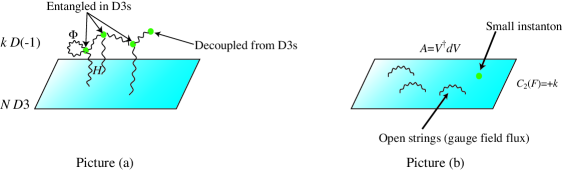
Figure 2: A sketch of a small instanton singularity in our point of view. In the picture (a), some $D(-1)$-branes are decoupled from $D3$-branes. Correspondingly, we can define the gauge transformation only for a part of the Chan-Paton indices entangled in $D3$-branes. Then there are individual $D(-1)$-branes even in the picture (b), which makes the gauge configuration on $D3$-branes diverge.

A small instanton singularity is a conical singularity in the instanton moduli space of k-instantons. Correspondingly, some of the single instantons shrink to zero size, thus, it is not allowed as a regular classical solution of the $4D$ gauge theory. In our view of the ADHM construction as a gauge transformation, this singularity is also understood as follows. For simplicity, let us set $H=0$ in the tachyon profile (4.3). Then, the tachyon profile satisfying the ADHM equation (4.17) gives rise to

$$T^{\dagger}T =u^{2}\mu_{0}\otimes{\mathbf{1}}_{2}=u^{2}|\Phi-{\mathbf{X}}|^{2}\otimes{\mathbf{1}}_{2}.$$ (4.31)

A typical example is a diagonal one $\Phi^{\mu}={\rm diag}(\phi^{\mu}_{1},\cdots,\phi^{\mu}_{k})$. Because $T^{\dagger}T$ have zeros, we cannot apply the gauge transformation of the type (3.3). It is rather better to say that we do not need such a transformation since the tachyon potential is already block diagonal. It leads that, in the $(N+2k)D3$/$2k\overline{D3}$ system, $2k$ pairs of $D3/\overline{D3}$-branes always represents $kD(-1)$-branes while $ND3$-branes is topologically trivial. This means simply that descriptions of $ND3$-branes corresponding to the picture (b) do not exist. A crucial fact here is that for $H=0$ the $ND3$-branes decouple from $2k$ pairs of $D3/\overline{D3}$-branes. Then it is easily generalized for the case with some sub-pairs of $D3/\overline{D3}$-branes decoupled, say $k_{1}$, that corresponds to the matrix $H^{\dagger}H$ has $k_{1}$ zero eigenvalues (see Fig. 2). In that case, we can rotate the Chan-Paton indices for $k_{2}=k-k_{1}$ pairs by the gauge transformation and we have smooth $k_{2}$-instanton on the $ND3$-branes, while $k_{1}\,D(-1)$-branes remain point-like. This is consistent with the understanding in the picture (a) at low energy, where the small instanton singularity is the sign for the connection with the Coulomb branch.

It is instructive to see the zero size limit of the instanton configuration in an explicit example. Let us consider the $N=2$, $k=1$ case [27]. In this case, the tachyon profile satisfying the ADHM equation and the corresponding $\mu_{0}$ are given by

$$T({\mathbf{X}})=u\left(\begin{array}[]{c}\rho\otimes{\mathbf{1}}_{2}\\ (\phi^{\mu}-{\mathbf{X}}^{\mu})\otimes\sigma_{\mu}\end{array}\right),\qquad\mu_{0}=|\phi-{\mathbf{X}}|^{2}+\rho^{2},$$ (4.32)

where $\phi^{\mu}$ and $\rho$ correspond to the position and the size moduli of the instanton, respectively. For $\rho\neq 0$, the gauge transformation in $U(N+2k)$ is well-defined as

$$U_{1}=\frac{1}{\sqrt{\mu_{0}}}\left(\begin{array}[]{cc}(\phi^{\mu}-{\mathbf{X}}^{\mu})\otimes\bar{\sigma}_{\mu}&\rho\otimes{\mathbf{1}}_{2}\\ -\rho\otimes{\mathbf{1}}_{2}&(\phi^{\mu}-{\mathbf{X}}^{\mu})\otimes\sigma_{\mu}\\ \end{array}\right),$$ (4.33)

which gives rise to the BPST instanton solution [27], whose field strength is

$$F_{\mu\nu}=\frac{2i\rho^{2}\eta_{\mu\nu}^{(+)i}\tau_{i}}{(|x-\phi|^{2}+\rho^{2})^{2}}.$$ (4.34)

When the instanton size $\rho$ shrink to zero, (4.34) approaches the $\delta$-function peaked at $x=\phi$. As mentioned above, this limit does not exist because $\mu_{0}$ has zero at a point $x=\phi$. This is seen in the gauge transformation (4.33): it is not unitary so ill-defined at $x=\phi$, and at $x\neq\phi$ it is well-defined but valued in $U(N)\times U(2k)$, which means that $ND3$-branes and $kD(-1)$-branes are decoupled. Therefore, the small instanton is realized only as a $D(-1)$-brane. It is interesting that both of the expressions (4.34) and (4.21) are reminiscent of two expressions of the $\delta$-function,

$$\delta^{(4)}(x-\phi)=\lim_{\rho\rightarrow 0}\frac{\rho^{2}}{(|x-\phi|^{2}+\rho^{2})^{2}}=\lim_{u\rightarrow\infty}\frac{u^{4}}{\pi^{2}}e^{-u^{2}|x-\phi|^{2}}.$$ (4.35)

Although the two parameters $\rho$ and $u$ play the completely different role, it might be interesting to investigate relations between them (see the section 4.5).

4.5 Equivalence beyond BPS

So far, we have assumed that the tachyon profile (4.3) satisfies the ADHM equation (4.17) and showed that the obtained gauge field (3.21) is self-dual (4.25). However, it is apparent from the derivation that, as far as we have kept the assumption that $T^{\dagger}T$ is strictly positive definite, the gauge transformation (3.11) can be defined and (3.21) still gives a non-trivial gauge field configuration on the $ND3$-branes even if one does not assume the ADHM condition. In other words, the equivalence between (a) and (b) holds independent of the BPS condition.

To see what happen if we does not assume the ADHM condition in the picture (a), let us first estimate the field strength on the $ND3$-branes in the picture (b), corresponding to (3.21) without the ADHM condition but assuming $T^{\dagger}T$ is positive definite. Recall that the expression of the field strength (4.24) is applicable to a general tachyon profile. Since $(T^{\dagger}T)^{-1}$ is a $2k\times 2k$ matrix in general, it is expanded with respect to the Pauli matrices $\sigma_{\mu}=(1,-i\tau_{i})$ as

$$(T^{\dagger}T)^{-1}\equiv\sum_{\mu=0}^{3}f_{\mu}\otimes\sigma_{\mu},$$ (4.36)

where $\{{}^{\exists}\!f_{\mu}\}$ is $k\times k$ matrices written by $\{\mu_{0},\,\mu_{i}\}$. Then, since $\partial_{\mu}T$ is unchanged, the field strength can be written as

$$F_{\mu\nu} =\frac{i}{2}\eta_{\mu\nu}^{(+)i}v^{\dagger}\left(f_{0}\otimes\tau_{i}\right)v+\frac{i}{2}\sum_{i=1}^{3}\eta_{\mu\nu}^{(-)i}v^{\dagger}\left(f_{i}\otimes{\mathbf{1}}_{2}\right)v,$$ (4.37)

where we have used the identity,

$$\frac{1}{2}\left(\sigma_{\mu}\sigma_{i}\bar{\sigma}_{\nu}-\sigma_{\nu}\sigma_{i}\bar{\sigma}_{\mu}\right) =i\eta_{\mu\nu}^{(-)i}\,{\mathbf{1}}_{2},\qquad(i=1,2,3)$$ (4.38)

in addition to (4.10). Note that $v$ in (4.37) is different from that given in (4.25) and $f_{0}\neq(\mu_{0})^{-1}$, but of course if we impose the ADHM condition (4.17), it reproduces the self-dual field strength (4.25). In the present case, an anti-self-dual component (the second terms of (4.37)) corresponding to $f_{i}$ is introduced in the field strength. In the low energy Yang-Mills theory, such a deviation from the instanton solution increases the action (mass of the $D3$-branes). From the view point of the string theory, this corresponds to the deviation from the BPS condition, since the RR-charges are preserved even if the tachyon configuration does not satisfy the ADHM condition. Since the ADHM equation is originally the BPS condition for the $kD(-1)$-brane effective theory and its breaking raises the mass, this simply means that the supersymmetry breaking occurs as the same manner in both pictures.

This is a direct consequence of the fact that the picture (a) and (b) are equivalent in the full string theory even if the BPS condition is not satisfied, since it is simply due to the gauge equivalence in the system of $(N+2k)D3$-branes and $2k\overline{D3}$-branes under the gauge symmetry $U(N+2k)\times U(2k)$. We here summarize our claim. The system of $ND3$/$kD(-1)$ bound state in the picture (a) and the system of $ND3$-branes with fluxes in the picture (b) are gauge equivalent with each other. Each picture corresponds to a particular gauge:

$$\text{(a)}\left\{\begin{array}[]{ll}\text{background:}&kD(-1)+ND3\\ \text{fluctuations:}&(H,\Phi^{\mu})\end{array}\right.\,\,\ \text{(b)}\left\{\begin{array}[]{ll}\text{background:}&ND3\\ \text{fluctuations:}&A_{\mu}=-V^{\dagger}\partial_{\mu}V.\end{array}\right.$$

Here the background means a particular boundary state defining a conformal field theory on the disk, and fluctuations are boundary interactions acting on it. The equivalence says that the backgrounds of both pictures are apparently different but the total systems with adding fluctuations are the same. It is because both the background and the fluctuations are determined by the configurations for tachyon and gauge fields (or simply the boundary interaction matrix $\mathbf{M}$) on the $(N+2k)D3$/$2k\overline{D3}$-system. In particular, it gives the correspondence between DN- and DD-strings $\{H,\Phi^{\mu}\}$ in the picture (a) and NN-strings $-V^{\dagger}\partial_{\mu}V$ in the picture (b). This equivalence is quite general in the sense that it is independent of the BPS condition and is valid at all order in $\alpha^{\prime}$. If we additionally impose the BPS condition in both sides, it gives the ADHM construction in the low energy limit. As mentioned, imposing the ADHM condition on $\{H,\Phi^{\mu}\}$ corresponds to restricting the field strength be self-dual. Moreover, the fluctuations $\{H,\Phi^{\mu}\}$ rotated by the $U(k)$ symmetry gives the same $A_{\mu}$, and the gauge transformation itself has ambiguity $U(N)$, which is seen as the (topologically trivial) gauge symmetry in the picture (b). Therefore, we have obtained the map,

$$\frac{\{(H,\Phi^{\mu})|\mbox{ADHM eqs.}\}}{U(k)}\rightarrow\frac{\{-V^{\dagger}\partial_{\mu}V|\mbox{self-dual eqs.}\}}{U(N)}.$$ (4.39)

If we can replace $-V^{\dagger}\partial_{\mu}V$ by an arbitrary gauge field $A_{\mu}$, this map means the isomorphism between the ADHM moduli space and the instanton moduli space.

In the above claim, there is a remaining task to show that $2k$ pairs of $D3$/$\overline{D3}$-branes disappear even if the system is non-BPS. There also arises a natural question, how one can decompose a given field configuration into the background and fluctuations, or whether this decomposition is unique. From the $(N+2k)D3$/$2k\overline{D3}$ point of view it is abuse question and it is a matter of the physical interpretation. It is also related to the definition of the moduli space in the boundary state setting. In the low energy effective theory, in which a background determines the base space (worldvolume) and fluctuations become fields on it, the notion of the moduli space is well-defined. Here let us look at the Fig. 1 again and recall that our argument relies on two independent notions,

1. gauge transformation $U(N+2k)\times U(2k)$,

2. tachyon condensation $u\rightarrow\infty$,

where the first item corresponds to the horizontal line in the Fig. 1 and the second represents two vertical lines. We have so far mainly concentrated ourselves on the first item. In general, any two configurations of the $(N+2k)D3$/$2k\overline{D3}$-system are gauge equivalent with each other as far as there exists a gauge transformation (which is not restricted to a particular form (3.11)) connecting them. On the other hand, our questions are concerned to the second item, so we next discuss the second item in more detail.

Let us examine the boundary interaction in more detail for the tachyon profile (4.3). First, for simplicity, we set $H=0$ in the picture (a), corresponding to small instantons. In this case, $ND3$-branes are decoupled and the boundary interaction $e^{-S_{b}}$ in the NSNS-sector is given as

$$e^{-S_{b}}\left|\,{B3}\,\right\rangle=N\left|\,{B3}\,\right\rangle+e^{-\widetilde{S}_{b}}\left|\,{B3}\,\right\rangle,$$ (4.40)

where the first term is the decoupled $ND3$-branes. We concentrate on the second term, which is $2kD3$/$\overline{D3}$-branes with the boundary interaction given as

$$e^{-\widetilde{S}_{b}}\left|\,{B3}\,\right\rangle ={\rm Tr}_{\!4k}\widehat{P}\exp\left\{\int d\widehat{\sigma}u(\Phi^{\mu}-{\mathbf{X}}^{\mu})\Gamma_{\mu}\right\}\left|\,{B3}\,\right\rangle$$

$$={\rm Tr}_{\!4k}P\exp\left\{\int d\sigma\left(-{u^{2}}|\Phi^{\mu}-X^{\mu}|^{2}{\mathbf{1}}_{4}-{u^{2}}[\Phi^{\mu},\Phi^{\nu}]\Gamma_{\mu\nu}+u\Psi^{\mu}\Gamma_{\mu}\right)\right\}\left|\,{B3}\,\right\rangle$$

$$=\int[d\zeta_{\mu}]\,{{\rm Tr\,}}_{\!k}P\,\,e^{\int d\sigma\left(\frac{1}{4}{\zeta}_{\mu}\partial_{\sigma}{\zeta}_{\mu}-{u^{2}}|\Phi^{\mu}-X^{\mu}|^{2}-{u^{2}}[\Phi^{\mu},\Phi^{\nu}]\zeta_{\mu\nu}+u\Psi^{\mu}\zeta_{\mu}\right)}\left|\,{B3}\,\right\rangle$$

$$=\int[d\zeta_{\mu}][dX_{\mu}][d\Psi_{\mu}]\,{{\rm Tr\,}}_{\!k}P\,\,e^{\int d\sigma\left(\frac{1}{4u^{2}}\zeta_{\mu}\partial_{\sigma}{\zeta}_{\mu}-{u^{2}}|\Phi^{\mu}-X^{\mu}|^{2}-[\Phi^{\mu},\Phi^{\nu}]\zeta_{\mu\nu}+\Psi^{\mu}\zeta_{\mu}\right)}\left|\,{{\mathbf{X}}^{\mu}}\,\right\rangle,$$ (4.41)

where

$$\Gamma_{\mu}\equiv\left(\begin{matrix}0&\sigma_{\mu}\\ \bar{\sigma}_{\mu}&0\end{matrix}\right),$$ (4.42)

is the $4$-dimensional Dirac gamma matrices and $\Gamma_{\mu\nu}\equiv\frac{1}{2}\left[\Gamma_{\mu},\Gamma_{\nu}\right]$. From the second line to the third line, we have replaced $\Gamma_{\mu}$ by the boundary fermions $\zeta_{\mu}(\sigma)$ with the anti-periodic boundary condition and replaced the trace over the Clifford algebra by the functional integral [21]. From the third line to the last line, we have rescaled $\zeta_{\mu}\to\zeta_{\mu}/u$ which does not change the measure $[d\zeta_{\mu}]$ of the anti-periodic boundary fermions. In the language of the decomposition (4.13), the second term of (4.41), $|\Phi^{\mu}-X^{\mu}|^{2}$ is equal to $\mu_{0}$ and the third term, $[\Phi^{\mu},\Phi^{\nu}]\zeta_{\mu\nu}$ is a linear combination of $\mu_{i}$. By performing the functional integral and taking the limit $u\rightarrow\infty$, it reduces to (4.2),

$${\rm Tr}_{k}\,\widehat{P}e^{-i\int d\widehat{\sigma}\Phi^{\mu}\mathbf{P}_{\mu}}\left|\,{{\mathbf{X}}^{\mu}=0}\,\right\rangle={\rm Tr}_{k}\,Pe^{\int d\sigma\left(-i\Phi^{\mu}P_{\mu}-[\Phi^{\mu},\Phi^{\nu}]\Pi_{\mu}\Pi_{\nu}\right)}\left|\,{{\mathbf{X}}^{\mu}=0}\,\right\rangle.$$ (4.43)

The expression (4.41) represents a system (4.43) of $kD(-1)$-brane with scalar fields from the $2kD3$/$\overline{D3}$-branes point of view. Roughly speaking, $\mu_{0}$ ($\mu_{i}$) in (4.41) corresponds to the first (second) term of (4.43). By comparing (4.43) with (4.41), we can read off more precise information on the tachyon condensation. When $\Phi^{\mu}=0$, they represent coincident $kD(-1)$-branes, which define a background $k\left|\,{{\mathbf{X}}^{\mu}=0}\,\right\rangle$ and $\Phi^{\mu}$ are fluctuations around this background. In the low energy effective theory of $kD(-1)$-branes, $\Phi^{\mu}$ become scalar fields on the $0$-dimensional worldvolume, but $\mu_{0}$ and $\mu_{i}$ play the different role. In fact, $\mu_{i}$ term gives rise to the potential term ${\rm Tr\,}_{k}|[\Phi^{\mu},\Phi^{\nu}]|^{2}$ and hence raises the mass, while $\mu_{0}$ term works as the (generalized) pull-back of embedding the worldvolume into the space-time. From the worldsheet point of view, the insertion of $\int d\widehat{\sigma}\Phi^{\mu}\mathbf{P}_{\mu}$ in (4.43) gives a marginal deformation of the disk with the Dirichlet boundary condition, because its conformal dimension is $1$. As far as they are treated perturbatively, such fluctuations do not change the background, but if arbitrary numbers of insertions are allowed and if they are mutually commuting, such marginal perturbation could change the background [28]. For example, if $\Phi^{\mu}={\rm diag.}(\phi^{\mu}_{1},\cdots,\phi^{\mu}_{k})$ are diagonal, $\mu_{i}=0$ and (4.43) becomes

$$\left|\,{X^{\mu}=\phi_{1},\Psi^{\mu}=0}\,\right\rangle+\cdots+\left|\,{X^{\mu}=\phi_{k},\Psi^{\mu}=0}\,\right\rangle,$$ (4.44)

which represents $kD(-1)$-branes located at $x^{\mu}=\phi^{\mu}_{1},\cdots,\phi^{\mu}_{k}$. This is an example of the exactly marginal deformation from coincident $kD(-1)$-branes. Here $4k$ parameters of the location span the moduli space. This means that in terms of (4.41), the principal part of the tachyon condensation is $\mu_{0}$ with $\mu_{i}=0$. Namely, the insertions of $\mu_{0}$ with $\mu_{i}=0$ represent a relevant deformation of the worldsheet, in which the disk with the Neumann boundary condition is deformed to that with the Dirichlet boundary condition, and the possible choice of $\mu_{0}$ span the same moduli space. This is also seen by the $u$-dependence in (4.41): only $\mu_{0}$ contributes to the tachyon condensation $u\rightarrow\infty$, while $\mu_{i}$ are $u$-independent and hence considered to be fluctuations around the condensed background. Physically, it reflects the fact that the $D3$/$\overline{D3}$-system is strongly bounded but the resultant $D(-1)$-branes are marginally bounded with each other.

Some remarks are in order. First, the fact that $\mu_{0}$ has always $k$ zeros at some points (i.e., $T^{\dagger}T$ with $\mu_{i}=0$ has $2k$ zeros), means the resultant defects are small instantons. Second, if we regard whole $T^{\dagger}T$ rather than $\mu_{0}$ as the principal part, or equivalently, if we take the basis diagonalizing $T$ rather than $\mu_{0}$, it never leads to the picture (a) except for the BPS case but leads to another picture, because $\mu_{i}$ terms necessarily split the eigenvalues of $T^{\dagger}T$ and $T^{\dagger}T$ has only $k$ zeros. It also breaks the structure of the fermion $\Psi^{\mu}$ terms, which is also important for defining the background.

The situation is in principle the same when we take into account of $H$. The tachyon profile (2.26) gives $ND3$-branes and $kD(-1)$-branes without open strings, which defines a background in the picture (a). By turning on the massless open strings $\{H,\Phi^{\mu}\}$ as perturbations, they still represent the same system with fluctuations. However, if we include $\{H,\Phi^{\mu}\}$ which satisfy the ADHM equations $\mu_{i}=0$ as background, the condensation of such term represents $ND3$/$kD(-1)$ bound state, which is a exactly marginal deformation from (2.26). All possible choices are equally regarded as the backgrounds for the string theory, that is, they span the moduli space of the $ND3$/$kD(-1)$ bound state. This is the stringy explanation of the ADHM moduli space. On the other hand, $\{H,\Phi^{\mu}\}$ with non-zero $\mu_{i}$ are considered to be fluctuations from this bound state. Therefore, within the picture (a) the decomposition into the background and the fluctuations itself is not unique, but for any choice the total system is the same.

Under the gauge transformation, this structure is mapped to the picture (b). Treating $\mu_{0}$ with $\mu_{i}=0$ as the principal part of the tachyon condensation is the same as taking $P_{0}=\mu_{0}$ in (3.14) in the section 3. It is exactly the ADHM construction argued in the section 4.3. If $\mu_{0}$ is strictly positive definite (no small instantons), $2k$ pairs of $D3$/$\overline{D3}$-branes are always annihilated into the vacuum for any choices of $\mu_{0}$ and a self-dual gauge field appears on the remaining $ND3$-branes. In other words, possible backgrounds of the picture (b) are $ND3$-branes with self-dual field strength, which depends on moduli parameters. On the other hand, the effect of fluctuations are contained not only in $\mu_{i}$ but also in the pure gauge part $\mathbf{A}$ in (3.14), since the gauge transformation is defined not by $\mu_{0}$ but by whole $T$. Note that the fate of $2k$ pairs of $D3$/$\overline{D3}$-branes is unchanged by including the $\mu_{i}$ term because they are treated perturbatively and becomes hidden into the vacuum. Therefore, fluctuations are seen only as the deviations of the gauge field from the instanton solution. This explain the correspondence with the deviation from the ADHM equations in the picture (a), as we demonstrated at the beginning of this subsection.

Along this line, we can further extend our analysis. Other kinds of open string excitations can be incorporated as fluctuations in both sides. An rather trivial example is turning on the transverse scaler fields $\Phi^{i}$ on the $ND3$-branes. In this case, if the system is BPS, they define the new backgrounds with $U(N)$ gauge symmetry breaking as seen from the low energy effective theory. Another example is turning on the scalar fields on the $2k$ pairs of $D3$/$\overline{D3}$-branes, which corresponds to the Coulomb branch in the picture (a). More interesting possibility is an insertion of massive excitations. If the tachyon condensation parameter $u$ is quite large but finite, such a non-infinity effect can be regarded as a massive excitation around the $u=\infty$ background [24], that is, $kD(-1)$-branes in the picture (a). Corresponding boundary state is not completely localized but has a size $\sim 1/u$, or equivalently, it possesses a mixed boundary condition on the disk depending on $u$. Such a system would correspond to a gauge configuration in the picture (b), where the defect has minimal size $\sim 1/u$, analogous to the noncommutative instanton, where the existence of B-field changes the boundary condition and possesses the minimal size $\sim\theta$. In this respect, the equation (4.35) could have another meaning. The mechanism presented in the section 3 is also applicable to the $3$ charge system or more complicated D-brane bound states. For example, when scalar fields $3$ of $\Phi^{\mu}$ satisfy the $SU(2)$ Lie algebra, they couple to the RR $2$-form of constant field strength known as the Myers effect [29], then it is better to think that there are also spherical $D1$-branes as the background. In this case, the background of the pictures of (a) and (b) are no longer good backgrounds and there should be a more suitable background which is achieved by a relevant perturbation from them. In any case, however, it is still true that there are several pictures related among them by the gauge transformation in the $D3$/$\overline{D3}$-system.

5 Generalizations

In the previous section, we have concentrated on the construction of instantons which is the codimension 4 bound state of $D(-1)$-branes within $D3$-branes. One might naively expect that we can repeat completely the same arguments in the previous sections and we should obtain in general the bound states with even codimensions $D(-1)$-$D(2n-1)$ after the tachyon condensation. The equivalence between the $D$-brane bound state and gauge field on $D$-branes is still true as we discussed in the section 4.5. However, the final products would not be stable since the bound states are not BPS and break the supersymmetry generally. Let us see here the case of codimension 2 (vortex) and codimensions greater than 4 in detail.

5.1 2 dimensional vortex

We first consider the codimension 2 case, namely $D(-1)$-$D1$ case as vortices. In this case, we need the system of $(N\!+\!k)D1$-branes and $k\overline{D1}$-branes, and the chiral decomposed gamma matrices are simply $\gamma_{0}=1$ and $\gamma_{1}=i$. So the tachyon field in the picture (a) is a holomorphic function of the complex coordinate $z=x^{0}+ix^{1}$ valued in $(N\!+\!k)\times k$ matrices

$$T(z)=u\left(\begin{array}[]{c}H\\ \Phi-z\end{array}\right),$$ (5.1)

where $\Phi$ is a $k\times k$ hermitian matrix and $H$ is a $N\times k$ matrix.

Using the holomorphy of the tachyon $T(z)$, we easily find the 2d analog of the Osborn’s identity [25, 26],

$${\rm Tr\,}F=\partial\overline{\partial}\log\det T^{\dagger}T,$$ (5.2)

where we defined $F\equiv\epsilon_{\mu\nu}F^{\mu\nu}$. Since $T^{\dagger}T$ behaves asymptotically as $\det T^{\dagger}T\sim u^{2}|z|^{2k}$ in the $|z|\rightarrow\infty$ limit, we obtain the vorticity by

$$\frac{1}{2\pi i}\int d^{2}z\,{\rm Tr\,}F=\frac{k}{2\pi i}\oint\frac{dz}{z}=k.$$ (5.3)

As well-known, the codimension 2 bound state is not stable and the localized (finite size) vortex configuration is impossible to be the BPS state. The energy of the vortex is minimized at the large size limit and the $D(-1)$-brane (vortex) should dissolves in the $D1$-brane. (See Sec. 13.6 in [30], for example.) To see this, it is sufficient to estimate the Yang-Mills energy for $U(1)$ one vortex ($N=k=1$). The tachyon field is given by

$$T(z)=\left(\begin{array}[]{cc}h\\ \varphi-z\end{array}\right),$$ (5.4)

where $\varphi$ and $h$ are complex parameters which represents the position and size moduli of the vortex, respectively. Indeed, from (5.2), we find

$$F=\partial\overline{\partial}\log(|\varphi-z|^{2}+|h|^{2})=\frac{|h|^{2}}{(|\varphi-z|^{2}+|h|^{2})^{2}},$$ (5.5)

whose distribution gives the meanings of the moduli parameters. From this $U(1)$ field strength, we can see

$$\frac{1}{2\pi i}\int d^{2}zF=1,$$ (5.6)

independently of $|h|$ as expected. Contrarily, the Yang-Mills energy,

$$\begin{split}E_{\rm YM}&=\frac{1}{4g_{\rm YM}^{2}}\int d^{2}z\,F^{2}\\ &=\frac{\pi}{12g_{\rm YM}^{2}}\frac{1}{|h|^{2}},\end{split}$$ (5.7)

depends on the size moduli $|h|$ and diverges in the limit of $|h|\rightarrow 0$. This means that the minimum of the energy corresponds to the $|h|\rightarrow\infty$ limit. So the $D(-1)$-brane is not localized on $D1$-brane any longer.

From our viewpoint, it is still true that the $D(-1)$-$D1$ bound state in the picture (a) and $D1$-branes with vortices in the picture (b) are gauge equivalent with each other. However, both pictures have instability as the same manner. It is seen in the picture (a) that DN-strings $H$ have tachyonic modes, while in the picture (b) the same $H$ possesses instability of field strength $F$ as described above. Therefore, in this case, these pictures are not good descriptions. It is not a matter of the gauge equivalence but that of the tachyon condensation in the terminology of the section 4.5. If we are interested in the stable BPS state, we should consider other situation like the presence of B-fields or other massless fields, where there are some stabilization effects. Once we have found such a BPS D-brane system, the gauge equivalence would give the construction of corresponding soliton.

5.2 Instantons in dimension greater than four

We next consider the even codimension greater than $4$ case. As in the codimension $2$ case, $D(-1)$-$D5$ or $D(-1)$-$D7$ bound states are not BPS so that the naive extension of the $4$-dimensional instantons does not hold in the higher dimensional case. However, as opposed to the codimension $2$ case, it is possible to find BPS state within the Yang-Mills theory, that is, no additional fields are needed in the low energy effective theory of the picture (b).

In order to obtain the stable BPS states, we need to impose an extended “self-duality” condition for the gauge field in even dimensions greater than four [31, 32]. The extended “self-dual” conditions are expressed as

$$\frac{1}{2}T_{\mu\nu\rho\sigma}F^{\rho\sigma}=\lambda F_{\mu\nu},$$ (5.8)

where $T_{\mu\nu\rho\sigma}$ is a totally antisymmetric tensor and $\lambda$ is an eigenvalue. If $F_{\mu\nu}$ satisfies the condition (5.8), the e.o.m. $D^{\mu}F_{\mu\nu}=0$ is trivially satisfied due to the Jacobi (Bianchi) identity. This linealization of the e.o.m. strongly suggests that the extended self-dual equation is integrable and the solutions give the BPS bound states. In contrast with the 4 dimensional case, the condition (5.8) can not be invariant under the whole Lorentz group $G=SO(2n)$, but invariant under a subgroup $H\subset G$. Therefore the representation of the 4-form tensor $T_{\mu\nu\rho\sigma}$ must contain a singlet piece under $H$ at least.

In the 6 dimensional case, $T_{\mu\nu\rho\sigma}$ belongs to ${\bf 15}$ of $G=SO(6)$. The non-trivial decomposition which does not reduce the 4 dimensional instanton and contains a singlet piece can be done by choosing a subgroup $H=[SU(3)\times U(1)]/{\mathbb{Z}}_{3}$. Under this $H$, the antisymmetric tensor $T_{\mu\nu\rho\sigma}$ and the field strength $F_{\mu\nu}$, which is also ${\bf 15}$ representation, decompose into

$${\bf 15}={\bf 1}_{0}+({\bf 3}_{2}+\overline{\bf 3}_{-2})+{\bf 8}_{0},$$ (5.9)

where the subscripts stand for the $U(1)$ charges, and the singlet, $({\bf 3}+\overline{\bf 3})$ and octet pieces correspond to the eigenvalues $\lambda=-2,-1,1$, respectively. Similarly, an asymmetric product of the gamma matrices (2.27) decomposes into (5.9) as

$$\Gamma_{[\mu}\Gamma_{\nu]}=\eta^{(-2)}_{\mu\nu}+(\eta^{(-1)a}_{\mu\nu}T_{a}+\eta^{(-1)\overline{a}}_{\mu\nu}T^{\dagger}_{\overline{a}})+\eta^{(+1)i}_{\mu\nu}\hat{T}_{i},$$ (5.10)

where $T_{a}$, $T_{\overline{a}}$ and $\hat{T}_{i}$ ($a,\overline{a}=1,\ldots,3$ and $i=1,\ldots,8$) are the generators in $Spin(6)$ representation and $\eta^{(-2)}_{\mu\nu}$, $\eta^{(-1)a}_{\mu\nu}$, $\eta^{(-1)\overline{a}}_{\mu\nu}$ and $\eta^{(+1)i}_{\mu\nu}$ are extended ’t Hooft tensors, which satisfy

$$\frac{1}{2}{T_{\mu\nu}}^{\rho\sigma}\eta^{(\lambda)}_{\rho\sigma}=\lambda\eta^{(\lambda)}_{\rho\sigma}.$$ (5.11)

Following the same ADHM construction of instanton as the 4 dimensional case, we expect that the field strength is proportional to $\gamma_{[\mu}\gamma_{\nu]}^{\dagger}$ if $T^{\dagger}T$ is proportional to the identity matrix (i.e., commute with any $\gamma_{\mu}$), where $\gamma_{\mu}$ is the chiral parts of $\Gamma_{\mu}$ in (2.27). Unfortunately, however, $\gamma_{[\mu}\gamma_{\nu]}^{\dagger}$ is not proportional to any of $\eta^{(\lambda)}_{\mu\nu}$ in contrast with the 4 dimensional case. This means that a naive construction of the 6 dimensional instanton via the tachyon profile,

$$T({\mathbf{X}})=u\left(\begin{array}[]{c}H\\ (\Phi^{\mu}-{\mathbf{X}}^{\mu})\otimes\gamma_{\mu}\end{array}\right),$$ (5.12)

does not give the self-dual 6 dimensional instanton (5.8). It reflects the fact that the $D(-1)$-$D5$ BPS bound state can not exist without $B$-field [33, 34, 20]. In order to obtain the 6 dimensional instanton configuration, we need more generic tachyon profile which respects for the broken Lorentz symmetry $[SU(3)\times U(1)]/{\mathbb{Z}}_{3}$, but this is out of issue in this paper.

Next, let us see the 8 dimensional case. $T_{\mu\nu\rho\sigma}$ belongs to ${\bf 70}={\bf 35}+\overline{\bf 35}$. There are four possible subgroups $H$ of the Lorentz group $G=SO(8)$, which are $Spin(7)$, $[SU(4)\times U(1)]/{\mathbb{Z}}_{4}$, $[Sp(2)\times Sp(1)]/{\mathbb{Z}}_{2}$ and $SO(4)\times SO(4)$. The $SO(4)\times SO(4)$ case however is rather trivial, since it is an intersection of the 4 dimensional instantons independently. Under the non-trivial subgroups, the field strength $F_{\mu\nu}$ of ${\bf 28}$ is decomposed as

$${\bf 28}={\bf 7}+{\bf 21}, \text{ for }Spin(7),$$ (5.13)

$${\bf 28}={\bf 1}_{0}+({\bf 6}_{2}+{\bf 6}_{-2})+{\bf 15}_{0}, \text{ for }[SU(4)\times U(1)]/{\mathbb{Z}}_{4},$$ (5.14)

$${\bf 28}={\bf 3}+{\bf 15}+{\bf 10}, \text{ for }[Sp(2)\times Sp(1)]/{\mathbb{Z}}_{2}.$$ (5.15)

The strategy to obtain the BPS bound state from the tachyon condensation is the same as the 6 dimensional case. So if we can choose a suitable tachyon profile under the above subgroup, we obtain the ADHM equations and “self-dual” field strength for the 8 dimensional instantons, but it is difficult to construct explicitly, except for the $[Sp(2)\times Sp(1)]/{\mathbb{Z}}_{2}$ case [35, 20]. In the $[Sp(2)\times Sp(1)]/{\mathbb{Z}}_{2}$ case, we can choose the tachyon profile as

$$T({\mathbf{X}})=u\left(\begin{array}[]{cc}I^{\dagger}-K^{\dagger}{\mathbf{Z}}_{4}^{\dagger}-L{\mathbf{Z}}_{3}^{\dagger}&J+K^{\dagger}{\mathbf{Z}}_{3}-L{\mathbf{Z}}_{4}\\ B_{2}^{\dagger}-{\mathbf{Z}}_{2}^{\dagger}-B_{4}^{\dagger}{\mathbf{Z}}_{4}^{\dagger}+B_{3}{\mathbf{Z}}_{3}^{\dagger}&-B_{1}+{\mathbf{Z}}_{1}+B_{4}^{\dagger}{\mathbf{Z}}_{3}+B_{3}{\mathbf{Z}}_{4}\\ B_{1}^{\dagger}-{\mathbf{Z}}_{1}^{\dagger}-B_{3}^{\dagger}{\mathbf{Z}}_{4}^{\dagger}-B_{4}{\mathbf{Z}}_{3}^{\dagger}&B_{2}-{\mathbf{Z}}_{2}+B_{3}^{\dagger}{\mathbf{Z}}_{3}-B_{4}{\mathbf{Z}}_{4}\end{array}\right),$$ (5.16)

where

$${\mathbf{Z}}_{1}\equiv{\mathbf{X}}^{2}+i{\mathbf{X}}^{1},\quad{\mathbf{Z}}_{2}\equiv{\mathbf{X}}^{0}+i{\mathbf{X}}^{3},\quad{\mathbf{Z}}_{3}\equiv{\mathbf{X}}^{6}+i{\mathbf{X}}^{5},\quad{\mathbf{Z}}_{4}\equiv{\mathbf{X}}^{4}+i{\mathbf{X}}^{7},$$ (5.17)

and $k{\times}k$ matrices $B_{i}$ and $N{\times}k$ matrices $(I^{\dagger},J,K^{\dagger},L)$ represents fluctuations. Using this profile, we can repeat the same arguments as the 4 dimensional case and obtain the gauge field strength of ${\bf 3}$ and the ADHM equations of ${\bf 10}$ in (5.15).

We can read off the $D$-brane bound state from the tachyon profile (5.16). Note that this tachyon is a $(N\!+2k)\times 2k$-matrix valued function on the $8$ dimensional worldvolume, that is, the system here is $(N\!+\!2k)D7$/$2k\overline{D7}$-system. Suggested by this, it is regarded as the $D3$-branes within $D7$-branes. Indeed, the profile (5.16) has exactly the same form as (4.3) in the section 4, but the ADHM data are now functions of ${\mathbf{Z}}_{3}$ and ${\mathbf{Z}}_{4}$. For any fixed $({\mathbf{Z}}_{3},{\mathbf{Z}}_{4})$ it represents codimension 4 defects (instantons) localized in the $4$-dimensional $(z_{1},z_{2})$-plane, and its world volume extends along the $4$-dimensional $(z_{3},z_{4})$-plane. It is nothing but the $D3$-branes with the $(z_{3},z_{4})$-dependent fluctuations (ADHM data) in the picture (a). Of course in the picture (b), it represents the family of gauge instantons located in the $(z_{1},z_{2})$-plane, whose moduli are $(z_{3},z_{4})$-dependent. Since the size moduli diverges and the gauge configuration becomes sparse at infinity $|z_{3}|,|z_{4}|\rightarrow\infty$, the energy density is effectively localized in the $8$-dimensional space. We can also see (5.16) as the $(z_{1},z_{2})$-dependent ADHM data, by a suitable change of basis so that (5.16) has the canonical form with respect to ${\mathbf{Z}}_{3}$ and ${\mathbf{Z}}_{4}$. From this viewpoint with fixed $(z_{1},z_{2})$, we can obtain other $D3^{\prime}$-branes, which are localized in the $(z_{3},z_{4})$-plane and extending in the $(z_{1},z_{2})$-plane, with $(z_{1},z_{2})$-dependent fluctuations. So this means that in the picture (a) it represents the intersecting $D3$-branes (instantons) at angles bounded to $D7$-branes [36, 37], whose intersections are non-trivially deformed by the fluctuations.

Finally we comment on interesting dual systems. The breaking of the global Lorentz symmetry is closely related to the number of supercharges preserved by the $D(-1)$-$D(2n-1)$ bound state. If the bound states realize the “self-dual” condition, it preserves some Killing spinors associated with a holonomy group. This fact also says that the BPS bound states are dual to an intersecting brane system or curved space with the same number of the supersymmetry. For example $D(-1)$-$D3$-bound state, we can find the following duality maps:

$$\begin{CD}D(-1)/D3@>{T}>{}>D5/D5^{\prime}@>{S}>{}>NS5/NS5^{\prime}@>{T}>{}>\text{CY${}_{3}$ (conifold)},\end{CD}$$ (5.18)

where $T$ and $S$ stand for T- and S-duality, respectively. The final curved Calabi-Yau 3-fold has $SU(3)$ holonomy, which preserves $1/4$ of supercharges as the same number as the initial $D(-1)$-$D3$ bound state. For other bound state with higher dimensional codimensions, they are dual to 8 dimensional Joyce manifold, Calabi-Yau 4-fold and hyper-Kähler manifold with $Spin(7)$, $SU(4)$ and $Sp(2)$ holonomy, which preserves $1/16$, $1/8$ and $3/16$ of supercharges, respectively. It is interesting to consider the relation between the tachyon condensation and the above special holonomy manifold. It it generally difficult to apply the same dual maps as the above to $D$-$\overline{D}$ system. The dual of the $D$-$\overline{D}$ pair decay however would give a closed tachyon condensation into the curved special holonomy manifolds without $D$-branes but preserving the same number of the supersymmetry.

Appendix A Gauge Transformation of the Boundary Interaction

In this appendix, we prove that the supersymmetric path-ordered product for an $M\!\times\!M$ hermitian matrix $\mathbf{M}(\widehat{\sigma})$,

$$\widehat{W}\equiv{\rm Tr\,}\widehat{P}e^{\int d\widehat{\sigma}\mathbf{M}(\widehat{\sigma})},$$ (A.1)

is invariant under the transformation,

$$\mathbf{M}(\widehat{\sigma})\to\mathbf{M}^{\prime}(\widehat{\sigma})=-U(\widehat{\sigma})^{\dagger}DU(\widehat{\sigma})+U^{\dagger}(\widehat{\sigma})\mathbf{M}(\widehat{\sigma})U(\widehat{\sigma}),$$ (A.2)

for an arbitrary unitary matrix $U\in U(M)$. Here we assume that the matrix $\mathbf{M}(\widehat{\sigma})$ is fermionic and the unitary matrix $U(\widehat{\sigma})$ depends on the supercoordinate as

$$U(\widehat{\sigma})\equiv U_{0}(\sigma)+\theta U_{1}(\sigma),$$ (A.3)

where $U_{0}(\sigma)\in U(M)$ and $U_{1}(\sigma)$ must satisfy

$$U_{0}(\sigma)U_{1}^{\dagger}(\sigma)+U_{1}(\sigma)U_{0}^{\dagger}(\sigma)=0$$ (A.4)

in order to $U(\widehat{\sigma})$ be a unitary matrix. Note that this relation (A.4) is automatically satisfied if the unitary matrix is a function of ${\mathbf{X}}$, $U=U({\mathbf{X}})$, as in the section 2.

In order to show the invariance of $\widehat{W}$ under (A.2), we first write $\mathbf{M}(\widehat{\sigma})$ as

$$\mathbf{M}(\widehat{\sigma})=M_{0}(\sigma)+\theta M_{1}(\sigma).$$ (A.5)

Then we can easily see that $M_{0}$ and $M_{1}$ transform as

$$M_{0} \to M^{\prime}_{0}=U_{0}^{\dagger}M_{0}U_{0}+U_{0}^{\dagger}U_{1},$$ (A.6)

$$M_{1} \to M^{\prime}_{1}=-U_{0}^{\dagger}\partial_{\sigma}U_{0}+U_{0}^{\dagger}M_{1}U_{0}-U_{1}^{\dagger}U_{1}-U_{0}^{\dagger}M_{0}U_{1}+U_{1}^{\dagger}M_{0}U_{0},$$ (A.7)

under the transformation (A.2). In particular, we can show that the combination $M\equiv M_{1}-M_{0}^{2}$ transforms as

$$M\to M^{\prime}=-U_{0}^{\dagger}\partial_{\sigma}U_{0}+U_{0}^{\dagger}MU_{0},$$ (A.8)

using the condition (A.4). Recalling that $\widehat{W}$ can be written in the usual form of Wilson loop as

$$\widehat{W}={\rm Tr\,}Pe^{\int d\sigma M(\sigma)},$$ (A.9)

we can immediately show that $\widehat{W}$ is invariant under the transformation (A.8), which is the gauge transformation for a standard Wilson loop operator. This means that $\widehat{W}$ is invariant under the transformation (A.2).

Appendix B A Formula for the path-ordered product

In this appendix, we evaluate the path-ordered product,

$$T_{A+B}(\sigma_{f},\sigma_{i})\equiv Pe^{\int_{\sigma_{i}}^{\sigma_{f}}d\sigma\left(A(\sigma)+B(\sigma)\right)},$$ (B.1)

with $M\!\times\!M$ matrices $A$ and $B$. From the definition of the path-ordered product, (B.1) can be written as

$$T_{A+B}(\sigma_{f},\sigma_{i})=1+\sum_{n=1}^{\infty}\int d\sigma_{1}\cdots d\sigma_{n} \Bigl{(}A(\sigma_{1})+B(\sigma_{1})\Bigr{)}\cdots\Bigl{(}A(\sigma_{n})+B(\sigma_{n})\Bigr{)}$$

$$\times\theta(\sigma_{f}-\sigma_{n})\theta(\sigma_{n}-\sigma_{n-1})\cdots\theta(\sigma_{1}-\sigma_{i}),$$ (B.2)

where $\theta(\sigma-\sigma^{\prime})$ is the Heaviside step function. Here we take a resummation in (B.2) by gathering terms containing the same number of $B$’s. Clearly, the terms with no $B$ become

$$Pe^{\int_{\sigma_{i}}^{\sigma_{f}}d\sigma A(\sigma)}\Bigl{(}=T_{A}(\sigma_{f},\sigma_{i})\Bigr{)}.$$ (B.3)

Similarly, the summation of the terms with a single $B$ becomes

$$\int d\sigma_{1}\left(Pe^{\int_{\sigma_{1}}^{\sigma_{f}}d\sigma^{\prime}A(\sigma^{\prime})}\right)B(\sigma_{1})\left(Pe^{\int_{\sigma_{i}}^{\sigma_{1}}d\sigma^{\prime}A(\sigma^{\prime})}\right).$$ (B.4)

In general, we can easily see that the summation of the terms with $n$ $B$’s becomes

$$\int d\sigma_{1}\cdots d\sigma_{n}T_{A}(\sigma_{f},\sigma_{n})B(\sigma_{n})T_{A}(\sigma_{n},\sigma_{n-1})B(\sigma_{n-1})\cdots B(\sigma_{1})T_{A}(\sigma_{1},\sigma_{i}).$$ (B.5)

Then we can rewrite (B.1) as

$$T_{A+B}(\sigma_{f},\sigma_{i}) =P_{A}e^{\int_{\sigma_{i}}^{\sigma_{f}}d\sigma B(\sigma)}$$

$$\equiv Pe^{\int_{\sigma_{i}}^{\sigma_{f}}d\sigma A(\sigma)}+\sum_{n=1}^{\infty}\int d\sigma_{1}\cdots d\sigma_{n}T_{A}(\sigma_{f},\sigma_{n})B(\sigma_{n})T_{A}(\sigma_{n},\sigma_{n-1})$$

$$\hskip 199.16928pt\times B(\sigma_{n-1})\cdots B(\sigma_{1})T_{A}(\sigma_{1},\sigma_{i}),$$ (B.6)

where we the symbol $P_{A}$ expresses a kind of path-ordered product with replacing the usual Heaviside step function, $\theta(\sigma-\sigma^{\prime})$, by the “transfer matrix” by $A$, $T_{A}(\sigma-\sigma^{\prime})$.

References

- [1] M. R. Douglas, Branes within branes, hep-th/9512077.
- [2] M. R. Douglas, Gauge Fields and D-branes, J. Geom. Phys. 28 (1998) 255–262 [hep-th/9604198].
- [3] D.-E. Diaconescu, D-branes, monopoles and Nahm equations, Nucl. Phys. B503 (1997) 220–238 [hep-th/9608163].
- [4] E. Witten, Small Instantons in String Theory, Nucl. Phys. B460 (1996) 541–559 [hep-th/9511030].
- [5] M. F. Atiyah, N. J. Hitchin, V. G. Drinfeld and Y. I. Manin, Construction of instantons, Phys. Lett. A65 (1978) 185–187.
- [6] N. Dorey, T. J. Hollowood, V. V. Khoze and M. P. Mattis, The calculus of many instantons, Phys. Rept. 371 (2002) 231–459 [hep-th/0206063].
- [7] E. Corrigan and P. Goddard, CONSTRUCTION OF INSTANTON AND MONOPOLE SOLUTIONS AND RECIPROCITY, Ann. Phys. 154 (1984) 253.
- [8] W. Nahm, A SIMPLE FORMALISM FOR THE BPS MONOPOLE, Phys. Lett. B90 (1980) 413.
- [9] K. Hori, D-branes, T-duality, and index theory, Adv. Theor. Math. Phys. 3 (1999) 281–342 [hep-th/9902102].
- [10] N. Nekrasov and A. Schwarz, Instantons on noncommutative R**4 and (2,0) superconformal six dimensionaltheory, Commun. Math. Phys. 198 (1998) 689–703 [hep-th/9802068].
- [11] M. Billo, M. Frau, I. Pesando, F. Fucito, A. Lerda and A. Liccardo, Classical gauge instantons from open strings, JHEP 02 (2003) 045 [hep-th/0211250].
- [12] M. Billo, M. Frau, S. Sciuto, G. Vallone and A. Lerda, Non-commutative D-instantons, hep-th/0511036.
- [13] A. Sen, Tachyon condensation on the brane antibrane system, JHEP 08 (1998) 012 [hep-th/9805170].
- [14] N. T. Jones, L. Leblond and S. H. H. Tye, Adding a brane to the brane anti-brane action in BSFT, JHEP 10 (2003) 002 [hep-th/0307086].
- [15] A. Ishida, S. Uehara and T. Yada, Tachyon condensation in unbalanced D anti-D system, hep-th/0601050.
- [16] T. Asakawa, S. Sugimoto and S. Terashima, Exact description of D-branes via tachyon condensation, JHEP 02 (2003) 011 [hep-th/0212188].
- [17] E. T. Akhmedov, A. A. Gerasimov and S. L. Shatashvili, On unification of RR couplings, JHEP 07 (2001) 040 [hep-th/0105228].
- [18] K. Hashimoto and S. Terashima, ADHM is tachyon condensation, JHEP 02 (2006) 018 [hep-th/0511297].
- [19] K. Hashimoto and S. Terashima, Stringy derivation of Nahm construction of monopoles, JHEP 09 (2005) 055 [hep-th/0507078].
- [20] K. Ohta, Supersymmetric D-brane bound states with B-field and higher dimensional instantons on noncommutative geometry, Phys. Rev. D64 (2001) 046003 [hep-th/0101082].
- [21] P. Kraus and F. Larsen, Boundary string field theory of the DD-bar system, Phys. Rev. D63 (2001) 106004 [hep-th/0012198].
- [22] T. Takayanagi, S. Terashima and T. Uesugi, Brane-antibrane action from boundary string field theory, JHEP 03 (2001) 019 [hep-th/0012210].
- [23] E. Witten, D-branes and K-theory, JHEP 12 (1998) 019 [hep-th/9810188].
- [24] T. Asakawa, S. Kobayashi and S. Matsuura, Excited D-branes and supergravity solutions, Int. J. Mod. Phys. A21 (2006) 1503–1528 [hep-th/0506221].
- [25] E. Corrigan, P. Goddard, H. Osborn and S. Templeton, ZETA FUNCTION REGULARIZATION] AND MULTI - INSTANTON DETERMINANTS, Nucl. Phys. B159 (1979) 469.
- [26] H. Osborn, CALCULATION OF MULTI-INSTANTON DETERMINANTS, Nucl. Phys. B159 (1979) 497.
- [27] A. A. Belavin, A. M. Polyakov, A. S. Shvarts and Y. S. Tyupkin, Pseudoparticle solutions of the Yang-Mills equations, Phys. Lett. B59 (1975) 85–87.
- [28] A. Recknagel and V. Schomerus, Boundary deformation theory and moduli spaces of D-branes, Nucl. Phys. B545 (1999) 233–282 [hep-th/9811237].
- [29] R. C. Myers, Dielectric-branes, JHEP 12 (1999) 022 [hep-th/9910053].
- [30] J. Polchinski, String theory. Vol. 2: Superstring theory and beyond, . Cambridge, UK: Univ. Pr. (1998) 531 p.
- [31] E. Corrigan, C. Devchand, D. B. Fairlie and J. Nuyts, FIRST ORDER EQUATIONS FOR GAUGE FIELDS IN SPACE OF DIMENSION GREATER THAN FOUR, Nucl. Phys. B214 (1983) 452.
- [32] R. S. Ward, COMPLETELY SOLVABLE GAUGE FIELD EQUATIONS IN DIMENSION GREATER THAN FOUR, Nucl. Phys. B236 (1984) 381.
- [33] M. Mihailescu, I. Y. Park and T. A. Tran, D-branes as solitons of an N = 1, D = 10 non-commutative gauge theory, Phys. Rev. D64 (2001) 046006 [hep-th/0011079].
- [34] E. Witten, BPS bound states of D0-D6 and D0-D8 systems in a B-field, JHEP 04 (2002) 012 [hep-th/0012054].
- [35] E. Corrigan, P. Goddard and A. Kent, SOME COMMENTS ON THE ADHM CONSTRUCTION IN 4k-DIMENSIONS, Commun. Math. Phys. 100 (1985) 1.
- [36] N. Ohta and P. K. Townsend, Supersymmetry of M-branes at angles, Phys. Lett. B418 (1998) 77–84 [hep-th/9710129].
- [37] G. Papadopoulos and A. Teschendorff, Instantons at angles, Phys. Lett. B419 (1998) 115–122 [hep-th/9708116].