Microscopic eigenvalue correlations in QCD with imaginary isospin chemical potential

Abstract

We consider the chiral limit of QCD subjected to an imaginary isospin chemical potential. In the $\epsilon$-regime of the theory we can perform precise analytical calculations based on the zero-momentum Goldstone modes in the low-energy effective theory. We present results for the spectral correlation functions of the associated Dirac operators.

I Introduction

An isospin chemical potential provides a way to “twist” the usual Dirac operator in two different directions. A real isospin chemical potential AKW gives a fermion determinant that is real and positive, and thus amenable to numerical simulations; it does not, however, preserve anti-hermiticity of the Dirac operator itself. An imaginary value of the isospin chemical potential, on the other hand, gives massless Dirac operators that are anti-hermitian; their eigenvalues thus lie on the imaginary axis instead of spreading out into the complex plane. This makes imaginary isospin chemical potential a useful parameter for deformation of the Dirac eigenvalue spectrum.

Recently we have noted DHSS ; DHSST that a particular spectral two-point correlation function of Dirac operator eigenvalues near the origin yields a direct way of determining the pion decay constant, $F_{\pi}$, from lattice gauge theory simulations. An alternative proposal, also using imaginary isospin chemical potential, is to use the distortion of the mass-dependent chiral condensate MT . For the quenched theory it has also been shown that one can use an ordinary (real) baryon chemical potential to extract the pion decay constant from lattice distributions of the Dirac eigenvalues OW ; AB . For gauge group SU(3) and quarks in the fundamental representation, the Dirac operator spectrum with real baryon chemical potential is complex, and the theory with dynamical quarks is difficult to simulate directly due to a complex fermion determinant. For this reason imaginary isospin chemical potential is a more convenient strategy.

For a given non-Abelian gauge potential $A_{\mu}(x)$ we study the two Dirac operators

$$D_{+}\psi_{+}^{(n)}\equiv[\hbox to0.0pt{\raisebox{0.6458pt}{$\mskip 4.0mu/$}\hss}D(A)+i\mu_{\rm iso}\gamma_{0}]\psi_{+}^{(n)}=i\lambda_{+}^{(n)}\psi_{+}^{(n)}$$ (1)

and

$$D_{-}\psi_{-}^{(n)}\equiv[\hbox to0.0pt{\raisebox{0.6458pt}{$\mskip 4.0mu/$}\hss}D(A)-i\mu_{\rm iso}\gamma_{0}]\psi_{-}^{(n)}=i\lambda_{-}^{(n)}\psi_{-}^{(n)},$$ (2)

where $\mu_{\rm iso}$ is real. Both operators $D_{\pm}$ are anti-hermitian, and the eigenvalues $\lambda_{\pm}^{(n)}$ therefore lie on the real line. An imaginary isospin chemical potential can be viewed as an external constant Abelian gauge potential $A_{0}$ that couples to the $u$ and $d$ quark with opposite charges.

Much work has gone into understanding gauge theories at real isospin chemical potential SoS ; KSS ; KT ; STV ; KoS ; Loewe:2002tw ; Barducci:2003un ; Barducci:2004tt , often in terms of the effective low-energy theory. Here we consider the effective theory, a chiral Lagrangian, in the presence of an imaginary isospin chemical potential. With the usual pattern of spontaneous chiral symmetry breaking for two light flavors, the theory is described by a Lie-group valued field $U(x)\in$ SU(2).

Our focus will be on the so-called $\epsilon$-regime of QCD, where the chiral Lagrangian is treated as a perturbative expansion around the zero-momentum modes in a finite volume $V$ LS . Roughly speaking, we are dealing with an expansion in $1/L$ (where $L$ is the linear extent of the finite volume) rather than the usual expansion in a small momentum $p$. There is a well known and intriguing connection between this regime and a universal limit of Random Matrix Theory Jac ; ADMN ; OTV ; DOTV ; TVbeta ; TV1 ; TV , but here we will stay entirely within the framework of the effective chiral Lagrangians.

When the chemical potential is included, the power counting of the $\epsilon$-expansion must be reconsidered. One factorizes the field as $U(x)=U_{0}\exp[i\sqrt{2}\phi(x)/F_{\pi}]$, where $U_{0}$ is the zero momentum part that will be treated exactly, and $\phi(x)$ represents the fluctuation fields (without zero modes). It turns out that the naive guess provides a consistent counting: To leading order one keeps only the static modes in the path integral, while the fluctuation degrees of freedom decouple. This is not completely obvious at first glance, but can be seen as follows. The coupling to the imaginary isospin chemical potential in the chiral Lagrangian is dictated by the way it couples at the quark level [Eqs. (1) and (2)]. Vector sources of that kind give rise to a covariant time derivative in the effective SU(2) Lagrangian KST ; SoS ,

$$\partial_{0}U(x)~{}\rightarrow~{}\nabla_{0}U(x)=\partial_{0}U(x)-i\mu_{\rm iso}[\sigma_{3},U(x)],$$ (3)

where $\sigma_{3}$ is the usual Pauli matrix. The leading-order terms in the effective Lagrangian then read

$${\cal L} = \frac{F_{\pi}}{4}{\rm Tr}\,\left[\nabla_{0}U(x)\nabla_{0}U^{\dagger}(x)+\partial_{i}U(x)\partial_{i}U^{\dagger}(x)\right]$$ (4)

$$-\frac{\Sigma}{2}{\rm Tr}\,\left[{\cal M}U^{\dagger}(x)+{\cal M}^{\dagger}U(x)\right],$$

where ${\cal M}={\rm diag}(m_{u},m_{d})$ is the quark mass matrix and $\Sigma$ is the chiral condensate. When we expand

$$U(x)=U_{0}\left[1+i\sqrt{2}\phi(x)/F_{\pi}+\cdots\right],$$ (5)

this produces the usual kinetic term for $\phi(x)$. Let us recall the power counting in the $\epsilon$-expansion LS : We assume $m_{\pi}\sim p^{2}={\cal O}(\epsilon^{2})$ while $\phi(x)\sim 1/L={\cal O}(\epsilon)$, and a consistent power counting for the $\mu_{\rm iso}$-term is $\mu_{\rm iso}={\cal O}(\epsilon^{2})$. Indeed, when we expand the covariant derivative (3) using Eq. (5) the leading contribution becomes

$$\nabla_{0}U(x)=i\sqrt{2}/F_{\pi}\partial_{0}\phi(x)-i\mu_{\rm iso}[\sigma_{3},U_{0}]+\cdots.$$ (6)

In the chiral Lagrangian (4), the mixed terms $\partial_{0}\phi(x)[\sigma_{3},U_{0}]$ produce only boundary contributions and play no role here. Thus, to leading order in the $\epsilon$-expansion the fluctuation field $\phi(x)$ gives rise only to the kinetic energy term

$$\int\!d^{4}x\,\frac{1}{2}{\rm Tr}\,\partial_{\mu}\phi(x)\partial_{\mu}\phi(x),$$

which decouples as in the theory with $\mu_{\rm iso}=0$.

Collecting the remaining terms we see that the leading contribution to the partition function in the $\epsilon$-regime is the zero-dimensional integral

$${\cal Z}({\cal M};i\mu_{\rm iso})=\int_{SU(2)}dU\,e^{\frac{1}{4}VF_{\pi}^{2}\mu_{\rm iso}^{2}{\rm Tr}\,[U,\sigma_{3}][U^{\dagger},\sigma_{3}]+\frac{1}{2}\Sigma V{\rm Tr}\,({\cal M}^{\dagger}U+{\cal M}U^{\dagger})},$$ (7)

where we have dropped the $0$-suffix on the group element $U\in$ SU(2). Projection onto fixed gauge field topology $\nu$ LS is done by a Fourier transform, and amounts to the simple modification

$${\cal Z}^{\nu}({\cal M};i\mu_{\rm iso})=\int_{U(2)}dU\,(\det U)^{\nu}e^{\frac{1}{4}VF_{\pi}^{2}\mu_{\rm iso}^{2}{\rm Tr}\,[U,\sigma_{3}][U^{\dagger},\sigma_{3}]+\frac{1}{2}\Sigma V{\rm Tr}\,({\cal M}^{\dagger}U+{\cal M}U^{\dagger})}~{}.$$ (8)

One sees that the leading-order contribution to the $\epsilon$-regime depends only on the scaling variables $\hat{m}_{i}\equiv m_{i}\Sigma V$ (where $m_{i}$ are the quark masses) and $\hat{\mu}_{\rm iso}^{2}\equiv\mu_{\rm iso}^{2}F_{\pi}^{2}V$. Both of these scaling variables are of order 1 in the $\epsilon$-counting.

Effective partition functions related to (8), and to its generalizations to more quark flavors of both kinds of statistics, have been studied in great detail recently TV ; SV ; O ; AOSV ; MT ; AFV , and much has been learned about them. A particularly important feature for what follows is that such partition functions satisfy a series of exact relationships relating theories with different numbers of quark flavors to each other. The origin of the formalism lies in the theory of certain integrable systems, but we need here only the identities themselves, which are known under the names of Painlevé and Toda lattice equations K ; SV0 . These equations will be used to provide a non-perturbative definition of a replica limit, which in turn is needed to compute spectral correlation functions of the Dirac operator eigenvalues.

We have organized this paper as follows. In Sec. II we reconsider the case of quenched QCD, for which a comparison with lattice gauge theory simulations has already been presented DHSS . In that paper the analytical results were stated without proof; here we provide the details. The main idea is to focus on a mixed spectral correlation function which is extremely sensitive to imaginary isospin chemical potential. In Sec. III we turn to the physically interesting case of two light quark flavors. The same two-point spectral correlation function is far more difficult to determine analytically. In a previous paper DHSST we briefly reported the final results, and showed how well they compare with lattice gauge theory simulations. The bulk of this paper, including all of Sec. III, is dedicated to the detailed derivation of just those results. Finally, Sec. IV contains our conclusions and an outlook on future work.

II Quenched theory

In order to consider the quenched analogue of the situation outlined in the Introduction we need to define the quenched limit on the effective field theory side. This issue was first resolved in Ref. BG by means of a chiral Lagrangian living on a graded (“supersymmetric”) coset of spontaneous chiral symmetry breaking. An alternative, closer to the approach we shall pursue in this paper, relies on the replica method DS . We stress already here that “quenching,” be it by means of replicas or quark partners of bosonic statistics, is required even in the case of dynamical quarks if one wishes to compute spectral correlation functions of the Dirac operator. Indeed, these methods are the only known approaches that allow access to the low-energy Dirac spectrum from effective field theory.

The result of the quenched calculation was briefly stated in Ref. DHSS , which otherwise focused on the high numerical precision that can be reached for $F_{\pi}$ with the proposed method for measuring it. As a warm-up exercise for the $N_{f}=2$ calculation we will here give the main ingredients behind this quenched result. We stress that the steps we follow are the same for both the quenched and dynamical cases; the only difference is that each step is simpler in the quenched case. We first define a two-point correlation function which is very sensitive to $F_{\pi}$. This correlation function can be obtained from a susceptibility that we define and calculate in the effective theory in the $\epsilon$-regime. This last calculation, performed here using the replica method, is the most difficult part. It requires the use of generating functions that are explicitly derived.

The method of Ref. DHSS is to consider the “mixed” two-point spectral correlation function of the Dirac operators $D_{\pm}$ defined in Eqs. (1) and (2),

$$\rho(\lambda_{+},\lambda_{-};i\mu_{\rm iso})\equiv\left\langle\sum_{n}\delta\left(\lambda_{+}-\lambda_{+}^{(n)}\right)\sum_{m}\delta\left(\lambda_{-}-\lambda_{-}^{(m)}\right)\right\rangle-\left\langle\sum_{n}\delta\left(\lambda_{+}-\lambda_{+}^{(n)}\right)\right\rangle\left\langle\sum_{m}\delta\left(\lambda_{-}-\lambda_{-}^{(m)}\right)\right\rangle,$$ (9)

where the averages are performed over the pure Yang-Mills partition function. In order to reach the $\epsilon$-regime, this correlator is considered in the microscopic limit

$$\rho_{s}(\xi_{+},\xi_{-};i\hat{\mu}_{\rm iso})\equiv\lim_{V\rightarrow\infty}\frac{1}{\Sigma^{2}V^{2}}\rho\left(\frac{\xi_{+}}{\Sigma V},\frac{\xi_{-}}{\Sigma V};\frac{i\hat{\mu}_{\rm iso}}{F_{\pi}\sqrt{V}}\right).$$ (10)

A generating function for the spectral correlation function (9) is the mixed scalar susceptibility,

$$\chi(m_{+},m_{-};i\mu_{\rm iso})\equiv\left\langle{\rm tr}\,\frac{1}{D_{+}+m_{+}}{\rm tr}\,\frac{1}{D_{-}+m_{-}}\right\rangle-\left\langle{\rm tr}\,\frac{1}{D_{+}+m_{+}}\right\rangle\left\langle{\rm tr}\,\frac{1}{D_{-}+m_{-}}\right\rangle.$$ (11)

As above, the averages are performed over the pure Yang-Mills partition function. (Note that this partition function is independent of $m_{+}$ and $m_{-}$.) Written in an eigenvalue representation, Eq. (11) becomes

$$\chi(m_{+},m_{-};i\mu_{\rm iso})=\left\langle\sum_{n}\frac{1}{i\lambda_{+}^{(n)}+m_{+}}\sum_{m}\frac{1}{i\lambda_{-}^{(m)}+m_{-}}\right\rangle-\left\langle\sum_{n}\frac{1}{i\lambda_{+}^{(n)}+m_{+}}\right\rangle\left\langle\sum_{m}\frac{1}{i\lambda_{-}^{(m)}+m_{-}}\right\rangle.$$ (12)

If one knows this function analytically, the spectral two-point function (9) can be computed from the discontinuity across the imaginary axis DOTV ; TV1 ,

$$\rho(\lambda_{+},\lambda_{-};i\mu_{\rm iso}) = \frac{1}{4\pi^{2}}{\rm Disc}[\chi(m_{+},m_{-};\mu_{\rm iso})]_{m_{+}=i\lambda_{+},m_{-}=i\lambda_{-}}$$ (13)

$$= \frac{1}{4\pi^{2}}\lim_{\epsilon\rightarrow 0^{+}}[\chi(i\lambda_{+}+\epsilon,i\lambda_{-}+\epsilon;\mu_{\rm iso})-\chi(i\lambda_{+}-\epsilon,i\lambda_{-}+\epsilon;\mu_{\rm iso})$$

$$\qquad\qquad\quad-\chi(i\lambda_{+}+\epsilon,i\lambda_{-}-\epsilon;\mu_{\rm iso})+\chi(i\lambda_{+}-\epsilon,i\lambda_{-}-\epsilon;\mu_{\rm iso})],$$

which is the inverse of the relation

$$\chi(m_{+},m_{-};i\mu_{\rm iso}) = \int_{-\infty}^{\infty}d\lambda_{+}\,d\lambda_{-}\,\frac{\rho(\lambda_{+},\lambda_{-};i\mu_{\rm iso})}{(i\lambda_{+}+m_{+})(i\lambda_{-}+m_{-})}.$$ (14)

In the replica formalism the mixed scalar susceptibility (11) can be defined as DS

$$\chi(m_{+},m_{-};i\mu_{\rm iso})\equiv\lim_{n\rightarrow 0}\frac{1}{n^{2}}\partial_{m_{+}}\partial_{m_{-}}\log{\cal Z}^{\nu}_{2n}(m_{+},m_{-};i\mu_{\rm iso}),$$ (15)

where ${\cal Z}^{\nu}_{2n}(m_{+},m_{-};i\mu_{\rm iso})$ is the effective partition function of $2n$ replicated quark flavors. Half of these have degenerate masses $m_{+}$ and chemical potential $i\mu_{\rm iso}$, while the remaining $n$ flavors have degenerate masses $m_{-}$ and chemical potential $-i\mu_{\rm iso}$. At the level of the fundamental theory,

$${\cal Z}^{\nu}_{2n}(m_{+},m_{-};i\mu_{\rm iso})=\int[{\rm d}A]_{\nu}\det(D_{+}+m_{+})^{n}\det(D_{-}+m_{-})^{n}e^{-S_{\rm YM}(A)}.$$ (16)

The leading contribution in the $\epsilon$-regime is analogous to the SU(2) case discussed in the introduction, and reads SV

$${\cal Z}^{\nu}_{2n}(\hat{m}_{+},\hat{m}_{-};i\hat{\mu}_{\rm iso})=\int_{U\in U(2n)}dU\,\det(U)^{\nu}e^{\frac{1}{4}\hat{\mu}_{\rm iso}^{2}{\rm Tr}\,[U,B][U^{\dagger},B]+\frac{1}{2}{\rm Tr}\,(M^{\dagger}U+MU^{\dagger})},$$ (17)

where $B={\rm diag}({\mathbf{1}}_{n},-{\mathbf{1}}_{n})$ and $M={\rm diag}(\hat{m}_{+},\ldots,\hat{m}_{+},\hat{m}_{-},\ldots,\hat{m}_{-})$, in terms of the scaling variables

$$\hat{m}_{\pm}\equiv m_{\pm}\Sigma V\ \ \ {\rm and}\ \ \ \hat{\mu}_{\rm iso}\equiv\mu_{\rm iso}F_{\pi}\sqrt{V}.$$ (18)

We also use ${\cal Z}$ to denote the partition function in the $\epsilon$-regime, but to distinguish it from the general partition function (16), we write it explicitly as a function of the scaled variables. Because these partition functions (17) are linked to an integrable structure (of an otherwise unrelated Hamiltonian system), it turns out that all can be derived from just the $n=1$ case footnote ,

$${\cal Z}^{\nu}_{2}(\hat{m}_{+},\hat{m}_{-};i\hat{\mu}_{\rm iso})=e^{-2\hat{\mu}_{\rm iso}^{2}}\int_{0}^{1}dt\,te^{2\hat{\mu}_{\rm iso}^{2}t^{2}}I_{\nu}(t\hat{m}_{+})I_{\nu}(t\hat{m}_{-}),$$ (19)

by means of SV

$${\cal Z}^{\nu}_{2n}(\hat{m}_{+},\hat{m}_{-};i\hat{\mu}_{\rm iso})=\frac{D_{n}}{(\hat{m}_{+}\hat{m}_{-})^{n(n-1)}}\det\left[(\hat{m}_{+}\partial_{\hat{m}_{+}})^{k}(\hat{m}_{-}\partial_{\hat{m}_{-}})^{l}{\cal Z}^{\nu}_{2}(\hat{m}_{+},\hat{m}_{-};i\hat{\mu}_{\rm iso})\right]_{k,l=0,1,\ldots,n-1}.$$ (20)

Here $D_{n}$ is a normalization factor whose exact value need not concern us here. It is chosen so that the effective partition functions (17) satisfy the Toda lattice equation ($D_{n}$ determines the coefficient of proportionality) SV

$$\hat{m}_{+}\partial_{\hat{m}_{+}}\hat{m}_{-}\partial_{\hat{m}_{-}}\log{\cal Z}^{\nu}_{2n}(\hat{m}_{+},\hat{m}_{-};i\hat{\mu}_{\rm iso})=4n^{2}(\hat{m}_{+}\hat{m}_{-})^{2}\frac{{\cal Z}^{\nu}_{2n+2}(\hat{m}_{+},\hat{m}_{-};i\hat{\mu}_{\rm iso}){\cal Z}^{\nu}_{2n-2}(\hat{m}_{+},\hat{m}_{-};i\hat{\mu}_{\rm iso})}{[{\cal Z}^{\nu}_{2n}(\hat{m}_{+},\hat{m}_{-};i\hat{\mu}_{\rm iso})]^{2}}~{}.$$ (21)

Using this exact equation to define the replica limit, we obtain

$$\chi(\hat{m}_{+},\hat{m}_{-};i\hat{\mu}_{\rm iso})=4\hat{m}_{+}\hat{m}_{-}{\cal Z}^{\nu}_{2}(\hat{m}_{+},\hat{m}_{-};i\hat{\mu}_{\rm iso}){\cal Z}^{\nu}_{-2}(\hat{m}_{+},\hat{m}_{-};i\hat{\mu}_{\rm iso})~{}.$$ (22)

Apart from the U(2) partition function (8), now given by (19), we also need ${\cal Z}^{\nu}_{-2}(\hat{m}_{+},\hat{m}_{-};i\hat{\mu}_{\rm iso})$. This is the partition function of $-2$ fermionic quarks, i.e., 2 quarks of bosonic statistics. Like its fermionic analogue, the effective bosonic partition function is determined by the symmetries of the underlying QCD Lagrangian, now with bosonic quarks. In addition, in the bosonic case one must carefully enforce the convergence of the partition function DOTV ; SS , a problem that is absent in the fermionic case due to the nature of Grassmann integration. As the purely imaginary chemical potential does not change the hermiticity properties of the Dirac operator, this does not lead to additional constraints as it does for real chemical potential SV ; AOSV . The bosonic partition function can be written as the integral

$${\cal Z}^{\nu}_{-2}(\hat{m}_{+},\hat{m}_{-};i\hat{\mu}_{\rm iso})=\int\frac{dQ\,\theta(Q)}{{\det}^{2}Q}\det(Q)^{\nu}e^{-\frac{1}{4}\hat{\mu}_{\rm iso}^{2}{\rm tr}\,[Q,B][Q^{-1},B]-\frac{1}{2}{\rm tr}\,({\cal M}^{\dagger}Q+Q^{-1}{\cal M})},$$ (23)

where $dQ\,\theta(Q)/{\det}^{2}Q$ is the integration measure on positive definite Hermitian matrices. Using the parametrization

$$Q=e^{t}\left(\begin{array}[]{cc}e^{r}\cosh s&e^{i\theta}\sinh s\\ e^{-i\theta}\sinh s&e^{-r}\cosh s\end{array}\right),$$ (26)

where

$$r\in[-\infty,\infty],\quad s\in[-\infty,\infty],\quad t\in[-\infty,\infty],\quad\theta\in[0,\pi],$$ (27)

we find

$${\cal Z}^{\nu}_{-2}(\hat{m}_{+},\hat{m}_{-};i\hat{\mu}_{\rm iso})=e^{2\hat{\mu}_{\rm iso}^{2}}\int_{1}^{\infty}dt\,te^{-2\hat{\mu}_{\rm iso}^{2}t^{2}}K_{\nu}(t\hat{m}_{+})K_{\nu}(t\hat{m}_{-}).$$ (28)

At $\hat{\mu}_{\rm iso}=0$ this integral can be done analytically,

$${\cal Z}^{\nu}_{-2}(\hat{m}_{+},\hat{m}_{-};i\hat{\mu}_{\rm iso}=0)=\frac{\hat{m}_{+}K_{\nu+1}(\hat{m}_{+})K_{\nu}(\hat{m}_{-})-\hat{m}_{-}K_{\nu+1}(\hat{m}_{+})K_{\nu}(\hat{m}_{-})}{\hat{m}_{+}^{2}-\hat{m}_{-}^{2}},$$ (29)

and the result agrees with the expression at $\mu_{\rm iso}=0$ that was derived in Refs. DV ; FA . The main difference between this and the corresponding fermionic result is the replacement of modified Bessel functions $I_{n}(x)$ by $K_{n}(x)$. This can be traced back to the non-compact integration range in (23), which in turn follows from the symmetries and convergence requirements of the theory with bosonic quarks.

With the above ingredients we immediately find the mixed scalar susceptibility from Eq. (22),

$$\chi(\hat{m}_{+},\hat{m}_{-};i\hat{\mu}_{\rm iso})=4\hat{m}_{+}\hat{m}_{-}\left[\int_{0}^{1}dt\,te^{2\hat{\mu}_{\rm iso}^{2}t^{2}}I_{\nu}(t\hat{m}_{+})I_{\nu}(t\hat{m}_{-})\right]\left[\int_{1}^{\infty}dt\,te^{-2\hat{\mu}_{\rm iso}^{2}t^{2}}K_{\nu}(t\hat{m}_{+})K_{\nu}(t\hat{m}_{-})\right].$$ (30)

Taking the discontinuity as dictated by Eq. (13), we finally obtain the desired quenched spectral correlation function,

$$\rho_{s}(\xi_{+},\xi_{-};i\hat{\mu}_{\rm iso}) = \xi_{+}\xi_{-}\left[\int_{0}^{1}dt\,te^{2\hat{\mu}_{\rm iso}^{2}t^{2}}J_{\nu}(t\xi_{+})J_{\nu}(t\xi_{-})\right]\left[\int_{1}^{\infty}dt\,te^{-2\hat{\mu}_{\rm iso}^{2}t^{2}}J_{\nu}(t\xi_{+})J_{\nu}(t\xi_{-})\right]$$

$$= \xi_{+}\xi_{-}\left[\int_{0}^{1}dt\,te^{2\hat{\mu}_{\rm iso}^{2}t^{2}}J_{\nu}(t\xi_{+})J_{\nu}(t\xi_{-})\right]$$

$$\times\left[\frac{1}{4\hat{\mu}_{\rm iso}^{2}}\exp\left(-\frac{(\xi_{+}^{2}+\xi_{-}^{2})}{8\hat{\mu}_{\rm iso}^{2}}\right)I_{\nu}\left(\frac{\xi_{+}\xi_{-}}{4\hat{\mu}_{\rm iso}^{2}}\right)-\int_{0}^{1}dt\,te^{-2\hat{\mu}_{\rm iso}^{2}t^{2}}J_{\nu}(t\xi_{+})J_{\nu}(t\xi_{-})\right].$$

In the last line we have traded one non-compact integral for an integral over the compact interval $[0,1]$. This is convenient if one wishes to evaluate the expression numerically.

Again it is useful to check the limiting case $\mu_{\rm iso}=0$, where the above expression can be simplified. Using the orthogonality properties of modified Bessel functions on the interval $[0,\infty]$, we have

$$\int_{1}^{\infty}dt\,tJ_{\nu}(t\xi_{+})J_{\nu}(t\xi_{-}) = \int_{0}^{\infty}dt\,tJ_{\nu}(t\xi_{+})J_{\nu}(t\xi_{-})-\int_{0}^{1}dt\,tJ_{\nu}(t\xi_{+})J_{\nu}(t\xi_{+})$$ (32)

$$= \frac{1}{\xi_{+}}\delta(\xi_{+}-\xi_{-})-\frac{\xi_{+}J_{\nu+1}(\xi_{+})J_{\nu}(\xi_{-})-\xi_{-}J_{\nu+1}(\xi_{-})J_{\nu}(\xi_{+})}{(\xi_{+}^{2}-\xi_{-}^{2})}~{}.$$

This allows us to rewrite the above expression for $\mu_{\rm iso}=0$ as

$$\rho_{s}(\xi_{+},\xi_{-};i\hat{\mu}_{\rm iso}=0) = \delta(\xi_{+}-\xi_{-})\frac{\xi_{+}}{2}[J_{\nu}^{2}(\xi_{+})-J_{\nu+1}(\xi_{+})J_{\nu-1}(\xi_{+})]$$ (34)

$$-\frac{\xi_{+}\xi_{-}}{(\xi_{+}^{2}-\xi_{-}^{2})^{2}}\left[\xi_{+}J_{\nu+1}(\xi_{+})J_{\nu}(\xi_{-})-\xi_{-}J_{\nu+1}(\xi_{-})J_{\nu}(\xi_{+})\right]^{2}.$$

which agrees with the known result Jac ; ADMN ; TV1 . When the two eigenvalues $\xi_{\pm}$ coincide there is an explicit $\delta$-function contribution whose coefficient is given by the spectral one-point function. This is due to eigenvalue auto-correlation. The way that the finite imaginary isospin chemical potential $\mu_{\rm iso}$ “resolves” this $\delta$-function contribution (because the eigenvalues $\xi_{-}$ and $\xi_{+}$ are now associated with two different Dirac operators) is quite spectacular. We show in Fig. 1 the quenched spectral two-point function (II) with one eigenvalue arbitrarily fixed at $\xi_{-}=4$ as a function of the other eigenvalue $\xi_{+}$ for $\hat{\mu}_{\rm iso}^{2}=0$, 0.001, 0.01, and 0.05. The pronounced peak around $\xi_{+}=4$ is precisely the remnant of the $\delta$-function at $\xi_{-}=\xi_{+}$. It has been shown in Ref. DHSS how this spreading out of the $\delta$-function provides a method for determining the pion decay constant $F_{\pi}$ in lattice gauge theory simulations.

Figure 1: The quenched two point-correlation function (II) with one eigenvalue arbitrarily fixed at $\xi_{-}=4$ as a function of the other eigenvalue $\xi_{+}$. The full curves correspond to $\hat{\mu}_{\rm iso}^{2}=0.001$, $0.01$ and $0.05$. The curve with the narrowest peak corresponds to the smallest value of $\hat{\mu}_{\rm iso}$. Also shown (dashed) is the curve for $\hat{\mu}_{\rm iso}=0$ where the peak becomes a $\delta$-function at $\xi_{-}=\xi_{+}=4$. The $\delta$-function has been suppressed from this figure.

III Two light flavors

We now turn to the physically more important problem: QCD with two light flavors. As stated above, we follow the same steps as in the quenched case. We first define the two-point correlation function that is very sensitive to $F_{\pi}$. This correlator can easily be obtained from a susceptibility that we calculate in the $\epsilon$-regime of the low-energy effective theory using the replica method. To perform this calculation, we use a Toda lattice equation which requires the introduction of several generating functions with different numbers of fermionic and bosonic quarks.

We thus consider the correlation function

$$\rho(\lambda_{+},\lambda_{-},m_{u},m_{d};i\mu_{\rm iso})$$ (35)

$$\ \ \equiv\Bigl{\langle}\sum_{n}\delta\left(\lambda_{+}-\lambda_{+}^{(n)}\right)\sum_{m}\delta\left(\lambda_{-}-\lambda_{-}^{(m)}\right)\Bigr{\rangle}$$

$$\ \ \ \ \ \ -\Bigl{\langle}\sum_{n}\delta\left(\lambda_{+}-\lambda_{+}^{(n)}\right)\Bigr{\rangle}\Bigl{\langle}\sum_{m}\delta\left(\lambda_{-}-\lambda_{-}^{(m)}\right)\Bigr{\rangle}$$

between the eigenvalues $\lambda_{+}$ and $\lambda_{-}$ of the anti-hermitian operators $D_{+}$ and $D_{-}$, defined in Eqs. (1) and (2), respectively. The average in (35) is taken over the QCD partition function with two light flavors with masses $m_{u}$ and $m_{d}$, viz.

$$\Bigl{\langle}\cdots\Bigr{\rangle}\equiv\frac{\int[{\rm d}A]_{\nu}\ \cdots\ \det(D_{+}+m_{u})\det(D_{-}+m_{d})e^{-S_{\rm YM}(A)}}{\int[{\rm d}A]_{\nu}\det(D_{+}+m_{u})\det(D_{-}+m_{d})e^{-S_{\rm YM}(A)}}.$$

As in the quenched case, the $\epsilon$-regime is reached by taking the microscopic limit of this correlator,

$$\rho_{s}(\xi_{+},\xi_{-},\hat{m}_{u},\hat{m}_{d};i\hat{\mu}_{\rm iso})\equiv\lim_{V\rightarrow\infty}\frac{1}{\Sigma^{2}V^{2}}\rho\left(\frac{\xi_{+}}{\Sigma V},\frac{\xi_{-}}{\Sigma V},\frac{\hat{m}_{u}}{\Sigma V},\frac{\hat{m}_{d}}{\Sigma V};\frac{i\hat{\mu}_{\rm iso}}{F_{\pi}\sqrt{V}}\right),$$ (36)

where $\hat{m}_{u,d}\equiv m_{u,d}\Sigma V$.

The scalar susceptibility,

$$\chi(m_{+},m_{-},m_{u},m_{d};i\mu_{\rm iso})\equiv\left\langle{\rm tr}\,\frac{1}{D_{+}+m_{+}}{\rm tr}\,\frac{1}{D_{-}+m_{-}}\right\rangle-\left\langle{\rm tr}\,\frac{1}{D_{+}+m_{+}}\right\rangle\left\langle{\rm tr}\,\frac{1}{D_{-}+m_{-}}\right\rangle,$$ (37)

which in terms of the eigenvalues $\lambda_{+}$ and $\lambda_{-}$ can be written as

$$\chi(m_{+},m_{-},m_{u},m_{d};i\mu_{\rm iso})=\left\langle\sum_{n}\frac{1}{i\lambda_{+}^{(n)}+m_{+}}\sum_{m}\frac{1}{i\lambda_{-}^{(m)}+m_{-}}\right\rangle-\left\langle\sum_{n}\frac{1}{i\lambda_{+}^{(n)}+m_{+}}\right\rangle\left\langle\sum_{m}\frac{1}{i\lambda_{-}^{(m)}+m_{-}}\right\rangle,$$ (38)

allows us to calculate the correlation function from the discontinuity across the imaginary axis since the QCD partition function does not depend on $m_{\pm}$:

$$\rho(\lambda_{+},\lambda_{-},m_{u},m_{d};i\mu_{\rm iso}) = \frac{1}{4\pi^{2}}{\rm Disc}[\chi(m_{+},m_{-},m_{u},m_{d};\mu_{\rm iso})]_{m_{+}=i\lambda_{+},m_{-}=i\lambda_{-}}$$ (39)

$$= \frac{1}{4\pi^{2}}\lim_{\epsilon\rightarrow 0^{+}}[\chi(i\lambda_{+}+\epsilon,i\lambda_{-}+\epsilon,m_{u},m_{d};\mu_{\rm iso})-\chi(i\lambda_{+}-\epsilon,i\lambda_{-}+\epsilon,m_{u},m_{d};\mu_{\rm iso})$$

$$\qquad\qquad-\chi(i\lambda_{+}+\epsilon,i\lambda_{-}-\epsilon,m_{u},m_{d};\mu_{\rm iso})+\chi(i\lambda_{+}-\epsilon,i\lambda_{-}-\epsilon,m_{u},m_{d};\mu_{\rm iso})].$$

The inverse of this relation is

$$\chi(m_{+},m_{-},m_{u},m_{d};i\mu_{\rm iso}) = \int_{-\infty}^{\infty}d\lambda_{+}\,d\lambda_{-}\,\frac{\rho(\lambda_{+},\lambda_{-},m_{u},m_{d};i\mu_{\rm iso})}{(i\lambda_{+}+m_{+})(i\lambda_{-}+m_{-})}.$$ (40)

III.1 The susceptibility from the replica limit

In order to obtain the susceptibility we again employ the replica method, writing

$$\chi(m_{+},m_{-},m_{u},m_{d};i\mu_{\rm iso})=\lim_{n\rightarrow 0}\frac{1}{n^{2}}\partial_{m_{+}}\partial_{m_{-}}\log{\cal Z}^{\nu}_{2n,2}(m_{+},m_{-},m_{u},m_{d};i\mu_{\rm iso}).$$ (41)

The generating functions ${\cal Z}^{\nu}_{2n,2}$ have 2$n$ replica flavors in addition to the two flavors of mass $m_{u}$ and $m_{d}$,

$${\cal Z}^{\nu}_{2n,2}(m_{+},m_{-},m_{u},m_{d};i\mu_{\rm iso}) = \int[{\rm d}A]_{\nu}\left[\det(D_{+}+m_{+})\det(D_{-}+m_{-})\right]^{n}$$ (42)

$$\qquad\qquad\times\det(D_{+}+m_{u})\det(D_{-}+m_{d})e^{-S_{\rm YM}(A)}.$$

Note that half of the replica flavors have mass $m_{+}$ and chemical potential $i\mu_{\rm iso}$ while the other half have mass $m_{-}$ and chemical potential $-i\mu_{\rm iso}$.

In the $\epsilon$-regime the leading contributions to the partition functions ${\cal Z}^{\nu}_{2n,2}$ again satisfy Toda lattice equations. To obtain the correct replica limit $n\rightarrow 0$ in Eq. (41) we make use of this Toda lattice equation SV0 :

$$\hat{m}_{+}\partial_{\hat{m}_{+}}\hat{m}_{-}\partial_{\hat{m}_{-}}\log{\cal Z}^{\nu}_{2n,2}(\hat{m}_{+},\hat{m}_{-},\hat{m}_{u},\hat{m}_{d};i\hat{\mu}_{\rm iso})$$ (43)

$$\qquad\qquad\qquad\qquad=4n^{2}(\hat{m}_{+}\hat{m}_{-})^{2}\frac{{\cal Z}^{\nu}_{2n+2,2}(\hat{m}_{+},\hat{m}_{-},\hat{m}_{u},\hat{m}_{d};i\hat{\mu}_{\rm iso}){\cal Z}^{\nu}_{2n-2,2}(\hat{m}_{+},\hat{m}_{-},\hat{m}_{u},\hat{m}_{d};i\hat{\mu}_{\rm iso})}{[{\cal Z}^{\nu}_{2n,2}(\hat{m}_{+},\hat{m}_{-},\hat{m}_{u},\hat{m}_{d};i\hat{\mu}_{\rm iso})]^{2}}.$$

Taking the replica limit we arrive at

$$\chi(\hat{m}_{+},\hat{m}_{-},\hat{m}_{u},\hat{m}_{d};i\hat{\mu}_{\rm iso})=4\hat{m}_{+}\hat{m}_{-}\frac{{\cal Z}^{\nu}_{2,2}(\hat{m}_{+},\hat{m}_{-},\hat{m}_{u},\hat{m}_{d};i\hat{\mu}_{\rm iso}){\cal Z}^{\nu}_{2,-2}(\hat{m}_{u},\hat{m}_{d}|\hat{m}_{+},\hat{m}_{-};i\hat{\mu}_{\rm iso})}{[{\cal Z}^{\nu}_{2}(\hat{m}_{u},\hat{m}_{d};i\mu_{\rm iso})]^{2}},$$ (44)

where ${\cal Z}^{\nu}_{2n,2}$ has been defined in Eq. (42); ${\cal Z}^{\nu}_{2}(\hat{m}_{u},\hat{m}_{d};i\hat{\mu}_{\rm iso})={\cal Z}^{\nu}_{0,2}(\hat{m}_{+},\hat{m}_{-},\hat{m}_{u},\hat{m}_{d};\hat{\mu}_{\rm iso})$ is the partition function with zero replica flavors; and ${\cal Z}^{\nu}_{2,-2}(\hat{m}_{u},\hat{m}_{d}|\hat{m}_{+},\hat{m}_{-};i\hat{\mu}_{\rm iso})={\cal Z}^{\nu}_{-2,2}(\hat{m}_{+},\hat{m}_{-},\hat{m}_{u},\hat{m}_{d};\hat{\mu}_{\rm iso})$.

The discontinuity of $\chi$ across the imaginary $m_{+}$ and $m_{-}$ axes gives the dynamic correlation function,

$$\rho_{s}(\xi_{+},\xi_{-},\hat{m}_{u},\hat{m}_{d};i\hat{\mu}_{\rm iso})=\xi_{+}\xi_{-}\frac{{\cal Z}^{\nu}_{2,2}(i\xi_{+},i\xi_{-},\hat{m}_{u},\hat{m}_{d};i\hat{\mu}_{\rm iso}){\cal Z}^{\nu}_{2,-2}(\hat{m}_{u},\hat{m}_{d}|i\xi_{+},i\xi_{-};i\hat{\mu}_{\rm iso})}{[{\cal Z}^{\nu}_{2}(\hat{m}_{u},\hat{m}_{d};i\hat{\mu}_{\rm iso})]^{2}}.$$ (45)

We therefore need to calculate three different generating functions: two with fermionic quarks only, and one with both fermionic and bosonic quarks.

III.2 Computing the fermionic partition function

In the effective theory in the $\epsilon$-regime, the generating functions with $n\geq 0$ involved in the calculation of the susceptibility are given by

$${\cal Z}^{\nu}_{2n,2}(\hat{m}_{+},\hat{m}_{-},\hat{m}_{u},\hat{m}_{d};i\hat{\mu}_{\rm iso})=\int_{U\in U(2n+2)}dU\,\det(U)^{\nu}e^{\frac{1}{4}\hat{\mu}_{\rm iso}^{2}{\rm Tr}\,[U,B][U^{\dagger},B]+\frac{1}{2}{\rm Tr}\,(M^{\dagger}U+MU^{\dagger})},$$ (46)

with

$$B={\rm diag}({\mathbf{1}}_{n+1},-{\mathbf{1}}_{n+1})\qquad{\rm and}\qquad M={\rm diag}(\hat{m}_{+},...,\hat{m}_{+},\hat{m}_{u},\hat{m}_{-},...,\hat{m}_{-},\hat{m}_{d}).$$ (47)

The partition function ${\cal Z}^{\nu}_{2}(\hat{m}_{u},\hat{m}_{d};i\hat{\mu}_{\rm iso})$ has been calculated in Eq. (19) above. In addition, ${\cal Z}^{\nu}_{2,2}(\hat{m}_{+},\hat{m}_{-},\hat{m}_{u},\hat{m}_{d};i\hat{\mu}_{\rm iso})$ can be obtained from the calculation presented in Ref. AFV by changing the sign of $\hat{\mu}_{\rm iso}^{2}$. We have thus

$${\cal Z}^{\nu}_{2,2}(\hat{m}_{+},\hat{m}_{-},\hat{m}_{u},\hat{m}_{d};i\hat{\mu}_{\rm iso})=\frac{1}{(\hat{m}_{+}^{2}-\hat{m}_{u}^{2})(\hat{m}_{-}^{2}-\hat{m}_{d}^{2})}\left|\begin{array}[]{cc}{\cal Z}^{\nu}_{2}(\hat{m}_{+},\hat{m}_{-};i\hat{\mu}_{\rm iso})&{\cal Z}^{\nu}_{2}(\hat{m}_{+},\hat{m}_{d};i\hat{\mu}_{\rm iso})\\[2.0pt] {\cal Z}^{\nu}_{2}(\hat{m}_{u},\hat{m}_{-};i\hat{\mu}_{\rm iso})&{\cal Z}^{\nu}_{2}(\hat{m}_{u},\hat{m}_{d};i\hat{\mu}_{\rm iso})\end{array}\right|.$$ (50)

III.3 Computing the supersymmetric partition functions

The calculation of ${\cal Z}^{\nu}_{2,-2}(\hat{m}_{u},\hat{m}_{d}|\hat{m}_{+},\hat{m}_{-};i\hat{\mu}_{\rm iso})$ requires us to perform an exact integral over the supergroup $\hat{\rm Gl}(2|2)$ with two fermionic and two bosonic quark flavors. This is a rather lengthy analytical calculation. We start from the effective generating function in the $\epsilon$-regime which is given by

$${\cal Z}^{\nu}_{2,-2}(\hat{m}_{u},\hat{m}_{d}|\hat{m}_{+},\hat{m}_{-};i\hat{\mu}_{\rm iso})=\int_{\hat{\rm Gl}(2|2)}dU\,{\rm Sdet}^{\nu}Ue^{\frac{1}{4}\hat{\mu}_{\rm iso}^{2}{\rm Str}\,[B,U][B,U^{-1}]+\frac{1}{2}{\rm Str}\,{\cal M}(U+U^{-1})},$$ (51)

where $B={\rm diag}(1,1,-1,-1)$, and the mass matrix is given by

$${\cal M}=\left(\begin{array}[]{cc}M_{+}&0\\ 0&M_{-}\end{array}\right),$$ (54)

with $M_{+}={\rm diag}(\hat{m}_{u},\hat{m}_{+})$ and $M_{-}={\rm diag}(\hat{m}_{d},\hat{m}_{-})$ TVmuRealQCD . At $\mu_{\rm iso}=0$, this is the same as the generating function used in TV . Notice that in the complete effective partition function at $\mu_{\rm iso}=0$ there is an invariant operator that contains the term $\partial_{\nu}{\rm Str}\,\ln U={\rm Str}\,U^{-1}\partial_{\nu}U$ OTV ; DOTV . This operator is obviously absent from the zero-momentum part of the partition function. At non-zero $\mu_{\rm iso}$, this operator is also absent from the zero-momentum part of the partition function since TVmuRealQCD ${\rm Str}\,U^{-1}\nabla_{0}U={\rm Str}\,U^{-1}\partial_{0}U$, and $\nabla_{0}U=\partial_{0}U-i\mu_{\rm iso}[B,U]$ . We can understand this from physics as well: The isospin singlet does not couple to isospin chemical potential.

III.3.1 Parameterization of the Goldstone supermanifold

In order to calculate the exact supergroup integral (51), we have to parameterize the Goldstone manifold. We use the same factorizing parameterization as in Ref. TV :

$$U=\left(\begin{array}[]{cc}w_{1}&0\\ 0&w_{2}\end{array}\right)\left(\begin{array}[]{cc}\sqrt{1-w\bar{w}}&w\\ -\bar{w}&\sqrt{1-\bar{w}w}\end{array}\right)\left(\begin{array}[]{cc}w_{1}&0\\ 0&w_{2}\end{array}\right),$$ (55)

where $w_{1,2}\in\hat{\rm Gl}(1|1)$ and $w,\;\bar{w}\in{\rm Gl}(1|1)$. This parameterization leads to rather simple expressions for the integrand of (51):

$${\rm Sdet}U={\rm Sdet}(w_{1}^{2}\;w_{2}^{2}),$$ (56)

$$\frac{1}{2}{\rm Str}\,{\cal M}(U+U^{-1})\equiv{\cal S}_{1}+{\cal S}_{2},$$ (57)

and

$$\frac{1}{4}\hat{\mu}_{\rm iso}^{2}{\rm Str}\,[B,U][B,U^{-1}]\equiv{\cal S}_{\mu},$$ (58)

with

$${\cal S}_{1} = \frac{1}{2}{\rm Str}\,\left[M_{+}\left(w_{1}\sqrt{1-w\bar{w}}\,w_{1}\right.\right.$$ (59)

$$\qquad\quad\left.\left.+w_{1}^{-1}\sqrt{1-w\bar{w}}\,w_{1}^{-1}\right)\right],$$

$${\cal S}_{2} = \frac{1}{2}{\rm Str}\,\left[M_{-}\left(w_{2}\sqrt{1-\bar{w}w}\,w_{2}\right.\right.$$ (60)

$$\qquad\quad\left.\left.+w_{2}^{-1}\sqrt{1-\bar{w}w}\,w_{2}^{-1}\right)\right],$$

and

$${\cal S}_{\mu}=-2\hat{\mu}_{\rm iso}^{2}{\rm Str}\,\left[w\bar{w}\right].$$ (61)

For $w^{2}_{1,2}\in\hat{\rm Gl}(1|1)$, we use the same parameterization as the one used in Ref. DOTV ,

$$w^{2}_{i}=\Lambda_{i}v_{i},$$ (62)

where

$$\Lambda_{i}=\left(\begin{array}[]{cc}e^{i\psi_{i}}&0\\ 0&e^{s_{i}}\end{array}\right)\quad{\rm and}\quad v_{i}=\exp\left(\begin{array}[]{cc}0&\alpha_{i}\\ \beta_{i}&0\end{array}\right),$$ (67)

with $\psi_{i}\in(-\pi,\pi)$ and $s_{i}\in(-\infty,\infty)$; $\alpha_{i}$ and $\beta_{i}$ are Grassmann variables. The main advantage of this parameterization is that its Berezinian is equal to $1$, as was shown in Ref. DOTV . Thus we parameterize the matrices $w_{1,2}\in\hat{\rm Gl}(1|1)$ so that $w_{i}^{2}=\Lambda_{i}v_{i}$, i.e.,

$$w_{i}=\left(\begin{array}[]{cc}(1+\frac{1}{2}c_{i}\alpha_{i}\beta_{i})\;e^{i\psi_{i}/2}&a_{i}\alpha_{i}\\ b_{i}\beta_{i}&(1-\frac{1}{2}d_{i}\alpha_{i}\beta_{i})\;e^{s/2}\end{array}\right),$$ (70)

where

$$a_{i} = \frac{e^{i\psi_{i}}}{e^{i\psi_{i}/2}+e^{s_{i}/2}}$$

$$b_{i} = \frac{e^{s_{i}}}{e^{i\psi_{i}/2}+e^{s_{i}/2}}$$ (71)

$$c_{i} = \frac{1}{2}-\frac{e^{s_{i}}}{(e^{i\psi_{i}/2}+e^{s_{i}/2})^{2}}$$

$$d_{i} = \frac{1}{2}-\frac{e^{i\psi_{i}}}{(e^{i\psi_{i}/2}+e^{s_{i}/2})^{2}}.$$

For $w,\,\bar{w}\in{\rm Gl}(1|1)$ we use the same polar decomposition as in TV :

$$w=vSu^{-1}\quad{\rm and}\quad\bar{w}=u\bar{S}v^{-1},$$ (72)

where $S$ and $\bar{S}$ are $2\times 2$ diagonal supermatrices with commuting elements given by

$$S = {\rm diag}(\sin\theta e^{i\rho},i\sinh\phi e^{i\sigma}),$$ (73)

$$\bar{S} = {\rm diag}(\sin\theta e^{-i\rho},i\sinh\phi e^{-i\sigma}),$$ (74)

with $\theta\in(0,\pi/2)$, $\phi\in(0,\infty)$, and $\rho,\sigma\in(-\pi,\pi)$, while $u,\,v\in U(1|1)/[U(1)\times U(1)]$ are given by TV

$$u=\exp\left(\begin{array}[]{cc}0&\zeta\\ \chi&0\end{array}\right)\quad{\rm and}\quad v=\exp\left(\begin{array}[]{cc}0&\xi\\ \eta&0\end{array}\right).$$ (79)

With these parameterizations, we obtain

$${\rm Sdet}\,U=\prod_{i}e^{i\psi_{i}-s_{i}}.$$ (80)

In addition, the supertraces in Eqs. (59), (60), and (61) are given by

$${\cal S}_{1}=\frac{1}{2}{\rm Str}\,\left[vCv^{-1}\left(w_{1}M_{+}w_{1}+w_{1}^{-1}M_{+}w_{1}^{-1}\right)\right],$$ (81)

$${\cal S}_{2}=\frac{1}{2}{\rm Str}\,\left[uCu^{-1}\left(w_{2}M_{-}w_{2}+w_{2}^{-1}M_{-}w_{2}^{-1}\right)\right],$$ (82)

and

$${\cal S}_{\mu}=2\hat{\mu}_{\rm iso}^{2}{\rm Str}\,C^{2},$$ (83)

where $C=\sqrt{1-S\bar{S}}={\rm diag}(\cos\theta,\cosh\phi)$. The advantage of our parameterization is that the integral over the supergroup $\hat{\rm Gl}(2|2)$ explicitly contains two independent integrals over $\hat{\rm Gl}(1|1)$, which are simpler to compute analytically.

In order to perform the group integral we need to determine the integration measure that corresponds to our parameterization. The parameterization of the Goldstone manifold (55) is of the form

$$U=WTW.$$ (84)

As was shown in Ref. TV , the measure factorizes into a product of one factor that depends only on $W$ and one factor that depends only on $T$,

$$d\mu(U) = w_{1}^{-2}\,dw_{1}^{2}\,w_{2}^{-2}\,dw_{2}^{2}\,T^{-1}\,dT$$ (85)

$$\equiv \mu(w_{1})\,dw_{1}\,\mu(w_{2})\,dw_{2}\,\mu(w,\bar{w})dw\,d\bar{w}.$$

For $w^{2}_{1,2}\in\hat{\rm Gl}(1|1)$, we have used the same parameterization as in Ref. DOTV . In that paper, it was shown that the Berezinian of this change of variables is equal to $1$, and thus that

$$w_{i}^{-2}\,dw_{i}^{2}=d\psi_{i}\,ds_{i}\,d\alpha_{i}\,d\beta_{i}.$$ (86)

We therefore find that

$$\mu(w_{i})\,dw_{i}=ds_{i}\,d\psi_{i}\,d\alpha_{i}\,d\beta_{i}.$$ (87)

Finally, the parameterization we use for $T$ is exactly the same as the one used in Ref. TV . The measure is given by

$$T^{-1}\,dT = \mu(w,\bar{w})\,dw\,d\bar{w}$$

$$= \frac{i\sinh 2\phi\sin 2\theta}{(\cos^{2}\theta-\cosh^{2}\phi)^{2}}d\theta\,d\phi\,d\rho\,d\sigma\,d\zeta\,d\chi\,d\xi\,d\eta.$$

III.3.2 Efetov-Wegner terms

As for any supersymmetric integral, extreme care has to be taken with the singularities that might be introduced through a specific parameterization of the integration supermanifold and the corresponding measure. The singularities of the measure affect the supersymmetric integral through the so called Efetov-Wegner terms. (See for example Refs. GPW ; DOTV for a discussion of Efetov-Wegner terms.) The measure $\mu(w_{i})\,dw_{i}$ does not contain any singularity in the variables $s_{i}$ and $\psi_{i}$, and there are no Efetov-Wegner terms related to our parameterization of $w_{1,2}$. On the other hand, the measure $T^{-1}\,dT=\mu(w,\bar{w})\,dw\,d\bar{w}$ is singular when $\theta=i\phi$. We therefore expect Efetov-Wegner terms in this case. The method used in GPW can be straightforwardly applied to compute the Efetov-Wegner terms related to our parameterization of $T$. With our parameterization, including the Efetov-Wegner terms, we find that the generating function ${\cal Z}^{\nu}_{2,-2}$ is given by

$${\cal Z}^{\nu}_{2,-2}(\hat{m}_{u},\hat{m}_{d}|\hat{m}_{+},\hat{m}_{-};i\hat{\mu}_{\rm iso}) = \frac{1}{(2\pi)^{3}}\lim_{\epsilon\rightarrow 0}\int d\theta\,d\phi\,d\rho\,d\sigma\,d\zeta\,d\chi\,d\xi\,d\eta\,\frac{i\sinh 2\phi\sin 2\theta}{(\cos^{2}\theta-\cosh^{2}\phi)^{2}}$$

$$\hskip 14.22636pt\times\left[\theta(v_{c}-\epsilon)+\delta(v_{c}-\epsilon)v_{n}+\frac{1}{2}\delta^{\prime}(v_{c}-\epsilon)v_{n}^{2}\right]{\cal I}_{1}{\cal I}_{2}e^{\hat{\mu}_{\rm iso}^{2}(\cos^{2}\theta-\cosh^{2}\phi)},$$

where

$$v_{c} = \sin^{2}\theta+\sinh^{2}\phi$$

$$v_{n} = (\sin^{2}\theta-\sinh^{2}\phi)(\zeta\chi+\xi\eta)+2i\sin\theta\sinh\phi\left(e^{i(\rho-\sigma)}\eta\zeta-e^{-i(\rho-\sigma)}\xi\chi\right)$$ (90)

$$+2(\sin^{2}\theta+\sinh^{2}\phi)\zeta\chi\xi\eta$$

$$v_{n}^{2} = 2(\sin^{2}\theta+\sinh^{2}\phi)^{2}\zeta\chi\xi\eta,$$

and

$${\cal I}_{i}=\frac{1}{2\pi}\int_{-\pi}^{\pi}d\psi_{i}\int_{-\infty}^{\infty}ds_{i}\int d\alpha_{i}\,d\beta_{i}\,e^{{\cal S}_{i}+\nu(i\psi_{i}-s_{i})}.$$ (91)

The normalization is chosen so that $Z^{\nu}_{2,-2}(\hat{m}_{u},\hat{m}_{d}|\hat{m}_{u},\hat{m}_{d};i\hat{\mu}_{\rm iso})=1$.

III.3.3 Analytical result for the supersymmetric partition function

We are now in position to explicitly compute the partition function (51). We first compute ${\cal I}_{i}$ given by Eq. (91). The integral over $\alpha_{i}$ and $\beta_{i}$ is readily obtained by expanding $\exp{\cal S}_{i}$ to first order in $\alpha_{i}$ and $\beta_{i}$. We get

$${\cal I}_{1} = {\cal J}(\hat{m}_{u},\hat{m}_{+},\cos\theta,\cosh\phi)+\xi\eta{\cal K}(\hat{m}_{u},\hat{m}_{+},\cos\theta,\cosh\phi),$$

$${\cal I}_{2} = {\cal J}(\hat{m}_{d},\hat{m}_{-},\cos\theta,\cosh\phi)+\zeta\chi{\cal K}(\hat{m}_{d},\hat{m}_{-},\cos\theta,\cosh\phi),$$ (92)

with

$${\cal J}(x,y,t,p) = \frac{1}{16\pi}\int d\psi ds\;e^{tx\cos\psi-py\cosh s}\frac{e^{\nu(i\psi-s)}}{1+\cosh\frac{s-i\psi}{2}}$$

$$\qquad\quad\times\left[2tx\cos\psi+2py\cosh s+py\cosh\frac{3s-i\psi}{2}+(2px-tx-py+2ty)\cosh\frac{s+i\psi}{2}\right.$$

$$\qquad\qquad\quad\left.+tx\cosh\frac{s-3i\psi}{2}\right],$$

and

$${\cal K}(x,y,t,p) = \frac{t-p}{64\pi}\int d\psi ds\;e^{tx\cos\psi-py\cosh s}\;e^{\nu(i\psi-s)}$$

$$\qquad\quad\times\big{[}px^{2}-ty^{2}+x(2\cos\psi+tx\cos 2\psi)+y(2\cosh s-py\cosh 2s)$$

$$\qquad\qquad\quad+2i(t-p)xy\sin\psi\sinh s\big{]}.$$

Hence the partition function (III.3.2) can be written as

$$Z^{\nu}_{2,-2}(\hat{m}_{u},\hat{m}_{d}|\hat{m}_{+},\hat{m}_{-};i\hat{\mu}_{\rm iso}) = \lim_{\epsilon\rightarrow 0}\int_{0}^{1}dt\int_{1}^{\infty}dp\frac{tp}{(t^{2}-p^{2})^{2}}e^{2\hat{\mu}_{\rm iso}^{2}(t^{2}-p^{2})}\theta(p^{2}-t^{2}-\epsilon)$$

$$\qquad\qquad\quad\times{\cal K}(\hat{m}_{u},\hat{m}_{+},t,p){\cal K}(\hat{m}_{d},\hat{m}_{-},t,p)$$

$$+\lim_{\epsilon\rightarrow 0}\int_{0}^{1}du\int_{0}^{\infty}dv\frac{uv}{(u^{2}+v^{2})^{2}}e^{\hat{\mu}_{\rm iso}^{2}(u^{2}+v^{2})}\delta(u^{2}+v^{2}-\epsilon)$$

$$\quad\times\left\{(u^{2}-v^{2})\left[{\cal K}\left(\hat{m}_{u},\hat{m}_{+},\sqrt{1-u^{2}},\sqrt{1+v^{2}}\right){\cal J}\left(\hat{m}_{d},\hat{m}_{-},\sqrt{1-u^{2}},\sqrt{1+v^{2}}\right)\right.\right.$$

$$\left.\qquad\qquad+{\cal J}\left(\hat{m}_{u},\hat{m}_{+},\sqrt{1-u^{2}},\sqrt{1+v^{2}}\right){\cal K}\left(\hat{m}_{d},\hat{m}_{-},\sqrt{1-u^{2}},\sqrt{1+v^{2}}\right)\right]$$

$$\qquad\left.+(u^{2}+v^{2}){\cal J}\left(\hat{m}_{u},\hat{m}_{+},\sqrt{1-u^{2}},\sqrt{1+v^{2}}\right){\cal J}\left(\hat{m}_{d},\hat{m}_{-},\sqrt{1-u^{2}},\sqrt{1+v^{2}}\right)\right\},$$

where $t=\cos\theta$, $p=\cosh\phi$, $u=\sin\theta$, and $v=\sinh\phi$. We can rewrite the second integral as

$$\lim_{\epsilon\rightarrow 0}\int_{0}^{\pi/2}dq\int_{0}^{1/\sin q}dr\,\sin 2q\,e^{-2\hat{\mu}_{\rm iso}^{2}r}\delta(r-\epsilon)\Bigg{\{}(\cos^{2}q-\sin^{2}q)$$ (96)

$$\times\left[{\cal K}\left(\hat{m}_{u},\hat{m}_{+},\sqrt{1+r\cos^{2}q},\sqrt{1-r\sin^{2}q}\right){\cal J}\left(\hat{m}_{d},\hat{m}_{-},\sqrt{1+r\cos^{2}q},\sqrt{1-r\sin^{2}q}\right)\right.$$

$$\quad\left.+{\cal J}\left(\hat{m}_{u},\hat{m}_{+},\sqrt{1+r\cos^{2}q},\sqrt{1-r\sin^{2}q}\right){\cal K}\left(\hat{m}_{d},\hat{m}_{-},\sqrt{1+r\cos^{2}q},\sqrt{1-r\sin^{2}q}\right)\right]$$

$$+{\cal J}\left(\hat{m}_{u},\hat{m}_{+},\sqrt{1+r\cos^{2}q},\sqrt{1-r\sin^{2}q}\right){\cal J}\left(\hat{m}_{d},\hat{m}_{-},\sqrt{1+r\cos^{2}q},\sqrt{1-r\sin^{2}q}\right)\Bigg{\}}$$

$$= {\cal J}(\hat{m}_{u},\hat{m}_{+},1,1){\cal J}(\hat{m}_{d},\hat{m}_{-},1,1),$$

where $u=\sqrt{r}\cos q$ and $v=\sqrt{r}\sin q$. This gives

$${\cal Z}^{\nu}_{2,-2}(\hat{m}_{u},\hat{m}_{d}|\hat{m}_{+},\hat{m}_{-};i\hat{\mu}_{\rm iso}) = \int_{0}^{1}dt\int_{1}^{\infty}dp\,\frac{tp}{(t^{2}-p^{2})^{2}}e^{2\hat{\mu}_{\rm iso}^{2}(t^{2}-p^{2})}{\cal K}(\hat{m}_{u},\hat{m}_{+},t,p){\cal K}(\hat{m}_{d},\hat{m}_{-},t,p)$$ (97)

$$+{\cal J}(\hat{m}_{u},\hat{m}_{+},1,1){\cal J}(\hat{m}_{d},\hat{m}_{-},1,1).$$

Finally, we have to calculate ${\cal J}(x,y,1,1)$ and ${\cal K}(x,y,t,p)$. The result is

$${\cal J}(x,y,1,1)=\frac{1}{2}\left\{x\left[I_{\nu-1}(x)+I_{\nu+1}(x)\right]K_{\nu}(y)+yI_{\nu}(x)\left[K_{\nu-1}(y)+K_{\nu+1}(y)\right]\right\},$$ (98)

and

$${\cal K}(x,y,t,p)=(x^{2}-y^{2})(t^{2}-p^{2})I_{\nu}(tx)K_{\nu}(py).$$ (99)

The partition function can finally be written as

$${\cal Z}^{\nu}_{2,-2}(\hat{m}_{u},\hat{m}_{d}|\hat{m}_{+},\hat{m}_{-};i\hat{\mu}_{\rm iso}) = \left[(\hat{m}_{u})^{2}-(\hat{m}_{+})^{2}\right]\left[(\hat{m}_{d})^{2}-(\hat{m}_{-})^{2}\right]$$

$$\times\int_{0}^{1}dt\,te^{2\hat{\mu}_{\rm iso}^{2}t}\,I_{\nu}(t\hat{m}_{u})I_{\nu}(t\hat{m}_{d})\int_{1}^{\infty}dp\,pe^{-2\hat{\mu}_{\rm iso}^{2}p}\,K_{\nu}(p\hat{m}_{+})K_{\nu}(p\hat{m}_{-})$$

$$+\frac{1}{4}\left\{\hat{m}_{u}\left[I_{\nu-1}(\hat{m}_{u})+I_{\nu+1}(\hat{m}_{u})\right]K_{\nu}(\hat{m}_{+})+\hat{m}_{+}I_{\nu}(\hat{m}_{u})\left[K_{\nu-1}(\hat{m}_{+})+K_{\nu+1}(\hat{m}_{+})\right]\right\}$$

$$\quad\times\left\{\hat{m}_{d}\left[I_{\nu-1}(\hat{m}_{d})+I_{\nu+1}(\hat{m}_{d})\right]K_{\nu}(\hat{m}_{-})+\hat{m}_{-}I_{\nu}(\hat{m}_{d})\left[K_{\nu-1}(\hat{m}_{-})+K_{\nu+1}(\hat{m}_{-})\right]\right\}.$$

This can be written in a more compact notation as [cf. Eqs. (19) and (28)]

$${\cal Z}^{\nu}_{2,-2}(\hat{m}_{u},\hat{m}_{d}|\hat{m}_{+},\hat{m}_{-};i\hat{\mu}_{\rm iso})=\left|\begin{array}[]{cc}(\hat{m}_{u}^{2}-\hat{m}_{+}^{2}){\cal Z}^{\nu}_{2}(\hat{m}_{u},\hat{m}_{d};i\hat{\mu}_{\rm iso})&{\cal Z}^{\nu}_{1,-1}(\hat{m}_{d}|\hat{m}_{-})\\[2.0pt] -{\cal Z}^{\nu}_{1,-1}(\hat{m}_{u}|\hat{m}_{+})&(\hat{m}_{d}^{2}-\hat{m}_{-}^{2}){\cal Z}^{\nu}_{-2}(\hat{m}_{+},\hat{m}_{-};i\hat{\mu}_{\rm iso})\end{array}\right|,$$ (103)

where the $\mu_{\rm iso}$-independent graded partition function,

$${\cal Z}^{\nu}_{1,-1}(\hat{m}_{u}|\hat{m}_{+})=\frac{1}{2}\left\{\hat{m}_{u}\left[I_{\nu-1}(\hat{m}_{u})+I_{\nu+1}(\hat{m}_{u})\right]K_{\nu}(\hat{m}_{+})+\hat{m}_{+}I_{\nu}(\hat{m}_{u})\left[K_{\nu-1}(\hat{m}_{+})+K_{\nu+1}(\hat{m}_{+})\right]\right\},$$ (104)

was calculated in Ref. DOTV .

Note that ${\cal Z}^{\nu}_{2,-2}(\hat{m}_{+},\hat{m}_{-}|\hat{m}_{+},\hat{m}_{-};i\hat{\mu}_{\rm iso})=1$ as it should. Furthermore, upon expanding ${\cal Z}^{\nu}_{2,-2}(\hat{m}_{u},\hat{m}_{d}|\hat{m}_{+},\hat{m}_{-};i\hat{\mu}_{\rm iso})$ to leading order in $m_{u}-m_{+}$ and $m_{d}-m_{-}$, the quenched correlation function (II) is recovered using the supersymmetric method.

III.4 Final result

We can thus finally compute the two-point correlation function (45), using the analytically calculated generating functions (19), (50), and (103). The result is

$$\rho_{s}(\xi_{+},\xi_{-},\hat{m}_{u},\hat{m}_{d};i\hat{\mu}_{\rm iso}) = \xi_{+}\xi_{-}\left[\int_{0}^{1}dt\;t\;e^{2\hat{\mu}_{\rm iso}^{2}t^{2}}I_{\nu}(t\;\hat{m}_{u})I_{\nu}(t\;\hat{m}_{d})\right]^{-2}$$

$$\times\left(\int_{0}^{1}dt\;t\;e^{2\hat{\mu}_{\rm iso}^{2}t^{2}}J_{\nu}(t\;\xi_{+})J_{\nu}(t\;\xi_{-})\int_{0}^{1}dt\;t\;e^{2\hat{\mu}_{\rm iso}^{2}t^{2}}I_{\nu}(t\;\hat{m}_{u})I_{\nu}(t\;\hat{m}_{d})\right.$$

$$-\left.\int_{0}^{1}dt\;t\;e^{2\hat{\mu}_{\rm iso}^{2}t^{2}}I_{\nu}(t\;\hat{m}_{u})J_{\nu}(t\;\xi_{-})\int_{0}^{1}dt\;t\;e^{2\hat{\mu}_{\rm iso}^{2}t^{2}}J_{\nu}(t\;\xi_{+})I_{\nu}(t\;\hat{m}_{d})\right)$$

$$\times\left(\int_{0}^{1}dt\;t\;e^{2\hat{\mu}_{\rm iso}^{2}t^{2}}I_{\nu}(t\;\hat{m}_{u})I_{\nu}(t\;\hat{m}_{d})\int_{1}^{\infty}dt\;t\;e^{-2\hat{\mu}_{\rm iso}^{2}t^{2}}J_{\nu}(t\;\xi_{+})J_{\nu}(t\;\xi_{-})\right.$$

$$\left.+\frac{(\hat{m}_{u}I_{\nu+1}(\hat{m}_{u})J_{\nu}(\xi_{+})+\xi_{+}J_{\nu+1}(\xi_{+})I_{\nu}(\hat{m}_{u}))(\hat{m}_{d}I_{\nu+1}(\hat{m}_{d})J_{\nu}(\xi_{-})+\xi_{-}J_{\nu+1}(\xi_{-})I_{\nu}(\hat{m}_{d}))}{(\xi_{+}^{2}+\hat{m}_{u}^{2})(\xi_{-}^{2}+\hat{m}_{d}^{2})}\right).$$

For a numerical evaluation it is advantageous to rewrite the non-compact integral appearing in the fourth line as in Eq. (II).

We have performed various checks on this result. For example, at $\hat{\mu}_{\rm iso}=0$ it correctly reduces to the two-point microscopic correlation functions at zero chemical potential OTV ; DOTV . We have also verified that it reduces to the quenched result (II) in the limit where both $m_{u}$ and $m_{d}$ are sent to infinity, as is required by decoupling.

As in the quenched case the correlation function at $\mu_{\rm iso}=0$ has a $\delta$-function at equal arguments. When $\mu_{\rm iso}$ is nonzero this $\delta$-function becomes a peak in the correlation function around equal arguments, as shown in Fig. 2.

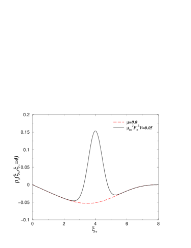
Figure 2: The two-point correlation function (III.4), with one eigenvalue fixed at $\xi_{-}=4$, as a function of the other eigenvalue $\xi_{+}$. The masses of the two dynamical flavors are chosen to be degenerate at the value $\hat{m}_{u}=\hat{m}_{d}=5$. The dashed curve shows the correlation function for $\mu_{\rm iso}=0$ and the solid curve corresponds to $\mu_{\rm iso}^{2}F_{\pi}^{2}V=0.05$. The $\delta$-function that appears at $\xi_{+}=\xi_{-}=4$ when $\mu_{\rm iso}=0$ has been suppressed from this figure.

IV Conclusion

We have considered QCD at nonzero imaginary isospin chemical potential and made use of its effective field theory representation to calculate a correlation function between eigenvalues of the Dirac operator that is very sensitive to the value of the pion decay constant $F_{\pi}$. We have shown the calculation in the quenched case as well as in the physical case with two dynamical light quark flavors. In two previous articles, it has been demonstrated that these formulas for the correlation functions lead to an efficient way to determine $F_{\pi}$ on the lattice DHSS ; DHSST .

Our calculation made extensive use of the replica method. In this approach, the correct answer is reached via Toda lattice equations, which relate theories with differing numbers of quark species to each other. Taking the replica limit required the computation of several partition functions with varying numbers of bosonic and fermionic quarks, which led us to compute some non-trivial partition functions. Our strategy thus required the calculation of exact group integrals over both graded and non-graded Goldstone manifolds. It must be noted that our calculation would be technically very tedious if it were carried out exclusively by the so-called supersymmetric approach: It would require an integration over $\hat{\rm Gl}(4|2)$, a highly complicated task. The advantage of the Toda lattice equation is that it reduces the complexity of the calculation by spreading the difficulty over several partition functions.

As a tool to extract $F_{\pi}$ from dynamical lattice simulations it is of obvious interest to derive the correlation function in a partially quenched theory where the chemical potential is set to zero for the physical dynamical quarks. This would allow the use of existing gauge field ensembles, generated at zero chemical potential, in a determination of $F_{\pi}$. The analytical expression for this partially quenched correlation function has proved to be challenging. We hope that the detailed calculation presented here may be of help in the future calculation of such quantities.

References

(1)
M. G. Alford, A. Kapustin and F. Wilczek,
Phys. Rev. D 59, 054502 (1999)
[hep-lat/9807039].
(2)
P. H. Damgaard, U. M. Heller, K. Splittorff and B. Svetitsky,
Phys. Rev. D 72, 091501 (2005)
[hep-lat/0508029].
(3)
P. H. Damgaard, U. M. Heller, K. Splittorff, B. Svetitsky and D. Toublan,
hep-lat/0602030.
(4)T. Mehen and B. C. Tiburzi,
Phys. Rev. D 72, 014501 (2005)
[hep-lat/0505014].
(5)
J. C. Osborn and T. Wettig,
PoS LAT2005, 200 (2005)
[hep-lat/0510115].
(6)
G. Akemann and E. Bittner,
hep-lat/0603004.
(7)
D. T. Son and M. A. Stephanov,
Phys. Rev. Lett. 86, 592 (2001)
[hep-ph/0005225].
(8)
K. Splittorff, D. T. Son and M. A. Stephanov,
Phys. Rev. D 64, 016003 (2001)
[hep-ph/0012274].
(9)
J. B. Kogut and D. Toublan,
Phys. Rev. D 64, 034007 (2001)
[hep-ph/0103271].
(10)
K. Splittorff, D. Toublan and J. J. M. Verbaarschot,
Nucl. Phys. B 639, 524 (2002)
[hep-ph/0204076].
(11)
J. B. Kogut and D. K. Sinclair,
Phys. Rev. D 66, 034505 (2002)
[hep-lat/0202028];
Phys. Rev. D 70, 094501 (2004)
[hep-lat/0407027].
(12)
A. Barducci, G. Pettini, L. Ravagli and R. Casalbuoni,
Phys. Lett. B 564, 217 (2003)
[hep-ph/0304019].
(13)
A. Barducci, R. Casalbuoni, G. Pettini and L. Ravagli,
Phys. Rev. D 69, 096004 (2004)
[hep-ph/0402104].
(14)
M. Loewe and C. Villavicencio,
Phys. Rev. D 67, 074034 (2003)
[hep-ph/0212275].
(15)J. Gasser and H. Leutwyler,
Phys. Lett. B 184, 83 (1987);
Phys. Lett. B 188, 477 (1987);
H. Neuberger,
Phys. Rev. Lett. 60, 889 (1988);
H. Leutwyler and A. Smilga,
Phys. Rev. D 46, 5607 (1992).
(16)E. V. Shuryak and J. J. M. Verbaarschot,
Nucl. Phys. A 560, 306 (1993)
[hep-th/9212088];
J. J. M. Verbaarschot and I. Zahed,
Phys. Rev. Lett. 70, 3852 (1993)
[hep-th/9303012];
J. J. M. Verbaarschot,
Phys. Rev. Lett. 72, 2531 (1994);
[hep-th/9401059];
(17)
G. Akemann, P. H. Damgaard, U. Magnea and S. Nishigaki,
Nucl. Phys. B 487, 721 (1997)
[hep-th/9609174];
P. H. Damgaard and S. M. Nishigaki,
Nucl. Phys. B 518 (1998) 495
[hep-th/9711023].
(18)
J. C. Osborn, D. Toublan and J. J. M. Verbaarschot,
Nucl. Phys. B 540, 317 (1999)
[hep-th/9806110].
(19)
P. H. Damgaard, J. C. Osborn, D. Toublan and J. J. M. Verbaarschot,
Nucl. Phys. B 547, 305 (1999)
[hep-th/9811212].
(20)
D. Toublan and J. J. M. Verbaarschot,
Nucl. Phys. B 603 (2001) 343
[hep-th/0012144].
(21)
D. Toublan and J. J. M. Verbaarschot,
Nucl. Phys. B 560, 259 (1999)
[hep-th/9904199].
(22)
D. Toublan and J. J. M. Verbaarschot,
Int. J. Mod. Phys. B 15, 1404 (2001)
[hep-th/0001110].
(23)
J. B. Kogut, M. A. Stephanov and D. Toublan,
Phys. Lett. B 464, 183 (1999)
[hep-ph/9906346].
; J. B. Kogut, M. A. Stephanov, D. Toublan, J. J. M. Verbaarschot and A. Zhitnitsky,
Nucl. Phys. B 582, 477 (2000)
[hep-ph/0001171].
(24)
G. Akemann, Y. V. Fyodorov and G. Vernizzi,
Nucl. Phys. B 694 (2004) 59
[hep-th/0404063].
(25)
K. Splittorff and J. J. M. Verbaarschot,
Nucl. Phys. B 683, 467 (2004)
[hep-th/0310271].
(26)
J. C. Osborn,
Phys. Rev. Lett. 93, 222001 (2004)
[hep-th/0403131].
(27)
G. Akemann, J. C. Osborn, K. Splittorff and J. J. M. Verbaarschot,
Nucl. Phys. B 712 (2005) 287
[hep-th/0411030];
J. C. Osborn, K. Splittorff and J. J. M. Verbaarschot,
Phys. Rev. Lett. 94, 202001 (2005)
[hep-th/0501210].
(28)
E. Kanzieper,
Phys. Rev. Lett. 89, 250201 (2002)
[cond-mat/0207745].
(29)
K. Splittorff and J. J. M. Verbaarschot,
Phys. Rev. Lett. 90, 041601 (2003)
[cond-mat/0209594];
Nucl. Phys. B 695, 84 (2004)
[hep-th/0402177].
(30)
C. W. Bernard and M. F. L. Golterman,
Phys. Rev. D 46, 853 (1992)
[hep-lat/9204007].
(31)
P. H. Damgaard and K. Splittorff,
Phys. Rev. D 62, 054509 (2000)
[hep-lat/0003017].
(32)
Note that in order to obtain this result (and other results below) from
calculations based on real baryon chemical potential we make
use of the fact that these involve conjugated quarks as well. In our
present context we re-interpret the conjugated quarks as isospin partners
to the original quarks, and then perform an analytic continuation to
imaginary chemical potential.
(33)
S. R. Sharpe and N. Shoresh,
Phys. Rev. D 64, 114510 (2001)
[hep-lat/0108003];
M. Golterman, S. R. Sharpe and R. L. Singleton,
Phys. Rev. D 71, 094503 (2005)
[hep-lat/0501015].
(34)
D. Dalmazi and J. J. M. Verbaarschot,
Nucl. Phys. B 592, 419 (2001)
[hep-th/0005229].
(35)
Y. V. Fyodorov and G. Akemann,
JETP Lett. 77, 438 (2003)
[Pisma Zh. Eksp. Teor. Fiz. 77, 513 (2003)]
[cond-mat/0210647].
(36)
D. Toublan and J. J. M. Verbaarschot,
arXiv:hep-th/0208021.
(37)
P.-B. Gossiaux, Z. Pluhar, and H.A. Weidenmüller,
Ann. Phys. (N.Y.) 268 (1998) 273 [cond-mat/9803362].