Simple fixed-brane gauges in $S_{1}/\mathbb{Z}_{2}$ braneworlds

Abstract

For five-dimensional braneworlds with an $S_{1}/\mathbb{Z}_{2}$ orbifold topology for the extra dimension $x^{5}$, we discuss the validity of recent claims that a gauge exists where the two boundary branes lie at fixed positions and the metric satisfies $g_{\mu 5}=\partial_{5}g_{55}=0$ where $\mu$ labels the transverse dimensions. We focus on models where the bulk is empty apart from a negative cosmological constant, which, in the case of cosmological symmetry, implies the existence of a static frame with Schwarzschild-AdS geometry. Considering the background case with the branes moving apart after a collision, we show that such a gauge can be constructed perturbatively, expanding in either the time after collision or the brane velocity. Finally we examine how cosmological perturbations can be accommodated in such a gauge.

I Introduction

The large number of recent publications on braneworld cosmology is a testament to the richness and difficulty of this comparatively new field (see, for example, Brax:2004xh ; Langlois:2002bb ; Binetruy:1999ut ; Binetruy:2001tc ; Kim:2003pc ; Maartens:2003tw ). Despite the large gap in complexity between possible String/M-Theory realisations and the greatly simplified models currently being investigated, even the simplest models are extremely rich in new physics. Many such five-dimensional toy models Randall:1999ee ; Lukas:1998tt ; Lukas:1998qs ; Lukas:1999yn ; Shiromizu:2004ig ; Kobayashi:2002pw ; Brax:2000xk ; Brax:2002nt are motivated by the dimensional reduction of Hořava-Witten M-theory Horava:1996ma to five dimensions but miss out most of the resulting large number of bulk degrees of freedom.The extra dimension is assumed to have the topology of an $S_{1}/\mathbb{Z}_{2}$ orbifold, with two 3-branes residing at the boundaries of the spacetime at the two fixed points.

The increase in complexity from a purely four-dimensional Universe to one confined to a brane embedded in a five-dimensional bulk is considerable. We shall therefore mainly focus on the Randall-Sundrum model Randall:1999ee , where the bulk is empty apart from a cosmological constant. We assume that the branes contain no matter and carry equal and opposite tensions finely tuned with respect to the bulk cosmological constant such that their induced cosmological constants vanish, although the conclusions of this paper will not depend sensitively on these assumptions. In the background case, where the transverse dimensions are assumed to possess cosmological symmetry, the lack of non-gravitational degrees of freedom in the bulk then implies the existence of a Birkhoff frame in which the bulk is manifestly static with Anti-de-Sitter(AdS)-Schwarzschild geometry, parameterised by $C$ (related to the black hole mass) and the lengthscale $L$. The velocities of the branes are then determined entirely by their positions, and the system can be solved exactly even in the presence of matter on the branes; the only deviation from four-dimensional Einstein gravity is the presence in the Friedmann equation of quadratic terms in the brane stress-energy and a dark radiation term proportional to $C$, which contains all of the gravitational effects of the bulk.

When one comes to include cosmological perturbations vandeBruck:2000ju ; Maartens:2004yc , however, the problem rapidly becomes intractable, largely due to the considerable increase in number of the gravitational degrees of freedom in going from four to five dimensions. To achieve any sort of analytic result on the propagation of braneworld perturbations one needs to resort to approximations. The simplest is to work to lowest order in the brane velocities, assuming also that the energy content of the branes is much less than their tensions. The result is a four-dimensional effective scalar-tensor theory Mendes:2000wu ; Khoury:2002jq ; Shiromizu:2002qr ; Kanno:2002ia ; Kanno:2002ia2 ; Brax:2002nt ; Webster:2004sp ; Palma:2004et , valid at low energies, formulated for example in terms of the induced metric of one of the branes. The scalar degree of freedom, known as the radion, corresponds to the distance between the two branes.

Attempting to go beyond the very limiting low-energy approximation requires a method of solving the five-dimensional Einstein equations. While a great deal of progress has been made recently Palma:2004fh ; deRham:2004yt ; Calcagni:2003sg ; McFadden:2005mq ; Maartens:1999hf ; Langlois:2000ns ; Liddle:2001yq ; Koyama:2004ap ; deRham:2005qg ; deRham:2005xv ; Shiromizu:2002ve , the problem is still very difficult. The five-dimensional analysis is rendered simpler by choosing a gauge in which the branes are located at fixed positions. The further assumptions that the coordinate $x^{5}$ parameterising the extra dimension is chosen such that both the cross terms $g_{5\mu}$ (where $\mu=0,1,2,3$ labels the transverse time and space dimensions) vanish and $\partial_{5}g_{55}=0$ result in a particularly useful gauge, henceforth referred to as a simple fixed-brane (SFB) gauge. Several publications Kanno:2002ia2 ; deRham:2005qg ; deRham:2005xv ; Shiromizu:2002ve have already assumed, without proof, the existence of SFB gauges to derive effective theories with different, more useful regimes of validity than the low-energy scalar-tensor theory. In particular they focused on the small-radion limit pertinent to recent attempts to model the Big Bang as a brane collision Khoury:2001wf ; Khoury:2001bz ; Gibbons:2005rt ; Jones:2002cv ; Turok:2004gb ; Tolley:2003nx ; Steinhardt:2002ih ; Kanno:2002py .

This paper is organised as follows. In §II we discuss the general problem of constructing SFB gauges, specialising in §III to the special case of background spacetimes with cosmological symmetry. For the case of two branes moving apart after a collision, initially considered in the Birkhoff frame, we construct in §IV the required coordinate transformation as a power series in the SFB time $t$, equivalent to an expansion in the radion. We show that such a gauge can be found correct to arbitrary orders in $t$, although there is in general no analytic expression for the terms in the series and one must resort to numerical methods. We also comment on the convergence of this series and its relation to the horizon structure of the bulk. A second method is derived in §V, namely an expansion in $\sqrt{C}$, which is equivalent to the velocity of the branes. This turns out to be simpler, with analytic expressions available at all orders. Finally we discuss cosmological perturbations in §VI, and show the existence of the gauge transformations which will accommodate general perturbations into an SFB gauge.

II General Formalism

We take our spacetime to be an $S_{1}/\mathbb{Z}_{2}$ orbifold with two boundary branes at the fixed points. We assume first of all the existence of a Gaussian-Normal coordinate system relative to the positive tension brane at $\tilde{y}=0$, with metric

$$\mathrm{d}s^{2}=\mathrm{d}\tilde{y}^{2}+h_{\mu\nu}\left(\tilde{x},\tilde{y}\right)\mathrm{d}\tilde{x}^{\mu}\mathrm{d}\tilde{x}^{\nu}.$$ (1)

Throughout this paper Greek indices will run over $0,1,2,3$ and denote the transverse spatial $x^{i}$ and temporal $x^{0}$ coordinates, and $a,b,c$ etc. are five-dimensional indices running over $0,1,2,3$ and $5$ for the orbifold dimension. The location of the positive-tension brane at $\tilde{y}_{+}=0$ is not crucial for the discussion, of more importance is the form of the metric with $g_{55}=1$ and $g_{5\mu}=0$ for the sake of simplicity in the following argument.

Though the coordinate system (1) is particularly simple, the second brane will, in general, lie on a spacetime-dependent trajectory $\tilde{y}=\tilde{y}_{-}(x)$. Implementing the Israel junction conditions on a moving brane is a complicated procedure Bucher:2004we ; far simpler is to use a coordinate system in which the branes lie at fixed positions, at the cost of losing the simple form of the metric (1). A general coordinate transformation to bring the branes to fixed positions will introduce off-diagonal terms $g_{\mu 5}$ and a non-trivial $g_{55}$ to the metric. However, the aim of this paper is to show the existence of a ‘simplest possible’ SFB gauge where both the non-diagonal metric terms vanish and $g_{55}$ has no dependence on the extra dimension $y$

$$\mathrm{d}s^{2}=d(x)^{2}\mathrm{d}y^{2}+g_{\mu\nu}(x,y)\mathrm{d}x^{\mu}\mathrm{d}x^{\nu},$$ (2)

in which the branes lie at the fixed positions $y=0$ and $y=1$. The metric coefficient $d(x)$ can then be viewed as a four-dimensional scalar field which plays the rôle of the radion, giving the proper distance between the branes on curves of constant $x^{\mu}$. Note that, as discussed in deRham:2005qg , this definition of the radion is frame dependent. As we shall see in §III.1, this function is expected to be monotonically increasing (for the homogeneous cosmological background) for the case of two branes moving apart after a collision, and vanishes only at the surface of collision.

Defining the diffeomorphism

$$\tilde{x}^{\mu}=f^{\mu}\left(x^{\alpha},y\right),\ \tilde{y}=g\left(x^{\alpha},y\right),$$ (3)

we must then find $C^{\infty}$ functions $f^{\mu}$ and $g$ such that

$$\frac{\partial g}{\partial y}\partial_{\mu}g+h_{\rho\sigma}\left(f^{\alpha},g\right)\frac{\partial f^{\sigma}}{\partial y}\partial_{\mu}f^{\rho} = 0$$ (4)

$$\left(\frac{\partial g}{\partial y}\right)^{2}+h_{\mu\nu}\left(f^{\alpha},g\right)\frac{\partial f^{\mu}}{\partial y}\frac{\partial f^{\nu}}{\partial y} = d(x^{\alpha})^{2}>0.$$ (5)

The new metric is then of the form (2). $g(x)$ must then satisfy boundary conditions related to the positions $\tilde{y}_{\pm}(\tilde{x})$ of the branes in the original frame (1)

$$g\left(x,0\right)=\tilde{y}_{+}\left(f(x,0)\right),\ g\left(x,1\right)=\tilde{y}_{-}\left(f(x,1)\right)$$ (6)

in order to bring the positions of the branes in the new frame to $y=0$ for the positive-tension brane and $y=1$ for the negative-tension brane. Note that there is a residual gauge freedom of $x$-reparameterisation which leaves both the form of the metric and the brane positions invariant.

This system of non-linear, partial differential equations is extremely difficult to tackle in general. However, since we are ultimately interested in cosmological braneworlds, we will at first only need to consider these equations for the homogeneous case, effectively reducing the dimensionality of the problem from five to two. Furthermore, this paper is only concerned with Randall-Sundrum style braneworlds where the bulk contains only a (negative) cosmological constant; staticity of the bulk then follows in the homogeneous case from Birkhoff’s theorem.

This static Birkhoff Frame is of the form (1) and we investigate its properties in the next section. We will describe two methods of constructing the coordinate transformation satisfying (4) and (5) for the background, and then turn our attention to cosmological perturbations.

III Background Formalism

III.1 Birkhoff Frame Dynamics

In this section we re-derive some standard results on the propagation of branes in the static Birkhoff frame background deRham:2005xv ; deRham:2005qg ; Binetruy:1999hy , with metric

$$\mathrm{d}s^{2}=\mathrm{d}Y^{2}-n^{2}(Y)\mathrm{d}T^{2}+a^{2}(Y)\mathrm{d}\mathbf{x}^{2}$$ (7)

where

$$a^{2}(Y) = e^{-2Y/L}+\frac{C}{4}\ e^{2Y/L}$$ (8)

$$n^{2}(Y) = a^{2}-\frac{C}{a^{2}}\Rightarrow a^{\prime}(Y)=-n(Y)/L$$ (9)

The bulk geometry is Schwarzschild-AdS, with the AdS lengthscale $L$ related to the cosmological constant $\Lambda$ by $\Lambda=-\frac{6}{L^{2}}$ and the parameter $C$ proportional to the mass of the bulk black hole. We assume that the brane tensions are fine-tuned to the usual values $\lambda_{\pm}=\pm\frac{6}{L}$ where the five-dimensional gravitational constant has been set to unity for convenience. The spatial curvature is assumed to vanish for simplicity.

In this frame the branes will not be static, but follow trajectories $Y_{\pm}(T)$. Assuming for the moment that the branes are empty, the Israel junction conditions are simply

$$K^{a\pm}_{b}=-\frac{1}{L}\delta^{a}_{b}$$ (10)

where $K^{a\pm}_{b}$ are the extrinsic curvatures of the branes. The space-space components of this equation then give the first-order equations of motion deRham:2005xv ; deRham:2005qg

$$\left(\frac{\mathrm{d}Y_{\pm}}{\mathrm{d}T}\right)^{2}=C\frac{n_{\pm}^{2}}{a_{\pm}^{4}}$$ (11)

where $a_{\pm}=a(Y_{\pm})$ etc. Since we are interested in brane collisions we assume that $\mathrm{d}Y_{\pm}/\mathrm{d}T$ are of opposite signs, specifically that $\mathrm{d}Y_{+}/\mathrm{d}T<0$ and $\mathrm{d}Y_{-}/\mathrm{d}T>0$. The proper time $t_{\pm}$ on the branes can then be determined, giving the world velocities and accelerations as

$$\frac{\mathrm{d}Y_{\pm}}{\mathrm{d}t_{\pm}}=\frac{\sqrt{C}}{a_{\pm}n_{\pm}} \quad\frac{\mathrm{d}T_{\pm}}{\mathrm{d}t_{\pm}}=\frac{a_{\pm}}{n_{\pm}^{2}}$$ , (12)

$$\frac{\mathrm{D}^{2}Y_{\pm}}{\mathrm{D}t_{\pm}^{2}}=-\frac{a_{\pm}}{n_{\pm}L} \quad\frac{\mathrm{D}^{2}T_{\pm}}{\mathrm{D}t_{\pm}^{2}}=-\frac{\sqrt{C}}{n^{2}_{\pm}a_{\pm}L}$$ , (13)

The above equations imply that, for empty, fine-tuned, spatially-flat branes, one cannot achieve a consistent embedding into the negative mass Schwarzschild-AdS spacetime with $C<0$. It also implies that, under the same conditions, the $C=0$ solution is the trivial case where the branes remain static and the frame reduces to the usual AdS warp-factor profile, although from (13) we see that the branes are still accelerating.

We shall therefore henceforth only consider the case of positive spacetime mass $C>0$. In this case there is a horizon in the bulk where $n(Y)$ vanishes, given by

$$Y_{\mathrm{hor}}=\frac{L}{2}\log\frac{2}{\sqrt{C}}.$$ (14)

The coordinate system (7) will only be valid in a particular coordinate patch bounded by the horizon. One would therefore expect any results in this paper derived from this coordinate system only to be valid up to the point where one of the branes hits the horizon (in other words, for the physical slice of spacetime bounded by the two branes to develop a horizon). Since $T$-translation is a symmetry of the metric (7) we can assume that the brane collision occurs at $Y=Y_{0}$, $T=0$. Fig. 1 shows the branes’ trajectories in the Birkhoff frame with $L=C=1,Y_{0}=0$. Note that a brane crossing the horizon will do so in finite proper time but will require an infinite $\Delta T$, since from (11) we see that the brane velocity with respect to the Birkhoff time $T$ tends to zero as the horizon is approached. The corresponding picture as a Penrose diagram is illustrated in Fig. 2, showing the region of the extended Schwarzschild-AdS spacetime corresponding to the coordinate patch (7). In this picture, the horizon at $Y=Y_{\mathrm{hor}}$ can be interpreted as the event horizon of the bulk black hole. Note that the physical spacetime is just the slice bounded by the two branes (or, rather, two copies of it due to the orbifold nature of the complete spacetime).

Importantly, it follows from (11) and (12) that the Friedmann equation on the brane is simply $H^{2}_{\pm}=C/(L^{2}a_{\pm}^{4})$, i.e. the background geometry is finite at the collision Kanno:2002py . The event is, however, singular from a five-dimensional perspective, in that the fifth dimension momentarily vanishes. In general perturbations will diverge due to the blue-shifting of their energies as the radius of the fifth dimension vanishes, although several authors recently have claimed that this need not be an obstacle to the propagation either of cosmological perturbations Tolley:2003nx or, more fundamentally, string excitations Turok:2004gb ; Niz:2006ef across the bounce.

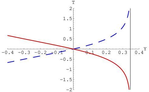
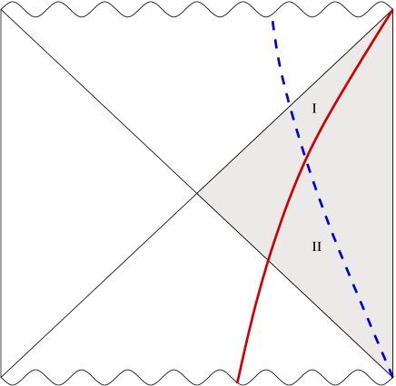
Figure 1: Background brane trajectories for $L=C=1$,$Y_{0}=0$. The trajectory of the positive- (negative-) tension brane is the solid (dashed) line, and the event horizon at $Y=Y_{\mathrm{hor}}$ is denoted by the solid vertical line.

Figure 2: The Penrose diagram corresponding to Fig. 1, i.e. for the case $C>0$. The shaded area denotes the region of extended Schwarzschild-AdS covered by the coordinate system (7). The trajectory of the positive- (negative- ) tension brane is denoted by the solid (dashed) line. The physical region of spacetime is that bounded by the two branes. The diagonal lines bounding the coordinate patch represent the horizon $Y=Y_{\mathrm{hor}}$. Region I therefore represents the portion of the future of the collision which the $Y,T$ coordinates cover.

III.2 Gauge Transformation

We now simplify the analysis of §II to the homogeneous, static background of §III.1. The metric components (7) and the brane trajectories (11) do not, by homogeneity, depend on the spatial coordinates $x^{i}$. We can therefore just leave these coordinates alone, $f^{i}\left(x,y\right)=x^{i}$, and focus on the two-dimensional $Y,T$ portion of the metric. As before, we consider a diffeomorphism

$$T=f\left(y,t\right),\ Y=g\left(y,t\right).$$ (15)

The conditions (4) and (5) on the form of the new metric become

$$g_{y}g_{t} = n(g)^{2}f_{y}f_{t}$$ (16)

$$g_{y}^{2} = n(g)^{2}f_{y}^{2}+d(t)^{2},$$ (17)

giving

$$\mathrm{d}s^{2}=d(t)^{2}\mathrm{d}y^{2}-b\left(y,t\right)^{2}\mathrm{d}t^{2}+a\left(y,t\right)^{2}\mathrm{d}\mathbf{x}^{2}$$ (18)

where

$$b\left(y,t\right)^{2}=n(g)^{2}f_{t}^{2}-g_{t}^{2}.$$

It is at this point that the assumption that the metric (7) is static (i.e. that we are concerned only with Randall-Sundrum-style braneworlds, with no non-gravitational degrees of freedom in the bulk) comes in. This implies that $n$ is only a function of $g$, rather than $n(f,g)$ as would be expected more generally. One can then eliminate $f$ entirely using (16) and (17), giving (up to an arbitrary sign)

$$f_{y} = \frac{1}{n(g)}\sqrt{g_{y}^{2}-d(t)^{2}}$$ (19)

$$f_{t} = \frac{1}{n(g)}\frac{g_{y}g_{t}}{\sqrt{g_{y}^{2}-d(t)^{2}}}$$ (20)

The Jacobian of this coordinate transformation must not vanish, which implies from (19) and (20) that

$$d(t)^{2}g_{t}\neq 0.$$

We can therefore conclude that $g_{t}\neq 0$ away from the collision which, by convention, we shall assume occurs at $T=0$. In the $(y,t)$ plane, the collision corresponds to the vanishing of the metric component $d(t)$, and also to the curve $f(y,t)=0$. This curve has zero proper length, lying at constant $t$, and wlog we can take the collision to correspond to the line $t=0$ on which $f$ vanishes and $g$ takes the constant value $Y_{0}$.
As we saw in §III.1, the distance between the two branes is a monotonically-increasing function after the collision. This implies that one can exploit the $t$-reparameterisation of the metric to fix

$$d(t)=t.$$ (21)

It turns out that this gauge choice ensures the existence of a perturbative expansion of the functions $f$ and $g$ in powers of $t$, as well as corresponding to the linear approximation for close branes used in deRham:2005xv .
Continuity implies that $f_{yt}=f_{ty}$, which from (19) and (20) reduces to a second-order partial differential equation for $g\left(y,t\right)$:

$$g_{t}g_{yy}+t-\frac{g_{y}^{2}}{t}+\frac{n^{\prime}(g)}{n(g)}\left(g_{t}g_{y}^{2}-t^{2}g_{t}\right)=0$$ (22)

Writing (11) as

$$\frac{\mathrm{d}Y_{\pm}}{\mathrm{d}T}=\mp v\left(Y_{\pm}(T)\right),$$

we find

$$\left.g_{t}\right|_{y=0} = \frac{\partial}{\partial t}Y_{+}\left(f(0,t\right)=-\left.v(g)f_{t}\right|_{y=0}$$ (23)

$$\left.g_{t}\right|_{y=1} = \frac{\partial}{\partial t}Y_{-}\left(f(1,t\right)=+\left.v(g)f_{t}\right|_{y=1}$$ (24)

Substituting (20) for $f_{t}$ we find, for example,

$$\left.g_{t}\right|_{y=0} = -\left.\frac{v(g)}{n(g)}\frac{g_{y}\,g_{t}}{\sqrt{g_{y}^{2}-t^{2}}}\right|_{y=0}$$

$$\Rightarrow\left.g_{y}^{2}\right|_{y=0} = \left.\frac{n(g)^{2}t^{2}}{n(g)^{2}-v(g)^{2}}\right|_{y=0}$$

Using (9) and (11) then gives the boundary conditions

$$\left.g_{y}\right|_{y=0,1}=t\left.\frac{a(g)}{n(g)}\right|_{y=0,1}$$ (25)

together with

$$g\left(y,t=0\right)=Y_{0}.$$

Note that the sign of $g_{y}$ in (25) is specified by the choice $f_{t}>0$, $g_{y}>0$, i.e. that the orientation of the new coordinate system is the same as the old one. The fact that the branes are moving in opposite directions, not immediately apparent from the boundary conditions since the $-$ sign in (23) has been lost, follows from the choice of gauge (21).

IV Perturbative expansion in $t$

We now proceed to solve (22) subject to the boundary conditions (25) as a perturbative expansion in powers of $t$. Specifically, we write

$$g\left(y,t\right)=Y_{0}+\sum_{n=1}^{\infty}g_{n}(y)t^{n}$$ (26)

where the boundary conditions (25) will specify the derivatives of $g_{n}$ at $y=0,1$ in terms of the values there of the lower-order $g_{i}$ $(i<n)$. (22) becomes a set of ordinary differential equations for the $g_{n}$; the aim therefore is to identify the correct initial value $g_{n}(0)$ for which the two boundary conditions are simultaneously satisfied. Once $g(y,t)$ has been determined to the required order, $f(y,t)$ can in principle be recovered from (20) with boundary condition $f(y,0)=0$.

IV.1 First order

The $O(t)$ contribution to (22) gives

$$g_{1}g^{\prime\prime}_{1}-{g^{\prime}_{1}}^{2}+1=0$$ (27)

with (25) implying

$$g^{\prime}_{1}(0)=g^{\prime}_{1}(1)=\frac{a_{0}}{n_{0}}$$ (28)

where $a_{0}=a(Y_{0})$ etc. We then obtain the result

$$g_{1}(y)=\frac{1}{2\alpha}\sinh\left(\alpha\left(2y-1\right)\right),\quad\cosh\alpha=\frac{a_{0}}{n_{0}}$$ (29)

The corresponding result for $f$ is

$$f_{1}(y)=\frac{1}{2\alpha n_{0}}\cosh\left(\alpha\left(2y-1\right)\right).$$ (30)

This is just the relevant coordinate transformation in the approximation of constant brane velocities, as detailed in deRham:2005xv .

IV.2 Second order

Before examining the existence of $g_{n}$ for arbitrary $n$, we consider the simpler case of $n=2$.

$$g_{1}g^{\prime\prime}_{2}-2g^{\prime}_{1}g^{\prime}_{2}+2g_{2}g^{\prime\prime}_{1}+\frac{n^{\prime}(Y_{0})}{n(Y_{0})}\left(g_{1}g^{\prime 2}_{1}-g_{1}\right)=0$$ (31)

Expanding out

$$K\left(g(y,t)\right)=K(Y_{0})+t\,g_{1}(y)K^{\prime}(Y_{0})+O(t^{2})$$ (32)

for an arbitrary analytic function $K$, we identify the boundary conditions as

$$g^{\prime}_{2}(y=0,1)=\left.\left(\frac{a}{n}\right)^{\prime}\right|_{Y=Y_{0}}g_{1}(y=0,1)$$

giving

$$g^{\prime}_{2}(1)=-g^{\prime}_{2}(0)=\frac{C\sinh\alpha}{L\alpha n_{0}^{2}a_{0}^{2}}.$$ (33)

There is no simple analytic general solution to this equation, so one must proceed numerically. The task is to find the value of $g_{2}(0)$ such that, after integrating (31) subject to the initial conditions at $y=0$, $g^{\prime}_{2}(1)$ is given by (33), for example using a bisection procedure. The existence of $g_{2}$ is discussed below.

IV.3 General $n$

For tuned tensions, i.e. the boundary conditions (25), the $g_{n}$ all have definite parity $(-1)^{n}$ about $y=1/2$. To show this, we substitute the power series (26) into (22) and consider the coefficient of $t^{n}$, giving

$$g_{1}g^{\prime\prime}_{n}-2g^{\prime}_{1}g^{\prime}_{n}+ng^{\prime\prime}_{1}g_{n}=P_{n}(y)$$ (34)

where $P_{n}(y)$ is composed of a finite sum of products of the $g_{i}$ and their first or second derivatives, but only containing $g_{i}$ for $i<n$ (c.f. (31)). Examining the contributions from the various terms in (22) individually, we write symbolically (i.e. ignoring numerical constants)

$$g_{t}g_{yy}\sim\sum_{k=0}^{\infty}t^{k}\left(\sum_{m=1}^{k}g^{\prime\prime}_{m}\,g_{k+1-m}\right)\supset\sum_{m=2}^{n-1}g^{\prime\prime}_{m}\,g_{n+1-m}$$

where the symbol $\supset$ denotes the terms in the coefficient of $t^{n}$ which do not contain $g_{n}$, i.e. the contribution to the RHS of (34). Working under the inductive hypothesis that $g_{m}$ has parity $(-1)^{m}$ for $m<n$ (which is obviously true for $n=0$ and $n=1$), we see that each summand has the parity $(-1)^{n+1}$. Similarly, $-\frac{1}{t^{2}}g_{y}^{2}$ makes a contribution

$$\frac{1}{t}g_{y}^{2}\supset\sum_{m=2}^{n-1}g^{\prime}_{m}\,g^{\prime}_{n+1-m}$$

Again, the parity of these terms is $(-1)^{n+1}$ by the inductive hypothesis. Next, we examine $g_{t}g_{y}^{2}-t^{2}g_{t}$, which is multiplied by a function of $g$ in (22), so we will need all orders up to $n$ in its expansion. We find that

$$g_{t}g_{y}^{2} \sim \sum_{k=2}^{\infty}t^{k}\left(\sum_{m=1}^{k-1}\sum_{p=1}^{k-m}g_{m}\,g^{\prime}_{p}\,g^{\prime}_{k+1-m-p}\right)$$

$$\sim \sum_{k=2}^{n}t^{k}H_{k}(y)+O(t^{n+1})$$

where $H_{k}(y)$ is a function of parity $(-1)^{k+1}$ involving only $g_{m}$ for $m<k$; there is no contribution at order $t^{n}$ or below from $g_{n}$. $t^{2}g_{t}$ is obviously also of this form, so we just need to look at the $n^{\prime}(g)/n(g)$ term. Any function $K(g)$ with a power series expansion can be written symbolically in the form

$$K(g)\sim K(Y_{0})+\sum_{k=1}^{\infty}t^{k}\left(\sum_{m=1}^{k}\ \sum_{i_{j}>0,\sum i_{j}=k}g_{i_{1}}...g_{i_{k}}\right),$$ (35)

which can be re-expressed as

$$K(g)\sim\left(\sum_{k=0}^{n}t^{k}G_{k}(y)\right)+g_{n}(y)t^{n}+O(t^{n+1})$$

where $G_{k}(y)$ is a sum of products of $g_{i}$ with $i<k$, with total parity $(-1)^{k}$. Putting this all together, we see that the RHS of (34) can be written as

$$P_{n} \sim \sum_{m=2}^{n-1}g^{\prime\prime}_{m}\,g_{n+1-m}+\sum_{m=2}^{n-1}g^{\prime}_{m}\,g^{\prime}_{n+1-m}$$ (36)

$$+\sum_{m=0}^{n-2}G_{m}(y)H_{n-m}(y).$$

Each summand in each term has the same parity, $(-1)^{n+1}$. Therefore, looking back to (34), we see that the whole equation is invariant under parity if $g_{n}$ has parity $(-1)^{n}$. Whether or not this is the case depends on the boundary conditions; in the fine-tuned case, the boundary conditions are just that

$$g^{\prime}_{n}(y_{*})=F_{n-1}(y_{*})$$

where $y_{*}=0,1$ and

$$\frac{a\left(g(y,t)\right)}{n\left(g(y,t)\right)}=\sum_{m=0}^{\infty}F_{n}(y)t^{n}$$

Note that this equation implies that $g^{\prime}_{n}$ at the boundaries is specified entirely in terms of the values there of the $g_{m}$ for $m<n$. From (35), $F_{n-1}(y)$ has parity $(-1)^{n-1}$. Hence

$$g^{\prime}_{n}(1)=(-1)^{n-1}g^{\prime}_{n}(0)$$ (37)

and the inductive hypothesis is proven. One can now show the existence of $g_{n}$ for $n$ odd - since the function will be odd, it and its second derivative must vanish at $y=1/2$. The equation of motion will then prescribe the value of $g^{\prime}_{n}(1/2)$ which, together with $g_{n}(1/2)=0$, will give a unique solution.

For even $n$, one must use a more general argument. We are searching for the value of $g_{n}(0)$ which gives a particular value for $g^{\prime}_{n}(1)$. Taking $g_{n}(0)=N$ for $N$ very large, but $g^{\prime}_{n}(0)$ to its finite, prescribed value, the LHS of (34) will dominate over the RHS apart from at the finite number of points where either $g_{n}$ or its derivatives vanish. Therefore,

$$g_{n}(y)\rightarrow Nh_{n}(y)\ \mathrm{as}\ N=g_{n}(0)\rightarrow+\infty$$ (38)

where $h_{n}$ is the solution to the initial value problem

$$g_{1}f^{\prime\prime}_{n}-2g^{\prime}_{1}f^{\prime}_{n}+ng^{\prime\prime}_{1}f_{n}=0,\quad f_{n}(0)=1,\ f^{\prime}_{n}(0)=0$$

Provided that $h^{\prime}_{n}(1)\neq 0$ (which can be shown numerically for specific values of $n$), we then have that $g^{\prime}_{n}(1)\rightarrow\pm\infty$ as $g_{n}(0)\rightarrow+\infty$, $g^{\prime}_{n}(1)\rightarrow\mp\infty$ as $g_{n}(0)\rightarrow-\infty$. Hence, by continuity, there will be (at least one) intermediate value of $g_{n}(0)$ where $g^{\prime}_{n}(1)$ takes the required value. Hence we can always find a $g_{n}$ satisfying both (34) and the two boundary conditions for $g^{\prime}_{n}$ at $y=0,1$ following from (25).

The above argument is not sensitive to the precise nature of the boundary conditions; in other words, in the case of general brane tensions and brane matter content, the boundary conditions (25) would be modified, but one would still expect to be able to find suitable functions $g_{n}(y)$ to perform the coordinate transformation to the SFB frame.

However, the entire analysis is dependent on the existence of a static bulk frame such as (7) (though the precise nature of the functions $a$ and $n$ will, again, not affect the argument). It is not clear if this result could be generalised to more complicated braneworlds where the bulk is not empty, such as dilatonic or supergravity-inspired models with bulk scalar fields Shiromizu:2004ig ; Kobayashi:2002pw ; Brax:2000xk ; Brax:2002nt ; Mennim:2000wv .

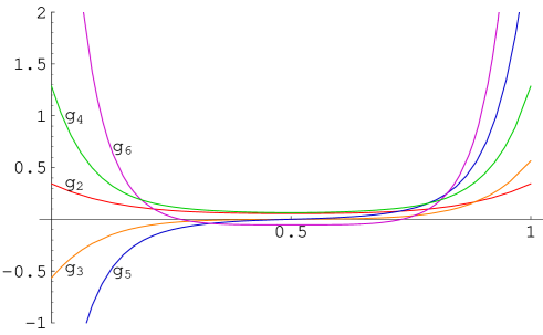
Figure 3: $g_{2}$ to $g_{6}$ plotted for $L=1,C=1,Y_{0}=0$. Note the alternating parities.

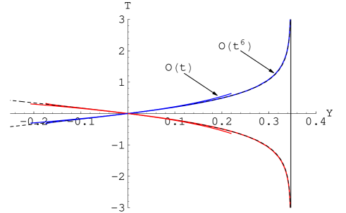
Figure 4: Comparison of the brane trajectories computed using the coordinate transformation function $g(y,t)$ up to $O(t^{6})$ with the exact result. The dotted curves correspond to the exact trajectories as in Fig. 1, showing highly accurate agreement with the numerical results. For comparison the corresponding trajectories computed working only to first order in $t$ are also shown for the same range of $t$, with clear differences.

IV.4 Numerical results and convergence

The horizon structure of the bulk has ramifications for the regions of validity of the coordinate system and the radius of convergence of the power series (26). For $C>0$ there is a horizon, whilst for $C<0$ there is a naked singularity and no consistent embedding of flat, empty, finely-tuned branes. The $C=0$ case, for fine-tuned branes, represents the trivial evolution where the branes remain fixed at their original positions, and the Birkhoff frame automatically satisfies the required gauge conditions (2). We therefore only need consider the case $C>0$.

The first six non-trivial $g_{n}$ have been computed numerically using a bisection procedure to search for $g_{n}(0)$ in the specific case of $Y_{0}=0$, $L=C=1$. The resulting $g_{2}$ to $g_{6}$ are plotted in Fig. 3.

Fig. 4 gives the calculated brane trajectories back in the $(Y,T)$ frame; for example, $g(0,t)$ gives $Y_{-}(t)$, and integrating (20) with $d(t)=t$ gives $f(0,t)=T_{-}(t)$, hence one can plot the trajectories $Y_{\pm}(t)$ and compare them with the exact solutions. The accuracy of the agreement is high, as can be seen from the Fig. 5. Also plotted are the trajectories calculated using only the first-order expression for $g(y,t)$, with the same range of $t$; these clearly differ wildly from the higher-order results as the horizon is approached.

Depending on the initial conditions, either the positive- or negative-tension brane will hit this horizon at a finite value of $t=t_{h}$. For the initial conditions chosen above, this corresponds to $t_{h}\approx 0.36$. At this point, $n(g)$ will vanish at the relevant boundary, and so (22) will break down and one would not expect the coordinate system (18) to be valid beyond this value of $t$. In particular, one would expect this value of $t$ to correspond to the radius of convergence of the series (26). It is clear from Fig. 3 that the boundary values of $g_{n}(y)$ are increasing in modulus as $n$ increases, which is a manifestation of the lack of convergence of the series for large $t$ in this case.

In the fine-tuned, empty-brane case with boundary conditions (25), the symmetry of the problem (i.e. the manifest reflection symmetry under $Y\rightarrow-Y$ in the trajectory plots) implies that the same coordinate system will also be valid before the collision, for $-t_{h}>t>0$.

The advantage of an expansion in the SFB time $t$ is that it is ideally adapted to working in the limit of close branes, a regime of considerable interest recently in the literature McFadden:2005mq ; deRham:2005qg ; deRham:2005xv ; Shiromizu:2002ve ; Battye:2003ks ; Leeper:2005pg . In effect, an expansion in $t$ is equivalent to an expansion in the distance between the two branes. Working even just to first order in $t$ or $d$ whilst making no other approximations, one can obtain interesting, non-perturbative results unattainable using the moduli space approximation deRham:2005qg ; deRham:2005xv . Whether or not the full series (26) converges is then not important if one simply wants to proceed perturbatively in $t$.

V Perturbative expansion in C

An alternative method of finding the required gauge (2) is to consider an expansion in the velocity of the branes (11). Specifically, we define the parameter

$$h=\sqrt{C}$$ (39)

and expand in this rather than in $t$. This amounts to an expansion about the $C=0$ AdS spacetime where the (finely-tuned) branes are at fixed positions in the Birkhoff frame (7). This method turns out to be conceptually and analytically simpler than the expansion in $t$, though it is of less direct use for the near-brane regime, being an expansion about a static configuration. In this sense, working to linear order in $h$ will reproduce the results of the moduli space approximation.

As discussed below, we will in fact expand about the state where the branes are static and coincident, in order to simplify the analysis somewhat and to tie in with the rest of the paper assuming that the branes are moving apart from an initial collision. It would not, however, be difficult to generalise the results to a different initial configuration.

V.1 Formalism

Firstly we define a new coordinate $Z=e^{-Y/L}$, in terms of which the Birkhoff frame metric can be written

$$\mathrm{d}s^{2} = \frac{L^{2}}{Z^{2}}\mathrm{d}Z^{2}-n(Z)^{2}\mathrm{d}T^{2}+a(Z)^{2}\mathrm{d}\mathbf{x}^{2}$$ (40)

$$a(Z)^{2} = Z^{2}+\frac{h^{2}}{4Z^{2}}$$

$$n(Z)^{2} = a(Z)^{2}-\frac{h^{2}}{a(Z)^{2}}$$ (41)

For $h=0$ the branes are static, at $Z=Z^{(+)}_{0}$ and $Z=Z^{(-)}_{0}$. Since we are interested in modelling the aftermath of a collision we shall take $Z^{(\pm)}_{0}=Z_{0}$. Whilst simplifying the resulting analysis considerably one must then remember that, for $h=0$, the metric will be singular. Therefore we shall expect $g_{yy}$ in the SFB frame (18) to vanish for $h=0$. Bearing this in mind, we then perform a coordinate transformation as before, keeping the $t$-gauge general for the time being (as opposed to the choice $d(t)=t$ of the previous section). Expanding in $h$, we write

$$Z(y,t) = Z_{0}\left(1+\sum_{n=1}^{\infty}h^{n}Z_{n}(y,t)\right)$$ (42)

$$T(y,t) = t+\sum_{n=1}^{\infty}h^{n}T_{n}(y,t),$$ (43)

where for $h=0$ we can set $T=t$ since the branes are already at fixed positions. We then solve

$$\partial_{y}g_{yy}=g_{yt}=0$$

order by order to determine the functions $Z_{n}(y,t)$ and $T_{n}(y,t)$, together with the boundary conditions (11),

$$\frac{\mathrm{d}Z_{\pm}}{\mathrm{d}T}=\pm Z_{\pm}\frac{h}{L}\frac{n(Z_{\pm})}{a(Z_{\pm})^{2}}$$ (44)

V.2 First order

In the $(y,t)$ frame, the metric becomes

$$\mathrm{d}s^{2} = \left(\frac{L^{2}}{Z^{2}}Z_{y}^{2}-n(Z)^{2}T_{y}^{2}\right)\mathrm{d}y^{2}$$

$$+2\left(\frac{L^{2}}{Z^{2}}Z_{y}Z_{t}-n(Z)^{2}T_{y}T_{t}\right)\mathrm{d}y\mathrm{d}t$$

$$+\left(\frac{L^{2}}{Z^{2}}Z_{t}^{2}-n(Z)^{2}T_{t}^{2}\right)\mathrm{d}t^{2}+a(Z)^{2}\mathrm{d}\mathbf{x}^{2}$$

and so, using (42) and (43), we obtain

$$\partial_{y}g_{yy} = 2\left(L^{2}\dot{Z}_{1}Z^{\prime\prime}_{1}-Z_{0}^{2}\,\dot{T}_{1}T^{\prime\prime}_{1}\right)h^{2}+O\left(h^{3}\right)$$ (46)

$$g_{yt} = -Z_{0}^{2}\dot{T}_{1}h+O(h^{2}).$$ (47)

Next we examine the boundary conditions (44),

$$\frac{\mathrm{d}Z_{+}}{\mathrm{d}T} = \frac{\partial_{t}Z(0,t)}{\partial_{t}T(0,t)}=Z_{0}\dot{Z}_{1}(0,t)h+O(h^{2})$$

$$= Z_{+}\frac{h}{L}\frac{n(Z_{+})}{a(Z_{+})^{2}}=\frac{h}{L}+O(h^{2})$$

giving

$$\vspace{-3mm}\dot{Z}_{1}(0,t)=\frac{1}{LZ_{0}}$$ (48)

and, similarly,

$$\dot{Z}_{1}(1,t)=-\frac{1}{LZ_{0}}.$$ (49)

(47) gives the simple condition that $\dot{T_{1}}=0$ and, choosing the collision to occur at $t=0$, implies

$$T_{1}(y,t)=0.$$ (50)

The condition (46) on $g_{yy}$ reduces to

$$Z^{\prime\prime}_{1}=0$$

which, together with the boundary conditions (48), (49) and $Z_{1}(y,0)=Z_{0}$, gives

$$Z_{1}(y,t)=\frac{t}{LZ_{0}}\left(1-2y\right)$$ (51)

Therefore, to $O(h)$, the required coordinate transformation is

$$Z(y,t) = Z_{0}+\frac{ht}{L}\left(1-2y\right)+O(h^{2})$$ (52)

$$T(y,t) = t+O(h^{2}).$$

The metric (V.2) is then given by

$$\mathrm{d}s^{2} = \left(4\frac{t^{2}h^{2}}{Z_{0}^{2}}+O(h^{3})\right)\mathrm{d}y^{2}+O(h^{2})\,\mathrm{d}y\mathrm{d}t$$

$$+\left(Z_{0}^{2}+2\frac{Z_{0}t}{L}\left(1-2y\right)h+O(h^{2})\right)\left(-\mathrm{d}t^{2}+\mathrm{d}\mathbf{x}^{2}\right)$$

which, to $O(h)$, is of the required form (2). As a check, we can calculate the proper times on the two branes,

$$\mathrm{d}t_{\pm}=\left(Z_{0}\pm\frac{ht}{L}+O(h^{2})\right)\mathrm{d}t$$ (54)

giving the Hubble parameters as

$$H_{\pm}=\pm\frac{h}{LZ_{0}^{2}}+O(h^{2}).$$ (55)

The function $d(t)$, giving the proper distance between the branes along lines of constant $y$, can be read off from (V.2) as

$$d(t)=\frac{2t}{Z_{0}}h+O(h^{2})$$ (56)

which gives

$$H_{\pm}=\pm\frac{1}{2L}\frac{\mathrm{d}}{\mathrm{d}t_{\pm}}d(t)+O(h^{2}),$$ (57)

in agreement with the low-energy result of deRham:2005xv .

V.3 Higher orders

The analysis at higher orders is straightforward. The constraint $\partial_{y}g_{yy}=0$ reduces to an equation of the form

$$Z^{\prime\prime}_{n}(y,t)=\sum_{i,j}^{\mathrm{fin}}c^{(n)}_{ij}t^{i}y^{j}$$ (58)

where the superscript means that the sum is finite, i.e. a binomial in $y$ and $t$. This can easily be integrated to obtain $Z_{n}(y,t)$ up to two arbitrary functions of $t$, which are fixed by the boundary conditions (44) and the requirement that $Z(y,0)=Z_{0}$. Similarly, the other constraint $g_{yt}=0$ is of the form

$$T^{\prime}_{n}(y,t)=\sum_{i,j}^{\mathrm{fin}}d^{(n)}_{ij}t^{i}y^{j}$$ (59)

giving $T_{n}(y,t)$ up to an arbitrary function of $t$. This is a manifestation of the $t$-reparameterisation invariance, and can be fixed for example by setting $T(t,0)=t$. In this particular gauge, the next two sets of functions are

$$Z_{2}(y,t) = \frac{2t^{2}}{L^{2}Z_{0}^{2}}y(y-1)$$ (60)

$$T_{2}(y,t) = -\frac{2t}{Z_{0}^{4}}y(1-y)$$ (61)

$$Z_{3}(y,t) = \frac{t}{L^{3}Z_{0}^{5}}\left\{4\left(L^{2}+t^{2}Z_{0}^{2}\right)\left(\frac{y^{2}}{2}-\frac{y^{3}}{3}\right)\right.$$

$$\qquad\quad\left.+y\left(\frac{7}{12}L^{2}-\frac{2}{3}t^{2}Z_{0}^{2}\right)-\frac{5}{8}L^{2}\right\}$$

$$T_{3}(y,t) = \frac{2t^{2}y}{3LZ_{0}^{5}}\left(9-12y+8y^{2}\right).$$ (63)

This transformation satisfies all the required boundary conditions, as well as the conditions on the metric (2), up to $O(h^{3})$:

$$g_{yy} =4\frac{t^{2}h^{2}}{Z_{0}^{2}}+\frac{h^{4}t^{2}}{3L^{2}Z_{0}^{6}}\left(8\,t^{2}\,Z_{0}^{2}-19L^{2}\right)+O(h^{5})$$

$$g_{yt} =O(h^{4})$$

In order to prove the relations (58) and (59), we use induction. Specifically, we aim to prove that the general form of $Z_{n}$ and $T_{n}$ is a binomial function of $t$ and $y$ of the form

$$Z_{n}(y,t) =t\sum_{i,j=0}^{\mathrm{fin}}a^{(n)}_{ij}y^{i}t^{j}\quad\mathrm{for\ }n\geq 1$$ (64)

$$T_{n}(y,t) =y\,t\sum_{i,j=0}^{\mathrm{fin}}b^{(n)}_{ij}y^{i}t^{j}\quad\mathrm{for\ }n\geq 2.$$ (65)

From (51) and (60-63), we see that this is indeed the case for $n\leq 3$. We now assume that we have found the $Z_{m}$ and $T_{m}$ for $m<n$, satisfying the required boundary conditions. We then look at the constraint that $g_{yy}$ is independent of $y$, which becomes

$$ZZ_{y}Z_{yy}=Z_{y}^{3}+\frac{1}{L^{2}}\left(n(Z)n^{\prime}(Z)Z^{3}Z_{y}T_{y}^{2}+n(Z)Z^{3}T_{y}T_{yy}\right).$$ (66)

We aim for an equation of the form (58) and, examining the LHS of this equation, we see that the lowest order in $h$ at which $Z^{\prime\prime}_{n}$ appears is at $O(h^{n+1})$,

$$ZZ_{y}Z_{yy} \supset \left(Z_{0}^{3}\,Z_{1}^{\prime}Z_{n}^{\prime\prime}+t^{2}B(y,t)\right)h^{n+1}$$ (67)

$$= \left(-\frac{2t}{L}Z_{0}^{2}Z_{n}^{\prime\prime}+t^{2}B(y,t)\right)h^{n+1}$$

where the symbolic notation $B(y,t)$ represents a binomial function in $t$ and $y$ depending only on the binomial functions $Z_{m}$ for $m<n$. The factor of $t^{2}$ multiplying this function is displayed explicitly since we need to keep track of powers of $t$ to ensure the RHS of (58) is indeed a binomial with no negative powers of $t$. Now starting on the RHS of (66), we note that

$$Z_{y}^{3}=Z_{0}^{3}\sum_{a,b,c=1}^{\infty}h^{a+b+c}Z^{\prime}_{a}\,Z^{\prime}_{b}\,Z^{\prime}_{c}$$

and hence, at $O(h^{n+1})$, does not contain $Z^{\prime}_{n}$, only the lower $Z_{m}$. Hence we can write symbolically

$$Z_{y}^{3}=t^{3}B(y,t).$$

Both $T_{y}^{2}$ and $T_{y}T_{yy}$ have a factor $t^{2}\,h^{4}$ in front, and can be written with the inductive hypothesis as

$$T_{y}^{2},\ T_{y}T_{yy}\ \sim\ t^{2}h^{4}B(y,t)+t^{2}O(h^{n+2}).$$ (68)

Furthermore, as in (35), a general analytic function of $Z$ can be written

$$f(Z)=f(Z_{0})+\sum_{k=1}^{\infty}h^{k}\left(\sum_{m=1}^{k}\sum_{i_{j}>0,\sum{i_{j}}=k}Z_{i_{1}}...Z_{i_{k}}\right)$$ (69)

Combining (68) and (69), we see that the term with coefficient $1/L^{2}$ on the RHS of (66) contributes, at $O(h^{n+1})$, a term of the form $t^{2}B(y,t)$.

Hence, putting all of the above together, we have shown that $Z_{n}$ is given in terms of the $Z_{m}$ for $m<n$ by an equation of the form (58) with an additional pre-factor of $t$. This equation can always be integrated to give

$$Z_{n}(y,t)=tB_{n}(y,t)+a_{n}(t)y+b_{n}(t)$$ (70)

where $B_{n}(y,t)$ is a binomial expression depending on the $Z_{m}$ for $m<n$, and $a_{n}(t)$ and $b_{n}(t)$ are arbitrary functions, which are then uniquely fixed by the boundary conditions. Unlike the expansion in $t$, we can in principle calculate all the $Z_{n}$ analytically, though this is not a terribly helpful procedure. What is important is that the boundary conditions are trivial to implement - (44) will prescribe values for $Z^{\prime}_{n}$ at $y=0$ and $y=1$, which, together with $Z(y,0)=Z_{0}$, fix $a_{n}(t)$ and $b_{n}(t)$ uniquely from (70).

To show the existence of the $T_{n}$, we need to examine the equation

$$T_{y}\,T_{t}=\frac{L^{2}}{Z^{2}n(Z)^{2}}Z_{y}Z_{t}$$ (71)

which follows from the metric (V.2). $T_{n}$ enters the LHS at $O(h^{n})$,

$$T_{y}\,T_{t}\supset h^{n}\left(T^{\prime}_{n}+B(y,t)\right)$$

where again $B(y,t)$ stands for binomial terms composed of already-known functions, the $T_{m}$ for $m<n$ in this case. In fact the RHS of (71) does not contain $Z_{n}$ at $O(h^{n})$, since both $Z_{y}$ and $Z_{t}$ are $O(h)$. Therefore, the equation for $T_{n}$ is of the form (59), specifically

$$T^{\prime}_{n}(y,t)=t\,C_{n}(y,t)$$

with the factor of $t$ coming from the $Z_{y}$. This can be integrated to

$$T_{n}(y,t)=y\,t\,\tilde{C}_{n}(y,t)+d_{n}(t)$$ (72)

where once again $\tilde{C}_{n}$ is a binomial function of $y$ and $t$. The arbitrary function $d_{n}(t)$ encodes the $t$ reparameterisation invariance of the gauge. Because of the pre-factor $y$ in (72), the gauge $T(0,t)=t$ corresponds to setting $d_{n}(t)=0$. We have therefore shown that there exist simple, binomial expressions for $T_{n}(y,t)$ and $Z_{n}(y,t)$ for all $n$, with an extremely simple if tedious procedure for finding them explicitly.

It should be emphasised, as in §IV, that the precise nature of the boundary conditions are not important. Hence, although the explicit solution constructed in this section corresponds to empty, fine-tuned branes, it would be simple in principle to repeat the process for more general situations with both de-tuned branes and matter at the background level.

VI Cosmological Perturbations

We now consider more general spacetimes, where the spatial homogeneity is broken by cosmological perturbations. Our starting point is to consider a general background spacetime, taking the metric to be of the form

$$\mathrm{d}s_{0}^{2}=\mathrm{d}Y^{2}-n(Y,T)^{2}\mathrm{d}T^{2}+a(Y,T)^{2}\Omega_{ij}\mathrm{d}x^{i}\mathrm{d}x^{j}$$ (73)

where $\Omega_{ij}$ is the relevant maximally-symmetric spatial metric of constant curvature. In this frame the branes are taken to have loci $Y_{\pm}(T)$. We then assume that a coordinate transformation

$$T=f(y,t),\quad Y=g(y,t)$$ (74)

can be constructed as described previously, satisfying

$$g_{y}g_{t}-n(f,g)^{2}f_{y}f_{t}=0,$$ (75)

$$g_{y}^{2}-n(f,g)^{2}f_{y}^{2}=d(t)^{2},$$ (76)

with boundary conditions

$$g\left(y=0,t\right)=Y_{-}\left(f(y=0,t)\right),$$

$$g\left(y=1,t\right)=Y_{+}\left(f(y=1,t)\right),$$

bringing the metric into the standard form

$$\mathrm{d}s_{0}^{2}=d(t)^{2}\mathrm{d}y^{2}-b(y,t)^{2}\mathrm{d}t^{2}+a(y,t)^{2}\Omega_{ij}\mathrm{d}x^{i}\mathrm{d}x^{j}$$ (77)

with the branes fixed at $y=0$ and $y=1$ (the precise forms of $b(y,t)$ and $a(y,t)$ are not important). Note that, in this section, we shall not fix the $t$-reparameterisation invariance as in (21), which will allow us to consider more general situations than the branes moving apart after a collision, such as perturbations about static branes.

We now allow the presence of cosmological perturbations, both to the background metric (73) and, in the case of scalar perturbations, to the positions of the branes themselves. We then attempt to find an infinitesimal gauge transformation which will not only retain the properties

$$g_{5\mu}=\frac{\partial}{\partial y}g_{55}=0$$ (78)

of the metric, but bring the brane positions back to $y=0$ and $y=1$ if necessary. Firstly, we shall perform the coordinate transformation (74) to bring the background into the form (77), before constructing the gauge transformation required to accommodate both the brane positions and the bulk metric perturbations into the SFB gauge at first order. Note that, in this section, we are still not considering any non-gravitational degrees of the freedom in the bulk, which would in principle also need perturbing, such as a bulk scalar field.

VI.1 Tensor perturbations

Firstly, we consider the simplest case of tensor perturbations. In five dimensions, the most general infinitesimal tensor perturbation vandeBruck:2000ju to (73) only affects the transverse spatial components, i.e.

$$g_{ij}\rightarrow a(Y,T)^{2}\left(\Omega_{ij}+h_{ij}\right)\mathrm{d}x^{i}\mathrm{d}x^{j}.$$ (79)

This will therefore not affect the properties (78) of the metric in the new frame (77). Furthermore, the brane trajectories are scalars, and are therefore not affected by a purely tensor perturbation. Hence tensor perturbations can trivially be accommodated into the gauge (77).

VI.2 Vector perturbations

There are six vector degrees of freedom for five-dimensional perturbations about the background (73), encoded in three divergenceless vectors:

$$\mathrm{d}s^{2} = \mathrm{d}s_{0}^{2}+Q^{(T)}_{i}\mathrm{d}x^{i}\mathrm{d}T+Q^{(Y)}_{i}\mathrm{d}x^{i}\mathrm{d}Y$$

$$+a(Y,T)^{2}F_{(i|j)}\mathrm{d}x^{i}\mathrm{d}x^{j}$$

where $|$ denotes the covariant derivative with respect to the metric $\Omega_{ij}$ and $F^{i}_{|i}=Q^{(Y)i}_{|i}=Q^{(T)i}_{|i}=0$. Performing the background coordinate transformation (74), we obtain the perturbed version of (77)

$$\mathrm{d}s^{2} = d(t)^{2}\mathrm{d}y^{2}-b(y,t)^{2}\mathrm{d}t^{2}+\left(Q^{(T)}_{i}f_{y}+Q^{(Y)}_{i}g_{y}\right)\mathrm{d}y\mathrm{d}x^{i}$$

$$+\left(Q^{(T)}_{i}f_{t}+Q^{(Y)}_{i}g_{t}\right)\mathrm{d}t\mathrm{d}x^{i}$$

$$+a(y,t)^{2}\left(\Omega_{ij}+2F_{(i|j)}\right)\mathrm{d}x^{i}\mathrm{d}x^{j}$$

Therefore, in order to satisfy the gauge conditions (78), we require the linear combination

$$Q^{(T)}_{i}f_{y}+Q^{(Y)}_{i}g_{y}$$ (81)

to vanish. Under the most general infinitesimal vector gauge transformation

$$x^{i}\rightarrow x^{i}+\eta^{i},\quad\eta^{i}_{|i}=0,$$

the three vector perturbations transform as

$$\delta Q^{(Y)}_{i} = -a(y,t)^{2}\partial_{y}\eta_{i}$$

$$\delta Q^{(T)}_{i} = -a(y,t)^{2}\partial_{t}\eta_{i}$$

$$\delta F_{i} = -\eta_{i}$$

where $\eta_{i}=\Omega_{ij}\eta^{j}$. There are therefore two gauge-invariant vector perturbations (i.e. four degrees of freedom) corresponding to $Q^{(Y)}_{i}-a^{2}F^{\prime}_{i}$ and $Q^{(T)}_{i}-a^{2}\dot{F}_{i}$, and any one vector perturbation can be set to zero. In particular, we can remove the linear combination (81) with suitable $\eta_{i}$ satisfying

$$f_{y}\partial_{y}\eta_{i}+g_{y}\partial_{t}\eta_{i}=\frac{1}{a(y,t)^{2}}\left(Q^{(T)}_{i}f_{y}+Q^{(Y)}_{i}g_{y}\right).$$

Again there is no vector perturbation to the brane trajectories, hence these still lie at $y=0$ and $y=1$.

VI.3 Scalar perturbations

Scalar perturbations require a more detailed treatment, both because there are more of them in general and because one must also assume that the brane positions are perturbed. In five dimensions there are seven scalar degrees of freedom,

$$\mathrm{d}s^{2} = \mathrm{d}s_{0}^{2}+\phi_{55}\mathrm{d}Y^{2}+2\phi_{05}\mathrm{d}Y\mathrm{d}T-n^{2}(Y,T)\phi_{00}\mathrm{d}T^{2}$$ (82)

$$+Q^{(Y)}_{,i}\mathrm{d}Y\mathrm{d}x^{i}+Q^{(T)}_{,i}\mathrm{d}T\mathrm{d}x^{i}$$

$$+2\,a(y,t)^{2}\left(2\,\psi+E_{,ij}\right)\mathrm{d}x^{i}\mathrm{d}x^{j}$$

Three of these can be removed at this stage by a scalar gauge transformation; effectively, this is just the statement that one can always choose a Gaussian-Normal gauge for the bulk where the off-diagonal terms $Q^{(Y)}_{,i}$, $\phi_{05}$ and the $g_{55}$ perturbation vanish:

$$\mathrm{d}s_{GN}^{2} = \mathrm{d}s_{0}^{2}-n^{2}(Y,T)\phi\,\mathrm{d}T^{2}+Q^{(T)}_{,i}\mathrm{d}T\mathrm{d}x^{i}$$ (83)

$$+2\,a(y,t)^{2}\left(2\,\psi+E_{,ij}\right)\mathrm{d}x^{i}\mathrm{d}x^{j}$$

where $\phi\equiv\phi_{00}$. Performing the coordinate transformation (74), we find

$$\mathrm{d}s^{2} = \left[d(t)^{2}-n^{2}f_{y}^{2}\phi\right]\mathrm{d}y^{2}-2n^{2}f_{y}f_{t}\phi\,\mathrm{d}y\mathrm{d}t+Q_{,i}f_{y}\mathrm{d}x^{i}\mathrm{d}y$$ (84)

$$-\left(b^{2}+n^{2}f_{t}^{2}\phi\right)\mathrm{d}t^{2}+Q_{,i}f_{t}\mathrm{d}x^{i}\mathrm{d}t$$

$$+a^{2}\left[(1+\psi)\Omega_{ij}+E_{,ij}\right]\mathrm{d}x^{i}\mathrm{d}x^{j}$$

where all the problematic terms have been written out in the first line, and $n=n(y,t)\equiv n\left(f(y,t),g(y,t)\right)$ etc. The background brane positions are fixed in this frame, but in the presence of scalar perturbations will be displaced to

$$y_{+}\left(\mathbf{x},t\right)=\delta y_{+}\left(\mathbf{x},t\right),\quad y_{-}\left(\mathbf{x},t\right)=1+\delta y_{-}\left(\mathbf{x},t\right)$$ (85)

In five dimensions there are four gauge-invariant scalar degrees of freedom, hence we cannot eliminate any more of these perturbation variables with gauge transformations. We can, however, perform another gauge transformation to rearrange them in such a way as to satisfy the conditions (78), whilst simultaneously bringing the two branes back to the fixed positions $y=0$ and $y=1$. Under the most general infinitesimal scalar coordinate transformation

$$x^{a}\rightarrow x^{a}+\xi^{a},\quad\xi^{a}=\left(\xi,\chi,\partial^{i}\zeta\right),$$ (86)

the metric perturbations transform as

$$\delta g_{55} = -2d^{2}\xi^{\prime}-2d\dot{d}\,\chi$$

$$\delta g_{50} = -d^{2}\dot{\xi}+b^{2}\chi^{\prime}$$

$$\delta g_{5i} = -\partial_{i}\left[\zeta^{\prime}+d^{2}\xi-2\frac{a^{\prime}}{a}\zeta\right]$$

where ${}^{\prime}=\partial_{y}$ and $\dot{}=\partial_{t}$. Hence, from (84), we find the three conditions necessary to fix the required gauge:

$$2d^{2}\xi^{\prime\prime}+2d\dot{d}\,\chi^{\prime}+\left(n^{2}\,f_{y}^{2}\,\phi\right)^{\prime}=0,$$ (87)

$$\zeta^{\prime}+d^{2}\xi-2\frac{a^{\prime}}{a}\zeta-Qf_{y}=0$$ (88)

$$b^{2}\chi^{\prime}-d^{2}\dot{\xi}-n^{2}\,f_{y}\,f_{t}\,\phi=0,$$ (89)

together with the boundary conditions

$$\xi\left(y=0\right)=-\delta y_{+}\left(\mathbf{x},t\right),\quad\xi\left(y=1\right)=-\delta y_{-}\left(\mathbf{x},t\right)$$ (90)

which, from (85), will bring the brane positions to $y=0$ and $y=1$. $\zeta$ and $\chi$ have no boundary conditions to satisfy; once one has found the required $\xi$, they follow immediately from (88) and (89) respectively. Eliminating $\chi^{\prime}$ from (87) with (87), we obtain the equation of motion for $\xi$,

$$\xi^{\prime\prime}+k(y,t)\dot{\xi} =F(y,t,\mathbf{x})$$ (91)

$$F(y,t,\mathbf{x}) \equiv\frac{\left(n^{2}\,f_{y}^{2}\,\phi\right)^{\prime}}{2d^{2}}-\frac{n^{2}d\dot{d}}{b^{2}\,t}\,f_{y}f_{t}\,\phi$$

$$k(y,t) \equiv\frac{d\dot{d}}{b^{2}}$$

Interestingly only one of the original seven possible five-dimensional perturbations appears in this equation. In principle some information about the values of $\phi$ and its derivatives at the boundaries can be inferred from the Israël junction conditions, though in practice this is not relevant. The perturbation is absorbed into a ‘forcing’ term $F(y,t,\mathbf{x})$, with (91) taking the form of a generalised diffusion equation.

VI.3.1 Perturbations about static branes

For static Randall-Sundrum branes (e.g. $C=0$ for empty branes), the original background configuration (73) is already in an SFB gauge with $d(t)=1$. In this simple case, the equation of motion (91) reduces to

$$\xi^{\prime\prime}=F(y,t,\mathbf{x})$$ (92)

The general solution of this equation is

$$\xi(y,t,\mathbf{x})=\xi^{\mathrm{P}}(y,t,\mathbf{x})+(1-y)A(\mathbf{x},t)+y\,B(\mathbf{x},t),$$ (93)

where $\xi^{\mathrm{P}}$ is a particular solution to (92), and the linear term represents the most general homogeneous solution. $A(\mathbf{x},t)$ and $B(\mathbf{x},t)$ are arbitrary functions which can be set so that $\xi$ satisfies arbitrary boundary conditions at $y=0$ and $y=1$. In particular, one can always solve the boundary conditions (90) with the choice

$$A(\mathbf{x},t) = -\left(\delta y_{+}(\mathbf{x},t)+\xi^{\mathrm{P}}(0,t,\mathbf{x})\right)$$ (94)

$$B(\mathbf{x},t) = -\left(\delta y_{-}(\mathbf{x},t)+\xi^{\mathrm{P}}(1,t,\mathbf{x})\right)$$

Hence any cosmological perturbations about a static, fixed-brane background can always be accommodated into an SFB gauge.

VI.3.2 Perturbations about general backgrounds

For non-trivial $k(y,t)$ the process of constructing a solution to (91) for arbitrary boundary conditions (90) is far more complicated and one must, once again, resort to a series solution. The boundary conditions (90) can be dealt with by a simple redefinition of the forcing function $F(y,t,\mathbf{x})$, by setting

$$\xi(y,t,\mathbf{x})=w(y,t,\mathbf{x})-(1-y)\delta_{+}(\mathbf{x},t)-y\,\delta_{-}(\mathbf{x},t).$$ (95)

The new function $w$ has the simpler boundary conditions that $w=0$ at $y=0$ and $y=1$, and satisfies the equation

$$w^{\prime\prime}+k(y,t)\dot{w}=G(y,t,\mathbf{x})$$ (96)

where

$$G(y,t,\mathbf{x})\equiv F(y,t,\mathbf{x})+k(y,t)\left((1-y)\delta y_{+}(\mathbf{x},t)+y\,\delta y_{-}(\mathbf{x},t)\right)$$

We now expand the functions $G$, $w$ and $k$ in powers of $t$. Considering the case once again where the branes are moving apart after a collision which occurred at $t=0$, we see from its definition in (91) that $k(y,0)=0$, hence there is no $t^{0}$ term in its expansion. We therefore write

$$k(y,t) = \sum_{t=1}^{\infty}t^{n}k_{n}(y)$$

$$G(y,t,\mathbf{x}) = \sum_{t=0}^{\infty}t^{n}G_{n}(y,\mathbf{x})$$

$$w(y,t,\mathbf{x}) = \sum_{t=0}^{\infty}t^{n}w_{n}(y,\mathbf{x}),$$

which, upon substitution into (96), gives

$$w^{\prime\prime}_{0} = G_{0}$$ (97)

$$w^{\prime\prime}_{n}+nk_{1}w_{n} = G_{n}-\sum_{m=1}^{n-1}m\,w_{m}\,k_{n+1-m}\equiv\tilde{G}_{n}$$ (98)

together with the boundary conditions

$$w_{n}(0,\mathbf{x})=w_{n}(1,\mathbf{x})=0.$$

(98) is just a simple, linear Sturm-Liouville problem which can always be solved with an eigenfunction expansion subject to certain conditions. Specifically, we consider the eigenfunction equation

$$\phi_{m}^{\prime\prime}(y)+\lambda_{m}k_{1}(y)\phi_{m}(y)=0,\quad\phi_{m}(0)=\phi_{m}(1)=0.$$ (99)

The eigenfunctions $\phi_{m}$ for $m=1,2,3...$ will form a complete, orthogonal basis, and so we can expand

$$\tilde{G}_{n}(y,t,\mathbf{x}) = k_{1}(y)\sum_{m}G_{nm}(\mathbf{x},t)\,\phi_{m}(y),$$

$$\quad w_{n}(y,t,\mathbf{x}) = \sum_{m}w_{nm}(\mathbf{x},t)\,\phi_{m}(y)$$

and these sums converge absolutely. Substituting these expressions back into (98), we find

$$w_{nm}=\frac{G_{nm}}{n-\lambda_{m}}$$ (100)

and hence the required solution to (91) subject to the boundary conditions (90) has been constructed. From (100), we see that this solution only exists if the eigenvalues of (99) are either never integer-valued, or, if $\lambda_{m}=N$ for some integer $N$, then the corresponding $G_{Nm}$ vanishes.

Note that this conclusion is consistent with $t$-reparameterisation. For example, if we reparameterise

$$t\rightarrow T(t)=T_{1}\,t+T_{2}\,t^{2}+...$$

then

$$k_{1}(y)\rightarrow\frac{k_{1}(y)}{N}$$

where $N$ is the minimal positive integer such that $T_{N}\neq 0$. The eigenvalues of (99) will therefore all be multiplied by $N$, and $G_{nm}$ is only non-zero for $n$ a multiple of $N$. Hence the conclusion remains the same. This condition on the functions $k(y,t)$ and $G(y,t,\mathbf{x})$ can be regarded as necessary and sufficient for scalar perturbations to be accommodated within the SFB gauge.

Note that if $k_{1}(y)=0$, the above argument will simplify considerably since each equation for $w_{n}$ will just be of the form

$$w^{\prime\prime}_{n}=\tilde{G}_{n}\qquad\mathrm{for\ }k_{1}=0$$

which can be integrated immediately, with two arbitrary constants to fix the boundary conditions. Hence, in this case, it will always be possible to find the required gauge. However, for branes moving apart after a collision, from the above argument $k_{1}(y)$ will be proportional always to its value $1/b(y,0)$ in the gauge $d(t)=t$, which will not vanish. Hence one will have to check the eigenspectrum of the problem to verify the existence of the required SFB gauge.

The precise nature of the function $G(y,t,x)$ encoding both the bulk perturbation $\phi$ and the perturbations $\delta y_{\pm}$ to the brane positions is not important for the above discussion. Hence one would expect, subject to the above caveats, to be able to include the effects of matter perturbations on the brane if desired. Since the perturbative construction of the background coordinate transformation in §§IV and V were not sensitive to the precise nature of the boundary conditions either, one can expect to include matter at the background level as well. Hence we have presented in this paper a method for constructing SFB gauges very generally for Randall-Sundrum cosmologies.

VII Conclusions

The aim of this paper was to demonstrate the existence of gauges for Randall-Sundrum two-brane braneworlds in which the metric takes the particularly simple form (2) whilst, at the same time, the branes are located at fixed positions. Such gauges have been assumed to exist already in the literature Kanno:2002ia2 ; deRham:2005qg ; deRham:2005xv ; Shiromizu:2002ve , without proof, since they simplify considerably the analysis of the five-dimensional Einstein equations necessary to derive analytic results for effective theories.

We first examined the dynamics of the system in the background, deriving from the trajectories of the branes the necessary boundary conditions for the coordinate transformation functions. These were then found using two different power series expansions, expanding either in time or in the parameter $\sqrt{C}$ related to the mass of the bulk black hole.

The former approach corresponds to an expansion in the radion, the proper distance between the two branes, and is adapted ideally to the case of two branes moving apart soon after a collision. This regime is of interest in recent attempts to model the Big Bang as a collision between two branes Khoury:2001wf ; Khoury:2001bz ; Gibbons:2005rt ; Jones:2002cv ; Turok:2004gb ; Tolley:2003nx ; Steinhardt:2002ih ; Kanno:2002py . However, the non-linear equations which one needs to solve order by order in $t$ do not admit an analytic solution. One can, however, demonstrate the existence of all terms in the series, satisfying the required boundary conditions, corresponding to being able to perform the necessary coordinate transformation correct to $O(t^{N})$ for arbitrary $N$. Whilst no analytic information about the convergence of the series is possible, numerical simulations show good agreement with the exact results, and we conjectured that the radius of convergence of the series would be equal to $t_{h}$, the time taken for the first brane to hit the horizon.

A second method, namely an expansion in $\sqrt{C}$, corresponds to an expansion in the velocity of the branes. It is possible to obtain analytic expressions for the coordinate transformation functions, and the resulting SFB metric, correct to arbitrary order in $h$. This is because the equations at each order are simple, linear differential equations, involving just binomial functions which are trivial to integrate.

Results on cosmological backgrounds are of limited interest; the important question is whether or not one can find an infinitesimal gauge transformation to accommodate arbitrary cosmological perturbations, at first order, into an SFB gauge. We addressed this question last, and showed that this is trivially the case for tensor and vector perturbations. Scalar perturbations require considerably more work because one must also take into account a perturbation of the brane trajectories themselves, and hence impose boundary conditions on the infinitesimal coordinate transformation $\xi=\delta x^{5}$. The second-order partial differential equation for $\xi$ can be solved by an eigenvalue expansion, giving a well-defined constraint on the eigenvalues of (99) for the SFB gauge to exist.

Whilst the arguments in this paper do not apply to braneworlds with a ‘non-empty’ bulk (i.e. with non-gravitational bulk degrees of freedom), they are not sensitive to the precise nature of the Israel junction conditions; one can include both detuned tensions and brane matter without altering the conclusions.

Acknowledgements:

The author would like to thank Anne Davis for her supervision and Claudia de Rham for her considerable help in the preparation of this manuscript. He is supported by Trinity College, Cambridge.

References

- (1) P. Brax, C. van de Bruck and A. C. Davis, Rept. Prog. Phys. 67 (2004) 2183 [arXiv:hep-th/0404011].
- (2) D. Langlois, Prog. Theor. Phys. Suppl. 148 (2003) 181 [arXiv:hep-th/0209261].
- (3) P. Binetruy, C. Deffayet and D. Langlois, Nucl. Phys. B 565 (2000) 269 [arXiv:hep-th/9905012].
- (4) P. Binetruy, C. Deffayet and D. Langlois, Nucl. Phys. B 615, 219 (2001) [arXiv:hep-th/0101234].
- (5) Y. b. Kim, C. O. Lee, I. b. Lee and J. J. Lee, arXiv:hep-th/0307023.
- (6) R. Maartens, Living Rev. Rel. 7 (2004) 7 [arXiv:gr-qc/0312059].
- (7) L. Randall and R. Sundrum, Phys. Rev. Lett. 83 (1999) 3370 [arXiv:hep-ph/9905221].
- (8) A. Lukas, B. A. Ovrut, K. S. Stelle and D. Waldram, Nucl. Phys. B 552, 246 (1999) [arXiv:hep-th/9806051].
- (9) A. Lukas, B. A. Ovrut and D. Waldram, Phys. Rev. D 60, 086001 (1999) [arXiv:hep-th/9806022].
- (10) A. Lukas, B. A. Ovrut and D. Waldram, Phys. Rev. D 61, 023506 (2000) [arXiv:hep-th/9902071].
- (11) T. Shiromizu, Y. Himemoto and K. Takahashi, Phys. Rev. D 70 (2004) 107303 [arXiv:hep-th/0405071].
- (12) S. Kobayashi and K. Koyama, JHEP 0212, 056 (2002) [arXiv:hep-th/0210029].
- (13) P. Brax and A. C. Davis, Phys. Lett. B 497, 289 (2001) [arXiv:hep-th/0011045].
- (14) P. Brax, C. van de Bruck, A. C. Davis and C. S. Rhodes, Phys. Rev. D 67 (2003) 023512 [arXiv:hep-th/0209158].
- (15) P. Horava and E. Witten, Nucl. Phys. B 475 (1996) 94 [arXiv:hep-th/9603142].
- (16) C. van de Bruck, M. Dorca, R. H. Brandenberger and A. Lukas, Phys. Rev. D 62 (2000) 123515 [arXiv:hep-th/0005032].
- (17) R. Maartens, arXiv:astro-ph/0402485.
- (18) L. E. Mendes and A. Mazumdar, Phys. Lett. B 501 (2001) 249 [arXiv:gr-qc/0009017].
- (19) J. Khoury and R. J. Zhang, Phys. Rev. Lett. 89 (2002) 061302 [arXiv:hep-th/0203274].
- (20) T. Shiromizu and K. Koyama, Phys. Rev. D 67 (2003) 084022 [arXiv:hep-th/0210066].
- (21) S. Kanno and J. Soda, Phys. Rev. D 66, 043526 (2002) [arXiv:hep-th/0205188].
- (22) S. Kanno and J. Soda, Phys. Rev. D 66 (2002) 083506 [arXiv:hep-th/0207029].
- (23) S. L. Webster and A. C. Davis, arXiv:hep-th/0410042.
- (24) G. A. Palma and A. C. Davis, Phys. Rev. D 70 (2004) 106003 [arXiv:hep-th/0407036].
- (25) G. A. Palma and A. C. Davis, Phys. Rev. D 70 (2004) 064021 [arXiv:hep-th/0406091].
- (26) C. de Rham, Phys. Rev. D 71 (2005) 024015 [arXiv:hep-th/0411021].
- (27) G. Calcagni, JCAP 0311, 009 (2003) [arXiv:hep-ph/0310304].
- (28) P. L. McFadden, N. Turok and P. J. Steinhardt, arXiv:hep-th/0512123.
- (29) R. Maartens, D. Wands, B. A. Bassett and I. Heard, Phys. Rev. D 62 (2000) 041301 [arXiv:hep-ph/9912464].
- (30) D. Langlois, R. Maartens and D. Wands, Phys. Lett. B 489 (2000) 259 [arXiv:hep-th/0006007].
- (31) A. R. Liddle and A. N. Taylor, Phys. Rev. D 65 (2002) 041301 [arXiv:astro-ph/0109412].
- (32) K. Koyama, D. Langlois, R. Maartens and D. Wands, JCAP 0411 (2004) 002 [arXiv:hep-th/0408222].
- (33) C. de Rham and S. Webster, Phys. Rev. D 72 (2005) 064013 [arXiv:hep-th/0506152].
- (34) C. de Rham and S. Webster, Phys. Rev. D 71 (2005) 124025 [arXiv:hep-th/0504128].
- (35) T. Shiromizu, K. Koyama and K. Takahashi, Phys. Rev. D 67, 104011 (2003) [arXiv:hep-th/0212331].
- (36) J. Khoury, B. A. Ovrut, P. J. Steinhardt and N. Turok, Phys. Rev. D 64 (2001) 123522 [arXiv:hep-th/0103239].
- (37) J. Khoury, B. A. Ovrut, N. Seiberg, P. J. Steinhardt and N. Turok, Phys. Rev. D 65 (2002) 086007 [arXiv:hep-th/0108187].
- (38) G. W. Gibbons, H. Lu and C. N. Pope, [arXiv:hep-th/0501117].
- (39) N. Jones, H. Stoica and S. H. H. Tye, JHEP 0207 (2002) 051 [arXiv:hep-th/0203163].
- (40) N. Turok, M. Perry and P. J. Steinhardt, Phys. Rev. D 70 (2004) 106004 [Erratum-ibid. D 71 (2005) 029901] [arXiv:hep-th/0408083].
- (41) A. J. Tolley, N. Turok and P. J. Steinhardt, Phys. Rev. D 69 (2004) 106005 [arXiv:hep-th/0306109].
- (42) P. J. Steinhardt and N. Turok, Science 296 (2002) 1436.
- (43) S. Kanno, M. Sasaki and J. Soda, Prog. Theor. Phys. 109, 357 (2003) [arXiv:hep-th/0210250].
- (44) M. Bucher and C. Carvalho, Phys. Rev. D 71 (2005) 083511 [arXiv:hep-th/0412064].
- (45) P. Binetruy, C. Deffayet, U. Ellwanger and D. Langlois, Phys. Lett. B 477 (2000) 285 [arXiv:hep-th/9910219].
- (46) G. Niz and N. Turok, arXiv:hep-th/0601007.
- (47) A. Mennim and R. A. Battye, Class. Quant. Grav. 18 (2001) 2171 [arXiv:hep-th/0008192].
- (48) R. A. Battye, C. Van de Bruck and A. Mennim, Phys. Rev. D 69 (2004) 064040 [arXiv:hep-th/0308134].
- (49) E. Leeper, K. Koyama and R. Maartens, Phys. Rev. D 73 (2006) 043506 [arXiv:hep-th/0508145].