hep-th/0603253

Bicocca-FT-06-5

Deformations of Toric Singularities and Fractional Branes

Agostino Butti

Dipartimento di Fisica, Università di Milano-Bicocca
P.zza della Scienza, 3; I-20126 Milano, Italy

Fractional branes added to a large stack of D3-branes at the singularity of a Calabi-Yau cone modify the quiver gauge theory breaking conformal invariance and leading to different kinds of IR behaviors. For toric singularities admitting complex deformations we propose a simple method that allows to compute the anomaly free rank distributions in the gauge theory corresponding to the fractional deformation branes. This algorithm fits Altmann’s rule of decomposition of the toric diagram into a Minkowski sum of polytopes. More generally we suggest how different IR behaviors triggered by fractional branes can be classified by looking at suitable weights associated with the external legs of the (p,q) web. We check the proposal on many examples and match in some interesting cases the moduli space of the gauge theory with the deformed geometry.

 agostino.butti@mib.infn.it

1 Introduction and overview

The study of the IR gauge theory on a stack of regular D3 or fractional branes placed at a Calabi-Yau singularity is an important issue to test the AdS/CFT correspondence and its extensions to non conformal cases.

Many concrete examples has recently been found: the superconformal gauge theory dual to type IIB string theory on $AdS_{5}\times Y^{p,q}$ was built in [1]; see [2, 3, 4] for $AdS_{5}\times L^{p,q,r}$. The Sasaki-Einstein metrics for $Y^{p,q}$ and $L^{p,q,r}$ can be found in [5] and [6, 7] respectively. At the same time many general features of the correspondence were uncovered, especially for toric Calabi-Yau singularities: the new techniques of dimers, perfect matchings, zig-zag paths [8, 9] allow to represent a complicated superconformal quiver gauge theory with simple diagrams and to compute from them the dual geometry, represented by a toric diagram, or vice-versa. Therefore it was also possible to perform detailed and general checks of the correspondence [10, 11, 12, 13, 14, 15, 16, 17, 18, 19]. Alternative techniques for the study of Calabi-Yau singularities are based on exceptional collections [20, 21].

A well known method to break conformal invariance is to add fractional branes, that can be seen as higher dimensional branes wrapping collapsed cycles at the singularity. On the gauge theory side the fractional branes modify the number of colors of different gauge groups consistently with cancellation of anomalies for gauge symmetries. In many known examples [22, 23, 24] fractional branes lead to cascades of Seiberg dualities that reduce the number $N$ of regular branes, so that the IR dynamics is dominated by fractional branes.

A classification of fractional branes into three different classes according to the IR behavior they produce in the gauge theory was proposed in [25]. We may have i) fractional deformation branes, that describe a complex deformation of the dual geometry and produce a supersymmetric (typically confining) vacuum in field theory; ii) $\mathcal{N}=2$ fractional branes, leading to $\mathcal{N}=2$ dynamics in some regions of the moduli space of the gauge theory and iii) supersymmetry breaking (SB) fractional branes, that seem to be the most common kind of fractional branes: a supersymmetric vacuum is no more present and typically one finds a runaway behavior [25, 26, 27, 28, 29].

In general there is a great number of fractional branes that can be consistently added to a quiver gauge theory: in the toric case there are $d-3$ fractional branes, where $d$ is the perimeter of the toric diagram of the dual geometry. Therefore one would need a simple method to compute the anomaly free rank distributions corresponding to the three classes of fractional branes. In this paper we propose an algorithm to do that in the general toric case. We will use the language of dimers and zig-zag paths.

First of all we use the known correspondence between fractional branes, that is anomaly free rank distributions in the gauge theory, and the $d-3$ baryonic symmetries of the original superconformal theory (without fractional branes) [30]. Then the main idea of this paper is to parametrize the global symmetries, and among them the baryonic symmetries, using weights $b_{i}$ assigned to the external legs $v_{i}$ of the (p,q) web, or equivalently to the zig-zag paths in the dimer configuration. The global charge of any link in the dimer is computed by the difference of the two weights of the zig-zag paths to which the link belongs.

It is then easy to understand to which class of fractional branes a rank distribution in the gauge theory belongs by looking at the weights of the corresponding baryonic symmetry. We will treat in great detail the case of deformation branes: even though the deformation of a toric Calabi-Yau cone is no more a toric manifold, having only $U(1)^{2}$ isometries, there is a simple rule based only on toric data to understand whether a toric cone admits a complex structure deformation. In fact deformations of isolated Gorenstein singularities are in correspondence with Minkowski decompositions of the toric diagram [31] or equivalently with splittings of the (p,q) web into sub-webs in equilibrium. Our proposal is that fractional branes corresponding to such deformed geometries have constant weights $b_{i}$ on the different sub-webs.

$\mathcal{N}=2$ fractional branes instead are possible when there is a not isolated singularity, that is when in the (p,q) web there are parallel vectors perpendicular to the same edge of the toric diagram. In our proposal the baryonic symmetries associated with $\mathcal{N}=2$ fractional branes have non-zero weights only on these parallel vectors.

We also suggest that different assignments of weights $b_{i}$ correspond to SB fractional branes.

We check these proposals on concrete examples. In particular for theories admitting complex deformations, when a single deformation parameter is turned on, we show that gauge groups have the only possible ranks: $SU(N)$, $SU(N+M)$, $SU(N-M)$ (previously in the literature only cases with $SU(N)$ and $SU(N+M)$ gauge groups were known); moreover in these cases our proposal for deformation branes leads to configurations where no gauge group can develop an ADS superpotential term, and therefore the existence of a supersymmetric vacuum is expected. In this analysis we also use the splitting into sub-webs at the level of zig-zag paths in the dimer, that has already been observed in a recent paper [32].

If we add fractional deformation branes we should not only check that our proposal leads to a supersymmetric vacuum, but also that the quantum modified moduli space of the gauge theory, when probed by a regular brane, is equal to the complex deformation of the toric singularity. For some examples of such computations in the literature see [22, 24]; interesting are the techniques used in [33], since they should work for all toric cases admitting deformations. One has to write the moduli space of vacua through F-term relations in the chiral ring of mesonic operators, that are typically modified at quantum level by ADS terms; on the geometric side the linear relations in $C^{*}$ (the dual of the toric fan $C$) expressing the toric manifold as a (non complete) intersection in a complex space can be modified using Altmann’s results [31].

We study the example of the $PdP_{4}$ theory, admitting two complex deformation parameters, in order to verify that our proposal for computing the rank distribution for fractional deformation branes reproduces correctly also the deformed geometry. In performing these computations we make use of the $\Psi$-map, recently introduced in [21], since it allows to find the precise mapping between mesons in the chiral ring and integer points in $C^{*}$, as already noted in the same paper.

Therefore we translate the $\Psi$-map theory in [21] in the language of charges and zig-zag paths. We also note that the idea of giving weights to zig-zag paths allows to prove explicitly that the $\Psi$-map of a closed loop is an affine function and that the flavor charges of mesons are proportional to the homotopy numbers of the corresponding loops in the torus, as observed for the first time in [12].

This paper is organized as follows. Section 2 contains the definitions of useful tools like dimers, zig-zag paths and the algorithms for distributing charges in the dimer [15, 34]. In Section 3 we review the classification of fractional branes according to the IR behavior [25] and the Minkowski decomposition of toric diagrams. In Section 4 we explain in great detail the correspondence between anomaly free rank distributions in the dimer and baryonic symmetries of the superconformal theory [30]; we also prove that the correspondence is one to one. In Section 5 we introduce the parametrization of global charges through weights for zig-zag paths and we characterize the three classes of fractional branes through the weights of the associated baryonic symmetries. We check this proposal for computing rank distributions in many examples in Section 6, where we also treat the general case of theories with a single deformation parameter turned on. Section 7 contains useful comments to the $\Psi$-map theory [21]. In Section 8 we provide the explicit computation for $PdP_{4}$ of the moduli space of the gauge theory with fractional branes that matches the deformed geometry.

2 Generalities about the gauge theory

In this Section we briefly review some results about the AdS/CFT correspondence in the superconformal case that have been recently obtained for toric geometries. To be concrete we will explain the ideas on a specific example well known in the literature: the Suspended Pinch Point (SPP) that we will use also in the following Sections.

We consider $N$ D3-branes living at the tip of a CY cone. The base of the cone, or horizon, is a five-dimensional compact Sasaki-Einstein manifold $H$ [35, 36]. The IR limit of the gauge theory living on the branes is ${\cal N}=1$ superconformal and dual in the AdS/CFT correspondence to the type IIB background $AdS_{5}\times H$, which is the near horizon geometry.

The problem of finding the low energy gauge theory dual to a generic Calabi-Yau singularity is difficult and still unsolved, but recently the AdS/CFT correspondence has been built for a wide class of CY singularities: the toric CY cones (roughly speaking a six dimensional manifold is toric if it has at least $U(1)^{3}$ isometries).

Many geometrical informations about toric CY cones are encoded in the toric diagram, a convex polygon in the plane with integer vertices. For the SPP example the fan $C$ is generated by the integer vectors $V_{i}$:

$$(0,0,1)\quad(1,0,1)\quad(1,1,1)\quad(0,2,1)$$ (2.1)

and the corresponding toric diagram is drawn in Figure 1. The (p,q) web is the set of vectors perpendicular to the edges of the toric diagram and with the same length as the corresponding edges (see Figure 2).

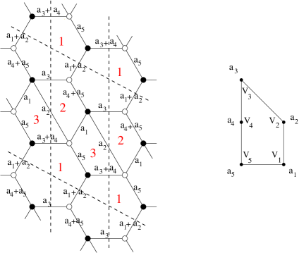
Figure 1: Dimer configuration and toric diagram for the Suspended Pinch Point.

In the toric case the gauge theory is completely identified by the periodic quiver, a diagram drawn on $T^{2}$ (it is the “lift” of the usual quiver to the torus): nodes represent $SU(N)$ gauge groups, oriented links represent chiral bifundamental multiplets and faces represent the superpotential: the trace of the product of chiral fields of a face gives a superpotential term (with a sign + or - if the arrows of the face in the periodic quiver are oriented clockwise or anticlockwise respectively).

Equivalently the gauge theory is described by the dimer configuration, or brane tiling, the dual graph of the periodic quiver, drawn also on a torus $T^{2}$. In the dimer the role of faces and vertices is exchanged: faces are gauge groups and vertices are superpotential terms. The dimer is a bipartite graph: it has an equal number of white and black vertices (superpotential terms with sign + or - respectively) and links connect only vertices of different colors.

The dimer for SPP is drawn in Figure 1: it has three faces $F=3$, seven edges $E=7$, and four vertices $V=4$. The three gauge groups are labelled by the red numbers in Figure 1: faces with the same number are identified. The fundamental cell of the torus $T^{2}$ where the dimer lies is (any of) the parallelogram formed by the dashed lines. Since the dimer is on a torus we have: $V-E+F=0$.

By applying Seiberg dualities to a quiver gauge theory we can obtain different quivers that flow in the IR to the same CFT: to a toric diagram we can associate different quivers/dimers describing the same physics. It turns out that one can always find phases where all the gauge groups have the same number of colors; these are called toric phases. Seiberg dualities keep constant the number of gauge groups $F$, but may change the number of fields $E$, and therefore the number of superpotential terms $V=E-F$. We will call minimal toric phases those having the minimal number of fields $E$.

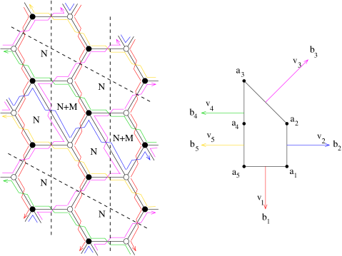
Figure 2: Zig-zag paths for the Suspended Pinch Point and their correspondence with external legs of the (p,q) web.

If the dimer is known the toric diagram can be reconstructed using perfect matchings. A perfect matching is a subset of links in the dimer such that every white and black vertex is taken exactly once. Perfect matchings can be mapped to integer points of the toric diagram through the Kasteleyn matrix which counts their (oriented) intersections with two loops generating the fundamental group of the torus [8].

The inverse problem of reconstructing the dimer from the toric diagram can be solved using zig-zag paths [9] (see also [39]). A zig-zag path in the dimer is a path of links that turn maximally left at a node, maximally right at the next node, then again maximally left and so on [9]. We draw them in the specific case of SPP theory in Figure 2: they are the five loops in red, blue, magenta, green and yellow and they are drawn so that they intersect in the middle of a link as in [39]. Note that every link of the dimer belongs to exactly two different zig-zag paths, oriented in opposite directions. Moreover for dimers representing consistent theories the zig-zag paths are closed non-intersecting loops. There is a one to one correspondence between zig-zag paths and legs of the $(p,q)$ web: the homotopy class in the fundamental group of the torus of every zig-zag path is given by the integer numbers $(p,q)$ of the corresponding leg in the $(p,q)$ web [9]. The reader can check this in the example of Figure 2. Note that there are two distinct zig-zag paths with homotopy numbers (-1,0) and not a unique path with homotopy (-2,0) that would intersect itself. This is a general feature of theories with a toric diagram having integer points on its edges.

The Fast Inverse Algorithm of [9] consists just in drawing the zig-zag paths on a fundamental cell with the appropriate homotopy numbers and satisfying suitable consistency conditions.

2.1 Distribution of charges in the dimer

Non anomalous $U(1)$ symmetries play a very important role in the gauge theory. Here we review how to count and parametrize them and how to compute the charge of a certain link in the dimer.

For smooth horizons $H$ we expect $d-1$ global non anomalous symmetries, where $d$ is the number of sides of the toric diagram in the dual theory. We can count these symmetries from the number of massless vectors in the $AdS$ dual. Since the manifold is toric, the metric has three $U(1)$ isometries. One of these (generated by the Reeb vector) corresponds to the R-symmetry while the other two give two global flavor symmetries in the gauge theory. Other gauge fields in $AdS$ come from the reduction of the RR four form on the non-trivial three-cycles in the horizon manifold $H$, and there are $d-3$ three-cycles in homology [4] when $H$ is smooth. On the field theory side, these gauge fields correspond to baryonic symmetries. Summarizing, the global non anomalous symmetries are:

$$U(1)^{d-1}=U(1)^{2}_{F}\times U(1)^{d-3}_{B}$$ (2.2)

If the horizon H is not smooth (that is the toric diagram has integer points lying on the edges), equation (2.2) is still true with $d$ equal to the perimeter of the toric diagram in the sense of toric geometry (d = number of vertices of toric diagram + number of integer points along edges). For instance in the SPP theory $d=5$, so that there are 2 baryonic symmetries.

These $d-1$ global non anomalous charges can be parametrized by $d$ parameters $a_{1},a_{2},\ldots,a_{d}$ [15], each associated with a vertex of the toric diagram or a point along an edge (see Figure 2 for SPP), satisfying the constraint:

$$\sum_{i=1}^{d}a_{i}=0$$ (2.3)

The $d-3$ baryonic charges are those satisfying the further constraints [4]:

$$\sum_{i=1}^{d}a_{i}V_{i}=0$$ (2.4)

where $V_{i}$ are the vectors of the fan: $V_{i}=(x_{i},y_{i},1)$ with $(x_{i},y_{i})$ the coordinates of integer points along the perimeter of the toric diagram.

As an aside recall that R-symmetries are parametrized with the $a_{i}$ having total sum 2 instead of zero.

There are two simple equivalent algorithms to compute the charge of a generic link in the dimer in function of the parameters $a_{i}$ (the equivalence of the two algorithms was shown in [34], assuming a conjecture in [9]).

The first efficient way to find the distribution of charges [15], valid for all toric phases, is based on perfect matchings: the parameters $a_{i}$ are associated with vertices of the toric diagram, and to every vertex $V_{i}$ there corresponds a single perfect matching in the dimer, at least for physical theories [15, 9]. Therefore the charge of a link in the dimer can be computed as the sum of the parameters $a_{i}$ of all the external perfect matchings (corresponding to vertices) to which the link belongs. For examples of how to use this prescription using the Kasteleyn matrix, see [15].

The second algorithm is based on zig-zag paths [34]. Consider the two zig-zag paths to which a link in the dimer belongs. They correspond to two vectors $v_{i}=(p_{i},q_{i})$ and $v_{j}=(p_{j},q_{j})$ in the $(p,q)$ web. Then the charge of the link is given by the sum of the parameters $a_{i+1}+a_{i+2}\ldots+a_{j}$ between the vectors $v_{i}$ and $v_{j}$ . So for instance in Figure 2 the links corresponding to the intersection of the red and the magenta zig-zag paths (vectors $v_{1}$ and $v_{3}$ in the (p,q) web) have charge equal to $a_{1}+a_{2}$.

This rule explains the formula for the multiplicities of fields with a given charge [15]: since every link in the dimer corresponds to the intersection of two zig-zag paths, the number of fields with charge $a_{i+1}+a_{i+2}\ldots+a_{j}$ is equal to the number of intersections between the zig zag paths corresponding to $v_{i}$ and $v_{j}$, which is just $\mathrm{det}(v_{i},v_{j})$.

3 Classes of fractional branes and deformations
in toric geometry

In this Section we review the classification [25] of the different types of IR behaviors that fractional branes can induce in the gauge theory. We also explain Altmann’s rule for understanding deformations of toric singularities [31] .

Let us start with a large number $N$ of regular $D3$-branes at the singularity of a toric CY cone. The IR limit of the gauge theory on the branes is superconformal and the dual geometry is $AdS_{5}\times H$. A well known method to break the conformal symmetry is to add fractional branes. Fractional branes may be thought as higher dimensional branes wrapping collapsed cycles at the singularity. From the dual string theory point of view they add new fluxes and change the $AdS$ geometry [22, 23]: the only known example of smooth metric describing the near horizon geometry produced by fractional branes is the Klebanov-Strassler solution [22], relative to fractional branes at the tip of the conifold ($H=T^{1,1}$); the internal metric is the CY metric over the deformed conifold up to a warp factor.

It is easier to study fractional branes from the gauge theory point of view: in this case they are described by a modification of the number of colors of the different gauge groups in the quiver gauge theory (with the only requirement that gauge symmetries are still anomaly free). Maybe it is simpler to see this on the mirror description [39]: the mirror of the apex of the cone (where the $T^{3}$ fibration of the toric manifold is completely degenerate) is a “pinched” $T^{3}$ made up of a collections of $F$ intersecting $S^{3}$, where $F$ is the number of gauge groups. D3 regular, and D5, D7 fractional branes at the singularity are mapped in the mirror to D6-branes wrapping the $S^{3}$’s: in particular the $N$ D3 branes are mapped to D6-branes wrapping all the $S^{3}$’s, contributing to the same factor of $N$ to the number of colors of gauge groups, whereas fractional branes wrap only some of the $S^{3}$, modifying the rank distribution.

In this paper when speaking of fractional branes we will always refer to this changing of rank distribution in the quiver gauge theory.

The IR behavior of quiver gauge theories with fractional branes have been studied in many examples, for recent works see [24, 25, 26, 27, 32]. In [25] a general classification of fractional branes was accordingly proposed:

• Deformation fractional branes: They are present when the dual toric geometry admits a complex structure deformation according to Altmann’s rule and they describe the gauge theory dual to the geometry of the deformed cone. In fact when there is no obstruction to a deformation, we may expect the existence of a CY metric over the deformed cone and a supergravity solution similar to the Klebanov-Strassler solution. The gauge theory has therefore a supersymmetric vacuum ($\mathcal{N}=1$). In concrete examples it turns out that these fractional branes lead to a cascading behavior: after a certain number of Seiberg dualities the gauge theory comes back to itself with the number of regular branes decreased by some amount of fractional branes $N\rightarrow N-M$. Typically in the IR one finds a certain number of isolated confining gauge groups with no more bifundamental matter.

• $\mathcal{N}=2$ fractional branes: They are present when there are integer points along the sides of a toric diagram. In this case the horizon $H$ is not smooth and the singularity at the tip of the cone is not isolated. A side of the toric diagram with $k-1$ internal points gives rise to a complex line of $\mathbb{C}^{2}/\mathbb{Z}_{k}$ singularities in the toric cone passing through the origin, along which the fractional branes can move. The dual gauge theory has flat directions where the dynamics has an accidental $\mathcal{N}=2$ supersymmetry. The behavior is really different from the case of deformation branes, for example the SPP theory with an $\mathcal{N}=2$ fractional brane, corresponding to Figure 8 c), does not seem to have a cascade.

• Supersymmetry breaking (SB) fractional branes: They seem to be the most generic anomaly free distributions of ranks for gauge groups; they are present also when the toric cone admits a deformation, in fact the number of complex structure deformations is less (or at most equal, see the KS theory) than the number of possible fractional branes (= number of baryonic symmetries in the original superconformal theory = $d-3$). Their main feature is that the gauge theory does not have a supersymmetric vacuum[25, 26, 27, 28, 29]: typically in the IR, when the number of colors has decreased after the cascade, some gauge group have $N_{f}<N_{c}$ and develops ADS superpotential terms leading to a runaway behavior.

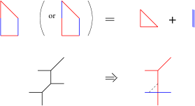
Figure 3: Deformation of the cone over SPP: decomposition of the toric diagram in Minkowski summands and splitting of the web into subwebs in equilibrium.

In Section 5 we will explain how to find the rank distributions corresponding to these kinds of fractional branes.

Let us now briefly explain Altmann’s rule for deformations of toric singularities. In [31] it is shown that the complex deformations of isolated Gorenstein (i.e. CY) toric singularities are completely characterized by the possible decompositions of the toric diagram into a Minkowski sum of polytopes. We will deal the case of 6d toric cones, described by toric diagrams on a 2-plane. Given two 2d convex polygons $P_{1}$, $P_{2}$, one can define their Minkowski sum $P_{1}+P_{2}$ as the convex hull of the set $\{p=p_{1}+p_{2}|\,p_{1}\in P_{1},p_{2}\in P_{2}\}$, that is the set of points obtained by summing the points of the two polygons. One can realize that the edges of $P$ are the union of the sets of edges of the polygons $P_{1}$ and $P_{2}$.

We give an example in Figure 3, where we show the decomposition of the toric diagram of SPP into two Minkowski summands (note however that this singularity is not isolated, and hence one can identify the sides of the triangle in red in two different ways into the original SPP toric diagram, compare with Figures 8 a) and b)).

It is possible to read the same decomposition in terms of subdivision of the (p,q) web into two (or more) sub-webs at equilibrium, that is the perpendiculars to the sides of the toric diagram are divided into subsets where the sum of vectors is still zero. We show this in the same Figure 3: the two legs in blue are lifted from the plane of the other vectors and the link between the two subwebs represents a three-cycle (one deformation parameter). Therefore the cone over SPP has $d-3=2$ fractional branes and a branch of complex deformations with one parameter.

In Figure 4 we report the example of the cone over $dP_{3}$. We see that there are two possible decompositions into Minkowski summands, that is two branches of complex structure deformations: the first one, Figure 4 a), has one parameter (separation into two sub-webs). The second branch, Figure 4 b) has two parameters (separation into three subwebs). The number of fractional branes for this theory is $d-3=3$.

Toric cones whose toric diagram has no Minkowski decompositions do not admit complex structure deformations.

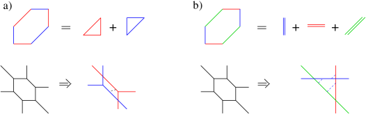
Figure 4: Deformation of the cone over $dP_{3}$. a) One parameter branch. b) Two parameters branch.

4 Fractional branes and baryonic symmetries

In this Section we explain in detail the known correspondence between fractional branes and baryonic symmetries in the gauge theory [30]. We also prove that the correspondence is one to one.

As explained in the previous Section, fractional branes in the quiver gauge theory modify the number of colors of the gauge groups in such a way that the gauge symmetries are still anomaly free; in fact the number of flavors for every gauge group is equal to the number of anti-flavors. These anomaly free configurations can be computed through the (integer) kernel of the antisymmetric intersection matrix $S_{ij}$ defining the quiver:

$$\sum_{j}S_{ij}\,n_{j}=0$$ (4.1)

where in this Section the indexes $i,j$ label the gauge groups, that is the nodes of the periodic quiver. $n_{j}$ is the number of colors of j-th gauge group, and the entry $(i,j)$ of the intersection matrix $S_{ij}$ is the number of arrows going from node $i$ to $j$ minus the number of arrows going from $j$ to $i$. In the following we will assume to start from a toric phase of the original superconformal gauge theory (before introducing fractional branes), that is a phase where all the gauge groups have the same number of colors $SU(N)$. Therefore the constant vector $n_{j}=N$ is always in the kernel of $S$ and it describes regular D3-branes.

There is an equivalent way to compute the allowed distributions of colors $n_{i}$ based on baryonic symmetries. Consider a rank assignment $n_{i}$ as in (4.1). Define for every oriented link $X$ of the periodic quiver a charge $c(X)$:

$$c(X_{i\rightarrow j})=n_{j}-n_{i}$$ (4.2)

if the field $X$ goes from node $i$ to node $j$. Note that adding regular branes does not change the charges of chiral fields.

The charges in (4.2) can be seen as linear combinations of the $U(1)$ parts of the original $U(N)$ gauge groups: the charge associated with the i-th $U(1)$ gauge group is $+1$ ($-1$) for links entering (exiting) in the i-th node and zero for other fields. The sum of these charges with weight $n_{i}$ for each node $i$ gives the distribution in (4.2).

It is easy to see that (4.2) defines a global non anomalous (baryonic) $U(1)$ charge of the original superconformal gauge theory, that is the theory with all groups equal to $SU(N)$. First of all note that from (4.2) it follows that the total charge of every closed loop of links in the periodic quiver is zero (this is true also if the arrows are not all oriented in the same direction: we simply define the charge of a loop by subtracting the charges of links oriented in the opposite direction). In particular faces of the periodic quiver are closed loops and represent superpotential terms, and hence the superpotential is conserved.

To check that the symmetry is non anomalous under every gauge transformation we have to compute for every gauge group $i$ the sum of the charges of all links attached to node $i$; this is given by:

$$\sum_{j}S_{ij}\,c(X_{i\rightarrow j})=\sum_{j}S_{ij}\,n_{j}-\sum_{j}S_{ij}\,n_{i}=0$$ (4.3)

which vanishes because of (4.1) and because the original phase is toric.

Vice versa every global non anomalous $U(1)$ symmetry (with integer coefficients) such that every closed loop (oriented or not) has charge zero defines a rank assignment satisfying (4.1): start from a generic gauge group $i$ and fix its rank to an arbitrary integer $n_{i}$. Then the rank of a node $j$ connected to $i$ by a path $L$ is obtained as:

$$n_{j}=n_{i}+c(L_{i\rightarrow j})$$ (4.4)

Since the charge of closed loops is zero, this rank assignment is unambiguous. Moreover from the fact that the $U(1)$ symmetry is non anomalous in the original superconformal theory, that is $\sum_{j}S_{ij}\,c(X_{i\rightarrow j})=0$, we find that equation (4.1) is satisfied (look at the first equality in (4.3)). Note that all ranks are defined up to a common constant, that can be varied by adding regular branes. Equation (4.4) or (4.2) also shows that global $U(1)$ symmetries that assign zero charge to all closed (oriented or not) loops are automatically linear combinations of the $U(1)$ parts of the original $U(N)$ gauge groups.

Therefore we have a one to one correspondence between fractional branes (4.1) and non anomalous global $U(1)$ symmetries that assign zero charge to all closed loops. It is known in the literature that such symmetries are the baryonic symmetries (of the theory with all $SU(N)$ gauge groups). As an evidence for this recall that mesonic operators in the superconformal field theory are dual to supergravity states in string theory, whereas baryonic operators, having a conformal dimension proportional to $N$, correspond to states of a D3-brane wrapped over opportune three cycles of the horizon manifold $H$. Therefore only baryons can be charged under a baryonic symmetry, that in the string theory dual comes from the reduction of RR four form along three cycles in $H$. Instead mesonic operators, that are closed oriented loops, have zero charge under baryonic symmetries.

In Section 7, we will give a direct proof in the gauge theory for the toric case that the $d-3$ baryonic symmetries are exactly the symmetries under which all loops (also non oriented) have zero charge. Instead the charges of loops under the two flavor symmetries are proportional to the homotopy numbers of the loops in the torus $T^{2}$ where the periodic quiver is drawn.

5 Matching deformations with fractional branes

In this Section we propose a simple method to find the rank distribution of gauge groups in the gauge theory dual to the geometry produced by fractional deformation branes, when the toric singularity admits a complex-structure deformation according to Altmann’s rule. We will also extend the proposal to $\mathcal{N}=2$ branes.

First of all we have to find the baryonic symmetry associated with the fractional brane and then reconstruct the ranks of the gauge groups as explained in the previous Section, equation (4.4).

The main idea is to change the parametrization of global charges: instead of using the parameters $a_{i}$ associated with integer points on the boundary of the toric diagram and satisfying equation (2.3), we introduce new parameters $b_{i}$ associated with the vectors $v_{i}$ of the (p,q) web, that are the perpendiculars to the edges of the toric diagram, see Figure 5. In this Section $i=1,\ldots d$ labels legs of the (p,q) web or integer points along the boundary of the toric diagram. $d$ is the perimeter of the toric diagram.

Figure 5: The parameters $b_{i}$ for global charges.

For a global charge, the new parameters $b_{i}$ are determined so that they satisfy the relations:

$$a_{i}=b_{i+1}-b_{i}\qquad\quad\forall i=1,\ldots d$$ (5.1)

and this is possible because of equation (2.3). Moreover the $b_{i}$ are defined up to an additive common constant, that leaves unchanged the $a_{i}$, so that we get a parametrization of the $d-1$ global charges. Note that in our conventions the $a_{i}$ and $b_{i}$ are distributed anticlockwise along the toric diagram or (p,q) web and $a_{i}$ is placed between the legs with parameters $b_{i}$ and $b_{i+1}$ as in Figure 5. The indexes $i$ are understood to be periodic with period $d$.

Equation (5.1) implies analogous relations for the charges of “composite” fields: for example the field with charge $a_{1}+a_{2}$ in the SPP example can be reparametrized as $b_{3}-b_{1}=(b_{3}-b_{2})+(b_{2}-b_{1})$. And note in Figure 2 that this field is just the intersection of the zig-zag paths corresponding to the vectors $v_{1}$ and $v_{3}$ in the (p,q) web, in agreement with the algorithm for distributing charges proposed in [34]. In fact because of the correspondence between vectors of the (p,q) web and zig-zag paths, we can think that the weights $b_{i}$ are assigned to zig-zag paths in the dimer.

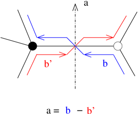
Figure 6: The charge of a link in the dimer in function of the weights $b$ of the zig-zag paths.

Let us restate more precisely the method to find the global charge of a link in the dimer in functions of the parameters $b_{i}$. Look at Figure 6: we orient the chiral field in the periodic quiver so that the white vertex of the dimer is on the right. With respect to this orientation of the chiral field the two zig-zag paths defining the link always arrive from the bottom and go out from the top of the link in the dimer. This is because the zig-zag paths always turn clockwise around white nodes and anticlockwise around black nodes (this is a consistency rule for the Fast Inverse Algorithm [9]). If $b$ is the weight of the zig-zag path entering at bottom right and going out at top left, and $b^{\prime}$ is the weight of the other zig-zag path entering at bottom left and going out at top right, then the global charge of the corresponding chiral field is always:

$$a=b-b^{\prime}$$ (5.2)

This is a precise reformulation of the algorithm in [34] that can be extended without ambiguities to all toric phases.

Note also that it is immediate to prove that rule (5.2) gives global non anomalous charges. The sum of the charges of the chiral fields connected to a node in the dimer is zero (invariance of the superpotential) since every zig-zag path appears twice in consecutive links, but its weight $b$ is once added and once subtracted. For the same reason the sum of global charges of links for every face of the dimer is zero (anomaly cancellation).

To find the baryonic charges we have to impose the constraint (2.4):

$$0=\sum_{i}a_{i}V_{i}=\sum_{i}b_{i+1}V_{i}-b_{i}V_{i}=\sum_{i}b_{i}(V_{i-1}-V_{i})$$ (5.3)

and since the difference $(V_{i-1}-V_{i})$ of consecutive vectors in the fan is proportional up to a rotation of $90^{o}$ to the vector $v_{i}$ of the (p,q) web, we find that the $d-3$ baryonic charges are those satisfying the constraints:

$$\sum_{i=1}^{d}b_{i}v_{i}=0$$ (5.4)

Note that equation (5.4) is identical to the conditions for having a first order deformation in Altmann’s construction [31].

Anomaly free rank distributions in the gauge theory can therefore be built from assignments of weights $b(v)$ to all vectors $v$ in the (p,q) web satisfying equation (5.4).

Consider the case when the toric CY cone has a $k-1$ dimensional branch of complex structure deformations, that is the toric diagram $P$ admits a Minkowski decomposition into $k$ polytopes $P=P_{1}+\ldots P_{k}$. Recall that the set of sides of $P$ is the union of the set of sides of the summands $P_{j}$: equivalently the set of vectors $v$ of the (p,q) web is split into $k$ disjoint subsets of vectors (let us call these sub-webs again $P_{j}$) at equilibrium, that is for every sub-web $P_{j}$ the sum of vectors is still zero. As explained in Section 3, we expect the existence of a fractional brane (rank distribution in field theory) dual to a supergravity solution with a smoothed deformed cone. We propose the following conjecture for finding such rank distribution:

Deformation Fractional Branes: The rank distribution in the quiver gauge theory dual to the deformation of a toric CY cone with toric diagram $P=P_{1}+\ldots P_{k}$ is computed through a baryonic charge obtained assigning constant weights $M_{j}$ to all the vectors belonging to the same sub-web $P_{j}$: $b(v)=M_{j}$ for $v\in P_{j}$, $j=1,\ldots k$.

Note in fact that since sub-webs are in equilibrium, equation (5.4) is trivially satisfied, and the rank distribution will be anomaly free. This proposal nicely fits Altmann’s rule of decomposition into a Minkowski sum. The rank distribution depends on $k$ arbitrary constants $M_{j}$, but indeed the parameter space of deformations is $k-1$ dimensional: recall that adding a common constant to all weights $b$ in the (p,q) web does not change the baryonic symmetry, so that fractional branes are indeed counted by the differences between the constants $M_{j}$. Correspondingly in the gauge theory the rank distribution is defined up the a common constant that can be added to all gauge groups (regular branes).

We have not a general proof of the above proposal, but we checked it in many concrete examples. One important check that one can perform is that rank distributions computed with the above proposal lead to a supersymmetric vacuum. In the case where a single deformation parameter is turned on, it is easy to prove that with the proposed rank distributions no gauge group develops an ADS superpotential and therefore the vacuum is expected to be supersymmetric, see the following Section. A more refined check is to compute the moduli space of the quiver gauge theory, probed by a single regular brane $N=1$, and show that it is the deformed cone. We will do this on a concrete example in Section 8 along the lines of [33, 26], but after having introduced the useful tool of the $\Psi$-map.

We point out that in general there can be different rank distributions on the same dimer configuration (also having fixed the toric phase), that are dual to the same deformed geometry with the same deformation parameters. For instance consider the splitting of the (p,q) web in only two sub-webs at equilibrium: the distance between their weights $b$ is an integer $M$, (number of fractional branes). By changing $M$ in $-M$ we find another distribution of ranks for gauge groups, that could seem also very different from the previous one. But in all the examples we considered we found that after applying some Seiberg dualities it is possible to pass from one distribution to the other and hence they describe the same deformed geometry (in fact analyzing the two cascades in the far IR with a single regular brane one can see that they reduce to the same theory). We suggest that this is a general feature.

Another possible ambiguity arises when the singularity is not isolated. In this case there are parallel vectors in the (p,q) web perpendicular to the same edge of the toric diagram. If the toric diagram has a Minkoswki decomposition, the assignments of this parallel vectors in the (p,q) web to the different sub-webs may be ambiguous, and this gives rise to apparently different rank distributions (look at Figure 3 and at the two baryonic charges in Figures 8 a) and b)). However the Minkowski decomposition into polytopes is the same and we expect a unique deformation; again we checked in the considered examples that these ambiguities are resolved by Seiberg dualities: also in these cases the different rank distributions are connected by Seiberg dualities. Therefore we conjecture that all baryonic symmetries with weights constant on sub-webs in equilibrium compute rank distributions dual to deformed geometries, but what matters are the absolute distances between the weights of the sub-webs.

Let us now turn to the case of $\mathcal{N}=2$ fractional branes. Consider a toric diagram with one edge $E$ having $k-1$ integer internal points (see Figure 7 for the case $k=4$). This corresponds to a surface of singularities of $\mathbb{C}^{2}/\mathbb{Z}_{k}$ type. In the (p,q) web there are $k$ vectors $w_{1},\ldots w_{k}$ perpendicular to the edge $E$. Our proposal is:

$\mathcal{N}=2$ fractional branes: The rank distributions in the quiver gauge theory corresponding to $\mathcal{N}=2$ fractional branes are computed by baryonic symmetries obtained assigning weights $b(w_{j})=b_{j}$, $j=1,\ldots k$ for the $k$ vectors $w_{j}$ perpendicular to $E$ with the constraint $b_{1}+\ldots b_{k}=0$, and $b(v)=0$ for all other vectors $v$ in the (p,q) web.

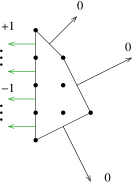
Figure 7: The weights $b_{i}$ for $\mathcal{N}=2$ branes.

Again recall that we can add a common constant to all $b_{i}$ of these configurations and have still the same baryonic symmetry, and hence the same rank distribution. Note that this choice obviously satisfies equations (5.4) for baryonic charges since we have imposed that the sum of weights $b_{j}$ is zero. Moreover there is a space of $k-1$ independent $\mathcal{N}=2$ fractional branes as expected for $\mathbb{C}^{2}/\mathbb{Z}_{k}$ singularities. Only parameters $a_{i}$ associated with integer points along the edge $E$ or with its vertices are different from zero. We will check this assignment on concrete examples in the following subsection.

To conclude we suggest that different assignments of baryonic charges, not associated with splittings of (p,q) web or with edges with integer points, correspond in general to SB fractional branes.

6 Examples and further observations

Let us start with the example of the SPP. It has $d=5$ and hence has a two dimensional space of fractional branes, but only a one dimensional space of complex deformations. It is known in the literature that the rank distribution $(N,N+M,N)$ for gauge groups (1,2,3) reported in Figure 2, corresponds to a deformation brane. In fact it is easy to see from Figures 1 and 2 that this corresponds to the choice of baryonic charges $(a_{1},a_{2},a_{3},a_{4},a_{5})$ = $(-M,M,-M,M,0)$ or equivalently $(b_{1},b_{2},b_{3},b_{4},b_{5})$ =$(M,0,M,0,M)$. These charges are reported in Figure 8 a), from which it is evident that the weights $b$ for sub (p,q) webs in equilibrium are constant. The gauge theory undergoes a cascade of Seiberg dualities that reduce the number of regular branes $N\rightarrow N-M$. In the IR, if there are no more regular branes (that is $M$ divides $N$) we can put $N=0$ and so only a single confining $SU(M)$ gauge group survives (the second one). This is the case $M>0$.

If instead $M$ is negative, in the IR we have to put $N=|M|$ and we get two $SU(|M|)$ gauge groups (groups 1 and 3, whereas groups 2 disappears) and a superpotential term $W_{0}=-X_{11}X_{13}X_{31}$. By performing a Seiberg duality with respect to face 3 (the square) we come back to a single isolated gauge group.

There is another equivalent distribution of ranks corresponding to the deformation brane: $(b_{1},b_{2},b_{3},b_{4},b_{5})$ = $(0,M,0,0,M)$; this is reported in Figure 8 b): it corresponds again to a subdivision into two subwebs in equilibrium. The rank distribution corresponding to this baryonic symmetry is $(N,N,N+M)$. Since the exchange of gauge groups 2 and 3 is a symmetry of this theory (look the dimer from upside down) it is easy to see that this gauge theory is equivalent to the previous one. Again M can be also negative.

Since SPP is not an isolated singularity, there is also an $\mathcal{N}=2$ fractional brane: it is known that the associated rank distribution for the gauge groups is $(N+M,N,N)$, and this corresponds to the choice of baryonic charge $(b_{1},b_{2},b_{3},b_{4},b_{5})$ = $(0,0,0,M,-M)$, in agreement with our proposal.

In Figure 8 d) we report a choice of baryonic charges that gives the rank distribution: $(N+M,N,N+2M)$. For this type of fractional brane a supersymmetric vacuum is not present: group 3 has $N_{f}<N_{c}$ (with N=0) and generates a non perturbative ADS superpotential leading to runaway behavior. The corresponding baryonic symmetry $b_{i}:$ $(0,2M,0,M,M)$ is not associated with a splitting of the (p,q) web in subwebs at equilibrium. Note that this configuration can be obtained as a linear combination of the two deformation branes in Figure 8 a) and 8 b) up to a global constant for all $b_{i}$: generic superpositions of fractional deformation branes that do not satisfy the criterion in Section 5 lead to SB. This fact was already noted in [25].

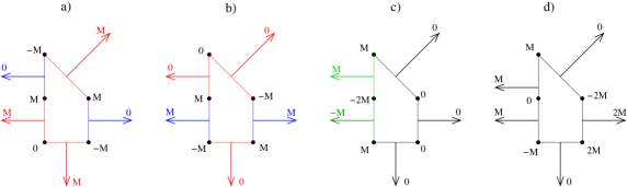
Figure 8: The weights for baryonic charges in SPP theory. a) Deformation brane; rank distribution: $(N,N+M,N)$. b) Deformation brane; rank distribution: $(N,N,N+M)$. c) $\mathcal{N}=2$ brane; rank distribution $(N+M,N,N)$. d) SB brane; rank distribution: $(N+M,N,N+2M)$.

Consider now the general case when the (p,q) web is splitted into two different sub-webs $P_{1}$ and $P_{2}$ at equilibrium (if further splittings are allowed we turn on a single deformation parameter). According to our proposal the deformational fractional brane is computed by a baryonic symmetry with weights $b$ of the type: $b(v)=-M$ if $v\in P_{1}$, $b(v)=0$ if $v\in P_{2}$. Look at Figure 9, where for simplicity $P_{1}$ is a triangle.

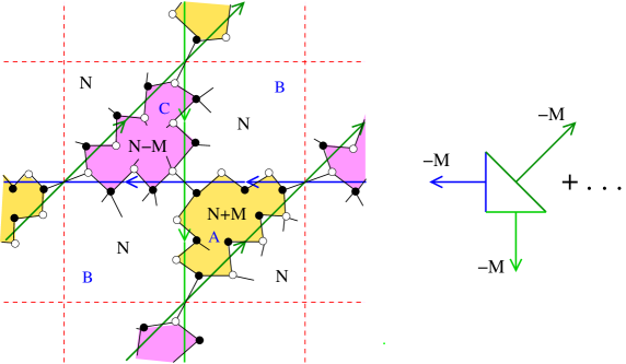
Figure 9: The rank distribution for a gauge theory dual to a toric geometry obtained by the Minkowski sum of a triangle and another polygon. More generally if there is only one deformation parameter the gauge groups can be only $SU(N)$, $SU(N+M)$ and $SU(N-M)$.

To reconstruct the dimer we have to draw the zig-zag paths corresponding to vectors of $P_{1}$ and $P_{2}$ as in [9], with the suitable consistency conditions. It is interesting to note that in the complete dimer for $P_{1}+P_{2}$, the zig-zag paths corresponding to $P_{1}$ (or $P_{2}$) satisfy separately the consistency conditions: for example in Figure 9, if we isolate the three zig-zag paths associated with vectors of $P_{1}$ (lines in light green, dark green and blue) we see that they divide the fundamental cell of the torus (delimited by the red dashed lines) into three regions: a face (in magenta) where the zig-zag paths turn clockwise, another face (in yellow) where the zig-zag paths turn anticlockwise, and a third face with an even number of sides (where zig-zag paths are not oriented). This is just the way in which the Fast Inverse Algorithm reconstructs the theory associated with the triangle $P_{1}$, the $\mathcal{N}=4$ SYM: the non oriented face is the gauge group, clockwise oriented face is the white vertex, and anticlockwise oriented face is the black vertex.

This is a general feature of dimers dual to a toric diagram that can be splitted in $P_{1}+P_{2}$ and has been recently noted also in [32], where it was explained in the context of mirror symmetry and using ideas from geometric transition.

For a generic polytope $P_{1}$ we will call $C$ ($A$) the regions along which zig-zag paths of $P_{1}$ turn clockwise (anticlockwise) and $B$ the non-oriented regions. In general $A$, $B$, $C$ are unions of contractible regions in the torus $T^{2}$; a region of type $A$ (or $C$) is rounded only by region(s) of type $B$.

In Figure 9 we have drawn only the zig-zag paths associated with $P_{1}$; their intersections correspond to links in the dimer that separate regions of type $B$ and have baryonic charge zero. But there are other links: we have drawn also all the links of the dimer along the zig-zag paths of $P_{1}$: they correspond to an intersection of a zig-zag paths of $P_{1}$ with one of $P_{2}$. Note that inside the regions $C$ ($A$) there are only white (black) vertices belonging to the zig-zag paths of $P_{1}$ because zig-zag paths turn clockwise (anticlockwise) around white (black) nodes; there could be however “more interior” vertices of different colors inside $C$ and $A$, not belonging to the zig-zag paths of $P_{1}$.

The links in the dimer correspond to intersections of two zig-zag paths: if the zig-zag paths are associated with (p,q) web vectors of the same sub-web $P_{i}$, then the baryonic charge of the link is zero because of equation (5.2), otherwise the charge is $M$ or $-M$. Therefore the only charged links under the baryonic symmetry are those separating regions of type $A$ from regions of type $B$ and regions $C$ from $B$. Let us assign number of colors $N$ to all faces in regions $B$; then using the rules and the conventions explained in Section 5 and in Figure 6 we can deduce that all faces in regions $A$ will have number of colors $N+M$ and regions $B$ number of colors $N-M$.

So our proposed baryonic symmetry gives rise only to gauge groups $SU(N)$, $SU(N+M)$ or $SU(N-M)$ (one of these could be absent as we will see). If we suppose the existence of a cascade, in the IR (when $M$ divides $N$), we can put $N=M$. At this step all regular branes have disappeared and we have only gauge groups $SU(M)$ in regions $B$ and $SU(2M)$ in regions $A$. These gauge groups cannot develop ADS terms: since $N_{f}$ and $N_{c}$ are both multiples of $M$ the only problem would be an $SU(2M)$ gauge group with $M$ flavors. But region $A$ is rounded by region $B$ and so an $SU(2M)$ gauge group is rounded at least by four faces (it is at least a square) with colors at least $SU(M)$, therefore it has $N_{f}\geq 2M$. Obviously ADS terms cannot appear in previous steps of the cascade: if we add regular branes (in multiples of $M$) then for every gauge group $N_{f}$ increases faster than $N_{c}$.

Since no ADS term is generated we expect in these cases that supersymmetry is not spontaneously broken. In concrete examples we found that, also when regular branes have disappeared, it is possible to continue to perform some Seiberg duality (gauge group condensation) until we are left with only isolated confining gauge groups.

If for example there are no faces in regions $C$ (no $SU(N-M)$ gauge groups) the analysis is easier: in the IR we can put N=0, so that we are left only with $SU(M)$ gauge groups in regions $A$. Again there are no ADS superpotential terms ($N_{f}=0$ or $N_{f}\geq M$). Note that superpotential terms due to vertices inside regions $A$ typically allow to perform gauge condensations until only confining groups and no massless chiral matter survives in the IR.

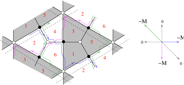
Figure 10: The rank distribution for deformation of $dP_{3}$, corresponding to Figure 4 a). The shadowed gauge groups 1,3 and 5 are $SU(N+M)$. The other groups, 2,4,and 6, are $SU(N)$.

We can check these ideas in the known case of $dP_{3}$ [24, 25]. For the first deformation branch in Figure 4 a) we draw the rank distribution in Figure 10, where we show the three zig-zag paths corresponding to the edges of one of the triangles in the Minkowski sum of the toric diagram. Note that in this case the region of type $C$ contains only a white vertex and no faces, so that there are only $SU(N)$ gauge groups (faces 2,4,6 in regions $B$) and $SU(N+M)$ gauge groups (faces 1,3,5 in region $A$). In the IR we can put $N=0$ and we have the three $SU(M)$ gauge groups 1,3,5 with the corresponding superpotential term. Performing a Seiberg duality (gauge group condensation on the baryonic branch) with respect to one of them and integrating out massive fields we have two confining gauge groups in the IR.

Other cases with a single deformation parameter $P=P_{1}+P_{2}$ that have only $SU(N)$ and $SU(N+M)$ gauge groups are the cases where $P_{1}$ is a segment: the (p,q) web of $P_{1}$ is a pair of opposite vectors, see Figure 15 below.

We give a concrete example of the general case in Figure 11: we consider a toric diagram $P$ obtained by summing the toric diagram of $P_{1}\equiv\mathbb{C}^{3}$ (a triangle) and of $P_{2}\equiv Y^{2,1}$. We constructed a minimal toric phase, reported in Figure 11, with the Fast Inverse Algorithm [9]. There are $11$ gauge groups labelled in red; the red dashed lines delimit the fundamental cell. You can see that assigning weights $b_{i}$: $(0,-M,0,-M,0,-M,0)$ to the zig-zag paths we obtain the rank distribution for the fractional deformation brane reported in Figure 11 with $SU(N+M)$ for faces 9,4 (type $A$ regions); $SU(N-M)$ for face 11 (type $C$ region), and $SU(N)$ for the remaining gauge groups.

Note that since this is not an isolated singularity we have the ambiguity described it the previous Section: we can assign also weights $b_{i}$: $(-M,0,0,-M,0,-M,0)$ and obtain an equivalent rank distribution with only $SU(N-M)$ and $SU(N)$ gauge groups. We report the possible rank distributions for this theory in the following table:

$$\small\begin{array}[]{c|ccccccccccc}(b_{1},b_{2},b_{3},b_{4},b_{5},b_{6},b_{7})&1&2&3&4&5&6&7&8&9&10&11\\[4.5pt] \hline\cr(0,-M,0,-M,0,-M,0)&N&N&N&N+M&N&N&N&N&N+M&N&N-M\\ (-M,0,0,-M,0,-M,0)&N&N&N&N&N-M&N-M&N&N-M&N&N-M&N-M\\ (0,M,0,M,0,M,0)&N&N&N&N-M&N&N&N&N&N-M&N&N+M\\ (M,0,0,M,0,M,0)&N&N&N&N&N+M&N+M&N&N+M&N&N+M&N+M\end{array}$$

where we have added in the last two lines also the possibilities of exchanging $M$ with $-M$, (in the following: $M>0$).

The four distributions above may seem at first glance to be different; indeed we checked for all of them the existence of a cascade of Seiberg dualities: the dimers come back to themselves up to a permutation of groups with $N\rightarrow N-M$. At the end of the respective cascades we find (if $M$ divides $N$) that gauge groups condensate until there remain always three isolated confining gauge groups. If instead we consider the case with one regular brane remaining in the IR (like in Section 8) the four gauge theories reduce to the same theory in the IR, so that they are dual to the same deformed geometry. More generally it is possible to find Seiberg dualities that send each configuration in the previous table to one another.

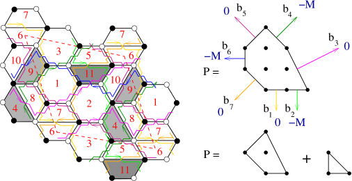
Figure 11: Dimer configuration dual to the toric diagram $P=Y^{2,1}+\mathbb{C}^{3}$.

Deformations with more parameters are in general more difficult to treat. In Figure 12 we report the rank distribution for the deformation of the cone over $dP_{3}$ corresponding to Figure 4 b). This is a two parameters branch and correspondingly we have two integers, $P$ and $M$ parametrizing the weights for the zig-zag paths: $b_{i}=$ $(P,P+M,M,P,P+M,M,P)$. Note that our proposal for the baryonic charge of deformation branes reproduces the known results in the literature, see Figure 12 b).

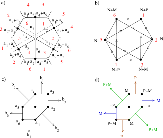
Figure 12: The deformation of $dP_{3}$ corresponding to Figure 4b). a) Dimer configuration and distribution of charges. b) Quiver and rank assignment. c) Toric Diagram. d) Values of $a_{i}$ and $b_{i}$ for the baryonic charge corresponding to this rank distribution.

Figure 13: The quiver gauge theory for $dP_{3}$ in the IR with only fractional branes, corresponding to Figure 12 b).

In the IR, when all regular branes have disappeared ($N=0$), there remain the four gauge groups $1,3,4,6$ with ranks respectively $P,M,P,M$, see Figure 13, and the tree level superpotential term:

$$W_{0}=-\mathrm{tr}\left(X_{61}X_{13}X_{34}X_{46}\right)$$ (6.1)

differently from the case with a single deformation parameter, we see that ADS superpotential terms may appear. In our example, if $P>M>0$, groups 1 and 4 have $N_{f}<N_{c}$ and so the superpotential becomes,

$$W=-\mathrm{tr}\left(M_{63}M_{36}\right)+c\left(\frac{1}{\mathrm{det}M_{63}}\right)^{\frac{1}{P-M}}+d\left(\frac{1}{\mathrm{det}M_{36}}\right)^{\frac{1}{P-M}}$$ (6.2)

where $M_{63}$ and $M_{36}$ are the $M\times M$ mesonic matrices of groups $1$ and $4$ respectively. It is easy to see that F-term and D-term equations can be satisfied (choose the meson matrices proportional to the identity). Therefore there exists a supersymmetric vacuum for this theory.

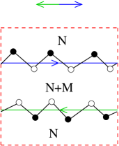
Figure 14: Rank distribution for a fractional deformation brane obtained by lifting a subweb made up of two opposite vectors.

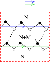
Figure 15: Rank distribution for an $\mathcal{N}=2$ fractional brane obtained by giving opposite weights to two (p,q) web vectors perpendicular to the same edge of the toric diagram.

Let us now make some further comments on the $\mathcal{N}=2$ fractional branes. In Figures 15, 15 we compare the case of a fractional deformation brane obtained by lifting two opposite vectors in the (p,q) web with the same weights (Figure 15), and the case of an $\mathcal{N}=2$ fractional brane obtained by giving opposite weights to two parallel vectors in the (p,q) web (perpendicular to the same edge of the toric diagram), and weight zero to all other vectors. In both cases the fundamental cell of the torus (delimited by the red dashed lines in the Figures) is divided in two strips where faces have ranks $N$ and $N+M$ respectively. We have drawn only the white and black vertices belonging to the two zig zag paths we are considering: for the deformation brane inside the strip with $N+M$ ranks there fall the white vertices: one would need an even number of links to pass from one white vertex of the first zig-zag path to a white vertex of the second zig-zag path; among these configurations there are also those consisting of only isolated groups. Instead for the $\mathcal{N}=2$ fractional brane, inside the strip with $N+M$ ranks there fall the white vertices of the first zig-zag path and the black ones of the second zig-zag path: now an odd number of links is required to pass from one set of vertices to the other. Consider for example the $\mathcal{N}=2$ fractional brane obtained with $b_{1}=M$ and $b_{2}=-M$ in Figure 11, and zero to the remaining $b_{i}$. If we do not insert regular branes ($N=0$), we have a closed loop of $SU(M)$ gauge groups connected by chiral fields (faces 6,5,4,8,9,10) but with no superpotential term. If we give vev to all but one chiral fields the theory reduces to a single gauge group with an adjoint multiplet.

The analysis just performed fits the observation already done in [25] that $\mathcal{N}=2$ fractional branes correspond to rank distributions where faces with $N+M$ rank form parallel strips on the torus: this is due to the fact that we give weights only to parallel vectors in the (p,q) web, that correspond to parallel not intersecting zig-zag paths.

In Figure 16 we give a more complicated example of an $\mathcal{N}=2$ fractional brane: the theory is $L^{2,3;3,2}$ whose dimer and toric diagram are reported in Figure 16 a) and b) respectively. We draw in the dimer only the three zig-zag paths that correspond to the vectors perpendicular to the fourth edge of the toric diagram. You can check that giving weights that sum up to zero only to these three vectors you obtain theories that have regions of the moduli space with an accidental $\mathcal{N}=2$ supersymmetry. For instance if we give weights $(-M,-M,2M)$ we obtain the rank distribution $(N,N+M,N+M,N+2M,N+2M)$ for the five gauge groups. If there are no regular branes $N=0$, the quiver reduces to that drawn in Figure 16 c) with the superpotential:

$$W=X_{23}X_{34}X_{43}X_{32}-X_{45}X_{54}X_{43}X_{34}$$ (6.3)

Giving vev to, for instance, $X_{23}$ and $X_{45}$ and integrating out massive fields the quiver reduces to that reported in Figure 16 d): there are two gauge groups with adjoints and an hypermultiplet of $\mathcal{N}=2$. Also the superpotential (6.3) reduces to that of an $\mathcal{N}=2$ theory with matter.

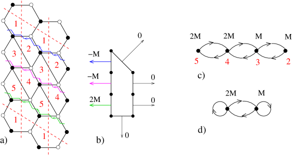
Figure 16: $\mathcal{N}=2$ fractional branes in the theory for the cone over $L^{2,3;3,2}$. a) Dimer configuration. b) Toric diagram and weights for the baryonic symmetry. c) Quiver gauge theory (with $N=0$). d) Quiver after giving vevs to $X_{23}$ and $X_{45}$.

7 Comments on the $\Psi$-map

In this Section we introduce the correspondence between the chiral ring of mesonic operators in the (superconformal) field theory and the semigroup of integer points in $C^{*}$, the dual cone of the fan $C$. This correspondence has already been studied in the literature [21, 12], see also [41]; here we simply translate these results in the language of charges and zig-zag paths. Then we provide a direct proof in field theory that the $\Psi$-map of a mesonic operator is an affine function, and make further useful comments.

The idea of the correspondence is simple: the moduli space of a superconformal quiver gauge theory (we can restrict to the abelian case $N=1$ with a single regular brane) is the toric CY cone where the D3-brane can move in the string theory set up; this toric cone is described by a convex rational polyhedral cone in $\mathbb{R}^{3}$, the fan $C$. Mesonic operators (closed oriented loops) in field theory can be considered as well defined functions on the toric cone: the value of the function in every point of the moduli space is the vev of the mesonic operator in that vacuum. Obviously such functions are the same for F-term equivalent operators. In toric geometry the ring of algebraic functions on the toric cone is in one to one correspondence with the semigroup of integer points in $C^{*}$, the dual cone of the fan $C$ (generated by inward pointing normals to the faces of $C$).

$$C^{*}=\{x\in\mathbb{R}^{3}\,|\,(x,y)\geq 0\quad\forall y\in C\}$$ (7.1)

We may then expect a one to one correspondence between the chiral ring of mesonic operators, equivalent up to F-terms, and the integer points in $C^{*}$. This is indeed the case, and, as we will see, the three integer numbers that are associated to mesons are (related to) the charges of the meson under the three global $U(1)$ isometries of the geometry, that are the flavor symmetries and the R-symmetry in field theory. A precise mapping can be obtained using the $\Psi$-map, introduced in [21].

Let us consider an oriented link $X$ in the periodic quiver (or in the dimer). As explained in Sections 2.1 and 5, one can parametrize the charges of the link $X$ with a formal expression:

$$\Psi(X)=\sum_{i=1}^{d}c_{i}a_{i}$$ (7.2)

where the coefficients $c_{i}$ are integer numbers (0 or 1 for a single link) that can be easily computed using one of the two algorithms reviewed in Section 2.1. The $\Psi$-map associates to every oriented link $X$ a function $\Psi(X)$ defined on the vertices (and integer points on the boundary) of the toric diagram $P$ of the dual geometry. This function evaluated at vertex $i$ is defined as: $\Psi_{i}(X)=c_{i}$. In the following we shall use the same expression $\Psi(X)$ for this function and for the expression in (7.2).

As in [21] we linearly extend the $\Psi$ map to the group of one-chains $L$ in the periodic quiver, the free group generated by the oriented links $X_{j}$ in the quiver with integer coefficients:

$$L=\sum_{j}d_{j}X_{j}\qquad d_{j}\in\mathbb{Z}$$ (7.3)

In particular the $\Psi$ map of a path in the quiver is obtained by summing the trial charges of fields in the path (or by subtracting the charges for links that are not oriented in the same direction as the path).

Note that this definition is equivalent to that given in [21]: for a path $L$, $\Psi_{i}(L)$ is the number of intersections (weighted with +1 or -1 according to orientation) of $L$ with the perfect matching in the dimer corresponding to the $i$-th vertex of the toric diagram. This intersection number is just the coefficient $c_{i}$ of $a_{i}$ in the expression of the $\Psi$-map for $L$: $\Psi(L)=\sum_{i}c_{i}a_{i}$, according to the algorithm in [15] for distributing charges.

Note that, for non isolated singularities, it is possible to extend the function $\Psi(X)$ to all the integer points along the boundary of the toric diagram (this can be done unambiguously using the algorithm in [34] for distributing charges, in particular using the conventions in (5.1) and (5.2)).

Let us fix a system of coordinates for the fan $C$, such that the generators have third coordinate equal to one: the integer points along the boundary of the toric diagram are: $V_{i}=(x_{i},y_{i},1)$, $i=1,\ldots d$. This defines the linear functions $x$ and $y$ in the plane of the toric diagram. As already observed in [21, 12], the $\Psi$-map of a closed loop $L$ in the periodic quiver is an affine function:

Theorem 7.1

If $L$ is a closed loop of chiral fields (oriented or not), then the $\Psi$-map for $L$ is:

$$\Psi(L)=\sum_{i=1}^{d}\left(nx_{i}+my_{i}+c\right)a_{i}$$ (7.4)

where $(n,m,c)$ are integer numbers and $(n,m)$ are the homotopy numbers of the loop $L$ on the torus $T^{2}$ of the periodic quiver or dimer.

We give here a simple proof of this statement. From the definition (7.2) it is obvious that the $\Psi$-map of any one cycle is a homogeneous degree-one polynomial in the $d$ variables $a_{i}$. We may then restrict to the $d-1$ global charges imposing the constraint (2.3) and prove that for a closed loop: $\Psi(L)=\sum_{i=1}^{d}\left(nx_{i}+my_{i}\right)a_{i}$. Then the general case can only differ from this expression for an integer constant $c$ times the sum of all $a_{i}$. Now if (2.3) holds we can parametrize the global charges as in Section 5 using the parameters $b_{i}$ associated with zig-zag paths and related to $a_{i}$ through (5.1). The charge of a generic link can be computed as in (5.2): as shown in Figure 6 we have to add the weight $b$ if the topological intersection between L and the zig-zag path is $+1$ or subtract the weight $b$ if the intersection is $-1$. Let us call $w\equiv(n,m)$ the homotopy numbers of the loop L on the torus $T^{2}$; the homotopy numbers of the zig-zag paths are given by the vectors $v_{i}$ of the (p,q) web, $v_{i}=(p_{i},q_{i})$. The topological intersection between $L$ and the $i$-th zig-zag path is $\mathrm{det}(w,v_{i})$, and summing them with the weights $b_{i}$ we get the global charge of $L$:

$$\Psi(L)=\sum_{i=1}^{d}\mathrm{det}\left(w,v_{i}\right)\,b_{i}\qquad\mathrm{if}\quad\sum_{i=1}^{d}a_{i}=0$$ (7.5)

Note that this is true also if the links in $L$ are not all oriented in the same direction. If $\tilde{V}_{i}\equiv(x_{i},y_{i})$ are the coordinate vectors of the integer points along the perimeter of the toric diagram, the vectors $v_{i}$ can be obtained by a $90^{o}$ rotation of the edges of the toric diagram:

$$v_{i}=R\left(\tilde{V}_{i}-\tilde{V}_{i-1}\right)$$ (7.6)

where $R$ is the rotation matrix:

$$R=\left(\begin{array}[]{ll}0&1\\ -1&0\end{array}\right)$$ (7.7)

Indexes $i$ will be understood to be periodic of period $d$ and in our conventions are displaced as in Figure 5. Substituting (7.6) into (7.5) we compute:

$$\Psi(L) = \sum_{i}\mathrm{det}\left(w,\,R\tilde{V}_{i}\,b_{i}-R\tilde{V}_{i-1}\,b_{i}\right)$$ (7.8)

$$= \sum_{i}\mathrm{det}\left(w,R\tilde{V}_{i}\,(b_{i}-b_{i+1})\right)$$

$$= -\sum_{i}\mathrm{det}\left(w,R\tilde{V}_{i}\right)a_{i}$$

$$= \sum_{i}(nx_{i}+my_{i})\,a_{i}\qquad\qquad\quad\mathrm{if}\quad\sum_{i=1}^{d}a_{i}=0$$ (7.9)

where in the third equality we have used the relation (5.1). This concludes the proof. Note as a particular case that equality (7.8) together with (2.4) also shows that the baryonic charge of a closed loop is zero, as claimed in Section 4.

Mesonic operators in field theory are the trace of chiral fields along an oriented closed loop $L$. In the oriented case the coefficients $d_{i}$ in (7.3) are all non negative, and hence the coefficients $c_{i}$ in $\Psi(L)=\sum_{i}c_{i}a_{i}$ are all non negative. Because of theorem (7.1) the $c_{i}$ are the scalar products:

$$c_{i}=\left((n,m,c),(x_{i},y_{i},1)\right),\qquad\qquad c_{i}\geq 0\,\,\,\mathrm{for}\,\,\mathrm{oriented}\,\,\mathrm{loops.}$$ (7.10)

We see therefore that the vector $(n,m,c)$ lies in $C^{*}$ for mesons. Hence the explicit mapping from mesons to integer points in $C^{*}$ is just given by the $\Psi$-map (7.4): $L\leftrightarrow(n,m,c)$.

Note that this correspondence is well defined under changes of coordinates: the coefficients $c_{i}$ of the $\Psi$-map (7.2) do not depend on the choices of coordinates, hence if we perform a translation or an $SL(2,\mathbb{Z})$ transformation of the toric diagram, the point $(n,m,c)$ transforms as a point of the dual lattice $C^{*}$ to keep the scalar product $c_{i}$ in (7.10) constant.

Since F-term equivalent mesons have the same charges they are mapped to the same point $(n,m,c)$. Conversely if mesons are mapped to the same point $(n,m,c)$ it means that they have the same homotopy numbers in the torus and the same “length” (i.e. the same R-charge in the language of [21], this is obvious since the $\Psi$-map is just a parametrization of the R-charge). Using Lemma 5.3.1 (that makes use of the hypotheses of consistency of the tiling) in [21] we conclude that such mesons are F-term equivalent. Moreover we suppose that the $\Psi$-map is surjective on $C^{*}$; the work of [21] also suggests that the correspondence is one to one.

As a consequence mesons in the chiral ring and integer points of the additive semi-group $C^{*}$ also satisfy the same algebraic relations: if two linear combinations with positive integer coefficients of integer vectors in $C^{*}$ are equal, then the composition of the corresponding mesons are still closed oriented loops with the same image under the $\Psi$-map, since it is linear, and are therefore $F$-term equivalent. Recall that in toric geometry to every independent generator of the semi-group $C^{*}$ is associated a complex variable $z_{j}$ and that linear relations between generators become equations that express the toric cone as a (non complete) intersection in the space of $z_{j}$. Conversely in field theory the moduli space (in the case with a single regular brane $N=1$) can be computed through algebraic and F-term relations between mesonic operators (for concrete examples see the following Section or the work of [33]). We have just seen through the $\Psi$-map that the two kinds of computations always agree in the toric superconformal case: a consistent dimer configuration built according to the rules of the Fast Inverse Algorithm [9] has a moduli space of vacua that always reproduces the dual toric geometry. Therefore we point out that the $\Psi$-map theory can work as an argument to show directly that the Fast Inverse Algorithm is correct. In fact the proofs of disposition of charges, of Theorem 7.1, and of Lemma 5.3.1 in [21] are based only on the assumption that the dimer is built according to the rules of the Fast Inverse Algorithm: zig-zag paths must be closed non intersecting loops, they are in one to one correspondence with the legs of the (p,q) web and must be drawn on a torus with the homotopy numbers (p,q) of the corresponding leg; links in the dimer are in one to one correspondence with intersections of two zig-zag paths; zig-zag paths turn clockwise around white vertices and anticlockwise around black vertices…

In the following Section we shall see how the $\Psi$-map works on a concrete example; moreover the $\Psi$-map greatly simplifies the problem of finding the mesons corresponding to generators of $C^{*}$. Then we shall consider the deformed moduli space in presence of fractional branes. To conclude we note that the vector $(0,0,1)$ always belongs to $C^{*}$ since the generators $V_{i}$ are $(x_{i},y_{i},1)$. This vector will play an important role in the study of deformations. In the superconformal case the mesons that are mapped to this vector are the superpotential terms (recall that their R-charge is 2, and hence their $\Psi$ map is $\sum_{i}a_{i}$); they are all F-term equivalent as it is easy to prove directly or using the fact that they are mapped to the same vector under $\Psi$-map.

8 Computing the deformed geometry: a detailed example

Up to now we have checked in examples that our prescription in Section 5 for fractional deformation branes leads to a supersymmetric vacuum: in the IR if no regular branes survive after the cascade we find isolated confining gauge groups. Indeed one should check that also the deformed geometry is reproduced by the gauge theory. We will do that on a specific example, along the lines of [33], by considering the case of a single regular D3 brane in the IR, plus the fractional branes. The moduli space of the gauge theory, deformed by the presence of ADS terms, describes the geometry probed by the D3 brane and therefore should match with the geometry of the deformed cone that can be computed through Altmann’s algorithm [31].

The example we have chosen is the $PdP_{4}$ theory, whose toric diagram has vertices:

$$(0,0,1)\quad(2,0,1)\quad(2,1,1)\quad(1,2,1)\quad(0,2,1)$$ (8.1)

and admits a Minkowski decomposition into a triangle and two segments, see Figure 17, corresponding to a two dimensional deformation branch.

Figure 17: The toric diagram for the cone over $PdP_{4}$ and its Minkowski decomposition.

The dimer can be easily reconstructed through the Fast Inverse Algorithm or by looking in the literature: we report it in Figure 18, where we draw also the zig-zag paths and their correspondence with vectors in the (p,q) web. This is a minimal toric phase. There are $7$ gauge groups labelled in red: we have chosen this labelling so as to reproduce the quiver in Figure 15 of [25]. The fundamental cell is delimited by the dashed black lines in the dimer. From the zig-zag paths it is easy to reconstruct the charge distribution for links in the dimer, as explained in Sections 2.1 and 5; we draw it in Figure 19.

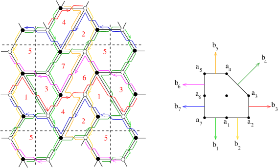
Figure 18: The dimer configuration for $PdP_{4}$. We report on the right also the toric diagram for $PdP_{4}$ with the legs of the (p,q) web colored as the corresponding zig-zag paths in the dimer.

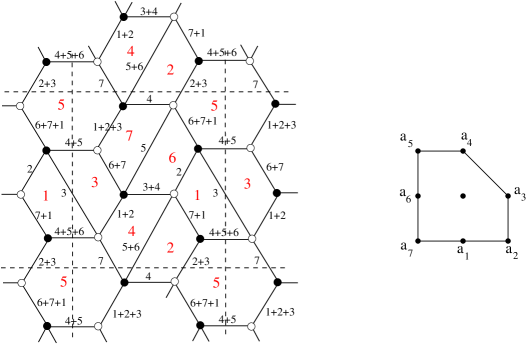
Figure 19: The distribution of charges $a_{i}$ for $PdP_{4}$. In the dimer a black number $i$ near a link stands for the charge $a_{i}$.

Let’s start with the superconformal case. First of all we have to compute the cone $C^{*}$: the inward pointing perpendiculars to the faces of (8.1) are:

$$z_{1}\rightarrow(0,1,0)\quad z_{2}\rightarrow(-1,0,2)\quad z_{3}\rightarrow(-1,-1,3)\quad z_{4}\rightarrow(0,-1,2)\quad z_{5}\rightarrow(1,0,0)$$ (8.2)

they are primitive integer vectors. These vectors generate $C^{*}$ over $\mathbb{R}^{+}$, but do not generate the lattice cone of integer points in $C^{*}$ over positive integer numbers. In our case we have to add another generator:

$$t\rightarrow(0,0,1)$$ (8.3)

We assign complex variables $z_{1}$, $z_{2}$, $z_{3}$, $z_{4}$, $z_{5}$, $t$ to the six generators as in (8.2) and (8.3).

Linear relationships satisfied by the generating vectors (linear combination with positive integer coefficients equal to another combination with positive integer coefficients) are translated into complex equations for the corresponding variables. A minimal set of relations is in our case:

$$\begin{array}[]{lll}z_{1}z_{3}=z_{2}t&z_{2}z_{4}=z_{3}t&z_{3}z_{5}=z_{4}t\\ z_{2}z_{5}=t^{2}&z_{1}z_{4}=t^{2}&\end{array}$$ (8.4)

where for example the last equation translates the linear relation: $(0,1,0)$ $+$ $(0,-1,2)$ $=$ $2(0,0,1)$. The relations in (8.4) define the toric cone over $PdP_{4}$ as a non complete intersection in $\mathbb{C}^{6}$. Note in fact that there are 6 variables and 5 relations, but the cone has complex dimension 3: 2 relations depend on the others at generic points where $z_{i}$ and $t$ are not zero. In our example all generators lie on a plane (this is not true in general) and so it is simpler to find the relations.

To see that the moduli space of gauge theory (with $N=1$) reproduces the singular geometry (8.4), we have to compute the F-term relations in the chiral ring of mesonic operators.

To find mesons that correspond to the generating vectors of $C^{*}$, one can use the $\Psi$-map theory and Theorem 7.1 in Section 7. For example consider the first vector $z_{1}\rightarrow(0,1,0)$. We know that a meson $Z_{1}$ mapped to this vector by the $\Psi$-map has homotopy numbers given by the first two entries $(0,1)$, and $\Psi$-map equal to the linear function $y$ in the plane of the toric diagram, that is $\Psi(Z_{1})=\sum_{i}y_{i}a_{i}=a_{3}+a_{6}+2a_{4}+2a_{5}$ (look at Figure 18 for the disposition of $a_{i}$ in the plane of the toric diagram). So one can look for a path in the dimer or in the periodic quiver (drawn in Figure 20) with homotopy numbers $(0,1)$ of minimal length (adding loops would add factors of $\sum_{i}a_{i}$ to the $\Psi$-map). For example you can check that the meson $Z_{1}=X_{46}X_{67}X_{72}X_{24}$ has all these features and therefore it is $\Psi$-mapped to $(0,1,0)$, as one can check explicitly. Any other meson with the same $\Psi$-map is F-term equivalent.

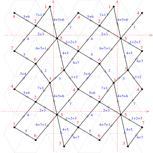
Figure 20: The periodic quiver for $PdP_{4}$. Red numbers label gauge groups, blue numbers label charges $a_{i}$.

Figure 21: The vectors $d_{j}$ for the toric diagram $PdP_{4}$.

Continuing in this way, one can find the following representatives for mesons corresponding to generating vectors:

$$\begin{array}[]{l|l|l|l|l}&(n,m,c)&nx+my+c&\Psi-\textrm{map}&\textrm{meson}\\ \hline\cr z_{1}&(0,1,0)&y&a_{3}+2a_{4}+2a_{5}+a_{6}&Z_{1}=X_{46}X_{67}X_{72}X_{24}\\ z_{2}&(-1,0,2)&-x+2&a_{1}+a_{4}+2a_{5}+2a_{6}+2a_{7}&Z_{2}=X_{35}X_{56}X_{67}X_{73}\\ z_{3}&(-1,-1,3)&-x-y+3&2a_{1}+a_{2}+a_{5}+2a_{6}+3a_{7}&Z_{3}=X_{45}X_{56}X_{67}X_{73}X_{34}\\ z_{4}&(0,-1,2)&2-y&2a_{1}+2a_{2}+a_{3}+a_{6}+2a_{7}&Z_{4}=X_{45}X_{57}X_{73}X_{34}\\ z_{5}&(1,0,0)&x&a_{1}+2a_{2}+2a_{3}+a_{4}&Z_{5}=X_{57}X_{72}X_{25}\\ t&(0,0,1)&1&a_{1}+a_{2}+a_{3}+a_{4}+a_{5}+a_{6}+a_{7}&T=X_{12}X_{25}X_{51}\end{array}$$ (8.5)

We understand the traces in writing mesons since when $N=1$ the fields are complex numbers. The superpotential $W_{0}$ can be read directly from the dimer:

$$W_{0} = X_{56}X_{67}X_{72}X_{25}+X_{73}X_{35}X_{57}+X_{46}X_{61}X_{12}X_{24}+X_{13}X_{34}X_{45}X_{51}$$ (8.6)

$$-X_{57}X_{72}X_{24}X_{45}-X_{13}X_{35}X_{56}X_{61}-X_{46}X_{67}X_{73}X_{34}-X_{51}X_{12}X_{25}$$

Using the F-term equations $\partial W_{0}/\partial X$ one can show that the mesons in (8.5) satisfy the same relations (8.4):

$$\begin{array}[]{lll}Z_{1}Z_{3}=Z_{2}T&Z_{2}Z_{4}=Z_{3}T&Z_{3}Z_{5}=Z_{4}T\\ Z_{2}Z_{5}=T^{2}&Z_{1}Z_{4}=T^{2}&\end{array}$$ (8.7)

In Section 7 we gave arguments based on the $\Psi$-map to show that this matching is true in general in the superconformal case.

Let us now consider the deformed case; we will start to compute the deformed geometry corresponding to the Minkowski decomposition in Figure 17.

8.1 The deformed geometry

We will follow Altmann’s work [31] (for a brief account of the algorithm see [33]). Note however that we are extrapolating the algorithm to the case of a not isolated singularity.

We will label with $d_{j}$, $j=1,\ldots,7$, the vectors along the perimeter of the toric diagram and with $t_{j}$ their weights, see Figure 21:

$$\begin{array}[]{llll}d_{1}=d_{2}=(1,0)&d_{3}=(0,1)&d_{4}=(-1,1)&d_{5}=(-1,0)\\ d_{6}=d_{7}=(0,-1)&&&\end{array}$$ (8.8)

A solution for the $t_{i}$ to the deformation conditions is:

$$\begin{array}[]{l}t_{1}=t_{7}=t_{4}=t\\ t_{2}=t_{5}=t+S_{1}\\ t_{3}=t_{6}=t+S_{2}\end{array}$$ (8.9)

corresponding to the Minkowski decomposition in Figure 17. It will be easy to see that equivalent parametrizations of the $t_{i}$ (obtained by exchanging $t_{1}$ with $t_{2}$ and $t_{6}$ with $t_{7}$) will not give rise to ambiguities in the final equations.

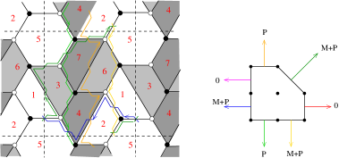
Figure 22: The rank distribution corresponding to $b_{1}=b_{5}=P$, $b_{2}=b_{4}=b_{7}=M+P$, $b_{3}=b_{6}=0$. The gauge groups are $SU(N)$ for faces 1, 2, 5; $SU(N+M)$ for faces 4, 7; $SU(N+M+P)$ for faces 6, 3.

Now the algorithm is the following: write every generating vector of $C^{*}$, with the exception of $(0,0,1)$, in the form $(c^{i},\eta_{0}(c^{i}))$, with $c^{i}$ given by the first two components and $\eta_{0}(c^{i})$ the third component. Find a point $a(c^{i})$ along the perimeter of the toric diagram satisfying $a(c^{i})\cdot c^{i}+\eta_{0}(c^{i})=0$. Then find a path representation for the point $a(c^{i})=\lambda^{i}_{j}d_{j}$ and compute for every $i$ the vector $\eta(c^{i})=(-\lambda^{i}_{1}(d_{1}\cdot c^{i}),\ldots,-\lambda^{i}_{7}(d_{7}\cdot c^{i}))$. We report the results in the following table:

$$\begin{array}[]{llclll}&c^{i}&\eta_{0}(c^{i})&a(c^{i})&\lambda^{i}&\eta(c^{i})\\ z_{1}&(0,1)&0&(0,0)&(0,0,0,0,0,0,0)&(0,0,0,0,0,0,0)\\ z_{2}&(-1,0)&2&(2,0)&(1,1,0,0,0,0,0)&(1,1,0,0,0,0,0)\\ z_{3}&(-1,-1)&3&(2,1)&(1,1,1,0,0,0,0)&(1,1,1,0,0,0,0)\\ z_{4}&(0,-1)&2&(1,2)&(1,1,1,1,0,0,0)&(0,0,1,1,0,0,0)\\ z_{5}&(1,0)&0&(0,2)&(1,1,1,1,1,0,0)&(-1,-1,0,1,1,0,0)\end{array}$$ (8.10)

Now every equation in (8.4) is replaced in the following way:

$$t^{a}\prod_{i}z_{i}^{p_{i}}=\prod_{i}z_{i}^{q_{i}}\quad\rightarrow\quad\prod_{i}t_{i}^{\left(\sum_{j}q_{j}\eta(c^{j})-p_{j}\eta(c^{j})\right)_{i}}z_{i}^{p_{i}}=\prod_{i}z_{i}^{q_{i}}$$ (8.11)

and one can show that the degree is conserved: $a=\sum_{i}\left(\sum_{j}q_{j}\eta(c^{j})-p_{j}\eta(c^{j})\right)_{i}$. Substituting the $t_{i}$ with the parametrization (8.9), we finally find the equations in the deformed case:

$$\begin{array}[]{lll}z_{1}z_{3}=z_{2}(t+S_{2})&z_{2}z_{4}=z_{3}t&z_{3}z_{5}=z_{4}(t+S_{1})\\ z_{2}z_{5}=t(t+S_{1})&z_{1}z_{4}=t(t+S_{2})&\end{array}$$ (8.12)

which still define a three dimensional complex geometry.

8.2 The moduli space of the gauge theory

First of all we have to compute the rank distribution in the gauge theory due to the fractional branes using our proposal in Section 5. As already said there are different ways to do that, exchanging the weights $b_{1}$ and $b_{2}$ or $b_{6}$ and $b_{7}$, but they all lead to a supersymmetric vacuum.

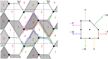
Figure 23: The rank distribution corresponding to $b_{3}=b_{6}=-P$, $b_{1}=b_{4}=b_{7}=-M$, $b_{2}=b_{5}=0$. The gauge groups are $SU(N)$ for faces 1, 4, 7, 5; $SU(N+M)$ for face 2; $SU(N+P)$ for face 6; $SU(N+P-M)$ for face 3.

In Figure 22 for example we report the choice: $(P,M+P,0,M+P,P,0,M+P)$ for the $b_{i}$. Using the charge distribution in Figure 19 it is easy to see that the ranks are: $(N,N,N+M+P,N+M,N,N+M+P,N+M)$. In the IR if $N=0$ we have a configuration equal to that of Figure 13, and hence we expect a supersymmetric vacuum.

In Figure 23 we draw the rank distribution for another possible choice of $b_{i}$: $(-M,0,-P,-M,0,-P,-M)$ which leads to the ranks: $(N,N+M,N+P-M,N,N$, $N+P,N)$. We will consider the case $P>M>0$. In the IR if $N=0$ there survive only the three isolated groups 2,3, and 6. Therefore this configuration is easier and we will study the moduli space in this case.

We have to consider a single $N=1$ regular brane. In the IR the non abelian gauge groups are 2,3 and 6 with ranks $SU(M+1)$, $SU(P-M+1)$ and $SU(P+1)$ and they all have $N_{f}<N_{c}$, developing ADS superpotential terms. We replace the chiral fields connected to these groups with the mesons $A,B,C$ of gauge groups $2,3,6$ respectively:

$$\begin{array}[]{l}A=\left(\begin{array}[]{ll}A_{14}&A_{15}\\ A_{74}&A_{75}\end{array}\right)\equiv\left(\begin{array}[]{ll}X_{12}X_{24}&X_{12}X_{25}\\ X_{72}X_{24}&X_{72}X_{25}\end{array}\right)\\[3.60004pt] B=\left(\begin{array}[]{ll}B_{14}&B_{15}\\ B_{74}&B_{75}\end{array}\right)\equiv\left(\begin{array}[]{ll}X_{13}X_{34}&X_{13}X_{35}\\ X_{73}X_{34}&X_{73}X_{35}\end{array}\right)\\[3.60004pt] C=\left(\begin{array}[]{ll}C_{41}&C_{47}\\ C_{51}&C_{57}\end{array}\right)\equiv\left(\begin{array}[]{ll}X_{46}X_{61}&X_{46}X_{67}\\ X_{56}X_{61}&X_{56}X_{67}\end{array}\right)\end{array}$$ (8.13)

and the superpotential is:

$$W = A_{75}C_{57}+B_{75}X_{57}+C_{41}A_{14}+B_{14}X_{45}X_{51}$$ (8.14)

$$-A_{74}X_{45}X_{57}-C_{51}B_{15}-B_{74}C_{47}-A_{15}X_{51}$$

$$+\alpha\log(\det A)+\beta\log(\det B)+\gamma\log(\det C)$$

where we have rewritten $W_{0}$ through mesons and have added the three ADS terms using the glueballs $\alpha$, $\beta$, $\gamma$ that will be matched to the two deformation parameters $S_{1}$ and $S_{2}$, similarly as in [33]. The mesons $Z_{i}$ and $T$ can be rewritten as:

$$\begin{array}[]{lll}Z_{1}=C_{47}A_{74}&Z_{2}=B_{75}C_{57}&Z_{3}=X_{45}C_{57}B_{74}\\ Z_{4}=X_{45}X_{57}B_{74}&Z_{5}=X_{57}A_{75}&T=A_{15}X_{51}\end{array}$$ (8.15)

where again we do not write traces because, using mesons $A,B,C$, all fields are abelian. We will check that the deformed equations (LABEL:def) are satisfied, focusing on generic points where all the mesons are different from zero. It is then easy to write the F-term equations from (8.14) and invert them to express some fields in function of the others. For example we found:

$$\begin{array}[]{lll}A_{14}=\displaystyle\frac{A_{74}(A_{74}X_{45}X_{57}-\alpha)}{A_{75}X_{51}}&A_{15}=\displaystyle\frac{A_{74}X_{45}X_{57}}{X_{51}}&B_{75}=\displaystyle A_{74}X_{45}\\[12.00003pt] B_{74}=\displaystyle\frac{A_{74}X_{45}X_{57}+\beta}{C_{47}}&B_{15}=\displaystyle\frac{A_{74}C_{47}}{X_{51}}&B_{14}=\displaystyle\frac{A_{74}X_{57}}{X_{51}}\\[12.00003pt] C_{51}=\displaystyle\frac{X_{51}(A_{74}X_{45}X_{57}+\beta)}{A_{74}C_{47}}&C_{57}=\displaystyle\frac{A_{74}X_{45}X_{57}-\alpha}{A_{75}}&C_{41}=\displaystyle\frac{A_{75}X_{51}}{A_{74}}\end{array}$$ (8.16)

and moreover F-term equations imply the relation:

$$\gamma=\alpha+\beta$$ (8.17)

so that indeed there are only two independent parameters.

Substituting into the explicit expressions for mesons (8.15) the results from F-term conditions (8.16) and (8.17), it is easy to prove that the mesons $Z_{i}$ satisfy relations analogous to (LABEL:def):

$$\begin{array}[]{lll}Z_{1}Z_{3}=Z_{2}(T+\beta)&Z_{2}Z_{4}=Z_{3}T&Z_{3}Z_{5}=Z_{4}(T-\alpha)\\ Z_{2}Z_{5}=T(T-\alpha)&Z_{1}Z_{4}=T(T+\beta)&\end{array}$$ (8.18)

so that the equations for the deformed geometry (LABEL:def) are correctly reproduced also in field theory, using the identifications:

$$\alpha=-S_{1}\qquad\beta=S_{2}$$ (8.19)

The same geometry has to be found using equivalent rank distributions, for instance that reported in Figure 22. We have studied the corresponding field theory in the simpler case $P=0$, that corresponds to a deformation with a single parameter $S_{1}=S_{2}$ (the toric diagram is split into the sum of a triangle and a square). With $N=1$, we have four non abelian $SU(M+1)$ gauge groups (faces $3,4,6,7$). By performing a Seiberg duality with respect to groups $7$ and $4$ we are left with only two non-abelian gauge groups and one can repeat easily the computation of the quantum modified moduli space. We have checked again that the deformed geometry is correctly reproduced.

9 Conclusions

In this paper we have provided a simple method to compute anomaly free rank distributions in quiver gauge theories corresponding to fractional deformation branes or to $\mathcal{N}=2$ fractional branes. More generally we have suggested that an efficient qualitative understanding of the IR behavior of the gauge theory with fractional branes can be obtained by looking at the weights $b_{i}$ associated with external legs in the (p,q) web.

Note however that according to our proposal, and as already noted in [25], deformation branes and $\mathcal{N}=2$ fractional branes correspond to very special weights distributions for the legs of the (p,q) web and moreover they can appear only when the toric diagram satisfies certain conditions. More general distributions should lead to what we have called supersymmetry breaking behavior: for toric quiver gauge theories there have been found only examples of runaway behavior [25, 26, 27, 28, 29], but it would be interesting to know whether this is a general feature of this class of fractional branes or whether one can find cases with a meta-stable vacuum.

When the toric singularity can be smoothed by a complex deformation, we have seen that the gauge theory has a supersymmetric confining vacuum when no regular branes remain in the IR. We verified in a concrete example that the moduli space probed by a regular brane, when we use our rule for finding rank distributions of deformation branes, reproduces the deformed geometry: deformation parameters correspond to gaugino condensates. We also pointed out that the $\Psi$-map is a useful tool in performing these computations and can explain in the general superconformal case why the moduli space of the gauge theory built with the Fast Inverse Algorithm matches with the toric geometry description. But a more general understanding of the deformed case is required.

Another important problem to be further investigated is the existence and the behavior of cascades for the various classes of fractional branes. Many examples are known in the literature [24, 23, 29]; at least for fractional deformation branes and SB branes there seems to exist a cascade of Seiberg dualities that, after passing through a certain number of possibly different phases of the gauge theory, sends the dimer back to itself but with a decreased number of regular branes. However a general study of cascades requires a better understanding of the (toric) phases of the quiver gauge theory.

Acknowledgments

I would like to thank in primis Alberto Zaffaroni, and Andrea Brini, Davide Forcella, Amihay Hanany for useful discussions and kind encouragement. This work is supported in part by INFN and MURST under contract 2005-024045-004 and by the European Community’s Human Potential Programme MRTN-CT-2004-005104.

References

- [1] S. Benvenuti, S. Franco, A. Hanany, D. Martelli and J. Sparks, “An infinite family of superconformal quiver gauge theories with Sasaki-Einstein duals,” JHEP 0506 (2005) 064 [arXiv:hep-th/0411264].
- [2] S. Benvenuti and M. Kruczenski, “From Sasaki-Einstein spaces to quivers via BPS geodesics: L(p,q,r),” JHEP 0604 (2006) 033 [arXiv:hep-th/0505206].
- [3] A. Butti, D. Forcella and A. Zaffaroni, “The dual superconformal theory for L(p,q,r) manifolds,” JHEP 0509 (2005) 018 [arXiv:hep-th/0505220].
- [4] S. Franco, A. Hanany, D. Martelli, J. Sparks, D. Vegh and B. Wecht, “Gauge theories from toric geometry and brane tilings,” JHEP 0601 (2006) 128 [arXiv:hep-th/0505211].
- [5] J. P. Gauntlett, D. Martelli, J. Sparks and D. Waldram, “Supersymmetric AdS(5) solutions of M-theory,” Class. Quant. Grav. 21, 4335 (2004) [arXiv:hep-th/0402153]; “Sasaki-Einstein metrics on S(2) x S(3),” Adv. Theor. Math. Phys. 8 (2004) 711 [arXiv:hep-th/0403002]; “A new infinite class of Sasaki-Einstein manifolds,” Adv. Theor. Math. Phys. 8 (2006) 987 [arXiv:hep-th/0403038].
- [6] M. Cvetic, H. Lu, D. N. Page and C. N. Pope, “New Einstein-Sasaki spaces in five and higher dimensions,” Phys. Rev. Lett. 95 (2005) 071101 [arXiv:hep-th/0504225]; “New Einstein-Sasaki and Einstein spaces from Kerr-de Sitter,” arXiv:hep-th/0505223.
- [7] D. Martelli and J. Sparks, “Toric Sasaki-Einstein metrics on S**2 x S**3,” Phys. Lett. B 621 (2005) 208 [arXiv:hep-th/0505027].
- [8] A. Hanany and K. D. Kennaway, “Dimer models and toric diagrams,” arXiv:hep-th/0503149; S. Franco, A. Hanany, K. D. Kennaway, D. Vegh and B. Wecht, “Brane dimers and quiver gauge theories,” JHEP 0601 (2006) 096 [arXiv:hep-th/0504110].
- [9] A. Hanany and D. Vegh, “Quivers, tilings, branes and rhombi,” arXiv:hep-th/0511063.
- [10] M. Bertolini, F. Bigazzi and A. L. Cotrone, “New checks and subtleties for AdS/CFT and a-maximization,” JHEP 0412, 024 (2004) [arXiv:hep-th/0411249].
- [11] A. Hanany, P. Kazakopoulos and B. Wecht, “A new infinite class of quiver gauge theories,” JHEP 0508 (2005) 054 [arXiv:hep-th/0503177].
- [12] S. Benvenuti and M. Kruczenski, “Semiclassical strings in Sasaki-Einstein manifolds and long operators in N = 1 gauge theories,” arXiv:hep-th/0505046.
- [13] K. Intriligator and B. Wecht, “The exact superconformal R-symmetry maximizes a,” Nucl. Phys. B 667, 183 (2003) [arXiv:hep-th/0304128].
- [14] D. Martelli, J. Sparks and S. T. Yau, “The Geometric Dual of a-maximization for Toric Sasaki-Einstein Manifolds,” arXiv:hep-th/0503183.
- [15] A. Butti and A. Zaffaroni, “R-charges from toric diagrams and the equivalence of a-maximization and Z-minimization,” JHEP 0511 (2005) 019 [arXiv:hep-th/0506232].
- [16] Y. Tachikawa, “Five-dimensional supergravity dual of a-maximization,” Nucl. Phys. B 733 (2006) 188 [arXiv:hep-th/0507057].
- [17] E. Barnes, E. Gorbatov, K. Intriligator and J. Wright, “Current correlators and AdS/CFT geometry,” Nucl. Phys. B 732 (2006) 89 [arXiv:hep-th/0507146].
- [18] S. Benvenuti, L. A. Pando Zayas and Y. Tachikawa, “Triangle anomalies from Einstein manifolds,” arXiv:hep-th/0601054.
- [19] S. Lee and S. J. Rey, “Comments on anomalies and charges of toric-quiver duals,” JHEP 0603 (2006) 068 [arXiv:hep-th/0601223].
- [20] C. P. Herzog and R. L. Karp, “Exceptional collections and D-branes probing toric singularities,” JHEP 0602 (2006) 061 [arXiv:hep-th/0507175].
- [21] A. Hanany, C. P. Herzog and D. Vegh, “Brane tilings and exceptional collections,” JHEP 0607 (2006) 001 [arXiv:hep-th/0602041].
- [22] I. R. Klebanov and M. J. Strassler, “Supergravity and a confining gauge theory: Duality cascades and chiSB-resolution of naked singularities,” JHEP 0008 (2000) 052 [arXiv:hep-th/0007191].
- [23] C. P. Herzog, Q. J. Ejaz and I. R. Klebanov, “Cascading RG flows from new Sasaki-Einstein manifolds,” JHEP 0502 (2005) 009 [arXiv:hep-th/0412193].
- [24] S. Franco, A. Hanany and A. M. Uranga, “Multi-flux warped throats and cascading gauge theories,” JHEP 0509 (2005) 028 [arXiv:hep-th/0502113].
- [25] S. Franco, A. Hanany, F. Saad and A. M. Uranga, “Fractional branes and dynamical supersymmetry breaking,” JHEP 0601 (2006) 011 [arXiv:hep-th/0505040].
- [26] D. Berenstein, C. P. Herzog, P. Ouyang and S. Pinansky, “Supersymmetry breaking from a Calabi-Yau singularity,” JHEP 0509 (2005) 084 [arXiv:hep-th/0505029].
- [27] M. Bertolini, F. Bigazzi and A. L. Cotrone, “Supersymmetry breaking at the end of a cascade of Seiberg dualities,” Phys. Rev. D 72 (2005) 061902 [arXiv:hep-th/0505055].
- [28] K. Intriligator and N. Seiberg, “The runaway quiver,” JHEP 0602 (2006) 031 [arXiv:hep-th/0512347].
- [29] A. Brini and D. Forcella, “Comments on the non-conformal gauge theories dual to Y(p,q) manifolds,” JHEP 0606 (2006) 050 [arXiv:hep-th/0603245].
- [30] S. Benvenuti, A. Hanany and P. Kazakopoulos, “The toric phases of the Y(p,q) quivers,” JHEP 0507 (2005) 021 [arXiv:hep-th/0412279].
- [31] K. Altmann, “The versal Deformation of an isolated toric Gorenstein Singularity,” arXiv:alg-geom/9403004.
- [32] I. Garcia-Etxebarria, F. Saad and A. M. Uranga, “Quiver gauge theories at resolved and deformed singularities using dimers,” JHEP 0606 (2006) 055 [arXiv:hep-th/0603108].
- [33] S. Pinansky, “Quantum deformations from toric geometry,” JHEP 0603 (2006) 055 [arXiv:hep-th/0511027].
- [34] A. Butti and A. Zaffaroni, “From toric geometry to quiver gauge theory: The equivalence of a-maximization and Z-minimization,” Fortsch. Phys. 54 (2006) 309 [arXiv:hep-th/0512240].
- [35] I. R. Klebanov and E. Witten, “Superconformal field theory on threebranes at a Calabi-Yau singularity,” Nucl. Phys. B 536, 199 (1998) [arXiv:hep-th/9807080].
- [36] B. S. Acharya, J. M. Figueroa-O’Farrill, C. M. Hull and B. Spence, “Branes at conical singularities and holography,” Adv. Theor. Math. Phys. 2, 1249 (1999) [arXiv:hep-th/9808014]; D. R. Morrison and M. R. Plesser, “Non-spherical horizons. I,” Adv. Theor. Math. Phys. 3, 1 (1999) [arXiv:hep-th/9810201].
- [37] Fulton, “Introduction to Toric Varieties”, Princeton University Press, Princeton 1993.
- [38] D. Martelli and J. Sparks, “Toric geometry, Sasaki-Einstein manifolds and a new infinite class of AdS/CFT duals,” Commun. Math. Phys. 262 (2006) 51 [arXiv:hep-th/0411238].
- [39] B. Feng, Y. H. He, K. D. Kennaway and C. Vafa, “Dimer models from mirror symmetry and quivering amoebae,” arXiv:hep-th/0511287.
- [40] A. Hanany and A. Iqbal, “Quiver theories from D6-branes via mirror symmetry,” JHEP 0204 (2002) 009 [arXiv:hep-th/0108137].
- [41] S. Benvenuti, A. Hanany, D. Martelli and J. Sparks, Work in progress.
- [42] S. Franco and D. Vegh, “Moduli spaces of gauge theories from dimer models: Proof of the correspondence,” arXiv:hep-th/0601063.