UNSTABLE STATES FOR CLOSED STRING
WITH MASSIVE POINT

Abstract

The stability problem for the hypocycloidal rotational states of the closed relativistic string with a point-like mass is solved with the help of analysis of small disturbances of these states. Both analytical and numerical investigations showed an unexpected result: the mentioned states turned out to be unstable. This conclusion is based upon the presence of roots with positive imaginary parts (increments) in the spectrum of frequencies of small disturbances. But these increments were small enough, so this instability had not been detected in previous numerical experiments. For the linear rotational states (the particular case of hypocycloidal states) the stability was confirmed. These results are important for applications of this model in hadron spectroscopy.

1. Introduction

In the previous work [1] we investigated the stability problem for 3 classes of rotational states of the closed string with a point-like mass. The corresponding exact solutions of the dynamical equations for this string were obtained in Ref. [2]. The closed string carrying one massive point moves in the space ${\cal M}=R^{1,3}\times T^{D-4}$, where $R^{1,3}$ is Minkowski space, $T^{D-4}$ is torus resulting from the compactification procedure [3]. We denote $x^{0},\dots,x^{3}$ the coordinates in $R^{1,3}$ and the torus $T^{D-4}$ has cyclic coordinates $x^{k}$ ($k=4,5\dots$) with periods $\ell_{k}$, that is, points with coordinates $x^{k}$ and $x^{k}+N_{k}\ell_{k}$, $N_{k}\in Z$ are identified. The metric in ${\cal M}$ is flat one: $ds^{2}=\eta_{\mu\nu}dx^{\mu}dx^{\nu}$, the corresponding basis $e_{0},\;e_{1},\;e_{2},\,\dots\,e_{D-1}$ is orthonormal one.

For two (from 3) classes of the mentioned rotational states in Ref. [1] we used two approaches of solving the stability problem: 1) numerical simulation of motions, close to the rotational ones, and 2) analytical investigation of small disturbances spectra for these states. The both approaches gave the same results. But for the third class — hypocycloidal rotational states we used only numerical simulation because of very sophisticated calculations in the spectral analysis. But later, when the calculations had been fulfilled, the unexpected results were obtained. They are presented in this paper.

2. Dynamics

The dynamics of the closed string (with the world surfaces $X^{\mu}(\tau,\sigma)$, $\sigma_{1}\leq\sigma\leq\sigma_{2})$ carrying a point-like mass $m$ in the space ${\cal M}$ is described by the system of equations [2]

$$\frac{\partial^{2}X^{\mu}}{\partial\tau^{2}}-\frac{\partial^{2}X^{\mu}}{\partial\sigma^{2}}=0,$$ (1)

$$X^{\mu}(\tau^{*},2\pi)=X^{\mu}(\tau,0)+\sum\limits_{k\geq 4}N_{k}\ell_{k}e^{\mu}_{k}$$ (2)

$$m\frac{d}{d\tau}\frac{\dot{X}^{\mu}(\tau,0)}{\sqrt{\dot{X}^{2}(\tau,0)}}+\gamma\big{[}X^{{}^{\prime}\!\mu}(\tau^{*},2\pi)-X^{{}^{\prime}\!\mu}(\tau,0)\big{]}=0,$$ (3)

which (without loss of generality) take this form under the conditions $\sigma_{1}=0$, $\sigma_{2}=2\pi$ and the orthonormality conditions on the world surface

$$(\partial_{\tau}X\pm\partial_{\sigma}X)^{2}=0.$$ (4)

Here $\gamma$ is the string tension, $\dot{X}^{\mu}\equiv\partial_{\tau}X^{\mu}$, $X^{{}^{\prime}\!\mu}\equiv\partial_{\sigma}X^{\mu}$; the scalar product is $(a,b)=\eta_{\mu\nu}a^{\mu}b^{\nu}$.

Equation (2) is the closure condition on the tube-like world surface of the closed sting on the world line of the massive point [4]. This line can be parameterized with two different parameters $\tau$ and $\tau^{*}$, connected by the relation $\tau^{*}=\tau^{*}(\tau).$ This relation should be added to the closure condition (2).

In this paper we consider the hypocycloidal rotational states corresponding to the following solutions of the system (1) – (4) [1], [2]:

$$\begin{array}[]{c}\displaystyle X^{\mu}(\tau,\sigma)=e_{0}^{\mu}a_{0}(\tau-\theta\sigma)+\sum\limits_{k>3}e^{\mu}_{k}b_{k}\sigma+\\ +A\Big{\{}\big{[}S\cos\omega\sigma+(C_{\theta}-C)\sin\omega\sigma\big{]}\cdot e^{\mu}(\omega\tau)-S_{\theta}\sin\omega\sigma\cdot\acute{e}^{\mu}(\omega\tau)\Big{\}}.\rule[8.53581pt]{0.0pt}{2.84526pt}\end{array}$$ (5)

Here $\displaystyle b_{k}=\frac{\ell_{k}N_{k}}{2\pi}$, $e^{\mu}(\omega\tau)=e^{\mu}_{1}\cos\omega\tau+e^{\mu}_{2}\sin\omega\tau$,

$\acute{e}^{\mu}(\omega\tau)=\omega^{-1}\frac{d}{d\tau}e^{\mu}(\omega\tau)$ are unit orthogonal rotating vectors, the speed of light $c=1$, the following values

$$Q=\frac{\gamma}{m}\sqrt{\dot{X}^{2}(\tau,0)}={}\mbox{const},\qquad\theta=\frac{\tau^{*}(\tau)-\tau}{2\pi}={}\mbox{const},$$ (6)

are constant for sulutions (5),

$$C=\cos 2\pi\omega,\;\quad S=\sin 2\pi\omega,\;\quad C_{\theta}=\cos 2\pi\theta\omega,\;\quad S_{\theta}=\sin 2\pi\theta\omega.$$ (7)

Values $a_{0}$, $A$ and speed of the massive point $v={}$const are connected by the equations

$$a_{0}=\frac{mQ}{\gamma\sqrt{1-v^{2}}},\qquad A=\frac{a_{0}v}{\omega S},\qquad v^{2}=\theta\frac{S}{S_{\theta}},$$ (8)

and values $\omega$ and $\theta$ are determined from the system [2]

$$C-C_{\theta}=\frac{\omega}{2Q}S,$$ (9)

$$(1+\theta^{2})\,SS_{\theta}-2\theta(1-CC_{\theta})=(S_{\theta}-\theta S)\frac{\beta S}{Q^{2}},$$ (10)

resulting from Eqs. (1) – (4). Here $\beta=(\gamma/m)^{2}\sum\limits_{k>3}b_{k}^{2}$

Solution of the system (9), (10) (pairs $\omega$, $\theta$) form some countable set. Each pair corresponds to solution (5) describing uniform rotation of the closed string with certain topological type. In the case $\beta=0$ the string has the form of a closed hypocycloid joined at non-zero angle in the massive point, so we use the term “hypocycloidal rotational states” for motions (5). These states generate non-trivial spectrum of Regge trajectories [2] and may be applied in the hadron spectroscopy.

Structure of solutions of the system (9), (10) is illustrated in Fig. 1. Here solid lines are determined by Eq. (9) and dashed lines form the graphical chart of Eq. (10) in the ($\omega,\theta$) plane. Here $Q=1$, $\beta=0.1$. Solutions ($\omega,\theta$) of this system are connected to cross points of these lines.

Note that solutions $\omega=n/2$, $\theta=(n-2k)/n$ of Eqs. (9), (10) correspond to hypocycloidal states (5) of the closed string with zero mass $m=0$. But other solutions (cross points in Fig. 1) result in states with $m\neq 0$. Projection of the string onto $e_{1},\,e_{2}$ plane is a curvilinear $n$-gon (a hypocycloid in the case $\beta=0$), where $n$ is the number of solid line in Fig. 1.

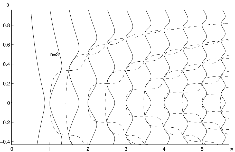
Figure 1: Graphical chart of Eq. (9) (solid lines) and Eq. (10) (dashed lines) for $Q=1$, $\beta=0.1$

In the particular case $\theta=0$ solutions (5) with frequencies $\omega$ (roots of Eq. (9), precisely, of equation $\omega=-2Q\tan\pi\omega$) have the form

$$X^{\mu}=e_{0}^{\mu}a_{0}\tau+\sum_{k>3}e^{\mu}_{k}b_{k}\sigma+A\cos\big{[}\omega(\sigma-\pi)\big{]}\cdot e^{\mu}(\omega\tau).$$ (11)

They describe uniform rotations of the sinusoidal string with rotating (along a circle) massive point. We name these motions as “linear rotational states”, because projections of the string onto $e_{1},\,e_{2}$ plane are rectilinear segments.

The third class of rotational states (with massive point at the center of rotation) was studied in detail in Ref. [1].

Possible applications of solutions (5) and (11) in hadron spectroscopy essentially depend on stability or instability of these states with respect to small disturbances. In the following section we study spectrum of these disturbances.

3. Spectrum of disturbances

To solve the stability problem for rotational motions (5), (11) we consider the general solution of Eq. (1)

$$X^{\mu}(\tau,\sigma)=\frac{1}{2}[\Psi^{\mu}_{+}(\tau+\sigma)+\Psi^{\mu}_{-}(\tau-\sigma)]$$ (12)

and denote

$$\breve{\Psi}^{\prime\mu}_{\pm}(\tau)=e_{0}^{\mu}(1\mp\theta)\,a_{0}\pm\sum_{k>3}e^{\mu}_{k}b_{k}+\omega A\Big{[}\pm(C_{\theta}-C)\,e^{\mu}(\omega\tau)+(S_{\theta}\mp S)\,\acute{e}^{\mu}(\omega\tau)\Big{]}$$ (13)

the functions in the expression (12) for the considered rotational motions (5).

To describe any small disturbances of the rotational motion of the system, that is motions close to states (5) we consider vector functions $\Psi^{\prime\mu}_{\pm}$ close to $\breve{\Psi}^{\prime\mu}_{\pm}$ in the form

$$\Psi^{\prime\mu}_{\pm}(\tau)=\breve{\Psi}^{\prime\mu}_{\pm}(\tau)+\varphi_{\pm}^{\mu}(\tau).$$ (14)

The disturbance $\varphi_{\pm}^{\mu}(\tau)$ is supposed to be small, so we omit squares of $\varphi_{\pm}$ when we substitute the expression (14) into dynamical equations (2) and (3). In other words, we work in the first linear vicinity of the states (5). Both functions $\Psi^{\prime\mu}_{\pm}$ and $\breve{\Psi}^{\prime\mu}_{\pm}$ in expression (14) must satisfy the condition ${\Psi^{\prime}_{+}\!\!}^{2}={\Psi^{\prime}_{-}\!\!}^{2}=0$, resulting from Eq.  (4), hence in the first order approximation on $\varphi_{\pm}$ the following scalar product equals zero:

$$\big{\langle}\breve{\Psi}^{\prime}_{\pm},\varphi_{\pm}\big{\rangle}=0.$$ (15)

For the disturbed motions the equality (6) $\tau^{*}=\tau+2\pi\theta$, generally speaking, is not carried out and should be replaced with the equality

$$\tau^{*}=\tau+2\pi\theta+\zeta(\tau),$$ (16)

where $\zeta(\tau)$ is a small disturbance.

Expression (14) together with Eq. (12) is the solution of the equations of string motion (1). Therefore we can obtain the equations of evolution of small disturbances $\varphi_{\pm}^{\mu}(\tau)$, substituting expressions (14) and (16) with Eq. (13) in two other equations of motion (2) and (3). We take into account the nonlinear factor $\big{[}\dot{X}^{2}(\tau,0)\big{]}^{-1/2}$ and contributions from the disturbed argument $\tau^{*}$ (16):

$$\breve{\Psi}^{\prime\mu}_{\pm}(\tau^{*}\pm 2\pi)\simeq\breve{\Psi}^{\prime\mu}_{\pm}(\pm)+\breve{\Psi}^{\prime\prime\mu}_{\pm}(\pm)\,\zeta(\tau).$$

Here and below $(\pm)\equiv(\tau+\tau_{0}\pm 2\pi)$.

This substitution results in the following linearized system of equations in linear (with respect to $\varphi_{\pm}^{\mu}$ and $\zeta$) approximation:

$$\begin{array}[]{c}\varphi_{+}^{\mu}(+)+\varphi_{-}^{\mu}(-)+2a_{0}\big{[}e_{0}^{\mu}+v\acute{e}^{\mu}(\omega\tau)\big{]}\,\zeta^{\prime}(\tau)-2a_{0}v\omega e^{\mu}(\omega\tau)\,\zeta(\tau)=\varphi_{+}^{\mu}(\tau)+\varphi_{-}^{\mu}(\tau),\\ \displaystyle\frac{d}{d\tau}\bigg{\{}\varphi_{+}^{\mu}(\tau)+\varphi_{-}^{\mu}(\tau)-\frac{1}{1-v^{2}}\big{[}e_{0}^{\mu}+v\acute{e}^{\mu}(\omega\tau)\big{]}\big{[}\varphi_{+}^{0}+\varphi_{-}^{0}+v(\acute{\varphi}_{+}+\acute{\varphi}_{-})\big{]}\bigg{\}}+\rule{0.0pt}{21.33955pt}\\ +Q\Big{[}\varphi_{+}^{\mu}(+)-\varphi_{-}^{\mu}(-)-\varphi_{+}^{\mu}(\tau)+\varphi_{-}^{\mu}(\tau)+2\omega^{2}A\big{[}(C-C_{\theta})\,\acute{e}^{\mu}+S_{\theta}e^{\mu}\big{]}\zeta(\tau)\Big{]}=0.\rule{0.0pt}{18.49428pt}\end{array}$$ (17)

Here we use the following notations for the scalar products:

$$\varphi_{\pm}^{0}\equiv\langle e_{0},\varphi_{\pm}\rangle,\quad\varphi_{\pm}^{k}\equiv\langle e_{k},\varphi_{\pm}\rangle,\quad\varphi_{\pm}\equiv\langle e,\varphi_{\pm}\rangle,\quad\acute{\varphi}_{\pm}\equiv\langle\acute{e},\varphi_{\pm}\rangle.$$ (18)

Projections (scalar products) of equations (17) onto vectors $e_{0}$, $e_{k}$, $e(\tau)$, $\acute{e}(\tau)$ form the following system of equations:

$$\begin{array}[]{c}\varphi_{+}^{k}(+)+\varphi_{-}^{k}(-)=\varphi_{+}^{k}(\tau)+\varphi_{-}^{k}(\tau),\\ \dot{\varphi}_{+}^{k}(\tau)+\dot{\varphi}_{-}^{k}(\tau)+Q\big{[}\varphi_{+}^{k}(+)-\varphi_{-}^{k}(-)-\varphi_{+}^{k}(\tau)+\varphi_{-}^{k}(\tau)\big{]}=0,\rule{0.0pt}{14.22636pt}\end{array}$$ (19)

$$\!\!\begin{array}[]{c}\varphi_{+}^{0}(+)+\varphi_{-}^{0}(-)-\varphi_{+}^{0}(\tau)-\varphi_{-}^{0}(\tau)+2a_{0}\dot{\zeta}(\tau)=0,\\ C_{+}\varphi_{+}(+)+C_{-}\varphi_{-}(-)-S_{+}\acute{\varphi}_{+}(+)-S_{-}\acute{\varphi}_{-}(-)-\varphi_{+}(\tau)-\varphi_{-}(\tau)+2a_{0}v\omega\zeta(\tau)=0,\rule{0.0pt}{14.22636pt}\\ C_{+}\acute{\varphi}_{+}(+)+C_{-}\acute{\varphi}_{-}(-)+S_{+}\varphi_{+}(+)+S_{-}\varphi_{-}(-)-\acute{\varphi}_{+}(\tau)-\acute{\varphi}_{-}(\tau)-2a_{0}v\dot{\zeta}(\tau)=0,\rule{0.0pt}{14.22636pt}\\ \frac{v}{1-v^{2}}\frac{d}{d\tau}\Big{[}v\varphi_{+}^{0}(\tau)+v\varphi_{-}^{0}(\tau)+\acute{\varphi}_{+}(\tau)+\acute{\varphi}_{-}(\tau)\Big{]}=Q\Big{[}f_{+}^{0}(+)-\varphi_{-}^{0}(-)-\varphi_{+}^{0}(\tau)+\varphi_{-}^{0}(\tau)\Big{]},\rule{0.0pt}{14.22636pt}\\ \dot{\varphi}_{+}+\dot{\varphi}_{-}-\frac{\omega}{1-v^{2}}\Big{[}v(\varphi_{+}^{0}+\varphi_{-}^{0})+\acute{\varphi}_{+}+\acute{\varphi}_{-}\Big{]}+\rule{0.0pt}{14.22636pt}\\ \!\!+Q\Big{[}C_{+}\varphi_{+}(+)-S_{+}\acute{\varphi}_{+}(+)-C_{-}\varphi_{-}(-)+S_{-}\acute{\varphi}_{-}(-)-\varphi_{+}(\tau)+\varphi_{-}(\tau)-2a_{0}\omega\frac{\theta}{v}\zeta(\tau)\Big{]}=0,\rule{0.0pt}{11.38109pt}\!\!\\ \omega(\varphi_{+}+\varphi_{-})+\frac{1}{1-v^{2}}\frac{d}{d\tau}\Big{[}v(\varphi_{+}^{0}+\varphi_{-}^{0})+\acute{\varphi}_{+}+\acute{\varphi}_{-}\Big{]}+\rule{0.0pt}{14.22636pt}\\ \!\!+Q\Big{[}C_{+}\acute{\varphi}_{+}(+)+S_{+}\varphi_{+}(+)-C_{-}\acute{\varphi}_{-}(-)-S_{-}\varphi_{-}(-)-\acute{\varphi}_{+}(\tau)+\acute{\varphi}_{-}(\tau)-a_{0}\omega^{2}\frac{v}{Q}\zeta(\tau)\Big{]}=0.\rule{0.0pt}{11.38109pt}\!\!\end{array}\!\!\!\!$$ (20)

Here $C_{\pm}=\cos\big{[}2\pi\omega(\theta\pm 1)\big{]}=C_{\theta}C\mp S_{\theta}S$, $S_{\pm}=S_{\theta}C\pm C_{\theta}S$, two equations (19) are projections of Eqs. (17) onto vectors $e_{k}$, $k=3,\,4,\dots$

We should add to this system equations (15) after substituting expressions (13)

$$(1\mp\theta)\,\varphi_{\pm}^{0}\pm\frac{1}{a_{0}}\sum_{k>3}b_{k}\varphi_{\pm}^{k}+\frac{v}{S}\big{[}\pm(C_{\theta}-C)\,\varphi_{\pm}+(S\mp S_{\theta})\,\acute{\varphi}_{\pm}\big{]}=0$$ (21)

System (19) – (21) is the linear system of differential equations with respect to projections (18) $\varphi_{\pm}^{0}(\tau)$, $\varphi_{\pm}^{k}(\tau)$, $\varphi_{\pm}(\tau)$, $\acute{\varphi}_{\pm}(\tau)$, and the function $\zeta(\tau)$. This system has constant coefficients but it also has deviating arguments $(\pm)$ together with $(\tau)$.

We search solutions of this system in the form of harmonics

$$\varphi_{\pm}^{0}=B_{\pm}^{0}e^{-i\tilde{\omega}\tau},\quad\varphi_{\pm}^{k}=B_{\pm}^{k}e^{-i\tilde{\omega}\tau},\varphi_{\pm}=B_{\pm}e^{-i\tilde{\omega}\tau},\quad\acute{\varphi}_{\pm}=\acute{B}_{\pm}e^{-i\tilde{\omega}\tau},\quad 2a_{0}\zeta=\Delta e^{-i\tilde{\omega}\tau}.$$ (22)

This substitution results in the linear homogeneous system of algebraic equations with respect to the amplitudes of harmonics (22). Two equations of this system connected with Eqs. (19) are

$$B_{+}^{k}E_{+}^{1}+B_{-}^{k}E_{-}^{1}=0,\qquad B_{+}^{k}(QE_{+}^{1}-i\tilde{\omega})=B_{-}^{k}(QE_{-}^{1}+i\tilde{\omega}),$$ (23)

where $E_{\pm}^{1}=\exp\big{[}-i2\pi(\theta\pm 1)\,\tilde{\omega}\big{]}-1$. System (23) has non-trivial solutions if and only if $\tilde{\omega}$ is a root of the equation

$$\cos 2\pi\tilde{\omega}-\cos 2\pi\theta\tilde{\omega}=\frac{\tilde{\omega}}{2Q}\sin 2\pi\tilde{\omega},$$ (24)

It coincides with Eq. (9), if $\omega$ is substituted by $\tilde{\omega}$. The spectrum of transversal (with respect to the $e_{1},\,e_{2}$ plane) small fluctuations of the string for states (5) contains frequencies $\tilde{\omega}$ which are roots of Eq. (24). All these frequencies are real numbers, therefore amplitudes of such fluctuations do not grow with growth of time $t$.

Another picture takes place for disturbances concerning to the $e_{1},\,e_{2}$ plane. Assuming that frequencies $\tilde{\omega}$ of these fluctuations are not roots of Eq. (24), we find for these modes $B_{\pm}^{k}=0$ and for other amplitudes (22) equations (20) and (21) result in the following system (after transforming):

$$\begin{array}[]{c}\tilde{\omega}(\acute{B}_{+}+\acute{B}_{-})+(\tilde{\omega}v-igQE^{1}_{+})\,B_{+}^{0}+(\tilde{\omega}v+igQE^{1}_{-})\,B_{-}^{0}=0,\\ \displaystyle h_{+}E^{1}_{+}\acute{B}_{+}-h_{-}E^{1}_{-}\acute{B}_{+}=\Big{(}i\frac{\omega v}{\tilde{\omega}}E^{1}_{+}-h^{*}_{+}E_{+}^{c}\Big{)}B_{+}^{0}+\Big{(}i\frac{\omega v}{\tilde{\omega}}E^{1}_{-}+h^{*}_{-}E_{-}^{c}\Big{)}B_{-}^{0},\rule{0.0pt}{18.49428pt}\\ (E_{+}+1)\,\acute{B}_{+}+(E_{-}+1)\,\acute{B}_{-}=(vE^{1}_{+}+h^{*}_{+}S_{+}E_{+})\,B_{+}^{0}+(vE^{1}_{+}-h^{*}_{-}S_{-}E_{-})\,B_{-}^{0},\rule{0.0pt}{14.22636pt}\\ \big{[}\omega q-h_{+}(E^{1}_{+}-i\tilde{\omega}/Q)\big{]}\acute{B}_{+}+\big{[}\omega q-h_{-}(E^{1}_{-}+i\tilde{\omega}/Q)\big{]}\acute{B}_{-}=\rule{0.0pt}{14.22636pt}\\ \displaystyle=\Big{[}i\frac{\omega\theta}{\tilde{\omega}v}E^{1}_{+}-v\omega q+h^{*}_{+}\Big{(}E_{+}^{c}-i\frac{\tilde{\omega}}{Q}\Big{)}\Big{]}B_{+}^{0}+\Big{[}i\frac{\omega\theta}{\tilde{\omega}v}E^{1}_{-}-v\omega q+h^{*}_{-}\Big{(}E_{-}^{c}+i\frac{\tilde{\omega}}{Q}\Big{)}\Big{]}B_{-}^{0};\rule{0.0pt}{18.49428pt}\\ (i\tilde{\omega}q+E^{1}_{+}+2\theta/v^{2})\,\acute{B}_{+}+(i\tilde{\omega}q-E^{1}_{-}+2\theta/v^{2})\,\acute{B}_{-}=\rule{0.0pt}{14.22636pt}\\ =\big{[}E^{*}_{+}+h^{*}_{+}(S_{+}E_{+}+\omega/Q)\big{]}B_{+}^{0}+\big{[}E^{*}_{-}+h^{*}_{-}(S_{-}E_{-}-\omega/Q)\big{]}B_{-}^{0},\rule{0.0pt}{14.22636pt}\\ \tilde{\omega}\Delta=-i(E^{1}_{+}B_{+}^{0}+E^{1}_{-}B_{-}^{0}),\qquad B_{\pm}=\pm(h^{*}_{\pm}B_{\pm}^{0}+h_{\pm}\acute{B}_{\pm}).\rule{0.0pt}{14.22636pt}\end{array}$$ (25)

Here we use notations

$$E_{\pm}=\exp\big{[}-i2\pi(\theta\pm 1)\,\tilde{\omega}\big{]},\qquad E_{\pm}^{1}=E_{\pm}-1,\qquad E_{\pm}^{c}=C_{\pm}E_{\pm}-1,\qquad E^{*}_{\pm}=i\frac{\omega^{2}v}{2Q\tilde{\omega}}E^{1}_{\pm}-iv\tilde{\omega}q$$

$$g=\frac{1-v^{2}}{v},\qquad h_{\pm}=\frac{2Q}{\omega}\Big{(}1\mp\frac{\theta}{v^{2}}\Big{)}=\frac{S\mp S_{\theta}}{C-C_{\theta}},\qquad h^{*}_{\pm}=\frac{2Q}{\omega}\frac{1\mp\theta}{v},\qquad q=\frac{1}{Q(1-v^{2})},$$

equations (7) – (10) and relations

$$C_{\pm}\pm h_{\pm}S_{\pm}=-1,\qquad h_{\pm}(C_{\pm}-1)=\pm S_{\pm}.$$

Notice that the fifth equations of system (25) is linear combination of the first three ones with coefficients $iq$, $\omega/(2Q)$ and $\theta/v^{2}$. Hence, the condition of existence of non-trivial solutions for this system is vanishing the determinant connected with the first four equations. This condition results in the following equation:

$$\begin{array}[]{c}\displaystyle\bigg{(}D\frac{\tilde{C}-\tilde{C}_{\theta}}{\tilde{\omega}^{2}}-4gQ\frac{\tilde{S}}{\tilde{\omega}}+V\tilde{C}_{\theta}-g\tilde{C}\bigg{)}\bigg{(}\frac{\omega^{2}v}{2Q}\frac{\tilde{S}}{\tilde{\omega}}+V\tilde{C}_{\theta}+g\tilde{C}\bigg{)}+f(\tilde{\omega})+\\ \displaystyle+i\frac{\omega^{2}v}{2Q\tilde{\omega}}\bigg{[}V\tilde{S}\tilde{S}_{\theta}+V_{\theta}(\tilde{C}\tilde{C}_{\theta}-1)+2gQ(\tilde{C}-\tilde{C}_{\theta})\frac{S\tilde{S}_{\theta}-S_{\theta}\tilde{S}}{S\tilde{\omega}}\bigg{]}=0.\rule{0.0pt}{17.07164pt}\end{array}$$ (26)

Here the notations like (7) are used, but with $\tilde{\omega}$ instead of $\omega$: $\tilde{C}=\cos 2\pi\tilde{\omega}$, $\tilde{S}=\sin 2\pi\tilde{\omega}$, $\tilde{C}_{\theta}=\cos 2\pi\theta\tilde{\omega}$, $\tilde{S}_{\theta}=\sin 2\pi\theta\tilde{\omega}$; and also

$$D=\omega^{2}(gh_{+}h_{-}+v^{-1}),\quad V=\frac{1-CC_{\theta}}{v}\cdot\frac{C-v^{2}C_{\theta}}{C-C_{\theta}},\quad V_{\theta}=\frac{SS_{\theta}}{v}\cdot\frac{C-v^{2}C_{\theta}}{C-C_{\theta}};$$

$$f(\tilde{\omega})=\Big{(}V^{2}-V_{\theta}^{2}+\frac{g\omega^{2}v-4g^{2}Q^{2}-DV}{\tilde{\omega}^{2}}\Big{)}\tilde{S}_{\theta}^{2}+\Big{[}\frac{g\theta}{v^{2}}(\omega^{2}v+8gQ^{2})+DV_{\theta}\Big{]}\frac{\tilde{S}\tilde{S}_{\theta}}{\tilde{\omega}^{2}}+$$

$$+S_{\theta}\bigg{[}4gQ\Big{(}\frac{S}{v}-v\frac{1-CC_{\theta}}{S}\Big{)}-\omega(C-v^{2}C_{\theta})\bigg{]}\frac{\tilde{C}\tilde{S}_{\theta}}{\tilde{\omega}}-\Big{(}V_{\theta}\tilde{C}_{\theta}-\frac{2gQ\theta}{v^{2}\tilde{\omega}}\tilde{S}\Big{)}^{2}.$$

Equation (26) has the imaginary part. One can expect that complex (or imaginary) roots $\tilde{\omega}=\tilde{\omega}_{r}+i\xi$ of this equation exist.

But in the case $\theta=0$ that is for linear rotational states (11) the mentioned imaginary part vanishes. In this case equalities $S_{\theta}=\tilde{S}_{\theta}=V_{\theta}=0$ take place, hence, the function $f(\tilde{\omega})=0$ and equation (26) decomposes into product of the following two equations:

$$2Q\tilde{\omega}\Big{[}v^{2}-C+(1-v^{2})\cos 2\pi\tilde{\omega}\Big{]}+\omega^{2}v^{2}\sin 2\pi\tilde{\omega}=0,$$ (27)

$$\left(\frac{\omega^{2}}{v}+4gQ^{2}\right)(1-\cos 2\pi\tilde{\omega})+4gQ\tilde{\omega}\sin 2\pi\tilde{\omega}+\tilde{\omega}^{2}\left(\frac{C-v^{2}}{v}+g\cos 2\pi\tilde{\omega}\right)=0.$$ (28)

Their roots were analyzed in Ref. [1]. It was shown that all roots of Eq. (27) and

Eq. (28) are real numbers, if all values satisfy natural physical restrictions, for example, $v<1$, $m>0$. The typical picture of these roots in the plane $\tilde{\omega}_{r},\,\xi$ is presented in Fig. 1a for Eq. (27) and in Fig. 1b for Eq. (28). Roots are points of intersection of zero level lines for real part Re$F(\tilde{\omega}_{r}+i\xi)=0$ (solid lines) or imaginary part (dashed lines) of the corresponding equation with $\tilde{\omega}=\tilde{\omega}_{r}+i\xi$.

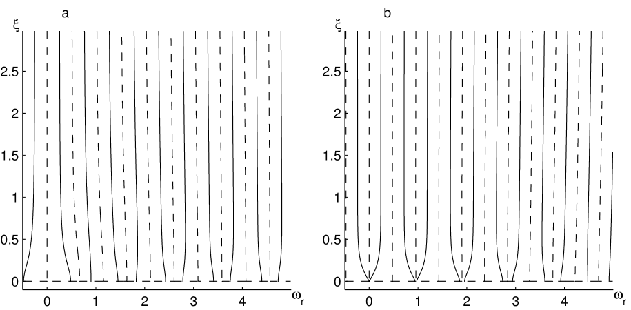
Figure 2: Zero level lines for real (solid) and imaginary part (dashed) for a) Eq. (27); b) Eq. (28)

Here the values of the parameters for the linear rotational state (11) are: $\omega=0.9$, $Q\simeq 1.385$, $v^{2}\simeq 0.875$, $\beta=0.5$. We may conclude that in first order approximation linear rotational states (11) are stable with respect to small disturbances.

Let us turn to the hypocycloidal rotational states (5) with spectral equation (26) for small disturbances.

Substituting $\tilde{\omega}=\tilde{\omega}_{r}+i\xi$ into Eq. (26) we draw in Figs. 3, 4 zero level lines for real part of l. h. s of this equation (solid lines) and for its imaginary part (dashed lines) similar to Fig. 2. In Fig. 3 these lines are shown for the hypocycloidal state (5) with the following values of parameters: $Q=1$, $\beta=0{.}1$, $\omega=1{.}289$, $\theta=0{.}3242$. The shape of the string (its projection onto $e_{1},\,e_{2}$ plane) at the corner of Fig. 3 is close to a curvilinear triangle.

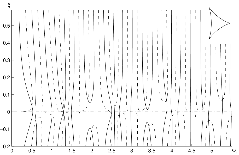
Figure 3: Zero level lines for real (solid) and imaginary part of Eq. (26) for the “triangle” state

In Fig. 4 the similar picture is drawn for the state (5) (hypocycloid with 4 arcs) for the recorded values of parameters.

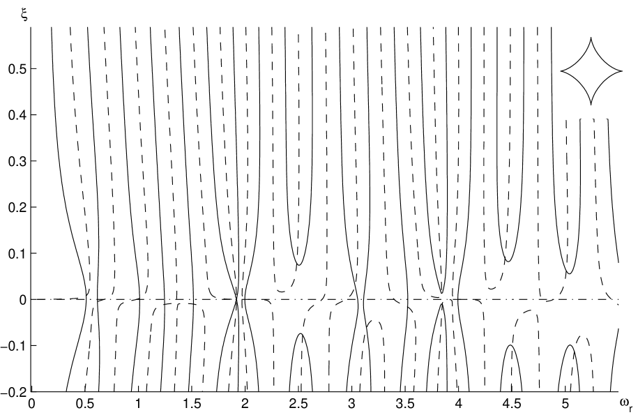
Figure 4: Zero level lines for real (solid) and imaginary part of Eq. (26), $Q=5$, $\beta=0$, $\omega=1{.}919$, $\theta=0{.}4996$

In both cases in Figs. 3, 4 one can find a set of cross points (roots of Eq. (26)) $\tilde{\omega}=\tilde{\omega}_{r}+i\xi$ with positive imaginary part $\xi>0$. The corresponding modes of disturbances $\varphi^{\mu}$ get the multiplier $\exp(\xi\tau)$, that is they grow exponentially. This picture takes place for any (physically admissible) values of parameters $Q$, $\beta$, $\omega$, $\theta$ so we may conclude that the hypocycloidal rotational states (5) for $\theta>0$ are unstable with respect to small disturbances.

But maximal increments $\xi$ for growing amplitudes are small: they do not exceed $0{.}1$ not only for the cases in Figs. 3, 4, but also for other topologically different hypocycloidal states with various values $Q$, $\beta$, $\omega$, $\theta$. So the growth factor for an amplitude of disturbance $\exp(2\pi\xi/\omega)$ (per one rotation) was not large enough to detect this instability in previous numerical experiments in Ref. [1]. On should add that the maximal increments $\xi$ tend to zero in both limits $Q\to 0$ (it corresponds to $m\to\infty$ if $a_{0}\gamma={}$const) and $Q\to\infty$ ($m\to 0$).

More detailed numerical simulation of string motions, close to hypocycloidal states (5) (slightly disturbed rotations) shows that amplitudes of small disturbances grow with increments $\xi$ described by Eq. (26).

Conclusion

The analysis of stability for the hypocycloidal rotational states (5) of the closed string with a point-like mass demonstrated instability of these states with $\theta\neq 0$ with respect to small disturbances. It is similar to behavior of rotational states of Y string baryon model [5], [6]. However, for the states (5) increments $\xi$ of this instability are small. For the linear rotational states (11) (the particular case of hypocycloidal states) the stability was confirmed.

This results are essential for possible applications of these states for describing excited hadrons with exotic properties (in particular, glueballs, hybrids, pentaquarks) in accordance with applications of other string hadron models [7] in meson and baryon spectroscopy.

References

• [1] A. E. Milovidov and G. S. Sharov, hep-th/0512330.
• [2] A. E. Milovidov, G. S. Sharov, Theor. Math. Phys. 142, 61 (2005); hep-th/0401070 .
• [3] M. B. Green, J. H. Schwarz, E. Witten, Superstring theory, Cambridge University Press, Cambridge, (1987) V. 1, 2.
• [4] G. S. Sharov, Phys. Rev. D58, 114009 (1998), hep-th/9808099.
• [5] G. S. Sharov, Phys. Rev. D62, 094015 (2000), hep-ph/0004003.
• [6] G.S. Sharov, Phys. Atom. Nucl. 65, 842 (2002).
• [7] G. S. Sharov, Phys. Atom. Nucl. 62, 1705 (1999).