From ${\cal N}=2$ supersymmetric classical
to quantum mechanics and back:
the SUSY WKB approximation

Abstract

Links between supersymmetric classical and quantum mechanics are explored. Diagrammatic representations for $\hbar$-expansions of norms of ground states are provided. The WKB spectra of supersymmetric non harmonic oscillators are found.

1 Introduction

In this essay, written to commemorate the sixtieth birthday of J. Cari$\tilde{\rm n}$ena, we discuss several elementary issues in one-dimensional supersymmetric quantum mechanics. The r$\hat{{\rm o}}$le of the Riccati equation in this framework has been thoroughly analyzed by Cari$\tilde{\rm n}$ena and collaborators at the highest level of mathematical rigor by approaching topics such as the factorization method or shape invariance from a group-theoretical point of view, see [2], [3] and [4]. Our purpose here is to approach these matters from a rather physical point of view. To construct a supersymmetric quantum mechanical system starting from a physical potential energy we shall be led to deal with the Hamilton-Jacobi or the Poisson equations, although in both cases there is an associated Riccati equation. We shall focus on studying the relationship between supersymmetric classical and quantum mechanical systems, following the standard References [5] and [6] and the more recent Lectures of A. Wipf [7]. In particular, models where supersymmetry is unbroken and instantons exist will be analyzed at length. The main motivation to discuss these 1D SUSY QM models is to take profit of the knowledge acquired to study highly non-trivial 2D systems as those proposed in [20]. Another issue to be treated with care is the semiclassical behavior of supersymmetric quantum systems, this done with the help of the enlightening paper of A. Comtet et al. [12].

2 R$\hat{{\rm o}}$le of the Hamilton-Jacobi, Riccati and Poisson
equations in SUSY quantum mechanics

Let us start with a natural Lagrangian of one degree of freedom and the action functional:

$$S=\int\,dt\left[\frac{m}{2}\frac{dx}{dt}\frac{dx}{dt}-V(x;\lambda,k)\right]\qquad,\qquad\qquad[\lambda]={\rm ML}^{-2}{\rm T}^{-2}\ ,\ [k]={\rm MT}^{-2}\qquad.$$ (1)

We shall consider potential energies $V(x;\lambda,k)$ that depend on two parameters $\lambda$ and $k$ of dimensions given in (1) and we shall introduce the non-dimensional variables: $x\rightarrow\sqrt{\frac{k}{\lambda}}\cdot x$, $t\rightarrow\sqrt{\frac{m}{k}}\cdot t$, $V(x;\lambda,k)=\frac{k^{2}}{\lambda}\,V(x)$, such that the action and the Hamiltonian read (non-dimensional variables will be used in what follows):

$$S=\frac{k^{\frac{3}{2}}m^{\frac{1}{2}}}{\lambda}\cdot\int\,dt\left[\frac{1}{2}\frac{dx}{dt}\frac{dx}{dt}-V(x)\right]\ ,\qquad H(p,x)=\frac{k^{2}}{\lambda}\,\left({1\over 2}p^{2}+V(x)\right)\ ,\qquad\ p=\frac{\partial L}{\partial\dot{x}}=\frac{dx}{dt}\qquad.$$

2.1 One-dimensional ${\cal N}=2$ SUSY classical mechanics

A ${\cal N}=2$ supersymmetric extension of a classical mechanical system of one degree of freedom is constructed as follows:

1. We add two “fermionic” degrees of freedom to the “bosonic” degree of freedom with the real coordinate $x$. The fermionic coordinates form a Grassman Majorana spinor:

$$\theta=\left(\begin{array}[]{c}\theta_{1}\\ \theta_{2}\end{array}\right)\hskip 42.67912pt,\hskip 42.67912pt\theta_{\alpha}\theta_{\beta}+\theta_{\beta}\theta_{\alpha}=0\qquad,\qquad\forall\,\alpha,\beta=1,2\,\,\,\qquad.$$

2. A superPoisson structure is defined in the phase superspace with coordinates $p,x,\theta_{1},\theta_{2}$ . Given two superfunctions $F$ and $G$ on the superspace, the Poisson superbracket

$$\{F,G\}_{P}=\frac{\partial F}{\partial p}\frac{\partial G}{\partial x}-\frac{\partial F}{\partial x}\frac{\partial G}{\partial p}+i\sum_{\alpha=1}^{2}\,F\frac{\stackrel{{\scriptstyle\leftarrow}}{{\partial}}}{\partial\theta_{\alpha}}\frac{\stackrel{{\scriptstyle\rightarrow}}{{\partial}}}{\partial\theta_{\alpha}}G$$

is read from the basic brackets: $\forall\,\alpha,\beta=1,2\,,\,$, $\{p,x\}_{P}=1$, $\{x,x\}_{P}=0$, $\{p,p\}_{P}=0$, $\{\theta_{\alpha},\theta_{\beta}\}_{P}=i\delta_{\alpha\beta}$.

Note that in the “soul” of the system - the subspace of the superspace spanned by the Grassman variables- the configuration space and the phase space coincide. The reason is that the Lagrangian ruling the dynamics of the fermionic variables is of first order in time derivatives. Thus, the time derivatives of Grassman variables will not appear in the Hamiltonian.

3. The classical SUSY charges: $Q_{1}=p\theta_{1}-\frac{dW}{dx}\theta_{2}$, $Q_{2}=p\theta_{2}+\frac{dW}{dx}\theta_{1}$, close the classical supersymmetric algebra:

$$\{Q_{1},Q_{1}\}_{P}=\{Q_{2},Q_{2}\}_{P}=2iH_{S}\qquad,\qquad\{Q_{\alpha},H_{S}\}_{P}=0\qquad,\qquad\{Q_{1},Q_{2}\}_{P}=0\qquad.$$

4. The classical Hamiltonian $H_{S}$

$$H_{S}=\frac{1}{2}p^{2}+\frac{1}{2}\frac{dW}{dx}\frac{dW}{dx}-i\frac{d^{2}W}{dx^{2}}\theta_{2}\theta_{1}\,\,$$ (2)

is invariant by construction with respect to the super-transformations generated by $Q_{1}$ and $Q_{2}$. Besides the kinetic energy of the bosonic variables, there are two interaction energy terms in the Hamiltonian (2) proportional to the (square of) the derivative and the second derivative of the arbitrary function $W(x)$, usually referred to as the superpotential.

Therefore, a given classical Hamiltonian:  $H={1\over 2}p^{2}+V(x)$, admits an extension to a ${\cal N}=2$ supersymmetric partner $H_{S}$ if and only if the superpotential satisfies

$${1\over 2}\frac{dW}{dx}\cdot\frac{dW}{dx}=V(x)$$ (3)

Note that $\frac{d^{2}W}{dx^{2}}$ enters in $H_{S}$ as the expectation value in Grassman states and disappears in a purely bosonic setting.

Let us now consider the Hamiltonian for the “flipped” potential $V(x)=-U(x)$ and the associated Hamilton-Jacobi equation:

$$H_{F}={1\over 2}p^{2}+U(x)\quad;\qquad\frac{\partial S}{\partial t}+H_{F}(\frac{\partial S}{\partial x},x)=0\qquad.$$

The time-independence of the Hamiltonian suggests solutions of the form $S(x,t)=-Et+W(x)$, leading to the reduced HJ equation:

$${1\over 2}\frac{dW}{dx}\cdot\frac{dW}{dx}+U(x)=E\qquad.$$ (4)

Therefore, the superpotential is no more than the Hamilton characteristic function for $E=0$ of the mechanical system with flipped potential. In sum, to find the superpotential, allowing for the supersymmetric extension of a classical mechanical system, one must solve a related Hamilton-Jacobi equation, see Reference [8].

In general, for any $E$, the Hamilton characteristic function is:

$$W(x;E)=\pm\int\,dx\sqrt{2(E-U(x))}\qquad\qquad.$$ (5)

The energy $E$ trajectories satisfy the ODE

$$\frac{dx}{dt}=\pm\frac{dW}{dx}=\pm\sqrt{2(E-U(x))}\quad\Rightarrow\quad\pm\int\,\frac{dx}{\sqrt{2(E-U(x))}}=t+t_{0}$$ (6)

2.2 One-dimensional ${\cal N}=2$ SUSY quantum mechanics

Canonical quantization of the above system to obtain the analogous ${\cal N}=2$ quantum supersymmetric system proceeds as follows, see, e.g., References [9], [10], [15] and [16]:

1. Replace Poisson brackets by commutators for the bosonic variables and anticommutators for the fermionic variables:

$$[\hat{x},\hat{p}]=\hat{x}\hat{p}-\hat{p}\hat{x}=i\bar{\hbar}\qquad,\qquad\{\hat{\theta}_{\alpha},\hat{\theta}_{\beta}\}=\hat{\theta}_{\alpha}\hat{\theta}_{\beta}+\hat{\theta}_{\beta}\hat{\theta}_{\alpha}=-\bar{\hbar}\delta_{\alpha\beta}\qquad,$$

where the non-dimensional Planck constant ${\bar{\hbar}}=\frac{\lambda\hbar}{m^{1\over 2}k^{3\over 2}}$ has been introduced.

2. We choose the coordinate representation for the bosonic variables but the classical Grassman variables become Fermi operators in the quantum domain: $\hat{p}={{\bar{\hbar}}\over i}{d\over dx}$, $\hat{x}=x$, $\hat{\theta}_{1}=\sqrt{{\bar{\hbar}}}\psi_{1}$, $\hat{\theta}_{2}=\sqrt{{\bar{\hbar}}}\psi_{2}$, $\{\psi_{1},\psi_{2}\}=0$.

The Fermi operators are represented on the Euclidean spinors in ${\mathbb{R}}^{2}$ by the anti-Hermitian $2\times 2$ Pauli matrices:

$$\psi_{1}=\frac{i}{\sqrt{2}}\sigma_{1}\ ,\quad\psi_{2}=-\frac{i}{\sqrt{2}}\sigma_{2}\ ,\quad\hat{\theta}_{1}^{2}=\hat{\theta}^{2}_{2}=-\frac{\bar{\hbar}}{2}\left(\begin{array}[]{cc}1&0\\ 0&1\end{array}\right)\ ,\quad\{\hat{\theta}_{1},\hat{\theta}_{2}\}=0\ ,\quad[\hat{\theta}_{1},\hat{\theta}_{2}]=i\bar{\hbar}\sigma_{3}\quad.$$

3. The quantum supercharges, $\hat{Q}_{1}=-\hat{\theta}_{1}\bar{\hbar}\frac{d}{dx}-i\hat{\theta}_{2}\frac{dW}{dx}$, $\hat{Q}_{2}=\hat{\theta}_{2}\bar{\hbar}\frac{d}{dx}+i\hat{\theta}_{1}\frac{dW}{dx}$, are

$$\hat{Q}_{1}=-i\sqrt{\frac{\bar{\hbar}}{2}}\left(\begin{array}[]{cc}0&\bar{\hbar}\frac{d}{dx}-\frac{dW}{dx}\\ \bar{\hbar}\frac{d}{dx}+\frac{dW}{dx}&0\end{array}\right)\ ,\qquad\hat{Q}_{2}=\sqrt{\frac{\bar{\hbar}}{2}}\left(\begin{array}[]{cc}0&-\bar{\hbar}\frac{d}{dx}+\frac{dW}{dx}\\ \bar{\hbar}\frac{d}{dx}+\frac{dW}{dx}&0\end{array}\right)$$

and satisfy the quantum algebra: $\{\hat{Q}_{1},\hat{Q}_{1}\}=\{\hat{Q}_{2},\hat{Q}_{2}\}=2\bar{\hbar}\hat{H}_{S}$, $\{\hat{Q}_{1},\hat{Q}_{2}\}=0$, $[\hat{Q}_{1},\hat{H}_{S}]=[\hat{Q}_{2},\hat{H}_{S}]=0$, with the quantum SUSY Hamiltonian:

$$\hat{H}_{S}=\left(\begin{array}[]{cc}\hat{h}^{(0)}&0\\ 0&\hat{h}^{(1)}\end{array}\right)={1\over 2}\left(\begin{array}[]{cc}-\bar{\hbar}^{2}\frac{d^{2}}{dx^{2}}+\frac{dW}{dx}\cdot\frac{dW}{dx}-\bar{\hbar}\frac{d^{2}W}{dx^{2}}&0\\ &\\ 0&-\bar{\hbar}^{2}\frac{d^{2}}{dx^{2}}+\frac{dW}{dx}\cdot\frac{dW}{dx}+\bar{\hbar}\frac{d^{2}W}{dx^{2}}\end{array}\right)\qquad.$$

It is also interesting to work with non-hermitian supercharges $\hat{Q}_{\pm}={1\over 2}(\hat{Q}_{1}\pm i\hat{Q}_{2})$,

$$\hat{Q}_{+}=-i\sqrt{\frac{\bar{\hbar}}{2}}\left(\begin{array}[]{cc}0&\bar{\hbar}\frac{d}{dx}-\frac{dW}{dx}\\ 0&0\end{array}\right)\ ,\ \hat{Q}_{-}=-i\sqrt{\frac{\bar{\hbar}}{2}}\left(\begin{array}[]{cc}0&0\\ \bar{\hbar}\frac{d}{dx}+\frac{dW}{dx}&0\end{array}\right)\qquad,$$

and reshuffle the quantum superalgebra in the form: $\{\hat{Q}_{+},\hat{Q}_{-}\}=2\bar{\hbar}\hat{H}_{S}$, $[\hat{Q}_{+},\hat{H}_{S}]=[\hat{Q}_{-},\hat{H}_{S}]=0$.

4. The quantum Hamiltonian is a block-diagonal $2\times 2$ matrix differential operator $\hat{h}^{(f=0)}$ and $\hat{h}^{(f=1)}$ are ordinary Schrödinger operators acting respectively on the subspaces of the Hilbert superspace labeled by the eigenvalues of the Fermi number operator:

$$\hat{f}=\hat{\theta}_{-}\cdot\hat{\theta}_{+}=\frac{\bar{\hbar}}{2}\cdot\left(\begin{array}[]{cc}0&0\\ 0&1\end{array}\right)\qquad,\qquad\hat{\theta}_{\pm}={i\over 2}(\hat{\theta}_{1}\pm i\hat{\theta}_{2})$$

5. Wave functions in the subspaces with zero and one Fermi number annihilated respectively by $\hat{Q}_{+}$ and $\hat{Q}_{-}$: $\hat{Q}_{+}\Psi_{0}^{(0)}(x)=0$, $\hat{Q}_{-}\Psi_{0}^{(1)}(x)=0$, are eigenfunctions of the Hamiltonian of zero energy. Therefore,

$$\Psi_{0}^{(0)}(x)=C{\footnotesize\left(\begin{array}[]{c}{\rm exp}[\bar{\hbar}^{-1}W(x)]\\ 0\end{array}\right)}\qquad,\qquad\Psi_{0}^{(1)}(x)=C{\footnotesize\left(\begin{array}[]{c}0\\ {\rm exp}[-\bar{\hbar}^{-1}W(x)]\end{array}\right)}$$

are the ground states of the supersymmetric quantum system if they are normalizable: $\int_{{\mathbb{R}}}\,dx\,e^{2W(x)\bar{\hbar}^{-1}}<+\infty$   ${\underline{\rm or}}$
$\int_{{\mathbb{R}}}\,dx\,e^{-2W(x)\bar{\hbar}^{-1}}<+\infty$. Note that either $\Psi_{0}^{(0)}$ or $\Psi_{0}^{(1)}$ can be normalizable.

2.3 The two-fold way to supersymmetric quantum mechanics

Given a physical system, the issue of building the associated supersymmetric quantum mechanics can be addressed in two different ways.

$\bullet$ Quantization of a classical supersymmetric system. In the first method, it is assumed that the classical supersymmetric extension has been performed. The identification of the classical superpotential requires that we must solve the ODE

$${1\over 2}{dW\over dx}{dW\over dx}=V(x)\qquad,$$

the time-independent Hamilton-Jacobi equation (4) for zero energy and flipped potential energy. This idea has been applied to integrable but not separable systems with two degrees of freedom in Reference [20]. Canonical quantization, as in the previous Section, provides all the interactions in the quantum system

$${\hat{V}}^{(0)}(x)={1\over 2}{dW\over dx}{dW\over dx}+{\bar{\hbar}\over 2}{d^{2}W\over dx^{2}}\qquad,\qquad{\hat{V}}^{(1)}(x)={1\over 2}{dW\over dx}{dW\over dx}-{\bar{\hbar}\over 2}{d^{2}W\over dx^{2}}$$

in terms of the Hamilton characteristic function.

$\bullet$ Supersymmetrization of a quantum system. The identification of the “quantum” superpotential would require one to solve one of the two Riccati differential equations

$${1\over 2}{d\hat{W}\over dx}{d\hat{W}\over dx}\pm{\bar{\hbar}\over 2}{d^{2}\hat{W}\over dx^{2}}=V(x)\qquad,$$ (7)

the sign marking the subspace where the the potential energy $V$ is expected to act. There is no dependence on the Planck constant in the potential energy of any physically significant mechanical system. Therefore, we change the strategy and look for superpotentials that solve the Poisson equation:

$$\pm{d^{2}\hat{W}_{P}\over dx^{2}}(x)=V(x)\qquad\qquad,$$ (8)

with the same criterion for the signs. Physically, this means that the Yukawa interactions provide the potential energy at stake. Mathematically, the solution of the Poisson equation (8) $\hat{W}_{P}$ provides a solution to a pair of related Riccati equations (9):

$${1\over 2}{d\hat{W}_{P}\over dx}{d\hat{W}_{P}\over dx}+{\bar{\hbar}\over 2}{d^{2}\hat{W}_{P}\over dx^{2}}=\hat{V}^{(0)}(x)\qquad,\qquad{1\over 2}{d\hat{W}_{P}\over dx}{d\hat{W}_{P}\over dx}-{\bar{\hbar}\over 2}{d^{2}\hat{W}_{P}\over dx^{2}}=\hat{V}^{(1)}(x)\qquad,$$ (9)

for other related potential energies: $\hat{V}^{(0)}(x)$, $\hat{V}^{(1)}(x)$. Once again, the datum is $V(x)$ in (8) from which $\hat{V}^{(0)}(x)$, $\hat{V}^{(1)}(x)$ are derived.

3 Examples: Anharmonic oscillators of sixth-order

To put these ideas to work, we choose as examples one-dimensional oscillators with terms proportional to $x^{4}$ and $x^{6}$ in the potential energy. Papers, reviews and even books dealing with the $x^{4}$ case abound. We shall discuss the $x^{6}$ case because it provides a splendid arena to disentangle two effects, instantons and spontaneous supersymmetry breaking, which in the $x^{4}$ case come together. The potential energies are:

$$V(x;\lambda,k)=\frac{\lambda^{2}}{2k}x^{2}\left(x^{2}\pm\frac{k}{\lambda}\right)^{2}\quad\qquad,\quad\qquad V(x)={1\over 2}\,x^{2}(x^{2}\pm 1)^{2}\quad,$$ (10)

describing respectively a single (+ sign) or triple (- sign) well. We shall only describe the first line of attack here from the solution to the HJ equation (where the potential energy is not found in the Yukawa interactions) and leave the Poisson route for another publication.

3.1 Quantization of classical supersymmetric sixth-order wells

3.1.1 Single well

1. Supersymmetric classical mechanics. The solution to the HJ equation for $E=0$ and $U(x)=-{1\over 2}x^{2}(x^{2}+1)^{2}$ is:

$$W(x)=\pm\int\,dx\,x(x^{2}+1)=\pm\left({x^{4}\over 4}+{x^{2}\over 2}\right)\qquad.$$

The supersymmetric classical Hamiltonian and the supercharges read:

$$H_{S}={1\over 2}p^{2}+{1\over 2}x^{2}(x^{2}+1)^{2}\mp i((3x^{2}+1)\theta_{2}\theta_{1}\qquad,\qquad Q_{\alpha}=p\theta_{\alpha}\mp x(x^{2}+1)\varepsilon_{\alpha\beta}\theta_{\beta}\qquad.$$

In the “soul” of the related supersymmetric system with flipped potential, the Hamilton characteristic function and the trajectories are given analytically by hyperelliptic integrals:

$$W(x;E)=\int\,dx\,\sqrt{x^{6}+2x^{4}+x^{2}+2E}\qquad,\qquad\int\,\frac{dx}{\sqrt{x^{6}+2x^{4}+x^{2}+2E}}=t+t_{0}\qquad.$$

For $E=0$, there is only one constant trajectory, where the particle sits on the top of the potential: $\bar{x}(t)=0$, which is also the unique BPS trajectory of the supersymmetric classical system.

2. Supersymmetric quantum mechanics. The quantum supercharges are:

$$\hat{Q}_{1}=-i\sqrt{\frac{\bar{\hbar}}{2}}\left(\begin{array}[]{cc}0&\bar{\hbar}\frac{d}{dx}\mp x(x^{2}+1)\\ \bar{\hbar}\frac{d}{dx}\pm x(x^{2}+1)&0\end{array}\right)\hskip 5.69046pt,\hskip 5.69046pt\hat{Q}_{2}=\sqrt{\frac{\bar{\hbar}}{2}}\left(\begin{array}[]{cc}0&-\bar{\hbar}\frac{d}{dx}\pm x(x^{2}+1)\\ \bar{\hbar}\frac{d}{dx}\pm x(x^{2}+1)&0\end{array}\right)\hskip 5.69046pt,$$ (11)

and the potential energies arising in $H_{S}$ read:

$$\hat{V}^{(0)}(x)={1\over 2}(x^{2}(x^{2}+1)^{2}\pm\bar{\hbar}(3x^{2}+1))\qquad,\qquad\hat{V}^{(1)}(x)={1\over 2}(x^{2}(x^{2}+1)^{2}\mp\bar{\hbar}(3x^{2}+1))\qquad.$$ (12)

Thus, the zero energy ground states are:

$$\Psi_{0}^{(0)}(x)=C\left(\begin{array}[]{c}{\rm exp}\{\pm\frac{({x^{4}\over 4}+{x^{2}\over 2})}{\bar{\hbar}}\}\\ 0\end{array}\right)\qquad,\qquad\Psi_{0}^{(1)}(x)=C\left(\begin{array}[]{c}0\\ {\rm exp}\{\frac{\mp({x^{4}\over 4}+{x^{2}\over 2})}{\bar{\hbar}}\}\end{array}\right)\qquad.$$

The supersymmetric quantum system has always one ground (BPS) state and supersymmetry is unbroken: if we choose $W={x^{4}\over 4}+{x^{2}\over 2}$ as the superpotential, the ground state belongs to the Fermi subspace - $\Psi_{0}^{(0)}$ is not normalizable-, the choice of $W={x^{2}\over 2}+{x^{4}\over 4}$ forces a Bosonic ground state whereas $\Psi_{0}^{(1)}$ becomes non-normalizable.

One can guess the energy and the type of eigen-function of the next energetic states by looking at the “effective” potentials:

$$V_{+}(x)={1\over 2}(x^{2}(x^{2}+1)^{2}-\bar{\hbar}(3x^{2}+1))\qquad,\qquad V_{-}(x)={1\over 2}(x^{2}(x^{2}+1)^{2}+\bar{\hbar}(3x^{2}+1))\qquad,$$

either $\hat{V}^{(0)}$ or $\hat{V}^{(1)}$ depending on the choice of $W$. The critical points of $V_{\pm}(x)$ are: $x_{0}=0$, $x_{1}^{\pm}=\pm\sqrt{-\frac{2-\sqrt{1\pm 9\bar{\hbar}}}{3}}$, $x_{2}^{\pm}=\pm\sqrt{\frac{-2+\sqrt{1\pm 9\bar{\hbar}}}{3}}$,

$${d^{2}V_{\pm}\over dx^{2}}(x_{0})=1\mp 3\bar{\hbar}\quad,\quad{d^{2}V_{\pm}\over dx^{2}}(x_{1}^{\pm})=4(1\pm 3\bar{\hbar}+\sqrt{1\pm 9\bar{\hbar}})\quad,\quad{d^{2}V_{\pm}\over dx^{2}}(x_{2}^{\pm})=4(1\pm 3\bar{\hbar}-\sqrt{1\pm 9\bar{\hbar}})\qquad.$$

$x_{0}$ is a minimum of $V_{+}$ if $\bar{\hbar}<{1\over 3}$ and becomes a maximum otherwise. $x_{1}^{\pm}$ are always imaginary roots but $x_{2}^{\pm}$ are real and become minima of $V_{+}$ for $\bar{\hbar}>{1\over 3}$.

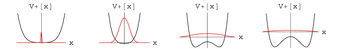
Figure 1: Potential energy ${\hat{V}}_{+}$ and BPS ground state $\Psi_{0}^{G}(x)$ (red) for:

(a) ${\bar{\hbar}}=0.001$, (b) ${\bar{\hbar}}=0.1$, (c) ${\bar{\hbar}}=2$, (d) ${\bar{\hbar}}=4$.

There is a unique minimum for $V_{-}$, $x_{0}$, and the wave function of the first level over the ground state is well approximated by a Gaussian around it:

$$\Psi_{-}^{E_{1}^{-}}(x)\simeq\left(\frac{\omega_{-}}{\bar{\hbar}\pi}\right)^{{1\over 4}}\left(\begin{array}[]{c}0\\ {\rm exp}\{-{\omega_{-}\over 2\bar{\hbar}}x^{2}\}\end{array}\right)\qquad,\qquad\omega_{-}=\sqrt{1+3\bar{\hbar}}\qquad,\qquad E_{-}^{E_{1}^{-}}\simeq{\bar{\hbar}\over 2}(1+\omega_{-})\qquad.$$ (13)

The supersymmetric partner state in the subspace of $\Psi_{0}^{G}$ is obtained by acting on $\Psi_{-}^{E_{1}^{-}}$ with $\hat{Q}_{+}$:

$$\Psi_{+}^{E_{1}^{+}}(x)=\hat{Q}_{+}\Psi_{-}^{F}(x)=\left(\frac{\omega_{-}\bar{\hbar}}{4\pi}\right)^{{1\over 4}}\left(\begin{array}[]{c}(x^{3}+(1+\omega_{-})x){\rm exp}[-{\omega_{-}\over\bar{\hbar}}x^{2}]\\ 0\end{array}\right)\ ,\ E_{1}^{+}=E_{1}^{-}\qquad.$$ (14)

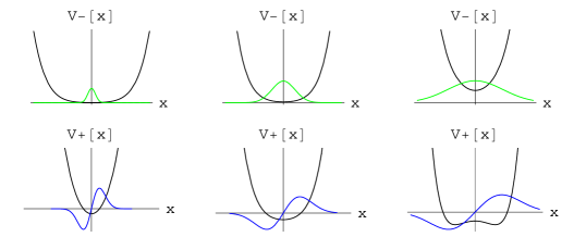
Figure 2: Potential energies ${\hat{V}}_{\pm}$. Degenerate in energy $\Psi_{-}^{E_{1}^{-}}(x)$ (green)

and $\Psi_{+}^{E_{1}^{+}}(x)$ (blue) wave functions: (a) ${\bar{\hbar}}=0.01$, (b) ${\bar{\hbar}}=0.1$, (c) ${\bar{\hbar}}=1$.

3. Zero-energy ground state. The dependence of $\Psi_{0}^{G}(x)={\rm exp}[-{({x^{4}\over 4}+{x^{2}\over 2})\over\bar{\hbar}}]$ on $\bar{\hbar}$ is rather involved and can be described analytically through the asymptotic behavior when $\bar{\hbar}\rightarrow\bar{\hbar}_{c}$ and $\bar{\hbar}_{c}=0$ is the classical value:

$${\rm exp}[-\frac{1}{2\bar{\hbar}}({x^{4}\over 2}+x^{2})]\simeq\lim_{\bar{\hbar}_{c}\rightarrow 0}{\rm exp}[-\frac{1}{\bar{\hbar}_{c}}({x^{4}\over 2}+x^{2})]\left\{1+{1\over\bar{\hbar}_{c}^{2}}\cdot\left(\frac{2\bar{\hbar}}{({x^{4}\over 2}+x^{2})}-\bar{\hbar}_{c}\right)\right.$$

$$+ \left.\frac{1-2\bar{\hbar}_{c}}{2\bar{\hbar}_{c}^{4}}\cdot\left(\frac{2\bar{\hbar}}{({x^{4}\over 2}+x^{2})}-\bar{\hbar}_{c}\right)^{2}+\frac{1+6\bar{\hbar}_{c}(\bar{\hbar}_{c}-1)}{6\bar{\hbar}_{c}^{6}}\cdot\left(\frac{2\bar{\hbar}}{({x^{4}\over 2}+x^{2})}-\bar{\hbar}_{c}\right)^{3}+\cdots\right\}\qquad.$$

It is also interesting to analyze how the norm of the BPS ground state $\Psi_{0}^{G}(x)$ depends on $\bar{\hbar}$:

$$N(\bar{\hbar})=\int\,dx\,{\rm exp}\left\{-\frac{x^{4}}{2\bar{\hbar}}-\frac{x^{2}}{\bar{\hbar}}\right\}=\sqrt{\bar{\hbar}}\int\,dz\,{\rm exp}\left\{-\frac{\bar{\hbar}z^{4}}{2}-z^{2}\right\}\qquad,\qquad x=\sqrt{\bar{\hbar}}z\qquad.$$ (15)

This non-gaussian integral is no more than the partition function ${\cal Z}(\bar{\hbar})=N(\bar{\hbar})$ of a QFT system in (0+0)-spacetime dimensions and Lagrangian [11]:

$$L=-{1\over 2}\varphi^{2}-{\lambda\over 4!}\varphi^{4}\qquad,\qquad z={\varphi\over\sqrt{2}}\quad,\quad\lambda=3\bar{\hbar}\qquad.$$ (16)

The partition function can be expressed as a series in $\bar{\hbar}$,

$${\cal Z}(\bar{\hbar})=\sum_{m=0}^{\infty}\int_{-\infty}^{\infty}\,dz\,{(-3\bar{\hbar})^{m}\over(4!)^{m}m!}\,z^{4m}\,e^{-z^{2}}\qquad,\qquad\int_{-\infty}^{\infty}\,dz\,z^{4m}\,e^{-z^{2}}=\frac{(4m)!}{(2m)!2^{2m}}\cdot\sqrt{\pi}\quad,$$ (17)

by performing infinite Gaussian integrals:

$${{\cal Z}(\bar{\hbar})\over\sqrt{\bar{\hbar}\pi}}=\sum_{m=0}^{\infty}{(-3\bar{\hbar})^{m}\over(4!)^{m}m!}\cdot{(4m)!\over(2m)!2^{2m}}=1-{1\over 8}(3\bar{\hbar})+{5\cdot 7\over 3\cdot 2^{7}}(3\bar{\hbar})^{2}-{5\cdot 7\cdot 11\over 3\cdot 2^{10}}(3\bar{\hbar})^{3}+\cdots\qquad.$$ (18)

The expansion (18) of the partition function shows an essential singularity at $\bar{\hbar}=0$ -the classical limit- and it is an asymptotic series. The best approximation to the integral is reached by keeping a number of terms $m_{0}$ such that the quotient between two consecutive terms is of the order of one:

$$\left|{a_{m_{0}+1}\over a_{m_{0}}}\right|={(4m_{0}+3)(4m_{0}+1)\over 4!(m_{0}+1)}|3\bar{\hbar}|\approx\bar{\hbar}2m_{0}\approx 1\Rightarrow m_{0}\approx{1\over 2\bar{\hbar}}\qquad,$$

and the error assumed by neglecting higher-order terms is bounded by ${\rm exp}[-{1\over 2\bar{\hbar}}]$.

It is tempting to explain the pictorial description of the series using Feynman diagram technology. Writing the partition function in the form,

$${{\cal Z}[\lambda]\over\sqrt{\lambda/3}}=\sum\int{\overbrace{{(-\lambda)\varphi^{4}\over 4!}\times\cdots\times{(-\lambda)\varphi^{4}\over 4!}}\over m!}e^{\left(-{1\over 2}\varphi^{2}\right)}d\varphi\quad,$$ (19)

one discovers the following Feynman rule: there is a single tetravalent vertex with a factor $(-\lambda)$. The lower-order terms in the series (18) correspond to the weights of the vacuum diagrams - the $-\lambda$ factor of the vertex divided by the combinatorial factor, the number of equivalent graphs of the same topological type- up to second order in perturbation theory shown in the next Table.

Vacuum graph		Weight	Vacuum graph		Weight
	$\rightarrow$	$1$
	$\rightarrow$	$-{\displaystyle{\lambda\over 2^{3}}}$		$\rightarrow$	${\displaystyle{\lambda^{2}\over 2^{4}}}$
	$\rightarrow$	${\displaystyle{\lambda^{2}\over 2^{7}}}$		$\rightarrow$	${\displaystyle{\lambda^{2}\over 3\cdot 2^{4}}}$

3.1.2 Triple well

1. Supersymmetric classical mechanics. The solution to the HJ equation for $E=0$ and $U(x)=-{1\over 2}x^{2}(x^{2}-1)^{2}$ is:

$$W(x)=\pm\int\,dx\,x(x^{2}-1)=\pm\left(\frac{x^{4}}{4}-\frac{x^{2}}{2}\right)\qquad.$$

The superpotential is thus the “sombrero” potential. The supersymmetric classical Hamiltonian and the supercharges read:

$$H_{S}={1\over 2}p^{2}+{1\over 2}x^{2}(x^{2}-1)^{2}\mp i((3x^{2}-1)\theta_{2}\theta_{1}\qquad,\qquad Q_{\alpha}=p\theta_{\alpha}\mp x(x^{2}-1)\varepsilon_{\alpha\beta}\theta_{\beta}\qquad.$$

Although feasible, we shall not attempt to search for trajectories with non-null Grassman degrees of freedom.

It is interesting, instead, to look at solutions in the “body” of the related supersymmetric system with flipped potential because of their r$\hat{\rm o}$le in the quantum $H_{S}$ system. The Hamilton characteristic function and the trajectories are given analytically by hyperelliptic integrals:

$$W(x;E)=\int\,dx\,\sqrt{x^{6}-2x^{4}+x^{2}+2E}\qquad,\qquad\int\,\frac{dx}{\sqrt{x^{6}-2x^{4}+x^{2}+2E}}=t+t_{0}\qquad.$$

For $E=0$, the integrations are easily performed and two kinds of trajectories are found:

$\bullet$ Constant trajectories, where the particle sits on the top of the potential:  $\bar{x}(t)=0$, $\bar{x}(t)=\pm 1$.

$\bullet$ Trajectories where the particle starts from a maximum of the potential at $t=-\infty$ and slowly moves to reach $x=\pm\infty$ (infinite action) or another maximum (finite action) at $t=\infty$.

$$x^{2}>1:\ \bar{x}^{2}(t)={1\over 1-e^{\pm 2(t+t_{0})}}\hskip 14.22636pt,\hskip 14.22636ptx^{2}<1,\,\,{\underline{\rm instanton}}:\ \bar{x}(t)=\pm\frac{1}{\sqrt{1+e^{\pm 2(t+t_{0})}}}\qquad.$$

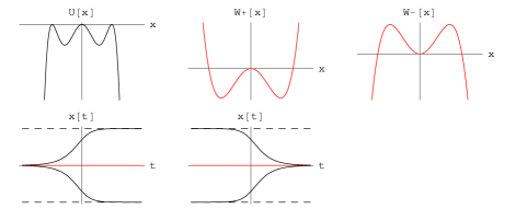
Figure 3: (a) Potential energy $U(x)$. (b) Hamilton characteristic function (superpotential) $W^{\pm}(x)$.

(c) Zero-energy, finite action, trajectories (instantons).

The constant trajectories are special due to the fact that they are also zero energy (BPS) classical solutions to $H_{S}$ because the classical supercharges $Q_{\pm}=(p\mp ix(x^{2}-1))\theta_{\pm}$ are annihilated by them for any value of $\theta_{\pm}$.

2. Supersymmetric quantum mechanics. The quantum supercharges are:

$$\hat{Q}_{1}=-i\sqrt{\frac{\bar{\hbar}}{2}}\left(\begin{array}[]{cc}0&\bar{\hbar}\frac{d}{dx}\mp x(x^{2}-1)\\ \bar{\hbar}\frac{d}{dx}\pm x(x^{2}-1)&0\end{array}\right)\hskip 5.69046pt,\hskip 5.69046pt\hat{Q}_{2}=\sqrt{\frac{\bar{\hbar}}{2}}\left(\begin{array}[]{cc}0&-\bar{\hbar}\frac{d}{dx}\pm x(x^{2}-1)\\ \bar{\hbar}\frac{d}{dx}\pm x(x^{2}-1)&0\end{array}\right)\hskip 5.69046pt,$$ (20)

and the potential energies arising in $H_{S}$ read:

$$\hat{V}^{(0)}(x)={1\over 2}(x^{2}(x^{2}-1)^{2}\pm\bar{\hbar}(3x^{2}-1))\qquad,\qquad\hat{V}^{(1)}(x)={1\over 2}(x^{2}(x^{2}-1)^{2}\mp\bar{\hbar}(3x^{2}-1))\qquad.$$ (21)

Thus, the zero-energy ground states are:

$$\Psi_{0}^{(0)}(x)=C\left(\begin{array}[]{c}{\rm exp}\{\pm\frac{({x^{4}\over 4}-{x^{2}\over 2})}{\bar{\hbar}}\}\\ 0\end{array}\right)\qquad,\qquad\Psi_{0}^{(1)}(x)=C\left(\begin{array}[]{c}0\\ {\rm exp}\{\frac{\mp({x^{4}\over 4}-{x^{2}\over 2})}{\bar{\hbar}}\}\end{array}\right)\qquad.$$

The supersymmetric quantum system always has one ground (BPS) state and supersymmetry is unbroken: if we choose $W={x^{4}\over 4}-{x^{2}\over 2}$ as superpotential the ground state belongs to the Fermi subspace - $\Psi_{0}^{(0)}$ is not normalizable-, the choice of $W={x^{2}\over 2}-{x^{4}\over 4}$ forces a bosonic ground state whereas $\Psi_{0}^{(1)}$ becomes non normalizable.

Nevertheless, despite unbroken supersymmetry this system has instantons. To analyze the coexistence of these two phenomena one needs to study how

$$V_{+}(x)={1\over 2}(x^{2}(x^{2}-1)^{2}-\bar{\hbar}(3x^{2}-1))\qquad,\qquad V_{-}(x)={1\over 2}(x^{2}(x^{2}-1)^{2}+\bar{\hbar}(3x^{2}-1))$$

evolve in response to changes in $\bar{\hbar}$. Note that either $V_{+}$ or $V_{-}$ are either $\hat{V}^{(0)}$ or $\hat{V}^{(1)}$, depending on the choice of $W$. The critical points of $V_{\pm}(x)$ are: $x_{0}=0$, $x_{1}^{\pm}=\pm\sqrt{\frac{2-\sqrt{1\pm 9\bar{\hbar}}}{3}}$, $x_{2}^{\pm}=\pm\sqrt{\frac{2+\sqrt{1\pm 9\bar{\hbar}}}{3}}$,

$${d^{2}V_{\pm}\over dx^{2}}(x_{0})=1\mp 3\bar{\hbar}\quad,\quad{d^{2}V_{\pm}\over dx^{2}}(x_{1}^{\pm})=4(1\pm 3\bar{\hbar}-\sqrt{1\pm 9\bar{\hbar}})\quad,\quad{d^{2}V_{\pm}\over dx^{2}}(x_{2}^{\pm})=4(1\pm 3\bar{\hbar}+\sqrt{1\pm 9\bar{\hbar}})\qquad.$$

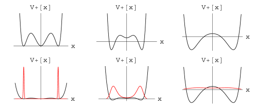
Figure 4: Potential energy $V_{+}$ and BPS wave function $\Psi_{0}^{G}(x)$ (red) plotted as functions of x

for several values of $\bar{\hbar}$: (a) ${\bar{\hbar}}=0.001$, (b) ${\bar{\hbar}}=0.1$, (c) ${\bar{\hbar}}=2$.

$x_{2}^{\pm}$ are always minima of $V_{+}(x)$, $x_{0}$ is a minimum of $V_{+}$ if $\bar{\hbar}<{1\over 3}$ but becomes a maximum if $\bar{\hbar}>{1\over 3}$, and $x_{1}^{\pm}$ are maxima of $V_{+}$ for $\bar{\hbar}<{1\over 3}$, not anymore critical point for $\bar{\hbar}>{1\over 3}$, see Figure 2. Therefore, because $V_{+}(x_{0})={\bar{\hbar}\over 2}>V_{+}(x_{2}^{\pm})=\frac{2+\sqrt{1+9\bar{\hbar}}}{3}\left[{1-\sqrt{1+9\bar{\hbar}}\over 9}-2\bar{\hbar}\right]+{\bar{\hbar}\over 2}$, $x_{0}$ is a false vacuum that decays to the true vacua $x_{2}^{\pm}$ when $\bar{\hbar}<{1\over 3}$. The decay amplitude can be computed from the classical bounce for the flipped potential, starting and ending at $x_{0}$, which is very well approximated by an instanton-anti-instanton configuration for small values of $\bar{\hbar}$. It is remarkable how well this behavior is described by the ground state wave function $\Psi^{G}_{0}(x)$; even more remarkable, $\Psi_{0}^{G}(x)$ also matches the expected behavior for $\bar{\hbar}>{1\over 3}$ where there is no tunnel effect at all, see again Figure 2.

$x_{0}$, however, is the absolute minimum of $V_{-}(x)$; if $\bar{\hbar}<{1\over 9}$, $x_{2}^{\pm}$ are also minima of $V_{-}(x)$, but $V_{-}(x_{0})=-{\bar{\hbar}\over 2}<V_{-}(x_{2}^{\pm})=\frac{2+\sqrt{1-9\bar{\hbar}}}{3}\left[{1-\sqrt{1-9\bar{\hbar}}\over 9}+2\bar{\hbar}\right]-{\bar{\hbar}\over 2}$. If $\bar{\hbar}>{1\over 9}$ $x_{0}$ is the single critical point (minimum) of $V_{-}(x)$. Therefore, the eigenfunction of the lowest eigenvalue of the Schrodinger operator with potential energy $V_{-}(x)$ is approximately a Gaussian centered at $x_{0}=0$:

$$\Psi_{-}^{E_{1}^{-}}(x)\simeq\left(\frac{\omega_{-}}{\bar{\hbar}\pi}\right)^{{1\over 4}}\cdot{\rm exp}\{-{\omega_{-}\over 2\bar{\hbar}}x^{2}\}\ ,\qquad\omega_{-}=\sqrt{1+3\bar{\hbar}}\qquad,\qquad E_{1}^{-}\simeq{\bar{\hbar}\over 2}(\omega_{-}-1)\qquad.$$ (22)

$\Psi_{-}^{E_{1}^{-}}(x)$, the first eigenfunction of $H_{s}$ outside the kernel, lives in the subspace orthogonal to the subspace of $\Psi^{G}(x)$. For $\bar{\hbar}<{1\over 9}$, $\Psi_{-}^{E_{1}^{-}}$ grows from the decay of the false vacua $x_{2}^{\pm}$ ruled by instantons/anti-instantons now starting and ending at $x_{2}^{\pm}$. Mathematica drawings of these wave functions are offered in Figure 3.

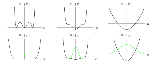
Figure 5: Potential energy $V_{-}(x)$ and wave function $\Psi_{-}^{E_{1}^{-}}(x)$ (green) plotted as functions of $x$

for several values of $\bar{\hbar}$: (a) ${\bar{\hbar}}=0.001$, (b) ${\bar{\hbar}}=0.1$, (c) ${\bar{\hbar}}=1$.

Acting on $\Psi_{-}^{E_{1}^{-}}(x)$ with the supercharge operator $\hat{Q}_{+}$, an approximate eigenfunction of $H_{S}$ is obtained in the subspace of $\Psi^{G}(x)$. The supersymmetric partner of $\Psi_{-}^{E_{1}^{-}}(x)$ is thus,

$$\Psi_{+}^{E_{1}^{+}}(x)=\hat{Q}_{+}\Psi_{-}^{E_{1}^{-}}(x)=\left(\frac{\omega_{-}\bar{\hbar}}{4\pi}\right)^{{1\over 4}}\cdot(x^{3}-(1-\omega_{-})x){\rm exp}[-{\omega_{-}\over 2\bar{\hbar}}x^{2}]\qquad\qquad,\qquad E_{1}^{+}=E_{1}^{-}\qquad,$$ (23)

and $E_{1}^{+}$ is the lowest-lying eigenvalue in the subspace of the zero mode (ground state). Plots of these “odd” wave functions are shown in Figure 4 for several values of $\bar{\hbar}$. The wave function has a node at the origin.

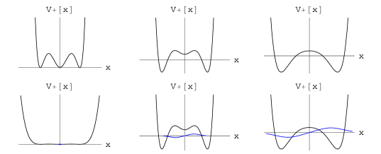
Figure 6: Potential energy $V_{+}(x)$ and wave function $\Psi_{+}^{E_{1}^{+}}(x)$ (blue) as a function of $x$

for several values of $\bar{\hbar}$: (a) ${\bar{\hbar}}=0.001$, (b) ${\bar{\hbar}}=0.1$, (c) ${\bar{\hbar}}=1$.

3. Zero-energy ground state. The dependence of $\Psi_{0}^{G}(x)={\rm exp}[-{({x^{4}\over 4}-{x^{2}\over 2})\over\bar{\hbar}}]$ on $\bar{\hbar}$ is somewhat involved and can be described analytically through the asymptotic behavior when $\bar{\hbar}\rightarrow\bar{\hbar}_{c}$ and $\bar{\hbar}_{c}=0$ is the classical value:

$${\rm exp}[-\frac{1}{2\bar{\hbar}}({x^{4}\over 2}-x^{2})]\simeq\lim_{\bar{\hbar}_{c}\rightarrow 0}{\rm exp}[-\frac{1}{\bar{\hbar}_{c}}({x^{4}\over 2}-x^{2})]\left\{1+{1\over\bar{\hbar}_{c}^{2}}\cdot\left(\frac{2\bar{\hbar}}{({x^{4}\over 2}-x^{2})}-\bar{\hbar}_{c}\right)\right.$$

$$+ \left.\frac{1-2\bar{\hbar}_{c}}{2\bar{\hbar}_{c}^{4}}\cdot\left(\frac{2\bar{\hbar}}{({x^{4}\over 2}-x^{2})}-\bar{\hbar}_{c}\right)^{2}+\frac{1+6\bar{\hbar}_{c}(\bar{\hbar}_{c}-1)}{6\bar{\hbar}_{c}^{6}}\cdot\left(\frac{2\bar{\hbar}}{({x^{4}\over 2}-x^{2})}-\bar{\hbar}_{c}\right)^{3}+\cdots\right\}\qquad.$$

The norm of the BPS ground state $\Psi_{0}^{G}(x)$ is again a non-Gaussian integral. Denoting $z={x-1\over\sqrt{\bar{\hbar}}}$, $2z=\varphi$ and ${3\over 4}\bar{\hbar}=\beta$, we obtain:

$$N(\bar{\hbar})=\int\,dx\,{\rm exp}\left\{-\frac{x^{4}}{2\bar{\hbar}}+\frac{x^{2}}{\bar{\hbar}}\right\}=e^{\bar{\hbar}\over 2}\sqrt{\bar{\hbar}}\int\,dz\,{\rm exp}\left\{-\frac{\bar{\hbar}z^{4}}{2}-2\sqrt{\bar{\hbar}}z^{3}-2z^{2}\right\}\qquad.$$ (24)

$N(\bar{\hbar})={\cal Z}(\bar{\hbar})$ is the partition function for the Euclidean $\lambda(\varphi)^{4}_{0}$-model with spontaneous $x\rightarrow-x$ symmetry breaking in (0+0)-space time dimensions and the Lagrangian:

$$L=-{1\over 2}\varphi^{2}-{\beta\over 4!}\varphi^{4}-{\sqrt{3\beta}\over 3!}\varphi^{3}\qquad.$$ (25)

Performing infinite Gaussian integrals

$${{\cal Z}[\beta]\over e^{2\beta\over 3}\sqrt{4\beta/3}}=\sum_{m=0}^{\infty}\sum_{2k=0}^{\infty}\int{(-\beta)^{m}\over(4!)^{m}m!}\cdot{(-\sqrt{3\beta})^{2k}\over(3!)^{2k}(2k)!}\ \ \varphi^{4m+6k}\ \ e^{-{1\over 2}\varphi^{2}}\ d\varphi$$

one obtains the asymptotic $\bar{\hbar}$-expansion:

$${{\cal Z}[\beta]\over e^{2\beta\over 3}\sqrt{2\beta\pi/3}}=\sum_{m=0}^{\infty}\sum_{k=0}^{\infty}{(-\beta)^{m}\over(4!)^{m}m!}\cdot{(-\sqrt{3\beta})^{2k}\over(3!)^{2k}(2k)!}\cdot{(4m+6k)!\over(2m+3k)!2^{2m+3k}}$$ (26)

$$=1\underbrace{-{\beta\over 8}+{5\cdot 7\over 2^{7}\cdot 3}\beta^{2}-{5\cdot 7\cdot 11\over 2^{10}\cdot 3}\beta^{3}+\cdots}\underbrace{-{3\cdot 5\cdot 7\over 2^{6}}\beta^{2}}+\cdots+\underbrace{{5\over 2^{3}}\beta+{5\cdot 7\cdot 11\over 2^{7}}\beta^{2}+{5\cdot 7\cdot 11\cdot 13\cdot 17\over 2^{10}\cdot 3}\beta^{3}+\cdots}$$

Again, the optimum value of the number of terms of $k$ type can be estimated. Keeping a fixed but finite value of $m=m_{0}$ such that $m_{0}<<k_{0}$, the quotient between two consecutive $k=k_{0}$ and $k=k_{0}+1$ terms must be of the order of one:

$$\left|{a_{m_{0}+k_{0}+1}\over a_{m_{0}+k_{0}}}\right| = \frac{1}{(2k_{0}+2)(2k_{0}+1)}\cdot\left[\frac{(4m_{0}+6k_{0}+6)(4m_{0}+6k_{0}+5)\cdots(4m_{0}+6k_{0}+1)}{(2m_{0}+3k_{0}+3)(2m_{0}+3k_{0}+2)(2m_{0}+3k_{0}+1)}\right]\frac{|3\beta|}{(3!)^{2}2^{3}}$$

$$\approx 27\beta k_{0}\approx 1\Rightarrow k_{0}\approx{1\over 27\beta}\qquad,$$

and the error assumed by neglecting higher-order terms is bounded by ${\rm exp}[-{1\over 27\beta}]$.

Writing the partition function in the form

$${{\cal Z}[\beta]\over e^{2\beta\over 3}\sqrt{4\beta/3}}=\sum_{m=0}^{\infty}\sum_{k=0}^{\infty}\int\overbrace{{(-\beta)\varphi^{4}\over(4!)}\times\cdots\times{(-\beta)\varphi^{4}\over 4!}\over m!}\cdot\overbrace{{(-\sqrt{3\beta})\varphi^{3}\over 3!}\times\cdots\times{(-\sqrt{3\beta})\varphi^{3}\over 3!}\over(2k)!}e^{-{1\over 2}\varphi^{2}}d\varphi$$ (27)

one sees that the Feynman rules encompass one tetra-valent vertex and one trivalent vertex that are proportional respectively to $(-\beta)$ and $-(\sqrt{3\beta})$. Four-leg vertices come from ${(-\beta)\varphi^{4}\over(4!)}$ in the integrand of (27); three-leg vertices are due to ${(-\sqrt{3\beta})\varphi^{3}\over 3!}$ terms in (27) and only contribute in pairs. Comparison with the $\bar{\hbar}$-expansion (26) shows that pictures of the $k=0$ terms, collected in the first two blocks of the first row, are provided by the diagrams shown in Table 1. Diagrams with one tetra-valent and two three-valent vertices, $k=m=1$, shown in Table 2, provide the second block in the first row: $-{3\beta^{2}\over 2^{6}}-{3\beta^{2}\over 3\cdot 2^{5}}-{3\beta^{2}\over 2^{4}}-{3\beta^{2}\over 2^{2}}-{3\beta^{2}\over 2^{3}}-{3\beta^{2}\over 3\cdot 2^{2}}\equiv-{3\cdot 5\cdot 7\over 2^{6}}\beta^{2}$.

Diagram		Weight	Diagram		Weight
	$\rightarrow$	${\displaystyle-{3\beta^{2}\over 2^{6}}}$		$\rightarrow$	${\displaystyle-{3\beta^{2}\over 3\cdot 2^{5}}}$
	$\rightarrow$	${\displaystyle-{3\beta^{2}\over 2^{4}}}$		$\rightarrow$	${\displaystyle-{3\beta^{2}\over 2^{2}}}$
	$\rightarrow$	${\displaystyle-{3\beta^{2}\over 2^{3}}}$		$\rightarrow$	${\displaystyle-{3\beta^{2}\over 3\cdot 2^{2}}}$

,

In Table 3 only diagrams with tri-valent vertices, $m=0$, are displayed:

Vacuum graph		Weight	Vacuum graph		Weight
	$\rightarrow$	${\displaystyle 3\beta\over\displaystyle 2^{3}}$		$\rightarrow$	${\displaystyle 3\beta\over\displaystyle 3\cdot 2^{2}}$
	$\rightarrow$	${\displaystyle 3^{2}\beta^{2}\over\displaystyle 2^{7}}$		$\rightarrow$	${\displaystyle 3^{2}\beta^{2}\over\displaystyle 3\cdot 2^{5}}$
	$\rightarrow$	${\displaystyle 3^{2}\beta^{2}\over\displaystyle 3^{2}\cdot 2^{5}}$		$\rightarrow$	${\displaystyle 3^{2}\beta^{2}\over\displaystyle 2^{5}}$
	$\rightarrow$	${\displaystyle 3^{2}\beta^{2}\over\displaystyle 3\cdot 2^{4}}$		$\rightarrow$	${\displaystyle 3^{2}\beta^{2}\over\displaystyle 2^{4}}$
	$\rightarrow$	${\displaystyle 3^{2}\beta^{2}\over\displaystyle 2^{5}}$		$\rightarrow$	${\displaystyle 3^{2}\beta^{2}\over\displaystyle 3\cdot 2}$

Diagrams with two tri-valent vertices contribute: ${3\beta\over 2^{3}}+{3\beta\over 3\cdot 2^{2}}\equiv{5\over 2^{3}}\beta$, whereas the contribution of diagrams with four trivalent vertices is: ${3^{2}\beta^{2}\over 2^{7}}+{3^{2}\beta^{2}\over 3\cdot 2^{5}}+{3^{2}\beta^{2}\over 2^{5}}+{3^{2}\beta^{2}\over 3\cdot 2^{4}}+{3^{2}\beta^{2}\over 2^{4}}+{3^{2}\beta^{2}\over 2^{5}}+{3^{2}\beta^{2}\over 3\cdot 2}\equiv{5\cdot 7\cdot 11\over 2^{7}}\beta^{2}$.

4 Supersymmetric WKB approximation

The semiclassical regime is characterized by the inequality:

$$\bar{\hbar}\left|{d^{2}W\over dx^{2}}(x)\right|<<\left|{dW\over dx}(x)\right|^{2}=|\Omega(x)\cdot\Omega(x)|^{2}\qquad,\qquad\Omega(x)=\sqrt{2V(x)}\hskip 76.82234pt\quad.$$

Thus,

$${\bar{\lambda}\over 2\pi}={\bar{\hbar}\over\sqrt{2V(x)}}<<\left|\frac{2V(x)}{dV/dx}\right|$$

is satisfied in the limit of short wave lengths. To obtain the WKB eigen-functions of the SUSY Hamiltonian in, e.g. , the subspace for which the zero Fermi number is zero - because supersymmetry WKB eigenfunctions of non-zero energy in the Fermi sector are given automatically - one starts from the Wentzel-Krammers-Brillouin ansatz in the classically forbidden region $E<V(x)$:

$$\Psi^{E}(x,t)=A(x)\cdot{\rm exp}[-\frac{W_{E}(x)}{\bar{\hbar}}]\cdot e^{i\frac{Et}{\bar{\hbar}}}\qquad.$$ (28)

The Schrodinger equation for $V_{+}(x)$ becomes

$$\bar{\hbar}^{2}\left({d^{2}\ln A\over dx^{2}}(x)+{d\ln A\over dx}(x)\cdot{d\ln A\over dx}(x)\right)-$$ (29)

$$- \bar{\hbar}\left({d^{2}W_{E}\over dx^{2}}(x)+2\ln A(x)\cdot{dW_{E}\over dx}(x)-{d\Omega\over dx}(x)\right)+W_{E}(x)\cdot W_{E}(x)-\Omega(x)\cdot\Omega(x)+2E=0\quad.$$

with three terms of respectively order 2,1, and 0 in $\bar{\hbar}$. The usual WKB strategy starts by solving the equation (29) for the $\bar{\hbar}$-independent terms to find:

$$W_{E}(x)=\int\,dx\,\sqrt{\Omega(x)\cdot\Omega(x)-2E}\qquad,$$

with the novelty with respect to the non SUSY case that the turning points are those corresponding to $V(x)$, rather than those set by the effective potential $V_{+}(x)$. The second step is to plug this solution into the equation for the terms proportional to $\bar{\hbar}$:

$$\frac{d\ln A}{dx}(x)={1\over 2}\left[\frac{1}{\sqrt{\Omega(x)\Omega(x)-2E}}-\frac{\Omega(x)}{\Omega(x)\Omega(x)-2E}\right]\cdot{d\Omega\over dx}(x)\qquad.$$

Integration of this equation provides the SUSY WKB wave functions:

$$A(x)\propto\frac{1}{(\Omega(x)\Omega(x)-2E)^{{1\over 4}}}\cdot\left(|\Omega|(x)+\sqrt{\Omega(x)\Omega(x)-2E}\right)^{{|\over 2}}\qquad.$$ (30)

Note the other difference: in the non-SUSY case the numerator of this expression is $1$. In the classical allowed regions, $2E>\Omega^{2}(x)$, however, the WKB ansatz reads,

$$\psi^{E}(x)=A(x){\rm exp}[-i\frac{|W(x)|}{\bar{\hbar}}]\qquad,$$ (31)

and one obtains:

$$A(x)={1\over\left[2E-\Omega^{2}(x)\right]^{{1\over 4}}}\cdot{\rm exp}\left[{i\over 2}{\rm arcsin}\frac{\Omega(x)}{\sqrt{2E}}\right]\qquad.$$

To match the WKB wave functions (28) and (31) analytically at the classical turning points $x=a\,<\,x=b$, such that $\Omega^{2}(a)=2E=\Omega^{2}(b)$, the following supersymmetric quantization rule is required:

$$\int_{a}^{b}\,dx\,\left[2E-\Omega^{2}(x)\right]^{{1\over 2}}=n\pi\bar{\hbar}\qquad\qquad n\in{\mathbb{Z}}^{+}\qquad.$$ (32)

The appearance of the numerator in (30) is magic: firstly, because this term modifies the process of analytic continuation necessary to match the exponential and periodic WKB wave functions at the turning points in such a way that the ${\pi\over 2}\bar{\hbar}$ term that appears in the non SUSY version of (32) does not enter the SUSY case. To obtain the WKB wave function in the classically allowed region

$$\psi^{E}(x)=e^{-\sqrt{{E\over 2}}}\cdot\frac{\sqrt{\sqrt{2E-\Omega^{2}}+i\Omega}}{(2E-\Omega^{2})^{1\over 4}}\cdot\left\{C_{1}e^{{i\over\bar{\hbar}}\int_{b}^{x}\,dx^{\prime}\,\sqrt{2E-\Omega^{2}(x^{\prime})}}+C_{2}e^{-{i\over\bar{\hbar}}\int_{b}^{x}\,dx^{\prime}\,\sqrt{2E-\Omega^{2}(x^{\prime})}}\right\}$$

from the WKB wave functions in the forbidden regions

$$\psi^{E}(x)=C\frac{\sqrt{\sqrt{\Omega^{2}-2E}+|\Omega|}}{(\Omega^{2}-2E)^{1\over 4}}\cdot e^{-{1\over\bar{\hbar}}\int_{x}^{a}\,dx^{\prime}\,\sqrt{\Omega^{2}(x^{\prime})-2E}}\hskip 4.26773pt;\hskip 4.26773pt\psi^{E}(x)=C^{\prime}\frac{\sqrt{\sqrt{\Omega^{2}-2E}+|\Omega|}}{(\Omega^{2}-2E)^{1\over 4}}\cdot e^{-{1\over\bar{\hbar}}\int_{b}^{x}\,dx^{\prime}\,\sqrt{\Omega^{2}(x^{\prime})-2E}}$$

one chooses paths in the $x$-complex plane that goes around the turning points $a$ and $b$ at great distance, either in the upper or the lower half-planes. Unlike to the non-SUSY case, there is no $e^{-i{\pi\over 4}}$ factor left and two wave functions are obtained in the classically allowed region, one from the left and the other from the right:

$$\psi^{E}(x)=C\frac{\sqrt{\sqrt{2E-\Omega^{2}(x)}+i\Omega(x)}}{(2E-\Omega^{2}(x))^{1\over 4}}\cdot{\rm cos}[{1\over\bar{\hbar}}\int_{b}^{x}\,dx^{\prime}\,\sqrt{2E-\Omega^{2}(x^{\prime})}]$$

$$\psi^{E}(x)=C^{\prime}\frac{\sqrt{\sqrt{2E-\Omega^{2}(x)}+i\Omega(x)}}{(2E-\Omega^{2}(x))^{1\over 4}}\cdot{\rm cos}[{1\over\bar{\hbar}}\int_{x}^{a}\,dx^{\prime}\,\sqrt{2E-\Omega^{2}(x^{\prime})}]\qquad.$$

These expressions are identical if and only if (32) holds. Secondly, $E=0$ is a solution of (32) for $n=0$, whereas (28) becomes the exponential of the superpotential: the exact ground state is a SUSY WKB wave function !

4.1 WKB analysis of the single well

We shall consider as examples non-harmonic oscillators of fourth order to avoid hyperelliptic integrals and deal with (slightly!) manageable expressions. In the case of a single well with potential energy $V(x)={\lambda\over 2}(x^{2}+{k\over\lambda})^{2}$ we have, using non-dimensional variables:

$$V(x)={1\over 2}(x^{4}+2x^{2}+1)\qquad,\qquad\Omega(x)=x^{2}+1\qquad,\qquad W(x)={x^{3}\over 3}+x\qquad.$$

The turning points are the real roots of the quartic equation:

$$x^{4}+2x^{2}-a=0\qquad,\qquad a=2E-1\qquad,\qquad x_{\pm}=\pm\sqrt{-1+\sqrt{1+a}}\qquad.$$ (33)

The supersymmetric quantization rule is therefore:

$$I(E;x_{-},x_{+})=\int_{x_{-}}^{x_{+}}\sqrt{a-x^{4}-2x^{2}}\,dx=n\pi\bar{\hbar}\qquad.$$ (34)

Denoting $A_{\pm}=\pm 1+\sqrt{1+a}$, the definite integral in (37) reads:

$$I(E;x_{-},x_{+})=\frac{4}{3}\sqrt{A_{-}}\left(\sqrt{a+1}\,\mathbb{K}\left(\frac{-A_{-}}{A_{+}}\right)-\mathbb{E}\left(\frac{-A_{-}}{A_{+}}\right)\right)\qquad,$$ (35)

where $\mathbb{K}(k^{2})$ and $\mathbb{E}(k^{2})$ are respectively the complete elliptic integrals of first and second type. This result is shown in Figure 8.

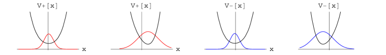
Figure 7: Graphics of $V^{\pm}(x)$ for $\bar{\hbar}=0.1$ -(1),(3)- and $\bar{\hbar}=1$ -(2),(4)-.

     

Figure 8: Mathematica plot of $I(E;x_{-},x_{+})$ as a function of $a$ and intersection with $n\pi\bar{\hbar}$ for low $n$ and $\bar{\hbar}=1$ (left) and $\bar{\hbar}=0.1$ (right)

The first three (double, see Figure 7) eigenvalues for $\bar{\hbar}=1$ and $\bar{\hbar}=0.1$ are: $E_{1}=2.18674{k^{2}\over\lambda}$, $E_{2}=4.23942\,{k^{2}\over\lambda}$, $E_{3}=6.5444\,{k^{2}\over\lambda}$, and $E_{1}=0.64500\,{k^{2}\over\lambda}$, $E_{2}=0.78289\,{k^{2}\over\lambda}$, $E_{3}=0.95403\,{k^{2}\over\lambda}$, respectively.

4.2 WKB analysis of the double well

For a non-harmonic oscillator of fourth order and a double well things are even more difficult. The potential energy is $V(x)={\lambda\over 2}(x^{2}-{k\over\lambda})^{2}$, such that in non-dimensional variables we have:

$$V(x)={1\over 2}(x^{4}-2x^{2}+1)\qquad,\qquad\Omega(x)=x^{2}-1\qquad,\qquad W(x)={x^{3}\over 3}-x\qquad.$$

The turning points are the real solutions of the quartic equation:

$$x^{4}-2x^{2}-a=0\qquad,\qquad x_{-\,\mp}=-\sqrt{1\mp\sqrt{1+a}}\qquad,\qquad x_{+\,\mp}=\sqrt{1\mp\sqrt{1+a}}\qquad.$$ (36)

For $a>0$ there are only two real roots and the supersymmetric quantization rule reads:

$$I(E;x_{-+},x_{++})=\int_{x_{-+}}^{x_{++}}\sqrt{a-x^{4}+2x^{2}}\,dx=n\pi\bar{\hbar}\qquad.$$ (37)

The computation of $I(E;x_{-+},x_{++})$ is qualitatively identical to the previous case and results are shown in Fig. 10(left).

If $-1<a<0$ things are more difficult: there are four turning points, four real roots, and the quantization rule splits into two equations:

$$I(E;x_{--},x_{+-})=\int_{x_{--}}^{x_{+-}}\sqrt{a-x^{4}+2x^{2}}\,dx=n\pi\bar{\hbar}=I(E;x_{-+},x_{++})=\int_{x_{-+}}^{x_{++}}\sqrt{a-x^{4}+2x^{2}}\,dx\quad.$$ (38)

The definite integrals in (38) now read:

$$I(E;x_{--},x_{+-})=I(E;x_{-+},x_{++})= \frac{2a}{3A_{+}\sqrt{A_{-}}}\left[\sqrt{a+1}\,\left(\mathbb{K}\left(\frac{-A_{+}}{A_{-}}\right)-\mathbb{F}\left(\arcsin\sqrt{\frac{-A_{-}}{A_{+}}},\frac{-A_{+}}{A_{-}}\right)\right)\right.$$ (39)

$$\left.-\mathbb{E}\left(\frac{-A_{-}}{A_{+}}\right)+\mathbb{E}\left(\arcsin\sqrt{\frac{-A_{-}}{A_{+}}},\frac{-A_{+}}{A_{-}}\right)\right]\qquad.$$

Note that incomplete elliptic integrals of the first, ${\mathbb{F}}(u,m)$, and second, ${\mathbb{K}}(u,m)$, type also enter. In any case, it is possible to plot these functions of $a$ and find the intersection points determining the spectrum.

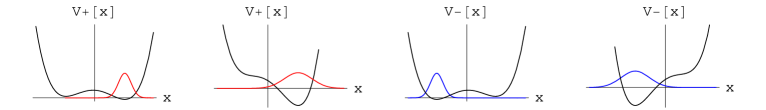
Figure 9: Graphics of $V^{\pm}(x)$ for $\bar{\hbar}=0.1$ -(1),(3)- and $\bar{\hbar}=1$ -(2),(4)-.

     

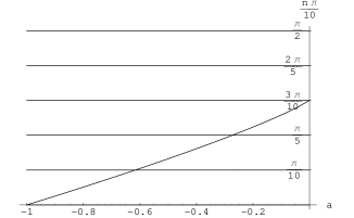
Figure 10: Mathematica plots of $I(E;x_{-+},x_{++})$ for $\bar{\hbar}=1$ and $a>0$ (left) and $I(E;x_{--},x_{+-})$ for $\bar{\hbar}=0.1$ and $-1<a<0$ (right) as function of $a$. The intersection points with $n\pi\bar{\hbar}$ giving the eigenvalues are also shown.

The first three eigenvalues for $a>0$ and $\bar{\hbar}=1$ are: $E_{1}=0.82272\,{k^{2}\over\lambda}$, $E_{2}=2.08330\,{k^{2}\over\lambda}$, $E_{3}=5.63830\,{k^{2}\over\lambda}$.

In the case of $-1<a<0$ eigenvalues only exist if $\bar{\hbar}<0.95$. Application of rule (38) for the turning points on the left gives: $E_{1}=0.19183\,{k^{2}\over\lambda}$, $E_{2}=0.36384\,{k^{2}\over\lambda}$, $E_{3}=0.49993\,{k^{2}\over\lambda}$.

Because of formula (39) the choice of pair of turning points is irrelevant; $E_{1}$, $E_{2}$, $E_{3}$, etcetera, are eigenvalues of the Schrödinger equation for both $V_{+}(x)$ and $V_{-}$.

5 Outlook

The next step is to study physical systems of two degrees of freedom. It is tempting to start by discussing problems of this type in Hamilton separable systems. Following the works [15]-[16] on supersymmetric quantum mechanics in more than one dimensions, the general structure of supersymmetric classical and quantum Liouville systems has been described in References [14] and [13]. An important example of this kind of systems is the supersymmetric classical and quantum hydrogen atom respectively analyzed by Heumann [18] and Kirchberg et al [19]. It seems also plausible to address similar issues in non-separable but integrable systems as those proposed in [20].

6 Acknowledgements

We thank M. Ioffe for enlightening conversations on supersymmetric quantum mechanics and a critical reading of the manuscript. This work has been partially supported by the Spanish MEC grant BFM2003-00936 and the project VA013C05 of the Junta de Castilla y Leon.

References

- [1]
- [2] J. F. Cariena, Motion on Lie Groups and Applications in Classical and Quantum Mechanics, Anales de Fisica, Monografias 6 (2002)211-226, Real Sociedad Espa ola de Fisica
- [3] J. F. Cariena and J. Ramos, Reviews in Math. Phys. A12 (2000) 1279-1304
- [4] J. F. Cariena, D. J. Fernandez, and J. Ramos, Ann. Phys. 292 (2001) 42
- [5] F. Cooper, A. Khare and U. Sukhatme, Phys: Rep.25(1995) 268
- [6] G. Junker, Supersymmetric methods in quantum and statistical physics, Springer Verlag, Berlin, 1996
- [7] A. Wipf, Non-perturbative methods in supersymmetric theories, hep-th/0504180
- [8] H. Goldstein, Classical Mechanics, Addison -Wesley, Reading, Massachusetts, 1980
- [9] R. Casalbuoni, Nuovo Cimento 33A (1976)115
- [10] N.V.Borisov, M.I.Eides, M.V.Ioffe Theor.Math.Phys. 29 (1976)906
- [11] R. Borcherds and A. Barnard, Lectures on Quantum Field Theory, math-phys/0204014
- [12] A. Comtet, D. Bandrauk and D. Campbell, Phys. Lett. B150 (1985) 159
- [13] A. Alonso, M.A. González, M. de la Torre and J. Mateos Guilarte, J. Phys. A 37 (2004) 10323.
- [14] A. Alonso, M.A. González, J. Mateos Guilarte and M. de la Torre, Ann. Phys. 308 (2003) 664.
- [15] A.A. Andrianov, N.V. Borisov. M.I. Eides and M. V. Ioffe, Phys. Lett A109 (1985) 143.
- [16] A.A. Andrianov, N.V. Borisov. M.I. Eides and M.V. Ioffe, Theor. Math. Phys. 61 (1984) 963.
- [17] P.F. Byrd and M.D. Friedman, Handbook of Elliptic Integrals for Engineers and Scientist, Springer-Verlag 1971.
- [18] R. Heumann, J. Phys. A 35 (2002) 7437.
- [19] A. Kirchberg, J.D. Länge, P.A.G. Pisani and A. Wipf, Ann. Phys. 303 (2003) 359.
- [20] M.V. Ioffe, J. Mateos Guilarte, and P.A. Valinevich, Two-dimensional supersymmetry: from susy quantum mechanics to classically integrable models, Ann. Phys., to appear, hep-th/0603006.