Emissivities for the various Graviton Modes in the Background of the Higher-Dimensional Black Hole

Abstract

The Hawking emissivities for the scalar-, vector-, and tensor-mode bulk gravitons are computed in the full range of the graviton’s energy by adopting the analytic continuation numerically when the spacetime background is $(4+n)$-dimensional non-rotating black hole. The total emissivity for the gravitons is only $5.16\%$ of that for the spin-$0$ field when there is no extra dimension. However, this ratio factor increases rapidly when the extra dimensions exist. For example, this factor becomes $147.7\%$, $595.2\%$ and $3496\%$ when the number of extra dimensions is $1$, $2$ and $6$, respectively. This fact indicates that the Hawking radiation for the graviton modes becomes more and more significant and dominant with increasing the number of extra dimensions.

Recent quantum gravity such as string theories[1] or brane-world scenario[2] generally requires the extra dimensions to reconcile general relativity with quantum physics. Especially the modern brane-world scenarios predict the emergence of the TeV-scale gravity, which opens the possibility to make tiny black holes by high-energy scattering in the future colliders[3]. In this reason much attention is paid recently to the effect of the extra dimensions in the black hole physics.

The absorption problem and Hawking radiation for the spin $0$, $1/2$ and $1$ particles in the background of the $(4+n)$-dimensional Schwarzschild black hole were explored in Ref.[4]. The numerical calculation supports the fact that the black holes radiate mainly on the brane. In fact this was pointed out by Emparan, Horowitz and Myers(EHM) in Ref.[5] by making use of the higher-dimensional black body radiation. This claim was also supported in the background of the higher-dimensional charged black hole[6].

More recently, this issue was re-examined when the situation is different. If, for example, black hole has a rotation, there is an important factor we should consider carefully called superradiance[7]. The superradiance in the background of the higher-dimensional black hole was examined for the bulk fields[8] and brane fields[9]. However, numerical calculation has shown that in spite of the consideration of the superradiance EHM claim still holds due to the incrediably large difference in the energy amplification for the brane field and bulk field[10].

There is an another factor we have not considered thoroughly. This is an Hawking radiation for the higher-spin particles like graviton. Since the graviton is not generally localized on the brane unlike the usual standard model particles, the argument of EHM should be carefully re-checked in the graviton emission. Generalizing the Regge-Wheeler method[11], the various gravitational perturbations were studied in Ref.[12] in the background of the higher-dimensional Schwarzschild black hole. Using the radial equations derived in Ref.[12], the low-energy and high-energy behaviors for the bulk graviton absorption and emission spectra were recently studied[13]. The graviton emission on the brane is also examined using an axial perturbation[14]. In Ref.[14] it was argued that the graviton emission can be dominant one in the Hawking radiation when there are many extra dimensions. We would like to explore this issue again in the bulk emission. In the following we will compute the absorption and emission spectra for the various graviton modes numerically. We will show the emission rates are generally enhanced when the number of extra dimensions,say $n$, increases. However, the increasing rate for the gravitons is much larger than that for the spin-$0$ field. For example, the total emissivities for the gravitons is only $5.16\%$ of that for the spin-$0$ field in four dimensions. However, this ratio becomes $595.2\%$ when $n=2$ and $3496\%$ when $n=6$. Thus the Hawking radiation for the higher-spin fields becomes dominant when the extra dimensions exist.

We start with $(4+n)$-dimensional Schwarzschild spacetime whose metric is

$$ds^{2}=-hdt^{2}+h^{-1}dr^{2}+r^{2}d\Omega_{n+2}^{2}$$ (1)

where $h=1-(r_{H}/r)^{n+1}$ and the angle part $d\Omega_{n+2}^{2}$ is a spherically symmetric line element in a form

$$d\Omega_{n+2}^{2}=d\theta_{n+1}^{2}+\sin^{2}\theta_{n+1}\Bigg{[}d\theta_{n}^{2}+\sin^{2}\theta_{n}\bigg{(}\cdots+\sin^{2}\theta_{2}\left(d\theta_{1}^{2}+\sin^{2}\theta_{1}d\varphi^{2}\right)\cdots\bigg{)}\Bigg{]}.$$ (2)

It is well-known[12] that when $n\neq 0$, there are three gravitational metric perturbations, i.e. scalar, vector and tensor perturbations. For the vector and tensor modes the radial equation reduces to the following Schrödinger-like expression

$$\left(\frac{d^{2}}{dr_{\ast}^{2}}+\omega^{2}\right)\Psi=V_{VT}\Psi$$ (3)

where $r_{\ast}$ is a “tortoise” coordinate defined $dr/dr_{\ast}=h$ and the effective potential $V_{VT}$ is

$$V_{VT} = \frac{h}{r^{2}}\left[\ell(\ell+n+1)+\frac{n(n+2)}{4}-\frac{k(n+2)^{2}}{4}\left(\frac{r_{H}}{r}\right)^{n+1}\right]$$ (7)

$$k=\left\{\begin{array}[]{ll}-1&\mbox{for tensor mode}\\ 3&\mbox{for vector mode}\end{array}\right.$$

with $\ell\geq 2$.

The radial equation for the scalar mode also reduces to the Schrödinger-like expression. However, the effective potential $V_{S}$ is comparatively complicate as following

$$V_{S}=\frac{h}{r^{2}}\frac{qy^{3}+py^{2}+wy+z}{4[2m+(n+2)(n+3)y]^{2}}$$ (8)

where $y=1-h=(r_{H}/r)^{n+1}$ and

$$m = \ell(\ell+n+1)-(n+2)\hskip 56.9055ptq=(n+2)^{4}(n+3)^{2}$$ (9)

$$z = 16m^{3}+4m^{2}(n+2)(n+4)$$ (10)

$$p = (n+2)(n+3)\left[4m(2n^{2}+5n+6)+n(n+2)(n+3)(n-2)\right]$$ (11)

$$w = -12m(n+2)\left[m(n-2)+n(n+2)(n+3)\right]$$ (12)

with $\ell\geq 2$.

In the $4d$ limit the vector mode corresponds to the gravitational axial perturbation[15], whose effective potential reduces to

$$V_{A}(r)=\frac{h}{r^{2}}\left[(2\lambda+2)-3\left(\frac{r_{H}}{r}\right)\right],$$ (13)

and the scalar mode corresponds to the gravitational polar perturbation[16] with

$$V_{P}(r)=\frac{h}{(2\lambda r+3r_{H})^{2}}\left[8\lambda^{2}(\lambda+1)+12\lambda^{2}\left(\frac{r_{H}}{r}\right)+18\lambda\left(\frac{r_{H}}{r}\right)^{2}+9\left(\frac{r_{H}}{r}\right)^{3}\right]$$ (14)

where $\lambda=(\ell-1)(\ell+2)/2$. There is no correspondence of the tensor mode in four dimension. The most striking result in the $4d$ gravitational metric perturbations is the fact that the effective potentials $V_{A}$ and $V_{P}$, which look completely different from each other, are expressed as a single equation[17]

$$V_{P,A}(r)=\pm\beta\frac{df}{dr_{*}}+\beta^{2}f^{2}+\kappa f$$ (15)

where $\beta=3r_{H}$, $\kappa=4\lambda(\lambda+1)$ and $f=h/r(2\lambda r+3r_{H})$. In fact, this relation was found when Newman-Penrose formalism[18] is applied to the $4d$ gravitational perturbations. Making use of this explicit relation, one can show that the effective potentials $V_{A}$ and $V_{P}$ have the same transmission coefficient. This fact also indicates that the absorption and emission spectra for the vector mode graviton and scalar mode graviton by a Schwarzschild black hole are exactly same in four dimensions.

Now, we would like to discuss how the absorption and emission spectra are computed. We first consider the vector and tensor modes of the bulk graviton. Defining the dimensionless parameters $x\equiv\omega r$ and $x_{H}\equiv\omega r_{H}$, one can rewrite Eq.(3) in the following

$$4x^{2}\left(x^{n+1}-x_{H}^{n+1}\right)^{2}\frac{d^{2}\Psi}{dx^{2}}+4(n+1)x_{H}^{n+1}x\left(x^{n+1}-x_{H}^{n+1}\right)\frac{d\Psi}{dx}$$ (16)

$$+\left[4x^{2n+4}-\left(x^{n+1}-x_{H}^{n+1}\right)\left\{(2\ell+n)(2\ell+n+2)x^{n+1}-k(n+2)^{2}x_{H}^{n+1}\right\}\right]\Psi=0.$$ (17)

One can easily show that if $\Psi$ is a solution of Eq.(16), its complex conjugate $\Psi^{\ast}$ is also solution. Eq.(16) also guarantees the Wronskian between them is

$$W[\Psi^{\ast},\Psi]_{x}\equiv\Psi^{\ast}\frac{d\Psi}{dx}-\Psi\frac{d\Psi^{\ast}}{dx}=\frac{{\cal C}x^{n+1}}{x^{n+1}-x_{H}^{n+1}}$$ (18)

where ${\cal C}$ is an integration constant.

Now, we would like to consider the solution of Eq.(16), which is convergent in the near-horizon regime, i.e. $x\sim x_{H}$. Since $x=x_{H}$ is a regular singular point, this solution can be derived by a series expression as following

$${\cal G}_{n,\ell}(x,x_{H})=e^{\lambda_{n}\ln|x-x_{H}|}\sum_{N=0}^{\infty}d_{\ell,N}(x-x_{H})^{N}.$$ (19)

Inserting Eq.(19) into (16) easily yields

$$\lambda_{n}=-i\frac{x_{H}}{n+1}.$$ (20)

The sign of $\lambda_{n}$ is chosen for the near-horizon solution to be ingoing into the black hole. The recursion relation for the coefficients $d_{\ell,N}$ can be obtained too. Since it is ,of course, $n$-dependent and lengthy, we will not present it here. The Wronskian (18) enables us to derive

$$W[{\cal G}_{n,\ell}^{\ast},{\cal G}_{n,\ell}]_{x}=\frac{-2i|g_{n,\ell}|^{2}x^{n+1}}{x^{n+1}-x_{H}^{n+1}}$$ (21)

where $g_{n,\ell}\equiv d_{\ell,0}$.

Next, we would like to discuss the solution of Eq.(16), which is convergent in the asymptotic regime. This is also expressed as a series form by inverse power of $x$ as following:

$${\cal F}_{n,\ell(\pm)}(x,x_{H})=(\pm i)^{\ell+1+\frac{n}{2}}xe^{\mp ix}(x-x_{H})^{\pm\lambda_{n}}\sum_{N=0}^{\infty}\tau_{N(\pm)}x^{-(N+1)}$$ (22)

with $\tau_{0(\pm)}=1$. The solutions ${\cal F}_{n,\ell(+)}$ and ${\cal F}_{n,\ell(-)}$ are respectively the ingoing and outgoing solutions. Using Eq.(18), one can show easily

$$W[{\cal F}_{n,\ell(+)},{\cal F}_{n,\ell(-)}]_{x}=\frac{2ix^{n+1}}{x^{n+1}-x_{H}^{n+1}}.$$ (23)

The recursion relation for the coefficients $\tau_{N(\pm)}$ is straightforwardly derived, which is too lengthy to present here.

Now, we would like to discuss how the coefficient $g_{n,\ell}(\equiv d_{\ell,0})$ is related to the scattering amplitude. Since the real scattering solution, say ${\cal R}_{n,\ell}$ should be ingoing wave in the near-horizon regime and the mixture of ingoing and outgoing waves at the asymptotic regime, one may express it in the form:

$${\cal R}_{n,\ell}\stackrel{{\scriptstyle x\rightarrow x_{H}}}{{\sim}}g_{n,\ell}(x-x_{H})^{\lambda_{n}}\left[1+O(x-x_{H})\right]$$ (24)

$${\cal R}_{n,\ell}\stackrel{{\scriptstyle x\rightarrow\infty}}{{\sim}}\frac{i^{\ell+1+\frac{n}{2}}2^{\frac{n}{2}-1}}{\sqrt{\pi}}\Gamma\left(\frac{1+n}{2}\right)Q_{n,\ell}$$ (25)

$$\hskip 56.9055pt\times\left[e^{-ix+\lambda_{n}\ln|x-x_{H}|}-(-1)^{\ell+\frac{n}{2}}S_{n,\ell}(x_{H})e^{ix-\lambda_{n}\ln|x-x_{H}|}\right]+O\left(\frac{1}{x}\right)$$ (26)

where $S_{n,\ell}(x_{H})$ is a scattering amplitude and $Q_{n,\ell}$ is a quantity related to the multiplicities ${\cal N}_{n,\ell}$ as following:

$$Q_{n,\ell}=\frac{2}{(n+4)(n+1)}{\cal N}_{n,\ell}.$$ (27)

The multiplicities ${\cal N}_{n,\ell}^{(S)}$, ${\cal N}_{n,\ell}^{(V)}$ and ${\cal N}_{n,\ell}^{(T)}$ for the scalar-, vector- and tensor-mode bulk gravitons are given by[13]

$${\cal N}_{n,\ell}^{(S)} = \frac{(2\ell+n+1)(\ell+n)!}{\ell!(n+1)!}$$ (28)

$${\cal N}_{n,\ell}^{(V)} = \frac{\ell(\ell+n+1)(2\ell+n+1)(\ell+n-1)!}{(\ell+1)!n!}$$ (29)

$${\cal N}_{n,\ell}^{(T)} = \frac{n(n+3)(\ell+n+2)(\ell-1)(2\ell+n+1)(\ell+n-1)!}{2(\ell+1)!(n+1)!}.$$ (30)

Introducing a phase shift $\delta_{n,\ell}$ as $S_{n,\ell}\equiv e^{2i\delta_{n,\ell}}$, one can rewrite the second equation of Eq.(24) in the form

$${\cal R}_{n,\ell}\stackrel{{\scriptstyle x\rightarrow\infty}}{{\sim}}\frac{2^{\frac{n}{2}}}{\sqrt{\pi}}\Gamma\left(\frac{1+n}{2}\right)Q_{n,\ell}e^{i\delta_{n,\ell}}$$ (31)

$$\hskip 56.9055pt\times\sin\left[x+i\lambda_{n}\ln|x-x_{H}|-\frac{\pi}{2}\left(\ell+\frac{n}{2}\right)+\delta_{n,\ell}\right]+O\left(\frac{1}{x}\right).$$ (32)

The near-horizon behavior of the real scattering solution, i.e. the first one of Eq.(24), implies that the Wronskian $W[{\cal R}_{n,\ell}^{\ast},{\cal R}_{n,\ell}]_{x}$ is same with Eq.(21). However, Eq.(31) implies

$$[{\cal R}_{n,\ell}^{\ast},{\cal R}_{n,\ell}]_{x}=-i\frac{2^{n}}{\pi}\Gamma^{2}\left(\frac{1+n}{2}\right)Q_{n,\ell}^{2}e^{-2\beta_{n,\ell}}\sinh 2\beta_{n,\ell}\frac{x^{n+1}}{x^{n+1}-x_{H}^{n+1}}$$ (33)

where $\delta_{n,\ell}=\eta_{n,\ell}+i\beta_{n,\ell}$. Equalizing these two Wronskians yields a relation between $g_{n,\ell}$ and $\beta_{n,\ell}$ as following:

$$|g_{n,\ell}|^{2}=\frac{2^{n-2}}{\pi}\Gamma^{2}\left(\frac{1+n}{2}\right)Q_{n,\ell}^{2}\left(1-e^{-4\beta_{n,\ell}}\right).$$ (34)

Thus one can calculate the transimission coefficient $1-|S_{n,\ell}|^{2}=1-e^{-4\beta_{n,\ell}}$ if $g_{n,\ell}$ is known.

Now, we would like to explain how to compute $g_{n,\ell}$. For the explanation it is convenient to introduce a new radial solution $\tilde{{\cal R}}_{n,\ell}(x)$, which differs from ${\cal R}_{n,\ell}(x)$ in its normalization in such a way that

$$\tilde{{\cal R}}_{n,\ell}(x,x_{H})\stackrel{{\scriptstyle x\rightarrow x_{H}}}{{\sim}}(x-x_{H})^{\lambda_{n}}\left[1+O(x-x_{H})\right].$$ (35)

Since ${\cal F}_{n,\ell(\pm)}$ are two linearly independent solutions of Eq.(16), one can express $\tilde{{\cal R}}_{n,\ell}$ as a linear combination of them as following

$$\tilde{{\cal R}}_{n,\ell}(x,x_{H})=f_{n,\ell}^{(-)}(x_{H}){\cal F}_{n,\ell(+)}(x,x_{H})+f_{n,\ell}^{(+)}(x_{H}){\cal F}_{n,\ell(-)}(x,x_{H})$$ (36)

where $f_{n,\ell}^{(\pm)}$ are called jost functions. Using Eq.(23) one can compute the jost functions as following

$$f_{n,\ell}^{(\pm)}(x_{H})=\pm\frac{x^{n+1}-x_{H}^{n+1}}{2ix^{n+1}}W[{\cal F}_{n,\ell(\pm)},\tilde{{\cal R}}_{n,\ell}]_{x}.$$ (37)

Inserting the explicit expressions of ${\cal F}_{n,\ell(\pm)}$ in Eq.(22) into Eq.(36) and comparing it with the second equation of Eq.(24), one can derive the following two relations

$$S_{n,\ell}(x_{H}) = \frac{f_{n,\ell}^{(+)}(x_{H})}{f_{n,\ell}^{(-)}(x_{H})}$$ (38)

$$f_{n,\ell}^{(-)}(x_{H}) = \frac{2^{\frac{n}{2}-1}}{\sqrt{\pi}g_{n,\ell}(x_{H})}\Gamma\left(\frac{1+n}{2}\right)Q_{n,\ell}.$$ (39)

Combining Eq.(34) and (38), one can express the greybody factor(or transmission coefficient) of the black hole in terms of the jost function in the following

$$1-|S_{n,\ell}|^{2}=\frac{1}{|f_{n,\ell}^{(-)}|^{2}}.$$ (40)

The partial absorption cross sections for the vector and tensor graviton modes by the $(4+n)$-dimensional Schwarzschild black hole are given by

$$\sigma_{n,\ell}=2^{n+1}\pi^{(n+1)/2}\Gamma\left(\frac{3+n}{2}\right)Q_{n,\ell}\frac{r_{H}^{n+2}}{x_{H}^{n+2}|f_{n,\ell}^{(-)}|^{2}}.$$ (41)

Applying the Hawking formula[19], one can compute the bulk emission rate, i.e. the energy emitted to the bulk per unit time and unit energy interval, as following

$$\frac{\Gamma}{d\omega}=\left[2^{n+3}\pi^{(n+3)/2}\Gamma\left(\frac{3+n}{2}\right)\right]^{-1}(n+4)(n+1)\frac{\omega^{n+3}\sigma_{abs}(\omega)}{e^{\omega/T_{H}}-1}$$ (42)

where $\sigma_{abs}$ is a total absorption cross section and $T_{H}$ is an Hawking temperature given by $T_{H}=(n+1)/4\pi r_{H}$. Thus one can compute the absorption and emission spectra in the full range of $\omega$ if the jost functions are computed.

One can compute the jost functions by matching the near-horizon and asymptotic solutions. This is achieved by the analytic continuation[6, 10] using a solution of Eq.(16) which is convergent at the arbitrary point $x=b$. This solution is also expressed as a series form as following

$$\varphi_{n,\ell}(x,x_{H})=(x-x_{H})^{\lambda_{n}}\sum_{N=0}^{\infty}D_{N}(x-b)^{N}.$$ (43)

The recursion for the coefficients $D_{N}$ can be obtained by inserting Eq.(43) into (16). Since it is too lengthy, we will not present it here. Using a solution (43) one can increase the convergent region for the asymptotic solution from the near-horizon regime and decrease for the asymptotic solution from the asymptotic regime. Repeating the procedure eventually makes the two solutions which have common convergent region. Then one can compute the jost functions by making use of these two solutions and Eq.(37).

Now, we would like to discuss the case of the scalar mode graviton. Introducing the dimensionless parameters $x=\omega r$ and $x_{H}=\omega r_{H}$ again, one can rewrite the radial equation for the scalar mode as

$$4x^{2}\left(x^{n+1}-x_{H}^{n+1}\right)^{2}\left[2mx^{n+1}+(n+2)(n+3)x_{H}^{n+1}\right]^{2}\frac{d^{2}\Psi}{dx^{2}}$$ (44)

$$+4(n+1)x_{H}^{n+1}x\left(x^{n+1}-x_{H}^{n+1}\right)\left[2mx^{n+1}+(n+2)(n+3)x_{H}^{n+1}\right]^{2}\frac{d\Psi}{dx}$$ (45)

$$\hskip 28.45274pt\Bigg{[}4x^{2n+4}\left[2mx^{n+1}+(n+2)(n+3)x_{H}^{n+1}\right]^{2}$$ (46)

$$\hskip 56.9055pt-\left(x^{n+1}-x_{H}^{n+1}\right)\left\{zx^{3n+3}+wx_{H}^{n+1}x^{2n+2}+px_{H}^{2n+2}x^{n+1}+qx_{H}^{3n+3}\right\}\Bigg{]}\Psi=0.$$ (47)

The calculational procedure is exactly same with the case of vector or tensor mode. All Wronskians in Eq.(18), (21) and (23) as well as the multiplication factor in Eq.(20) are exactly same with the previous case. The differences arise only in the recursion relations for the coefficients $d_{\ell,N}$, $\tau_{N(\pm)}$ and $D_{N}$ and the multiplicity defined in Eq.(28). Although the recursion relations in the scalar mode case are much more complicate and lengthy, they do not make any difficulty in the numerical calculation. In actual numerical computation we summed up the partial modes for $2\leq\ell\leq 12$ to plot the absorption and emission spectra of the graviton modes.

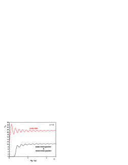
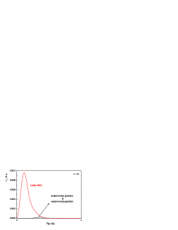
FIG. 1.: The absorption (Fig.1(a)) and emission (Fig.1(b)) spectra for the scalar- and vector-mode gravitons when $n=0$. For a comparision the spectra for the spin-$0$ field are plotted together. As Eq.(15) implies, the spectra for both gravitons are exactly identical. Fig.1(b) indicates that the emission rates for the gravitons are negligible compared to that for the spin-$0$ field when there is no extra dimension.

Fig.1 shows the total absorption and emission rates for the vector(or axial)-mode graviton and scalar(or polar)-mode graviton when $n=0$. To compare the graviton spectra with those for the low-spin field, we plot the absorption and emission rates for the spin-$0$ scalar field together. As Eq.(15) implies, the absorption and emission spectra for both graviton modes are exactly identical. As Fig.1(b) indicates, the emission rates for the gravitons are much smaller than that for the spin-$0$ field. The total emission rates for both gravitons are only $5.16\%$ of that for the spin-$0$ field. Thus, in $4d$ the Hawking radiation for the low-spin fields such as standard model fields is dominant one. However, the situation is drastically changed when the extra dimensions exist.

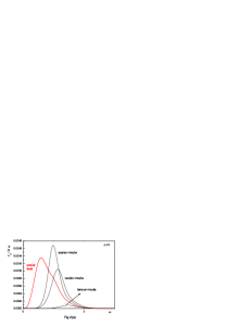
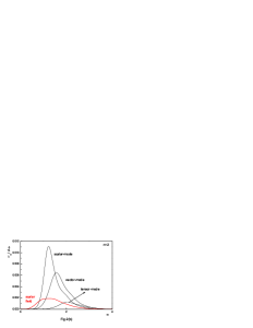
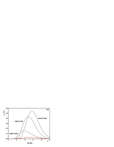
FIG. 2.: The emission spectra for the scalar-, vector- and tensor-mode gravitons when $n=1$ (Fig.2(a)), $n=2$ (Fig.2(b)) and $n=6$ (Fig.2(c)). The spectra for the spin-$0$ field are plotted together for a comparision. In general the emissivities for all fields increase with increasing $n$. However, the increasing rate for the gravitons are much larger than that for the spin-$0$ field. Thus, Hawking radiation for the gravitons becomes more and more significant when the extra dimensions exist.

Fig.2 shows that the total emission rates for the scalar-, vector-, and tensor-mode gravitons when $n=1$, $2$, and $6$. Like Fig.1 the emission spectrum of the spin-$0$ field is plotted together for a comparision. As Fig.2 indicates, the emissivities for all fields generally increase with increasing $n$. However, the increasing rates for the gravitons in the Hawking emissivities with increasing $n$ is much larger than that for the spin-$0$ field.

Table 1 shows the relative emissivities when $n=0$, $1$, $2$ and $6$. When $n=2$, the emission rate for the scalar mode graviton is almost three times than that for the spin-$0$ field. When $n=6$, the emission rate for the tensor-mode graviton is seventeen times than that for the spin-$0$ field!!! The remarkable fact is that the ratio of the tensor-mode graviton to the spin-$0$ field increases rapidly with increasing $n$ compared to other graviton modes.

In this letter we computed the absorption and emission spectra for the various modes of the bulk gravitons in the higher-dimensional non-rotating black hole background. The total emissivities for the gravitons are only $5.16\%$ compared to that for the spin-$0$ field in four dimensions. However, this ratio increases rapidly when the extra dimensions exist. When, for example, $n=1$, $2$ and $6$, this ratio goes to $147.7\%$, $595.2\%$ and $3496\%$, respectively. This fact indicates that the emission of the higher-spin field like gravitons becomes more and more dominant and has a experimental significance when there are many extra dimensions. Same conclusion was derived in the emission on the brane[14]. Thus, it is important in our opinion to re-examine the EHM argument “black holes radiate mainly on the brane” with considering the Hawking radiation for the gravitons. We hope to study this issue in the future.

Acknowledgement: This work was supported by the Kyungnam University Research Fund, 2006.

REFERENCES

• [1] J. Polchinski, String Theory (Cambridge University Press, Cambridge, 1998).
• [2] N. Arkani-Hamed, S. Dimopoulos and G. Dvali, The Hierarchy Problem and New Dimensions at a Millimeter, Phys. Lett. B429 (1998) 263 [hep-ph/9803315]; L. Antoniadis, N. Arkani-Hamed, S. Dimopoulos and G. Dvali, New Dimensions at a Millimeter to a Fermi and Superstrings at a TeV, Phys. Lett. B436 (1998) 257 [hep-ph/9804398]; L. Randall and R. Sundrum, A Large Mass Hierarchy from a Small Extra Dimension, Phys. Rev. Lett. 83 (1999) 3370 [hep-ph/9905221]; L. Randall and R. Sundrum, An Alternative to Compactification, Phys. Rev. Lett. 83 (1999) 4690 [hep-th/9906064].
• [3] S. B. Giddings and T. Thomas, High energy colliders as black hole factories: The end of short distance physics, Phys. Rev. D65 (2002) 056010 [hep-ph/0106219]; S. Dimopoulos and G. Landsberg, Black Holes at the Large Hadron Collider, Phys. Rev. Lett. 87 (2001) 161602 [hep-ph/0106295]; D. M. Eardley and S. B. Giddings, Classical black hole production in high-energy collisions, Phys. Rev. D66 (2002) 044011 [gr-qc/0201034]; D. Stojkovic, Distinguishing between the small ADD and RS black holes in accelerators, Phys. Rev. Lett. 94 (2005) 011603 [hep-ph/0409124]; V. Cardoso, E. Berti and M. Cavagliร , What we (donโ€™t) know about black hole formation in high-energy collisions, Class. Quant. Grav. 22 (2005) L61 [hep-ph/0505125].
• [4] C. M. Harris and P. Kanti, Hawking Radiation from a $(4+n)$-dimensional Black Hole: Exact Results for the Schwarzschild Phase, JHEP 0310 (2003) 014 [hep-ph/0309054]; P. kanti, Black Holes in Theories with Large Extra Dimensions: a Review, Int. J. Mod. Phys. A19 (2004) 4899 [hep-ph/0402168].
• [5] R. Emparan, G. T. Horowitz and R. C. Myers, Black Holes radiate mainly on the Brane, Phys. Rev. Lett. 85 (2000) 499 [hep-th/0003118].
• [6] E. Jung and D. K. Park, Absorption and Emission Spectra of an higher-dimensional Reissner-Nordstrรถm black hole, Nucl. Phys. B717 (2005) 272 [hep-th/0502002].
• [7] Y. B. Zelโ€™dovich, Generation of waves by a rotating body, JETP Lett. 14 (1971) 180; W. H. Press and S. A. Teukolsky, Floating Orbits, Superradiant Scattering and the Black-hole Bomb, Nature 238 (1972) 211; A. A. Starobinskii, Amplification of waves during reflection from a rotating black hole, Sov. Phys. JETP 37 (1973) 28; A. A. Starobinskii and S. M. Churilov, Amplification of electromagnetic and gravitational waves scattered by a rotating black hole, Sov. Phys. JETP 38 (1974) 1.
• [8] V. Frolov and D. Stojkoviฤ‡, Black hole radiation in the brane world and the recoil effect, Phys. Rev. D66 (2002) 084002 [hep-th/0206046]; V. Frolov and D. Stojkoviฤ‡, Black Hole as a Point Radiator and Recoil Effect on the Brane World, Phys. Rev. Lett. 89 (2002) 151302 [hep-th/0208102]; V. Frolov and D. Stojkoviฤ‡, Quantum radiation from a $5$-dimensional black hole, Phys. Rev. D67 (2003) 084004 [gr-qc/0211055]. E. Jung, S. H. Kim and D. K. Park, Condition for Superradiance in Higher-dimensional Rotating Black Holes, Phys. Lett. B615 (2005) 273 [hep-th/0503163]; E. Jung, S. H. Kim and D. K. Park, Condition for the Superradiance Modes in Higher-Dimensional Black Holes with Multiple Angular Momentum Parameters, Phys. Lett. B619 (2005) 347 [hep-th/0504139].
• [9] D. Ida, K. Oda and S. C. Park, Rotating black holes at future collider: Greybody factors for brane field, Phys. Rev. D67 (2003) 064025 [hep-th/0212108]; C. M. Harris and P. Kanti, Hawking Radiation from a $(4+n)$-Dimensional Rotating Black Hole [hep-th/0503010]; D. Ida, K. Oda and S. C. Park, Rotating black holes at future colliders II : Anisotropic scalar field emission, Phys. Rev. D71 (2005) 124039 [hep-th/0503052]; G. Duffy, C. Harris, P. Kanti and E. Winstanley, Brane decay of a $(4+n)$-dimensional rotating black hole: spin-00 particle, JHEP 0509 (2005) 049 [hep-th/0507274]; M. Casals, P. Kanti and E. Winstanley, Brane Decay of a $(4+n)$-Dimensional Rotating Black Hole II: spin-$1$ particles [hep-th/0511163].
• [10] E. Jung and D. K. Park, Bulk versus Brane in the Absorption and Emission: $5$D Rotating Black Hole Case, Nucl. Phys. B731 (2005) 171 [hep-th/0506204].
• [11] T. Regge and J. A. Wheeler, Stability of a Schwarzschild Singularity, Phys. Rev. 108 (1957) 1063.
• [12] H. Kodama and A. Ishibashi, A master equation for the gravitational perturbations of maximally symmetric black holes in higher dimensions, Prog. Theor. Phys. 110 (2003) 701 [hep-th/0305147].
• [13] A. S. Cornell, W. Naylor and M. Sasaki, Graviton emission from a higher-dimensional black hole, JHEP 0602 (2006) 012 [hep-th/0510009]; V. Cardoso, M. Cavagliร  and L. Gualtieri, Black hole particle emission in higher-dimensional spacetime, Phys. Rev. Lett. 96 (2006) 071301 [hep-th/0512002]; Hawking emission of gravitons in higher dimensions: non-rotating black hole JHEP 0602 (2006) 021; S. Creek, O.Efthimiou, P. Kanti and K. Tamvakis, Graviton Emission in the Bulk from a Higher-Dimensional Schwarzschild Black Hole [hep-th/0601126].
• [14] D. K. Park, Hawking Radiation of the Brane-Localized Graviton from the $(4+n)$-dimensional Black Hole [hep-th/0512021].
• [15] C. V. Vishveshwara, Scattering of Gravitational Radiation by a Schwarzschild Black-hole, Nature 227 (1970) 936.
• [16] F. J. Zerilli, Effective Potential for even-parity Regge-Wheeler Gravitational Perturbation Equations, Phys. Rev. Lett. 24 (1970) 737.
• [17] S. Chandrasekhar, The Mathematical Theory of Black Hole (Oxford University Press, New York, 1983).
• [18] E. Newman and R. Penrose, An Approach to Gravitational Radiation by a Method of Spin Coefficients, J. Math. Phys. 3 (1962) 566.
• [19] S. W. Hawking, Particle Creation by Black Holes, Commun. Math. Phys. 43 (1975) 199.