Abstract

We give a new, manifestly spacetime-supersymmetric method for calculating superstring scattering amplitudes, using the ghost pyramid, that is simpler than all other known methods. No pictures nor non-vertex insertions are required other than the usual $b$ and $c$ ghosts of the bosonic string. We evaluate some tree and loop amplitudes as examples.

1 Introduction

Many formalisms have been introduced for calculating scattering amplitudes for superstrings. The most practical of these have been (covariant) Ramond-Neveu-Schwarz (RNS) [1], (lightcone) Green-Schwarz (GS) [2], hybrid RNS-GS (H) [3], and pure spinor (PS) [4]. All of these have (at least) two important defects:

(1) Some kind of insertion is required. It may be separate from the vertices, or may be combined with some vertices to put them into different “pictures”. The result is to complicate the calculations or destroy manifest symmetry. (The only exception is tree graphs with external bosons only, where such methods make cyclic symmetry more obscure but avoid producing extra terms that cancel.)

(2) Supersymmetry is not completely manifest. The most serious case is RNS, where fermion vertices are much more complicated than boson (because the spinors are not free fields, so in practice noncovariant exponentials of bosons must be used), and sums over spin structures (periodic/antiperiodic boundary conditions) must be performed in loops. In the GS and H cases there is partial supersymmetry (and partial 10D Lorentz invariance), which complicates vertices for the “longitudinal” directions, which are required for general higher-point calculations; for this reason we will not consider GS and H in detail. The most symmetric is PS, which has only an integration measure that is explicitly dependent on the spinor coordinates.

In a previous paper [5] we introduced a new formalism for the superstring (based on a similar one for the superparticle [6]) using an infinite pyramid of ghosts for the spinor coordinate (GP) [7]. A derivation was also given from a covariant action. (The RNS action is not spacetime-supersymmetry covariant. The GS action [8] has defied covariant quantization [9]. The H and PS formalisms do not follow from the quantization of an action with general worldsheet metric.) The Becchi-Rouet-Stora-Tyutin operator found there was rather complicated, but fortunately none of the results of our previous paper will be needed explicitly here for calculation, but only for justification of the validity of our approach. In fact, the gauge-fixed action and massless vertex operators were guessed much earlier [10]. (An early attempt to apply them to amplitude calculations failed because spinor ghosts were not included [11].) The fact that these simple rules can be applied so naively hints that perhaps an even simpler formalism exists that implies the same rules.

There are (at least) two new conceptual results in this paper (in addition to the explicit calculations), both of which involve the treatment of zero-modes. These allow us to evaluate trees and loops without evaluating explicit integrals or (super)traces over these zero-modes, thereby solving the above two problems:

(1) In loop calculations we infrared regularize the worldsheet propagators. In principle one should do this anyway, since IR divergences are notorious in two dimensions, especially for 2D conformal field theories, but usually such problems are avoided by examining only IR-safe quantities. In our case such a regularization allows a simple counting of the infinite number of zero-modes arising from the ghost pyramid (including those from the physical spinor), with the only result being the introduction of factors of 1/4 due to the usual summation $1-2+3-...=1/4$. (Regularization of $x$ zero-modes is unnecessary; it only replaces the momentum-conservation $\delta$-function with a sharp Gaussian.)

(2) In tree graphs these zero-modes do not appear separately, having been absorbed into the definition of the (first-quantized) vacuum. Specifically, since we do not perform explicit integration over spinor zero-modes, we also do not need to define measure factors for such integrations, make insertions of operators (essentially Dirac $\delta$-functions in those modes) to kill those modes, nor use operators of different pictures to hide such insertions. We do not make special manipulations to deal with such modes; care of them is taken automatically by naively ignoring them. Although we do not analyze this vacuum (or other) state in detail here (we effectively work with the old Heisbenberg matrix mechanics, ignoring Schrödinger wave functions), we explain why such behavior is implied by the standard N=1 superspace formulation of the vector multiplet.

The net result of these ideas is that the calculational rules are the most naive generalization of the rules of the bosonic string: (1) The $b$ and $c$ ghosts appear in the same way, affecting only the measure. (2) The spinor ghosts serve only to ensure correct counting of zero-modes, and give an extra factor of 1/4 to any trace of $\gamma$-matrices. (3) IR regularization takes care of all (physical and ghost) spinor zero-modes. (4) The vertex operator for the massless states generalizes the bosonic-string one just by adding the same spin terms as in ordinary field theory or supergraphs (to include the spinor vertices), taking into account the stringy generalization of the algebra of covariant derivatives [10].

Consequently, for the case of tree graphs with external vectors only, our rules are almost identical to (R)NS calculations in the ${\cal F}_{1}$ picture. We explain the advantage of this picture and why it is more relevant to the superstring.

As an interesting side result, we show how the $\partial\theta$ terms in the $DP\Omega$ current algebra arise already in the superparticle.

2 Rules

2.1 Vertex operators

We now present the main result of this paper, the rules themselves, with examples later. (Derivations are given in the Appendices.) Here we will calculate amplitudes with only massless external states. (We also concentrate on open strings, but the results generalize in the usual way to closed.)

To a limited extent first-quantization can be applied to particles as well as to strings: It gives only one-particle irreducible graphs (vertices at the tree level), whereas for the string it gives complete S-matrix amplitudes by duality (for given loop level and external states). However, the methods are almost identical, particularly since the superparticle is the zero-modes of the superstring.

The vertex operators follow from the results of our previous paper [5] but are basically those of [10] with a small modification from ghosts (as expected from the integrated vertex operators of PS [4]):

$$V=A^{A}(x,\theta)J_{A}$$

where $A^{A}$ are superfields and $J_{A}$ are 2D currents:

$$A^{A}=(A_{\alpha},A^{a},W^{\alpha},F^{ab})$$

$$J_{A}=(\Omega^{\alpha},P_{a},D_{\alpha},\hat{S}_{ab})$$

where $J_{A}$ have zero-modes $j_{A}$, of which only $p_{a}$ and $d_{\alpha}$ act nontrivially on $A^{A}$. $D,P,\Omega$ are the currents of [10], while $\hat{S}$ is the Lorentz current of the $\theta$ ghosts (“superspin”). (Appendix A gives the relation of vertex operators between Lagrangian and Hamiltonian formalisms.)

As for the bosonic string, the integrated vertex operator is $\int V$ and the unintegrated one is $cV$; the $b$ and $c$ ghosts work in exactly the same way, to keep the measure conformal. (We could also add a term $\alpha^{\prime}(\partial_{a}A^{a})\partial c$ to the unintegrated vertex operator to avoid having to apply $\partial_{a}A^{a}=0$ [12].)

The external-state superfields and the currents can be expanded in $\theta$ for evaluation in terms of 2D Green functions of the fundamental variables: For example, the vertex for just the vector is then

$$V_{B}=A_{a}(x)\partial x^{a}+{\textstyle{1\over 2}}F^{ab}(x)S_{ba}$$

where $S$ is the Lorentz current of all $\theta$’s, physical and ghost. There are also terms higher-order in $\theta$, but in the absence of external fermions there are no $\pi$’s to cancel the extra $\theta$’s, so such terms won’t contribute. Because of its universality, this form is useful for comparison to other formalisms.

2.2 Current algebra

However, when calculating general amplitudes (including fermions), it is more convenient to expand neither the currents nor superfields (thus manifesting supersymmetry). This requires rules for evaluating products of arbitrary numbers of currents. Although this problem is generally intractable for arbitrary representations of arbitrary current algebras, in our case it is relatively simple:

(1) $\hat{S}$ doesn’t act on the superfields. It is quadratic in free fields, so the matrix element of any product of such currents is simply the sum of products of loops of them (in 2D perturbation theory), from contracting the (ghost) $\theta$ of one with the $\pi$ of the next. Each such loop contributes the trace of the product of the $\gamma$ matrices that appear sandwiched between $\theta$ and $\pi$ in $\hat{S}_{ab}=\theta\gamma_{ab}\pi|_{>}$ (where “$|_{>}$” means to restrict to ghosts).

(2) The remaining currents $D_{\alpha}$, $P_{a}$, and $\Omega^{\alpha}$ form a separate algebra. Although their “loops” are more complicated (since $D$ is cubic in free fields), the structure constants are so simple that no loop contains more than 4 currents: only the combinations $PP$, $D\Omega$, $DDP$, or $DDDD$. Since $D$ and $P$ (but not $\Omega$) can also act on superfields, the matrix element of such currents and superfields reduces to the sum of products of these 4 types with strings of $D$ and $P$ acting on superfields.

The loops are:

$$\langle P_{a}(1)P_{b}(2)\rangle = -\eta_{ab}G_{x}^{\prime\prime}(1,2)$$

$$\langle D_{\alpha}(1)\Omega^{\beta}(2)\rangle = -i\delta_{\alpha}^{\beta}G_{\theta}^{\prime}(1,2)$$

$$\langle D_{\alpha}(1)D_{\beta}(2)P_{a}(3)\rangle = -i\gamma_{a\alpha\beta}[2G_{\theta}(2,3)G_{\theta}^{\prime}(1,3)-2G_{\theta}(1,3)G_{\theta}^{\prime}(3,2)$$

$$+G_{\theta}(1,2)(G_{x}^{\prime\prime}(1,3)+G_{x}^{\prime\prime}(2,3))]$$

$$\langle D_{\alpha}(1)D_{\beta}(2)D_{\gamma}(3)D_{\delta}(4)\rangle = 2iG_{\theta}^{\prime}(1,2)G_{\theta}(1,3)G_{\theta}(1,4)(\gamma^{a}_{\alpha\gamma}\gamma_{a\delta\beta}-\gamma^{a}_{\alpha\delta}\gamma_{\gamma\beta})$$ (2.2.1)

$$+2iG_{\theta}^{\prime}(1,2)G_{\theta}(2,3)G_{\theta}(2,4)(\gamma^{a}_{\beta\delta}\gamma_{\gamma\alpha}-\gamma^{a}_{\beta\gamma}\gamma_{a\delta\alpha})$$

$$+iG_{x}^{\prime\prime}(1,2)\left[G_{\theta}(1,3)G_{\theta}(2,4)\gamma^{a}_{\alpha\gamma}\gamma_{a\beta\delta}\right.$$

$$\left.~{}~{}-G_{\theta}(2,3)G_{\theta}(1,4)\gamma^{a}_{\beta\gamma}\gamma_{a\alpha\delta}\right]+\mbox{perm.}$$

where $\langle\quad\rangle$ refers to fully contracted operator products, and “1” means “$z_{1}$”, etc. We have distinguished the $x$ and $\theta\pi$ Green functions ($G_{x}$ and $G_{\theta}$) because only $G_{\theta}$ gives zero-mode corrections, which is explained in detail in Appendix E. For N string loops, $G$ is a genus-N Green function: for trees, $G_{x}^{\prime}(z_{1}-z_{2})=-iG_{\theta}(z_{1}-z_{2})=-\frac{1}{z_{1}-z_{2}}$ and $G_{x}^{\prime\prime}(z_{1}-z_{2})=-iG_{\theta}^{\prime}(z_{1}-z_{2})=\frac{1}{(z_{1}-z_{2})^{2}}$; at 1 string loop they are Jacobi theta functions and their derivatives; etc.

The action of the currents on the fields is given by considering all possible symmetrizations of the $D$’s. Any symmetrization of 2 $D$’s (acting on a field) gives

$$D_{(\alpha}(1)D_{\beta)}(2)\quad\to\quad G_{\theta}(1,2)\gamma^{a}_{\alpha\beta}[P_{a}(1)+P_{a}(2)]$$ (2.2.2)

This reduces any string of currents to sums of strings of $P$’s times antisymmetrized strings of $D$’s, which are evaluated as

$$D_{[\alpha}(1)\cdots D_{\beta]}(2)P_{a}(3)\cdots P_{b}(4)A(5)=G_{\theta}(1,5)\cdots G_{x}^{\prime}(4,5)(d_{[\alpha}\cdots d_{\beta]}p_{a}\cdots p_{b}A)(5)$$ (2.2.3)

where $p_{a}=-i\partial_{a}$, and we can replace $\pi_{\alpha}=\partial/\partial\theta^{\alpha}$ with the usual supersymmetry covariant derivative $d_{\alpha}$ in such antisymmetrizations since final results can always be evaluated at $\theta=0$ by supersymmetry.

By 10D dimensional analysis, any $\hat{S}$ loop is dimensionless, while any $DP\Omega$ loop has dimension 2. This implies (contrary to expectations, but well known from the bosonic case) that each $DP\Omega$ loop carries an extra factor of the inverse of $\alpha^{\prime}$. (In the particle case, there is instead an inverse of $z$.) Thus, the maximum number of $DP\Omega$ loops gives the lowest power in momenta, and each loop less gives two more powers of momenta. (One way to see the dimensional analysis is to note that each current acting on a superfield gives a $G_{x}^{\prime}$ or $G_{\theta}$. The same is true in a $DP\Omega$ loop, except that 2 currents “close” the loop to give a $G_{x}^{\prime\prime}$ or $G_{\theta}^{\prime}$. Thus, each $DP\Omega$ loop introduces an extra factor of $G_{x}^{\prime\prime}(\mbox{or}~{}G_{\theta}^{\prime})/(G_{\theta})^{2}$. On the other hand, closing an $\hat{S}$ loop gives a $(G_{\theta})^{2}$ instead of $G_{\theta}^{\prime}$, so such loops give no extra factor.)

Finally, there is the usual momentum dependence coming from Green functions connecting the superfields to each other, from their $x$ dependence only: For the usual plane waves,

$$\langle A(1)\cdots A(N)\rangle=A\cdots A\ e^{-\sum_{i<j}k_{i}\cdot k_{j}G_{x}(i,j)}$$ (2.2.4)

with units $\alpha^{\prime}=1/2$ for the string.

2.3 Component expansion

The final result for an amplitude is given as a “kinematic factor” times a scalar function of momentum invariants, expressed as an integral over the worldsheet positions of the vertices. The kinematic factor is expressed, by the above procedure, as a sum of products of superfields, representing external state wave functions. The string rules have effectively already performed covariant $\theta$ integration, so these superfields may be evaluated at $\theta=0$. (As in the usual superspace methods, where $\theta$ expansion and integration is replaced by the action on the “Lagrangian” of the product of all supersymmetry covariant derivatives $d_{\alpha}$, supersymmetry guarantees that all $\theta$ dependence cancels, up to total $x$ derivatives.)

The evaluation of spinor derivatives follows from the (linearized) constraints on the gauge covariant superspace derivatives, and their Bianchi identities [13]. The result is

$$d_{(\alpha}A_{\beta)} = 2\gamma^{a}_{\alpha\beta}A_{a}$$

$$d_{\alpha}A_{a}-\partial_{a}A_{\alpha} = 2\gamma_{a\alpha\beta}W^{\beta}$$

$$d_{\alpha}W^{\beta} = {\textstyle{1\over 2}}\gamma^{ab}{}_{\alpha}{}^{\beta}F_{ba}$$

$$d_{\alpha}F^{ab} = 2i\gamma^{[a}_{\alpha\beta}\partial^{b]}W^{\beta}$$ (2.3.1)

The result is also (linearized) gauge invariant (except for $\partial_{a}A^{a}=0$, as explained above), so one may use a Wess-Zumino gauge where $A_{\alpha}=0$ at $\theta=0$. (A review of gauge covariant derivatives appears in Appendix C.)

2.4 IR regularization

In evaluation of tree graphs there is the usual $\delta$-function for conservation of total momentum from the zero-modes of $x$, but $\theta$ effectively has no zero-modes: The effect of the $\theta$ ghosts is to mimic GS where, unlike momentum, the 8 surviving fermionic variables of the lightcone are self-conjugate, and thus have no vanishing eigenvalues. Thus there is no residual integration over $\theta$ zero-modes (unlike PS).

In loops there is the usual summation over $\theta$ zero-modes in the sum over all states, but the ghosts again mimic GS by effectively reducing the number to 8 from the physical 32 ($\theta$ and conjugate $\pi$), using the sum

$$1-2+3-4+...=1/4$$

when counting the number of $\theta$’s at successive ghost levels (alternating in statistics). Application of this rule requires infrared regularization of the 2D Green functions to “remove” the zero-modes: The factor in the partition function from these zero-modes is the IR regulator $\epsilon$ to the power $16\times 1/4=4$ (from the 16-valued spinor index on the $\theta$’s). Since the $\theta\pi$ Green function goes as $1/\epsilon$ (+ the usual finite expression + ${\cal O}(\epsilon)$), the amplitude vanishes until 4-point. Thus the power of the regulator counts zero-modes.

The 1/4 rule also applies in $\gamma$-matrix algebra. Amplitudes involve traces of products of $\gamma$-matrices. These matrices are the same at each ghost level (except that chirality, as well as statistics, alternates with ghost level), so the net effect of the ghosts appears only when taking a trace: Applying the usual $\gamma$-matrix identities, the trace is reduced to $str(I)=16\times 1/4=4$, again reproducing GS. The difference from GS is that the $\gamma$-matrices are for 10 dimensions, so the result is Lorentz covariant, and the usual 10D Levi-Civita tensor is produced (where appropriate) instead of spurious 8D $\epsilon$-tensors. For example, anomalies can be found from 6-point graphs. (Details of the regularized Green functions are given in Appendix E.)

3 Trees

3.1 RNS pictures

We begin by proving that the trees with external bosons are identical to those obtained from (the NS sector of) RNS. This is most obvious in the ${\cal F}_{1}$ picture. Although this picture was the original one to be used in (R)NS amplitude calculations, it was immediately replaced with the ${\cal F}_{2}$ picture [14]. We refer here to the picture for the physical coordinates ($x,\psi$), and not just the ghosts: For example, vector vertices have always been $\partial x+...$ except for two $\psi$ vertices, while in the ${\cal F}_{1}$ picture all vertices are $\partial x+...$ . In the proof of equivalence [14], starting from the ${\cal F}_{1}$ picture, one pulls factors of (the $\pm 1/2$ modes of) $G=\psi\cdot\partial x$ (worldsheet supersymmetry generator) off of two unintegrated $\partial x+...$ vertices to turn them into $\psi$ vertices, then collides the $G$’s to produce (the 0 mode of) a worldsheet energy-momentum tensor $T$, which gives a constant acting on a physical state. (With ghosts the approach is similar, with $G$ replaced with the picture-changing operator, which is simply the operator product of the gauge-fixed $G$ with $e^{\phi}$ in terms of the bosonized ghost $\phi$.) The resulting rules are then the same as the rules for the bosonic string, including the factors of $c$ for the three unintegrated vertices, except that the $\partial x$ vertex has the extra spin term. The $\beta$ and $\gamma$ ghosts are completely ignored; the vacuum used is in what is usually called the “$-1$ picture”, so the zero-modes of $\gamma$ (or $\phi$) are already eliminated. (What is usually called “picture changing” in the modern covariant formalism would start with the ${\cal F}_{2}$ picture, introduce two factors of picture changing times inverse picture changing, use the picture changing to change the two $\psi$ vertices, and use the inverses to change the initial and final vacuua. Unfortunately, the inverse has an overall factor of $c$, so in the new vacuum $\langle\gamma\gamma c\rangle\sim 1$ [15], and the $\gamma$’s pick out the $\psi$ terms again in two of the unintegrated vertices $\gamma\psi+c(\partial x+...)$. Thus such transformations preserve the ${\cal F}_{2}$ picture as far as the physical sector is concerned.)

Historically, the ${\cal F}_{1}$ picture was introduced first because: (1) It is more similar to the bosonic string, and (2) cyclic symmetry is manifest (no need to bother with picture changing). The ${\cal F}_{2}$ picture was then chosen because the physical-state conditions were more obvious. Although in modern language the BRST conditions are clear in either picture, it’s interesting to examine the differences in the pictures if the ghosts are ignored, since the ghosts differ in different formulations of the superstring, but all formulations have similar integrated vertices. Then the ground state of the ${\cal F}_{2}$ picture is the “physical” tachyon, at $m^{2}=-1/2$, while in the ${\cal F}_{1}$ picture it’s an “unphysical” tachyon at $m^{2}=-1$. Furthermore, the ${\cal F}_{1}$ picture has an additional “ancestor” trajectory 1/2 unit higher than the leading physical trajectory. These “disadvantages” were noticed in the days before Gliozzi-Scherk-Olive projection. On the other hand, for the superstring this projection eliminates the “physical” tachyon as well as the ancestor trajectory. So the only remaining additional unphysical state of the ${\cal F}_{1}$ picture is its vacuum, while GSO projection has eliminated the vacuum of the ${\cal F}_{2}$ picture altogether! This suggests that any comparison of the RNS formulation to others would be easier in the ${\cal F}_{1}$ picture.

3.2 For bosons only

The proof of equivalence of the ${\cal F}_{1}$ vector trees to the vector trees of our formalism is then simple: One only has to note that the operator algebra of the vertices is identical. But the vertices are identical in form; only the explicit representation of the spin current is different. So one only has to check the equivalence of the two current algebras. Since they are both (10D) Lorentz currents, quadratic in free fields, this means just checking that the central charge is the same. (The same method has been used for comparing PS to the ${\cal F}_{2}$ picture [16].) The reason the result for the central charge is the same is that the GP result is the same as the GS result: The $\gamma$-matrix algebra is the same except for a trace, which is 1/4 as big in the lightcone as for a covariant spinor, but GP again gets a factor of 1/4 from summing over ghosts. (As we’ll see below, similar arguments apply in loops, unless one gathers enough spin currents to produce a Levi-Civita tensor.)

The calculations in the ${\cal F}_{1}$ picture (and GP) are somewhat harder than the ${\cal F}_{2}$ picture because two vertices have been replaced with ones that generate more terms, which cancel. Also, RNS bosonic trees are simpler than PS or GP because integration over the vector fermion $\psi^{a}$ effectively does all $\gamma$-matrix algebra. However, tree amplitudes with fermions are much harder in RNS than PS or GP (and increase in difficulty as the number of fermions increases). PS is still simpler than GP, because $\theta$ integration takes the place of the change in the two vertices, and so also avoids generating extra terms. So, for trees RNS is the easiest for pure bosons, PS is easiest with fermions, and GP is a bit harder than both. However, GP requires fewer rules, since all vertices are the same, so it produces more terms at an intermediate stage but is easier to “program”. This feature is a peculiarity of tree graphs: At the loop level we’ll see that GP maintains the simplest rules, while RNS produces extra terms that cancel (because supersymmetry is not manifest).

At first sight these rules for GP might seem peculiar because there is no explicit integral over spinor zero-modes, as expected in known superspace approaches. The answer can be seen from examining the simpler (and better understood) case of 4D N=1 super Yang-Mills. Since the vacuum of the open bosonic string can be identified with a constant Yang-Mills ghost (or gauge parameter), we examine the ghost superfield $\phi$, and look at $\phi=1$, a supersymmetric condition. Since this superfield is chiral, and supergraphs prefer unconstrained superfields, we write $\phi=\bar{d}^{2}\chi$ in terms of a general complex superfield $\chi$. Then clearly $\chi=\bar{\theta}^{2}$ in our case. This is still supersymmetric because of the gauge invariance $\delta\chi=\bar{d}_{\dot{\alpha}}\lambda^{\dot{\alpha}}$. Furthermore, this $\chi$ has a nice norm, $\int d^{4}\theta\ |\chi|^{2}=1$. In Hilbert-space notation we thus write the norm and supersymmetry as

$$\langle 0|0\rangle=1,\quad\quad q_{\alpha}|0\rangle=Q|\lambda\rangle_{\alpha}$$

so the vacuum is supersymmetry invariant up to a BRST triviality, and the norm includes zero-mode integration, but the extra zero-modes are absorbed by the vacuua, and no insertions are required. (We could also use $|\lambda\rangle_{\alpha}=\Lambda_{\alpha}|0\rangle$ to define $\hat{q}_{\alpha}=q_{\alpha}-[Q,\Lambda_{\alpha}]$, $\hat{q}_{\alpha}|0\rangle=0$.) This supersymmetry of the vacuum is enough to ensure the amplitudes transform correctly, since the vertex operators are superfields times supersymmetry invariant currents, and the vacuum and vertex operators (integrated and unintegrated) are BRST invariant. (The unintegrated vertex operators we have used are BRST invariant only after including terms higher-order in ghost $\theta$’s, which don’t contribute to amplitudes for massless external states, and probably not for massive ones either, because of the absence of ghost $\pi$’s to cancel them.) The fact that the vacuum is “half-way” up in the $\theta$ expansion was also found for the expansion in the spinor ghost coordinates in a lightcone analysis of the BRST cohomology for the GP superparticle [6]. Note that this choice of vacuum is relevant only for trees; at 1 loop one effectively does a (super)trace over all states rather than a vacuum expectation value, so the vacuum is irrelevant. (We assume a similar situation will occur at higher loops, but we have not checked yet.) As we will see below, one important affect on this vacuum choice for trees, which does not affect loops, is that:

For tree graphs only, background fields are always evaluated in the Wess-Zumino gauge.

If this vacuum structure can be better understood, it might be possible to find an analog of the ${\cal F}_{2}$ picture for GP, avoiding the production of extra canceling terms, making it the simplest formalism even for trees. As an attempt at formulating such a picture, one can consider this picture for RNS: For pure bosons, two vertices must be in the “$-1$ picture”, so it is convenient to consider those two as the initial and final states, using the vertex operators on the initial and final vacuua. Generalizing only those 2 states to include fermions, we can write their vertex operators as in GP, but now identifying the currents with

$$D_{\alpha}=e^{-\phi/2}S_{\alpha},\quad P_{a}=e^{-\phi}\psi_{a},\quad\Omega^{\alpha}=e^{-3\phi/2}S^{\alpha}$$

The first two are the usual for the spinor (in the $-1/2$ picture) and vector (in the $-1$ picture), while the last can be identified as that for the spinor in the $-3/2$ picture (also with conformal weight 1) if we use the “supersymmetric gauge”

$$W^{\alpha}\sim\gamma^{a\alpha\beta}\partial_{a}A_{\beta}$$

instead of the WZ gauge. (Hitting $cA_{\alpha}\Omega^{\alpha}$ with picture changing produces $cW^{\alpha}D_{\alpha}$.) These currents satisfy almost the same algebra as the usual ones (including $DP\sim\Omega$, to leading order); the only exceptions are $\Omega P$ and $\Omega\Omega$. As a guess for the GP analog, we can then try to construct a new $DP\Omega$ for this picture that depends only on the ghosts. Unfortunately (the simplest guess for) this construction seems not to work, apparently because the dependence on the WZ gauge hasn’t been eliminated, and is incompatible with the supersymmetric gauge.

3.3 General 3-point

As explained in Section 2, we prefer the superfield formalism for the calculation of amplitudes with fermions. This includes the all-vector amplitude in the same calculation. The only nonvanishing operator products for the 3-point tree, after applying the Landau gauge condition ($\partial\cdot A=0$), are:

$$A.\quad\langle P_{a}(1)P_{b}(2)\rangle\times P_{c}(3)A^{a}(1)A^{b}(2)A^{c}(3)+\mbox{permutations}$$

$$B.\quad(P_{c}(3)A^{a}(1))(P_{a}(1)A^{b}(2))(P_{b}(2)A^{c}(3))+\mbox{perm.}$$

$$C.\quad\langle P_{a}(1)P_{b}(2)\rangle\times D_{\alpha}(3)A^{a}(1)A^{b}(2)W^{\alpha}(3)+\mbox{perm.}$$

$$D.\quad\langle D_{\alpha}(1)D_{\beta}(2)P_{a}(3)\rangle\times W^{\alpha}(1)W^{\beta}(2)A^{a}(3)+\mbox{perm.}$$

$$E.\quad\langle D_{\beta}(2)\Omega^{\gamma}(3)\rangle\times D_{\alpha}(1)W^{\alpha}(1)W^{\beta}(2)A_{\gamma}(3)+\mbox{perm.}$$

$$F.\quad(D_{\gamma}(3)W^{\alpha}(1))(D_{\alpha}(1)W^{\beta}(2))(D_{\beta}(2)W^{\gamma}(3))+\mbox{perm.}$$

$$G.\quad\langle\hat{S}_{ab}(1)\hat{S}_{cd}(2)\rangle\times P_{e}(3)F^{ab}(1)F^{cd}(2)A^{e}(3)+\mbox{perm.}$$

$$H.\quad\langle\hat{S}_{ab}(1)\hat{S}_{cd}(2)\hat{S}_{ef}(3)\rangle\times F^{ab}(1)F^{cd}(2)F^{ef}(3)$$ (3.3.1)

where the $\hat{S}$ contraction is the usual $\gamma$ trace.

The other contributions, like $(\langle D_{\alpha}\Omega^{\beta}\rangle P)\cdot AW^{\alpha}A_{\beta},~{}~{}(\langle SS\rangle D_{\alpha})\cdot FFW^{\alpha},~{}~{}(PPD_{\alpha})\cdot AAW^{\alpha}$ and $(PD_{\alpha}D_{\beta})AWW$, all vanish using $k_{i}\cdot k_{j}=0,\mathchoice{k\kern-5.52084pt{\hbox to5.52084pt{\hfil$\displaystyle{/}$\hfil}}}{k\kern-5.52084pt{\hbox to5.52084pt{\hfil$\textstyle{/}$\hfil}}}{k\kern-3.86458pt{\hbox to3.86458pt{\hfil$\scriptstyle{/}$\hfil}}}{k\kern-2.7604pt{\hbox to2.7604pt{\hfil$\scriptscriptstyle{/}$\hfil}}}W=0$ in the Wess-Zumino gauge. We give some details of the calculation in Appendix F.

Notice that F and H combine to give the GP sum $1-2+3-4\cdots=1/4$. From these combinations we find the manifestly supersymmetric 3-point tree amplitudes for vectors and spinors

$$A^{tree}_{3} = k_{1}\cdot A(3)A(1)\cdot A(2)+k_{3}\cdot A(2)A(1)\cdot A(3)+k_{2}\cdot A(1)A(2)\cdot A(3)$$

$$+iA(1)\cdot W(2)\gamma W(3)+iA(2)\cdot W(3)\gamma W(1)+iA(3)\cdot W(1)\gamma W(2)$$

where $A(i)$ are the vectors and $W(i)$ the spinors. (Note that we use the usual anticommuting fields for the spinors; numerical evaluation involves fermionic functional differentiation, replacing these fields with the usual commuting wave functions, and may introduce signs if not all terms have the same ordering.)

This result applies to both the superparticle and superstring. In the string case there is also a factor of $1/(z_{1}-z_{2})(z_{2}-z_{3})(z_{1}-z_{3})$ from the Green functions, but this is canceled as usual with the inverse factor from the conformal measure obtained from $\langle c(1)c(2)c(3)\rangle$.

4 IR regularization

4.1 Zero modes

The kinematic factor in supersymmetric amplitudes is closely related to the spinor zero-mode problem, which is the most important problem in the Lorentz covariant superparticle and superstring. If we naively integrate over zero-modes of the infinite pyramid of spinors with no vertex attached, we find $0\cdot\infty^{2}\cdot 0^{3}\cdot\infty^{4}\cdot 0^{5}\cdot\infty^{6}\cdots$. So we need to regularize the zero-mode integration. In Appendix E we derive the 2D Green function with a 2D regularization mass, but it turns out that the zero-mode behavior of the 2D Green function is exactly that of the 1D one. So we will concentrate on the 1D case here. To do this IR regularization we introduce small mass terms in the superparticle free action (for 1D “proper time” coordinate $z$)

$$X^{a}(-\partial^{2}_{z}+\xi^{2})X_{a},\quad\quad-i\pi(\partial_{z}+\epsilon)\theta$$ (4.1.1)

Now we can fix the measure of zero-modes for $X$ and $\theta$ without ambiguity. For $X$, neglecting the Laplacian term, which vanishes for zero-modes,

$$\lim_{\xi\rightarrow 0}\int d^{D}X_{0}\ e^{-T\xi^{2}X^{2}_{0}/2-i(\sum k)\cdot X_{0}} = \lim_{\xi\rightarrow 0}\left(\frac{2\pi}{T\xi^{2}}\right)^{D/2}e^{-(\sum k)^{2}/2T\xi^{2}}$$

$$= (2\pi)^{D}\delta^{D}\left(\sum k\right)$$

$$= \int d^{D}X_{0}\ e^{-i(\sum k)\cdot X_{0}}$$

where $T$ is the range of $z$ (at 1 loop, the period). Here we used $\lim_{\xi\rightarrow 0}e^{-x^{2}/2\xi^{2}}/\sqrt{\xi}=\sqrt{2\pi}\delta(x)$. Therefore our zero-mode measure for $X$ is

$$\int dX_{0}=\lim_{\xi\rightarrow 0}\left(\frac{2\pi}{T\xi^{2}}\right)^{D/2}$$ (4.1.2)

However, this bosonic zero-mode does not appear explicitly, since this always gives momentum conservation thanks to the vertex operators.

Similarly for $\theta$ we see

$$\int d\theta\ d\pi~{}e^{iT\epsilon\pi\theta}=(i\epsilon T)^{\pm 2^{(D-2)/2}}$$ (4.1.3)

where “$\pm$” stands for fermionic and bosonic spinor respectively. Then our zero-mode measure for a spinor is

$$\int d\theta\ d\pi=\lim_{\epsilon\rightarrow 0}(i\epsilon T)^{\pm 2^{(D-2)/2}}$$ (4.1.4)

In our case we have an infinite pyramid of spinors and hence we get

$$\int d\theta\ d\pi = \lim_{\epsilon\rightarrow 0}(i\epsilon T)^{(2^{(D-2)/2})(1-2+3-4+\cdots)}$$ (4.1.5)

$$= \lim_{\epsilon\rightarrow 0}(i\epsilon T)^{2^{(D-6)/2}}$$

where we used coherent-state regularization for the ambiguous sum $1-2+\cdots=1/4$:

$$tr[(N+1)(-1)^{N}] = \int\frac{d^{2}z}{\pi}e^{-z^{*}z}\langle z|(a^{{\dagger}}a+1)(-1)^{a^{{\dagger}}a}|z\rangle$$ (4.1.6)

$$= \int\frac{d^{2}z}{\pi}e^{-|z|^{2}}(\langle z|a^{{\dagger}}a|-z\rangle+\langle z|-z\rangle)$$

$$= \int\frac{d^{2}z}{\pi}(-|z|^{2}+1)e^{-2|z|^{2}}$$

$$= -{\textstyle{1\over 4}}+{\textstyle{1\over 2}}={\textstyle{1\over 4}}$$

More intuitively

$$\frac{1}{1+x} = 1-x+x^{2}-x^{3}+x^{4}\cdots$$

$$\frac{1}{(1+x)^{2}} = 1-2x+3x^{3}-4x^{4}+\cdots$$

so at $x=1$ we get 1/2 and 1/4 respectively.

Therefore in $D=10$ we get effectively $\epsilon^{4}$ for zero-modes. So our complete spinor measure with non-zero modes is

$$\mathcal{D}\theta\ \mathcal{D}\pi\ (iT\epsilon)^{4}$$ (4.1.7)

The significant role of this effective power will be clear after we discuss the Green function.

The regularization $1-2+3-4+\cdots=1/4$ explains how we can get a physical $SO(8)$ spinor contribution out of 2 covariant 16-component spinors $\pi$ and $\theta$. Because we cannot project covariant spinors into physical spinors in a covariant way, we need to add infinitely many ghosts to achieve this 1/4 reduction in amplitudes.

4.2 Regularized Green functions

We summarize the results of Appendix E here. We find the regularized 1D Green functions for $x$ and $\theta$

$$G^{x}(z) = \frac{1}{2\xi}\frac{\cosh[\xi(|z|-T/2)]}{\sinh(\xi T/2)}$$

$$G^{\theta}(z) = i(-\partial_{z}+\epsilon)\left[\frac{1}{2\epsilon}\frac{\cosh[\epsilon(|z|-T/2)]}{\sinh(\epsilon T/2)}\right]$$ (4.2.1)

The $\epsilon$ correction to $\partial_{z}$ in $G^{\theta}$ is nontrivial because it multiplies a Green function with a $1/\epsilon$ term.

It is convenient to expand the Green functions in $\epsilon$ when we calculate scattering amplitudes:

$$G^{x} = \frac{1}{\xi^{2}T}+\sum_{n=0}^{\infty}G^{x}_{n}\xi^{n}$$

$$G^{\theta} = \frac{i}{\epsilon T}+\sum_{n=0}^{\infty}G^{\theta}_{n}\epsilon^{n}$$ (4.2.2)

where

$$G^{x}_{0} = {T\over 12}+{|z|(|z|-T)\over 2T}={T\over 12}+G^{x}_{un}$$

$$G^{\theta}_{0} = \frac{i}{2}Sign(z)-i\frac{z}{T}=G^{\theta}_{un}$$ (4.2.3)

and $G^{x}_{un}$ and $G^{\theta}_{un}$ are the usual $1D$ Green functions with periodic boundary conditions, normalized to $G_{un}(0)=0$. The extra constant will not contribute to massless amplitudes because of derivatives and $k^{2}=0$.

Because the mass (re)moves zero-modes, the usual fudges of the massless Green functions are eliminated: There is no freedom to add constants (dependent on $T$, but not $z$) to $G$, and the $\delta$ function in its equation of motion is not modified to $\delta(z)-1/T$ to preserve “charge conservation”. But the latter property is restored upon expansion in the regulator:

$$G^{x} = \frac{1}{\xi^{2}T}+\Delta G^{x},\quad(-\partial^{2}+\xi^{2})G^{x}=\delta\quad\Rightarrow\quad(-\partial^{2}+\xi^{2})\Delta G^{x}=\delta-{1\over T}$$

$$G^{\theta} = \frac{i}{\epsilon T}+\Delta G^{\theta},\quad-i(\partial+\epsilon)G^{\theta}=\delta\quad\Rightarrow\quad-i(\partial+\epsilon)\Delta G^{\theta}=\delta-{1\over T}$$ (4.2.4)

Similarly we will do this expansion for superstring Green functions. The details are given in Appendix E. However, expansion of $G^{x}$ is unnecessary, because in vertex operators $X$ appears only as $\dot{X}$ (and as an argument of the superfields), and any contraction involving this vertex operator is always finite. (The derivative kills the potentially divergent $1/\xi^{2}$ term.) For this reason $X$ regularization gives only energy-momentum conservation and is irrelevant to amplitude corrections. But $\epsilon$ expansion of $G^{\theta}$ is crucial, as we will see in the next section.

5 Loops

5.1 N$<$4 super

Here we give simple examples. The only differences from standard first-quantization of a loop of a scalar particle or bosonic string can be associated with “kinematic factors” that may also depend on the positions of the vertices on the worldline/sheet. (For a summary of the standard analysis of the other factors, see Appendix D.)

Collecting the results of the zero-mode measure and the Green function zero-mode behavior, the amplitude is zeroth order in $\epsilon$.

Since there is an $\epsilon^{4}$ in the measure, we should pick up an $\epsilon^{-4}$ in the integrand of the path integral. For example, one sub-diagram of the N-point 1-loop amplitude is proportional to

$$\oint d\epsilon~{}\epsilon^{3}~{}G^{\theta}(1,2)G^{\theta}(2,3)\cdots G^{\theta}(N,1)$$ (5.1.1)

Then to evaluate this amplitude we should expand each $G^{\theta}$ and collect terms with $\epsilon^{-4}$.

We now notice that every $G^{\theta}$ gives $i/\epsilon T$. For $N<4$ there are not enough powers of $\epsilon^{-1}$ and so their amplitudes just vanish.

There is no zero-mode behavior for any contraction involving $\partial X$ because of the derivative. Therefore $P$ contractions start to contribute only at $N=5$ (a black dot in Fig. 1).

Figure 1: Schematic diagrams for various contractions

5.2 N=4 vector only

The first nonvanishing amplitude is at $N=4$. However, this is just the case where every $G^{\theta}$ from the $S_{ab}$’s contributes $i/\epsilon T$. So the integration is trivially done for $K_{4}$ and only its spin algebra matters. There are two kinds of diagrams: the case where all 4 points are connected, and the case where each pair of points is connected separately (Fig. 1). These two diagrams have opposite sign. Each closed contraction should be traced over all ghost pyramid spinors to give $1-2+3-4+\cdots=1/4$. Therefore we get for $K_{4}$, omitting external field factors,

$$K_{4} = -\frac{1}{4}\left[tr(\gamma^{ab}\gamma^{cd}\gamma^{ef}\gamma^{gh})+\mbox{5 permutations}~{}\right]$$ (5.2.1)

$$+\frac{1}{16}\left[tr(\gamma^{ab}\gamma^{cd})tr(\gamma^{ef}\gamma^{gh})+\mbox{2 permutations}~{}\right]$$

Using the Mathematica code Tracer.m we evaluate this gamma-matrix trace to find

$$K_{4} = ~{}~{}{\textstyle{1\over 2}}(\delta^{bc}\delta^{de}\delta^{fg}\delta^{ha}+\delta^{be}\delta^{cf}\delta^{dg}\delta^{ha}+\delta^{ae}\delta^{fg}\delta^{ch}\delta^{bd}~{}+45~{}\mbox{terms}$$ (5.2.2)

$$\quad\mbox{from antisymmetrizing each pair of indices}~{}~{}[ab][cd][ef][gh])$$

$$-{\textstyle{1\over 2}}\left[(\delta^{ac}\delta^{bd}-\delta^{ad}\delta^{bc})(\delta^{eg}\delta^{fh}-\delta^{eh}\delta^{fg})\right.$$

$$\quad\quad+(\delta^{ae}\delta^{bf}-\delta^{af}\delta^{be})(\delta^{cg}\delta^{dh}-\delta^{ch}\delta^{dg})$$

$$\quad\quad+\left.(\delta^{ag}\delta^{bh}-\delta^{ah}\delta^{bg})(\delta^{ce}\delta^{df}-\delta^{cf}\delta^{de})\right]$$

This is the well-known kinematic factor for both tree and 1-loop. We can also express this results in terms of $F$ as [17]

$$F^{ac}(1)F^{b}{}_{c}(2)F_{a}{}^{d}(3)F_{bd}(4)-\frac{1}{8}F^{ab}(1)F_{ab}(2)F^{cd}(3)F_{cd}(4)$$

$$-\frac{1}{4}F^{ab}(1)F^{cd}(2)[F_{ab}(3)F_{cd}(4)-2F_{ac}(3)F_{bd}(4)]$$ (5.2.3)

which can be interpreted as “graviton”, “dilaton”, and “axion” as far as Lorentz (and not gauge) structure is concerned. (In the nonplanar case, it actually corresponds to those poles for color singlets in the 1+2=3+4 channel.)

5.3 N=4 super

Here we again prefer the superfield formalism as explained in Section 2. However, the 4-point one-loop case is dramatically simplified due to the IR regularization. Consider the 4 types of fully contracted operators again and then notice that they can have only limited $1/\epsilon$ factors, since each $G^{\theta}$ gives such a factor while $G^{\theta}{}^{\prime}$ doesn’t:

$$P_{a}(z_{1})P_{b}(z_{2}) : \mathcal{O}(\epsilon^{0})$$

$$D_{\alpha}(z_{1})\Omega^{\beta}(z_{2}) : \mathcal{O}(\epsilon^{0})$$

$$D_{\alpha}(z_{1})D_{\beta}(z_{2})P_{a}(z_{3}) : \mathcal{O}(\epsilon^{-1})$$

$$D_{\alpha}(z_{1})D_{\beta}(z_{2})D_{\gamma}(z_{3})D_{\delta}(z_{4}) : \mathcal{O}(\epsilon^{-2})$$

$$(\hat{S})^{n} : \mathcal{O}(\epsilon^{-n})$$ (5.3.1)

This means that except for $\hat{S}$ they appear at best from the 6-point at 1 loop. So the only contractions for this amplitude are from $\hat{S}^{4}$ and $\hat{S}^{2}d^{2}$. We also need to consider the case where 4 $d$’s act on the superfields. Then we can directly write down the kinematic factor for the manifestly supersymmetric, 4-point, 1-loop amplitude

$${\textstyle{1\over 4!}}d_{[\alpha}d_{\beta}d_{\gamma}d_{\delta]}W^{\alpha}(1)W^{\beta}(2)W^{\gamma}(3)W^{\delta}(4)$$

$$+{\textstyle{3\over 32}}tr(\gamma^{ab}\gamma^{cd})d_{[\alpha}d_{\beta]}F_{ab}(1)F_{cd}(2)W^{\alpha}(3)W^{\beta}(4)+\mbox{perm.}$$

$$+\hat{K}_{4}(F^{4})$$ (5.3.2)

$\hat{K}_{4}$ is the same as $K_{4}$ above except that the (super)traces don’t include the physical $\pi,\theta$. Of course, this missing contribution comes from $(d_{\beta}W^{\alpha})$ $(d_{\alpha}W^{\beta})$ $(d_{\delta}W^{\gamma})$ $(d_{\gamma}W^{\delta})$ plus different permutations of the $d$’s. Also, the missing contribution for the $tr(\gamma^{ab}\gamma^{cd})$ terms comes from $-{\textstyle{1\over 4}}W^{\alpha}(d_{[\alpha}d_{\delta]}W^{\beta})W^{\gamma}(d_{[\gamma}d_{\beta]})W^{\delta}$ plus different permutations. Note that this result already has the same form as the 4D N=1 supergraph calculation for N=4 super Yang-Mills [18] (if we rewrite it in Majorana notation for comparison), where there $tr(I)=4$ already, so $\hat{S}$ terms are unnecessary to produce $str(I)=16\times 1/4=4$. (There the $d^{4}$ comes from overall $\theta$ integration, the $d$’s of the $W$’s being killed by loop-$\theta$ integration.)

We give here the fermion part of the result of (5.3) and leave details to Appendix F.

$$K_{4}^{FFBB} = -{\textstyle{i\over 2}}W(1)\gamma_{ab}\gamma_{c}\partial_{d}W(2)F^{cd}(3)F^{ab}(4)+3\leftrightarrow 4$$

$$= {\textstyle{i\over 2}}W(1)\gamma_{abc}\partial_{d}W(2)F^{ab}(3)F^{cd}(4)+iW(1)\gamma_{a}\partial_{b}W(2)F^{ac}(3)F_{c}{}^{b}(4)+3\leftrightarrow 4$$

$$K_{4}^{FFFF} = -4k_{1}\cdot k_{4}~{}W(1)\gamma W(2)\cdot W(3)\gamma W(4)+2\leftrightarrow 4$$ (5.3.3)

where $\gamma_{abc}={\textstyle{1\over 3!}}\gamma_{[a}\gamma_{b}\gamma_{c]}$. (The $[abc]$ means to sum over permutations with signs to antisymmetrize.) The second form of the FFBB amplitude can be interpreted as “axion” and “traceless graviton” terms. (Using the fermion field equation and symmetry, the former term is totally antisymmetric in $abcd$ and a total curl on the fermions, as the $FF$ factor is then for the bosons, while the latter term is symmetric and traceless in $ab$.) We have written these amplitudes in manifestly gauge invariant form. Note that the complete 4-point amplitude is totally symmetric in all 4 external lines. (This was clear from the original form (5.3).) This means that not only are the specific cases listed above separately symmetric between boson lines and between fermion lines (if we had used wave functions instead of fermionic fields then they would be antisymmetric), but the amplitudes for other arrangements of fermions and bosons are obtained simply by permutation. The usual representations are given in Appendix F.

5.4 N$>$4 vector only

In principle there is no difficulty to evaluate higher-point diagrams. Some new terms occur compared to the $N=4$ case. First of all, $\partial X$ can contribute from one vertex, acting on a field, which is indicated by a black dot in Fig. 1. (All the other vertices contribute contractions between $\theta(z_{i})$ and $\pi(z_{j})$ from $S$.) Terms of the Green function higher-order in the $\epsilon$ expansion start to appear and thus $K_{N}$ has $z_{i}$ dependence. We give a schematic diagram for various types of contractions in Fig. 1. Notice that our diagram exactly coincides with earlier covariant RNS results [19]. There can also be corrections from the fermion partition function because of regularization. For example, this correction in the 6-point amplitude is proportional to $\theta_{1}^{\prime\prime\prime}(0|i\tau)/\theta^{\prime}_{1}(0|i\tau)$ (see Appendix D.2).

5.5 N=5 vector only

First we will consider the part of the amplitude that doesn’t have a black dot in Fig. 1. Let’s call the graphs without and with a black dot $K^{a}_{N}$ and $K^{b}_{N}$ respectively. Since the 5-point amplitude has 5 sides we should choose $G^{\theta}_{0}$ from exactly one side. This is true for both the pentagon and triangle + ellipse graphs. The difference between them is the gamma matrix trace factor. So we can write down the part of $K^{a}_{5}$ for a given group-index ordering (the $k$th vector has $\theta\gamma^{a_{k}b_{k}}\pi$) as:

$$K^{a}_{5} = -\frac{1}{4}[~{}G^{\theta}_{0}(z_{2}-z_{1})tr(\gamma^{a_{1}b_{1}}\gamma^{a_{2}b_{2}}\gamma^{a_{3}b_{3}}\gamma^{a_{4}b_{4}}\gamma^{a_{5}b_{5}})+23~{}\mbox{permutations}~{}]$$

$$+\frac{1}{16}[~{}G^{\theta}_{0}(z_{2}-z_{1})tr(\gamma^{a_{1}b_{1}}\gamma^{a_{2}b_{2}}\gamma^{a_{3}b_{3}})tr(\gamma^{a_{4}b_{4}}\gamma^{a_{5}b_{5}})+11~{}\mbox{permutations}~{}]$$

Then we can write

$$K^{b}_{5} = \sum_{j=2}^{5}k^{a_{1}}_{j}G^{x}{}^{\prime}(z_{1}-z_{j})K_{4}(2,3,4,5)+4~{}\mbox{permutations}$$

where $K_{4}$ was given in subsection 5.2. $K^{a}_{5}$ and $K^{b}_{5}$ complete the 5-point planar amplitude. Totally antisymmetric $\epsilon$-tensor terms vanish because the 5 external momenta are not independent. Notice that the light-cone GS calculation reduces to our results after heavy algebra [20], and RNS needs a spin-structure sum to produce this result [19].

We postpone the $N\geq 6$-point amplitudes to another paper, which will be interesting because of the anomaly cancellation issue. One good thing in our covariant formalism is that we have a totally antisymmetric $\epsilon$-tensor naturally in the hexagon amplitude, where we have enough momenta to have a nonvanishing result, contrary to the 5-point case.

6 Future

There are many avenues of further study, in particular:

(1) Many types of diagrams can be calculated. At the tree level, diagrams with many fermions have not yet been explicitly evaluated in any formalism. New algebraic methods for the current algebra might be useful. At the 1-loop level, little has been done with fermions or higher-point functions. Alternative IR regularization schemes could be considered. The 2-loop 4-vector calculation would be a good test, and nothing more than that has been done at 2 loops, and nothing at all at higher loops.

(2) The Hilbert space needs to be studied covariantly, especially the vacuum, to completely justify the naive manipulations we have made for tree graphs. It would be useful to find the relation of these methods to supergraphs, where explicit zero-mode integrations appear (both in loops, corresponding to $\pi$ zero-modes, and an overall integral for $\theta$ zero-modes.) Massive vertex operators for physical states are expected to also be relatively simple, as the spinor ghosts should appear again in a minimal way (as opposed to the more complicated structure of the BRST operator). The analogy to second-quantized ghost pyramids (e.g., for higher-rank forms) might be useful: There ghosts beyond the first generation (i.e., the usual Faddeev-Popov ghosts) appear only at 1 loop, to define the measure.

(3) Closer relations to other formulations might exist. An analog to the ${\cal F}_{2}$ picture of RNS might further simplify tree calculations. The many similarities with PS suggests it might be a particular gauge choice of GP that truncates the ghost spectrum.

Appendix A Hamiltonian to Lagrangian

A.1 Superparticle

In our previous paper we constructed the BRST operator for the superparticle and superstring in a super Yang-Mills background [5]. From the BRST operator we can get the gauge fixed Hamiltonian:

$$H^{particle}_{GF} = \{b,Q_{\theta}\}$$ (A.1.1)

$$= -{\textstyle{1\over 2}}\Box+W^{\alpha}\nabla_{\alpha}+{\textstyle{1\over 2}}F^{ab}\theta\gamma_{ba}\pi|_{>}$$

where

$$\Box = -(p_{a}+A_{a})^{2},\quad\quad\eta_{ab}=\delta_{ab}$$

$$\nabla_{\alpha} = d_{0\alpha}+A_{\alpha}$$

$$d_{0\alpha} = \pi_{0\alpha}+(\mathchoice{p\kern-5.03125pt{\hbox to5.03125pt{\hfil$\displaystyle{/}$\hfil}}}{p\kern-5.03125pt{\hbox to5.03125pt{\hfil$\textstyle{/}$\hfil}}}{p\kern-3.52188pt{\hbox to3.52188pt{\hfil$\scriptstyle{/}$\hfil}}}{p\kern-2.51563pt{\hbox to2.51563pt{\hfil$\scriptscriptstyle{/}$\hfil}}}\theta_{0})_{\alpha},~{}~{}~{}~{}\pi_{0\alpha}=\partial/\partial\theta_{0}^{\alpha}$$

$$\gamma^{ab} = -{\textstyle{1\over 4}}(\gamma^{a}\gamma^{b}-\gamma^{b}\gamma^{a}),\quad\quad\{\gamma^{a},\gamma^{b}\}=2\delta^{ab}$$

and $\nabla_{\alpha},\nabla_{a}$ are the graded covariant derivatives.

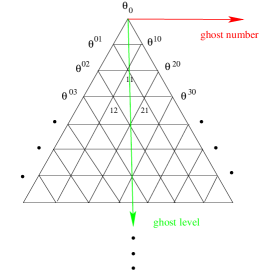
Figure 2: infinite pyramid of ghosts

Notice that $\pi$ and $\theta$ are shorthand notation for $\pi_{p,q}$ and $\theta^{p,q}$, where $p-q$ is the ghost number and $p+q$ is the ghost level. (Even level and odd level correspond to fermion and boson respectively.) The expression “$|_{>}$” means “ghosts only”.

Now we go to the Lagrangian form of the action for $x$. To obtain complete results for the amplitude rules, we need to keep terms in the Hamiltonian quadratic in the background fields. This has two unusual consequences: In the Lagrangian, (1) all these terms will become linear (as familiar from the bosonic case), and (2) such terms new to the supersymmetric case will appear only with $\dot{\theta}$.

Neglecting $ib\dot{c}$ and $F\cdot\hat{s}$ we see

$$-p\cdot\dot{x}+i\pi\dot{\theta}+{\textstyle{1\over 2}}(p+A)^{2}+W^{\alpha}[\pi_{0\alpha}+p^{a}(\gamma_{a}\theta_{0})_{\alpha}+A_{\alpha}]$$

$$\Rightarrow -{\textstyle{1\over 2}}\dot{x}^{2}+i\pi\dot{\theta}+A\cdot\dot{x}-iA_{\alpha}\dot{\theta}^{\alpha}+W^{\alpha}[\pi_{0\alpha}+(\dot{x}-A)\cdot(\gamma\theta_{0})_{\alpha}-{\textstyle{1\over 2}}(\gamma\theta)_{\alpha}\cdot W\gamma\theta]$$

By redefining $\pi_{0\alpha}\Rightarrow\pi_{0\alpha}+A\cdot(\gamma\theta_{0})_{\alpha}+{\textstyle{1\over 2}}(\gamma\theta_{0})_{\alpha}\cdot W\gamma\theta_{0}$ (deformed only with gauge fields) we get

$$-{\textstyle{1\over 2}}\dot{x}^{2}+i\pi\dot{\theta}-A_{\alpha}i\dot{\theta}_{0}^{\alpha}+A\cdot(\dot{x}+i\theta_{0}\gamma\dot{\theta_{0}})+W^{\alpha}[\pi_{0\alpha}+\dot{x}\cdot(\gamma\theta_{0})_{\alpha}+{\textstyle{i\over 2}}(\gamma\theta_{0})_{\alpha}\cdot\theta_{0}\gamma\dot{\theta}_{0}]$$

The background terms then give the vertex operator

$$V = A^{A}j_{A}$$ (A.1.2)

$$= A_{\alpha}\omega^{\alpha}+A^{a}p_{a}+W^{\alpha}d_{\alpha}+{\textstyle{1\over 2}}F^{ab}\hat{s}_{ba}$$

where

$$d_{\alpha} = \pi_{0\alpha}+\dot{x}\cdot(\gamma\theta_{0})_{\alpha}+{\textstyle{i\over 2}}(\gamma\theta_{0})_{\alpha}\cdot\theta_{0}\gamma\dot{\theta}_{0}$$

$$p_{a} = \dot{x}+i\theta_{0}\gamma\dot{\theta_{0}}$$

$$\omega^{\alpha} = -i\dot{\theta}_{0}^{\alpha}$$

$$\hat{s}_{ab} = \theta\gamma_{ab}\pi|_{>}$$ (A.1.3)

The fact that $\dot{\theta}$ vanishes by its free field equations is related to the fact that its contraction with $\pi$ gives a $\delta(z)$, canceling a (spacetime) propagator, and thus contracting two 3-point vertices into a 4-point vertex. Thus, they originate from terms in the Hamiltonian quadratic in background fields. The string vertex operator is the same, with the $z$ derivative replaced with the left- or right-handed worldsheet derivative.

In our previous paper [5] the background coupling had additional terms involving the expression $R^{a}$, quadratic in ghost $\theta$’s. These terms never contribute to amplitudes because there are no ghost $\pi$’s to cancel them. ($\hat{s}$ has a ghost $\pi$, but together with a ghost $\theta$.) This is also true for the superstring.

A.2 Superstring

Like the case of the superparticle, the gauge fixed action for the superstring comes from $\{\int b,Q_{sstring}\}$, adding first-order terms: without background,

$$S_{GF} = \int d^{2}z~{}\hat{P}^{m}\partial_{m}X-{\textstyle{1\over 2}}\eta_{mn}\hat{P}^{m}\hat{P}^{n}+i\sqrt{2}\sum_{\pm}\partial_{\pm}c^{\pm}b_{\pm\pm}+i\sqrt{2}\sum_{\pm}\partial_{\pm}\theta^{\pm}\pi^{\pm}$$

The $\sqrt{2}$ comes from $\partial_{\pm}=(1/\sqrt{2})(\partial_{0}\pm\partial_{1})$.

We can introduce the background as for the particle case:

$$V = A^{A}J_{A}$$ (A.2.1)

$$= A_{\alpha}\Omega^{\alpha}+A^{a}P_{a}+W^{\alpha}D_{\alpha}+{\textstyle{1\over 2}}F^{ab}\hat{S}_{ba}$$

where

$$D_{\alpha} = \pi_{0\alpha}+(\gamma^{a}\theta_{0})_{\alpha}\partial X_{a}+i{\textstyle{1\over 2}}(\gamma^{a}\theta_{0})_{\alpha}\theta_{0}\gamma_{a}\partial\theta_{0}$$

$$P_{a} = \partial X_{a}+i\theta_{0}\gamma_{a}\partial\theta_{0}$$

$$\Omega_{\alpha} = -i\partial\theta_{0\alpha}$$

$$\hat{S}_{ab} = \theta\gamma_{ab}\pi|_{>}$$ (A.2.2)

Appendix B Current algebra

The operator (affine Lie) algebra remains simple because the currents are no more than cubic in the fundamental variables:

$$J_{A}(z_{1})J_{B}(z_{2})=G_{AB}^{\prime}(z_{1}-z_{2}){f_{AB}}^{C}[z^{\prime}]J_{C}(z^{\prime})+G_{AB}^{\prime\prime}(z_{1}-z_{2})\mbox{\boldmath$\eta$}_{AB}+::J_{A}(z_{1})J_{B}(z_{2})::$$ (B.1)

where $J_{A}$ has zero-modes $j_{A}$, of which only $p_{a}$ and $d_{\alpha}$ act nontrivially on $A^{A}$, and $G_{AB}$ is the relevant Green function. For example, $G^{(n)}_{ab}=G^{(n)}_{x}$ and $G^{(n)}_{\alpha\beta}=G^{(n-1)}_{\theta}$. The various definitions are

$${f_{\alpha\beta}}^{a}[z]P_{a}(z) \equiv \gamma^{a}_{\alpha\beta}[P_{a}(z_{\alpha})+P_{a}(z_{\beta})]$$

$$f_{a\alpha\beta}[z]\Omega^{\beta}(z) \equiv 2\gamma_{a\alpha\beta}\Omega^{\beta}(z_{a})$$

$$f_{\alpha a\beta}[z]\Omega^{\beta}(z) \equiv -2\gamma_{a\alpha\beta}\Omega^{\beta}(z_{a})$$

$$\mbox{\boldmath$\eta$}_{\alpha}{}^{\beta} = -i\delta_{\alpha}^{\beta}$$

$$\mbox{\boldmath$\eta$}^{\beta}{}_{\alpha} = i\delta_{\alpha}^{\beta}$$

$$\mbox{\boldmath$\eta$}_{ab} = -\eta_{ab}$$

otherwise vanish

and

$$::J_{A}(z_{1})J_{B}(z_{2})::A^{C} \equiv :J_{A}(z_{1})J_{B}(z_{2}):A^{C}$$

$$J_{A}(z_{1})A^{B}(z_{2}) = G_{AB}^{\prime}(z_{1}-z_{2})(j_{A}A^{B})(z_{2})+\mathopen{:}J_{A}(z_{1})A^{B}(z_{2})\mathclose{:}$$

$$A^{A}(z_{1})A^{B}(z_{2}) = e^{-k_{1}\cdot k_{2}G_{x}(z_{1}-z_{2})}\mathopen{:}A^{A}(z_{1})A^{B}(z_{2})\mathclose{:}$$

$$::J_{A}(z_{1})J_{B}(z_{2})::J_{C}(z_{3}) \equiv (-1)^{BC}G_{AC}^{\prime}(z_{1}-z_{3}){f_{AC}}^{D}[z^{\prime}]J_{D}(z^{\prime})J_{C}(z_{3})$$ (B.2)

$$+G_{BC}^{\prime}(z_{2}-z_{3}){f_{BC}}^{D}[z^{\prime}]J_{A}(z_{1})J_{D}(z^{\prime})$$

$$+(-1)^{BC}G_{AC}^{\prime}(z_{1}-z_{3}){f_{AC}}^{D}[z^{\prime}]::J_{D}(z^{\prime})J_{C}(z_{3})::$$

$$+G_{BC}^{\prime}(z_{2}-z_{3}){f_{BC}}^{D}[z^{\prime}]::J_{A}(z_{1})J_{D}(z^{\prime})::$$

$$+::J_{A}(z_{1})J_{B}(z_{2})J_{C}(z_{3})::$$

It is then straightforward to get (2.2), which is all that is needed in amplitude calculations.

Appendix C Component expansions

The $\theta$ expansion of the superfields follows directly from the constraints on the (super)field strengths

$$~{}[\nabla_{a},\nabla_{b}]~{} = ~{}F_{ab}$$

$$\{\nabla_{0\alpha},\nabla_{0\beta}\}~{} = ~{}2\gamma_{a\alpha\beta}\nabla^{a}$$

$$~{}[\nabla_{0\alpha},\nabla_{a}]~{} = 2\gamma_{a\alpha\beta}W^{\beta}$$

and the Bianchi identities that follow from them.

Although in practice we perform component expansions by evaluating spinor derivatives at $\theta=0$, we can also directly expand superfields in $\theta$. In a Wess-Zumino gauge we have:

$$F_{ab}~{} = ~{}{\buildrel\mkern 2.5mu\circ\mkern-2.5mu\over{F}}{}_{ab}$$

$$W^{\alpha} = {\buildrel\mkern 2.5mu\circ\mkern-2.5mu\over{W}}{}^{\alpha}+~{}{\textstyle{1\over 2}}(\gamma^{ab}\theta_{0})^{\alpha}{\buildrel\mkern 2.5mu\circ\mkern-2.5mu\over{F}}{}_{ab}$$

$$A_{a} = {\buildrel\mkern 2.5mu\circ\mkern-2.5mu\over{A}}{}_{a}~{}+~{}2\theta_{0}\gamma_{a}{\buildrel\mkern 2.5mu\circ\mkern-2.5mu\over{W}}+~{}{\textstyle{1\over 2}}\theta_{0}\gamma_{a}\gamma^{bc}\theta_{0}~{}{\buildrel\mkern 2.5mu\circ\mkern-2.5mu\over{F}}{}_{bc}$$

$$A_{\alpha} = ~{}(\gamma^{a}\theta_{0})_{\alpha}{\buildrel\mkern 2.5mu\circ\mkern-2.5mu\over{A}}{}_{a}~{}+~{}{\textstyle{4\over 3}}(\gamma^{a}\theta_{0})_{\alpha}\theta_{0}\gamma_{a}{\buildrel\mkern 2.5mu\circ\mkern-2.5mu\over{W}}+~{}{\textstyle{1\over 4}}(\gamma^{a}\theta_{0})_{\alpha}\theta_{0}\gamma_{a}\gamma^{bc}\theta_{0}{\buildrel\mkern 2.5mu\circ\mkern-2.5mu\over{F}}{}_{bc}\qquad$$

where $\circ$ indicates $\theta_{0}$ independence, and we have expanded only to constant field strengths $W$ and $F$, which is sufficient for lower-point diagrams because of the deficiency of $\pi$’s. The vertex operator $V=V_{B}+V_{F}$ for the superparticle is then :

$$V_{B} = i{\buildrel\mkern 2.5mu\circ\mkern-2.5mu\over{A}}\cdot\dot{x}+{\textstyle{1\over 2}}{\buildrel\mkern 2.5mu\circ\mkern-2.5mu\over{F}}{}^{ab}\theta\gamma_{ba}\pi$$

$$V_{F} = {\buildrel\mkern 2.5mu\circ\mkern-2.5mu\over{W}}{}^{\alpha}[\pi_{0\alpha}-i\dot{x}\cdot(\gamma\theta_{0})_{\alpha}-{\textstyle{i\over 6}}(\gamma_{a}\theta_{0})_{\alpha}\theta_{0}\gamma^{a}\dot{\theta}_{0}]$$ (C.1)

Here $\theta\gamma_{ab}\pi$ includes the physical $\pi_{0},\theta_{0}$. (In terms of superfields and currents we hide this physical $\pi_{0},\theta_{0}$ in $W^{\alpha}$ and $D_{\alpha}$. Then $\hat{S}$ has only ghost number non-zero $\pi,\theta$.) Notice that the spinor vertex is the supersymmetry generator $q_{\alpha}$, which will happen again in the superstring case. Inserting plane waves for the fields,

$$V_{B} = A_{a}(i\dot{x}^{a}+\theta\gamma^{ab}\pi k_{b})e^{ik\cdot x}$$ (C.2)

$$V_{F} = w^{\alpha}[\pi_{0\alpha}-i\dot{x}\cdot(\gamma\theta_{0})_{\alpha}-{\textstyle{i\over 6}}(\gamma_{a}\theta_{0})_{\alpha}\theta_{0}\gamma^{a}\dot{\theta}_{0}]e^{ik\cdot x}$$ (C.3)

The superstring vertices are essentially the same.

Appendix D Loop review

D.1 Superparticle

Since our theory is 1st-quantized, we should calculate amplitudes in terms of worldline Green functions with periodic boundary conditions [21]. So our partition function with imaginary time is

$$\mathcal{N}\int_{0}^{\infty}\frac{dT}{T}\int\mathcal{D}X~{}\mathcal{D}c~{}\mathcal{D}b~{}\mathcal{D}\theta~{}\mathcal{D}\pi~{}Tr~{}e^{-\int^{T}_{0}dz\ L_{\theta}}$$ (D.1.1)

where

$$\mathcal{N}=\int\mathcal{D}P\ e^{-\int^{T}_{0}dzP^{2}/2}$$ (D.1.2)

and $\int dT/T$ comes from the Schwinger proper-time integral representation of the 1-loop vacuum energy $-Tr[\ln(-\Box)]$.

Since this is a 1-loop amplitude, we should impose periodic boundary conditions, on both $X$ and $\theta$ (to preserve supersymmetry):

$$X(T)=X(0),\quad\quad\theta(T)=\theta(0)$$ (D.1.3)

This boundary condition also results in a supertrace naturally in the loop amplitude.

In this setting the color-ordered, N-point, 1-loop amplitude of the superparticle can be written as:

$$A_{N}=G_{N}\int_{0}^{\infty}dT\ (2\pi T)^{-D/2}\int_{0\leq z_{r}\leq z_{r+1}\leq z_{N}=T\leq\infty}d^{N-1}z_{i}\ K_{N}\ e^{-\sum_{1\leq r<s\leq N}k_{r}\cdot k_{s}G_{rs}}$$ (D.1.4)

The factor $(2\pi T)^{-D/2}$ comes from $\mathcal{N}\int\mathcal{D}Xe^{-\int\dot{X}^{2}/2}$. The $z_{i}$ integration factors come from the Nth order expansion of the vertex operator. The worldline Green function $G(z_{s}-z_{r})$ is given in (4.2). Examples of the kinematic factor $K_{N}$ are given in section 5. The factor $G_{N}$ is the trace of group generators in a given ordering.

D.2 Superstrings

The procedure is almost identical to the particle case. One difference is that our Green functions are now doubly periodic:

$$G^{x}(z)=G^{x}(z+2\pi i)=G^{x}(z+T)$$

$$G^{\theta}(z)=G^{\theta}(z+2\pi i)=G^{\theta}(z+T)$$ (D.2.1)

Again this periodic boundary condition in both directions is required by supersymmetry. Also, there is a topological distinction among graphs, namely planar, nonplanar, and unorientable graphs. We will concentrate on the planar one here; the others follow from similar considerations.

We can write the color-ordered, N-point, 1-loop, superstring amplitude in a form identical to that of the particle case (D.1.4), but with the string Green function given in Appendix E. After the usual change of variables

$$\rho_{i}=e^{-z_{i}},\quad\quad w=\rho_{N}=e^{-T}$$ (D.2.2)

we have

$$G_{N}\int_{0}^{1}\frac{dw}{w}\left(\frac{-2\pi}{\ln w}\right)^{D/2}\int_{0\leq w\leq\rho_{r+1}\leq\rho_{r}\leq 1}\prod_{r=1}^{N-1}\frac{d\rho_{r}}{\rho_{r}}\ K_{N}\ e^{-\sum_{1\leq r<s\leq N}k_{r}\cdot k_{s}G_{rs}}$$ (D.2.3)

In the bosonic case there is a factor of $[f(w)]^{-D+2}$ coming from the partition function (and a $w$ from the tachyon mass) for $D$ $X$’s and the 2 reparametrization ghosts $b$ and $c$. In the supersymmetric case this is canceled (as in all superstring formulations) by an $[f(w)]^{(2^{D/2})(1-2+3-4+\cdots)}=[f(w)]^{2^{(D-4)/2}}$ which comes from the infinite pyramid of spinors, in $D=10$. However, the regularization introduces corrections to the spinor partition function:

$$\prod_{n}(1-w^{n})^{4}(1-w^{n})^{4}\Rightarrow\prod_{n}(1-w^{n+i\epsilon})^{4}(1-w^{n-i\epsilon})^{4}$$ (D.2.4)

The $\epsilon$ expansion of this partition function gives corrections to amplitudes. For example, in the 6-point, 1-loop amplitude we expect a term $\sim(1/\epsilon)^{6}(\epsilon^{2}\theta_{1}^{\prime\prime\prime}/\theta^{\prime}_{1})$, where the $(1/\epsilon)^{6}$ comes from 6 $G^{\theta}$’s and the $\epsilon^{2}\theta_{1}^{\prime\prime\prime}/\theta^{\prime}_{1}$ comes from expansion of the spinor partition function.

Appendix E Periodic Green functions

E.1 Second order

The general Fourier decomposition of a function in 2 dimensions with doubly periodic boundary conditions $((x,y)\simeq(x+2\pi,y)\simeq(x,y+2\pi\tau))$ for real $\tau=T/2\pi$ is

$$G(x-x^{\prime},y-y^{\prime})=\sum_{n,m}G_{n,m}~{}e^{in(x-x^{\prime})+im(y-y^{\prime})/\tau}$$ (E.1.1)

Then the $G_{n,m}$ for the Green function of the differential operator $-\partial^{2}_{x}-\partial^{2}_{y}+\epsilon^{2}$ is easily found to be

$$G_{n,m}=\frac{1}{2\pi\tau}\frac{1}{n^{2}+\frac{m^{2}}{\tau^{2}}+\epsilon^{2}}$$ (E.1.2)

For simplicity we can set $x^{\prime}=y^{\prime}=0$ by translational invariance. Using Schwinger proper-time parametrization we get

$$G(x,y)=\frac{1}{2\pi\tau}\sum_{n,m}\int_{0}^{\infty}ds~{}e^{-s(n^{2}+m^{2}/\tau^{2}+\epsilon^{2})+inx+imy/\tau}$$ (E.1.3)

Next using Jacobi’s transform

$$\sum_{m}~{}e^{-sm^{2}/\tau^{2}+imy/\tau}=\tau\sqrt{\frac{\pi}{s}}\sum_{m}~{}e^{-(2\pi m-y/\tau)^{2}\tau^{2}/4s}$$

we get

$$G(x,y)=\frac{1}{2\pi}\sum_{n,m}\int_{0}^{\infty}ds~{}\sqrt{\frac{\pi}{s}}~{}e^{-(2\pi m-y/\tau)^{2}\tau^{2}/4s-s(n^{2}+\epsilon^{2})+inx}$$ (E.1.4)

Then using

$$\int^{\infty}_{0}ds~{}s^{\alpha-1}~{}e^{-ps-q/s}=2\left(\frac{q}{p}\right)^{\alpha/2}K_{\alpha}(2\sqrt{pq})$$

we get

$$G(x,y)=\frac{1}{\sqrt{2\pi}}\sum_{n,m}\left(\frac{(2\pi m\tau-y)^{2}}{n^{2}+\epsilon^{2}}\right)^{1/4}e^{inx}K_{1/2}\left(\sqrt{(2\pi m\tau-y)^{2}(n^{2}+\epsilon^{2})}\right)$$ (E.1.5)

Also using $K_{1/2}(z)=\sqrt{\pi/2z}e^{-z}$ we get

$$G(x,y) = \frac{1}{2}\sum_{n,m}\frac{1}{\sqrt{n^{2}+\epsilon^{2}}}e^{-|2\pi m\tau-y|\sqrt{n^{2}+\epsilon^{2}}+inx}$$ (E.1.6)

$$= \frac{1}{2\epsilon}e^{-\epsilon|y|}+\frac{1}{2\epsilon}\sum_{m\neq 0}e^{-\epsilon|2\pi m\tau-y|}+\frac{1}{2}\sum_{n\neq 0}\frac{1}{\sqrt{n^{2}+\epsilon^{2}}}e^{-|y|\sqrt{n^{2}+\epsilon^{2}}+inx}$$

$$\frac{1}{2}\sum_{n,m\neq 0}\frac{1}{\sqrt{n^{2}+\epsilon^{2}}}e^{-|2\pi m\tau-y|\sqrt{n^{2}+\epsilon^{2}}+inx}$$

Now let’s transform each sum into a sum over positive integers only:

$$\frac{1}{2\epsilon}\sum_{m\neq 0}e^{-\epsilon|2\pi m\tau-y|} = \frac{1}{\epsilon}\cosh(\epsilon y)\sum^{\infty}_{m=1}e^{-2\pi m\tau\epsilon}$$ (E.1.7)

$$= \frac{1}{2\epsilon}e^{-\pi\tau\epsilon}\frac{\cosh(\epsilon y)}{\sinh(\pi\tau\epsilon)}$$

$$\frac{1}{2}\sum_{n\neq 0}{\textstyle{1\over\sqrt{n^{2}+\epsilon^{2}}}}e^{-|y|\sqrt{n^{2}+\epsilon^{2}}~{}+~{}inx}=\frac{1}{2}\sum_{n=1}^{\infty}{\textstyle{1\over\sqrt{n^{2}+\epsilon^{2}}}}(\lambda_{n}^{n}+c.c.)$$ (E.1.8)

$$\frac{1}{2}\sum_{n,m\neq 0}{\textstyle{1\over\sqrt{n^{2}+\epsilon^{2}}}}e^{-|2\pi m\tau-y|\sqrt{n^{2}+\epsilon^{2}}~{}+~{}inx}=\frac{1}{2}\sum_{n,m=1}^{\infty}{\textstyle{1\over\sqrt{n^{2}+\epsilon^{2}}}}w^{mn}_{n}(\rho_{n}^{n}+\rho_{n}^{-n}+c.c.)$$ (E.1.9)

where

$$\ln\lambda_{n} = i\left(x+i|y|\sqrt{1+\frac{\epsilon^{2}}{n^{2}}}\right)$$

$$\ln\rho_{n} = i\left(x+iy\sqrt{1+\frac{\epsilon^{2}}{n^{2}}}\right)$$

$$w_{n} = e^{-2\pi\tau\sqrt{1+\epsilon^{2}/n^{2}}}$$

We can subtract out $G$ for the particle from $G(x,y)$, which includes the part divergent as $\epsilon\rightarrow 0$:

$$\frac{1}{2\epsilon}\frac{\cosh[\epsilon(|y|-\pi\tau)]}{\sinh(\pi\tau\epsilon)}$$ (E.1.11)

The remainder is

$$\frac{1}{2}\sum_{n=1}^{\infty}{\textstyle{1\over\sqrt{n^{2}+\epsilon^{2}}}}(\lambda_{n}^{n}+c.c.)+\frac{1}{2}\sum_{n,m=1}^{\infty}{\textstyle{1\over\sqrt{n^{2}+\epsilon^{2}}}}w^{mn}_{n}(\rho_{n}^{n}+\rho_{n}^{-n}+c.c)$$ (E.1.12)

In the $\epsilon\rightarrow 0$ limit ($w_{n}\rightarrow w=e^{-T},\lambda_{n}\rightarrow\lambda,\rho_{n}\rightarrow\rho=e^{-z},z=y-ix$), using

$$\sum_{n=1}^{\infty}\frac{x^{n}}{n}=-\ln(1-x)\\$$

we get for the remainder

$$-\ln|1-\lambda|-\sum_{m=1}^{\infty}\ln|(1-w^{m}\rho)(1-w^{m}\rho^{-1})|$$

$$\quad\quad=-\frac{[Re(z)]^{2}}{2T}-\frac{1}{2}\ln|\lambda|-\ln|f(w)^{2}|+G^{x}_{un}$$

where (assuming $|y|=y$ for simplicity)

$$G^{x}_{un}(z,T) = -\ln\left|\frac{2\pi\theta_{1}(\frac{iz}{2\pi}|{\textstyle{iT\over 2\pi}})}{\theta^{\prime}_{1}(0|{\textstyle{iT\over 2\pi}})}\right|+\frac{[Re(z)]^{2}}{2T}$$

$$\theta_{1}({\textstyle{iz\over 2\pi}}|{\textstyle{iT\over 2\pi}}) = -iw^{1/8}(\rho^{1/2}-\rho^{-1/2})\prod_{m=1}^{\infty}(1-w^{m}\rho)(1-w^{m}\rho^{-1})(1-w^{m})$$

$$\theta^{\prime}_{1}(0|{\textstyle{iT\over 2\pi}}) = 2\pi w^{1/8}f^{3}(w),\qquad f(w)=\prod_{m=1}^{\infty}(1-w^{m})$$

and $G^{x}_{un}$ is the unregularized Green function with the usual $T$-dependent “constant” added to normalize its short distance behavior to be the same as that of the tree case (see, e.g., [22]).

Combining the two parts we get

$$G(\rho) = \frac{1}{T\epsilon^{2}}+\frac{y^{2}}{2T}-\frac{y}{2}+\frac{T}{12}+\mathcal{O}(\epsilon)$$ (E.1.13)

$$+\frac{1}{2}Re\left(\frac{\ln^{2}\rho}{\ln w}\right)-\frac{1}{2}\ln|\rho|-\ln|[f(w)]^{2}|+G^{x}_{un}+\mathcal{O}(\epsilon)$$

$$= \frac{1}{T\epsilon^{2}}-{1\over 12}\ln|w[f(w)]^{24}|+G^{x}_{un}+\mathcal{O}(\epsilon)$$

The first term is the zero-mode behavior, and the second term is a constant that won’t contribute to massless amplitudes (because of derivatives and $k^{2}=0$; the non-$f$ piece is the same as for the particle).

E.2 First order

The worldsheet Green function for $\theta$ can be obtained by differentiating that for $X$. However, to be careful about zero-modes some modification is needed. For the 1st-order differential operator $-i(\partial_{y}-i\partial_{x}+\epsilon)$ we find the mode sum of the Green function

$$G^{\theta} = {i\over T}\sum_{m,n}\frac{-im/\tau+n+\epsilon}{m^{2}/\tau^{2}+(n+\epsilon)^{2}}e^{inx+imy/\tau}$$

$$= i(-\partial_{y}-i\partial_{x}+\epsilon)\frac{1}{2\pi\tau}\sum_{m,n}\frac{1}{m^{2}/\tau^{2}+(n+\epsilon)^{2}}e^{inx+imy/\tau}$$

where the $\epsilon$ in the numerator is nontrivial because the second-order Green function has a $1/\epsilon$ pole. The above sum is almost identical to the second-order case except for the change $n^{2}+\epsilon^{2}\Rightarrow(n+\epsilon)^{2}$. Therefore we can write the first-order Green function as

$$G^{\theta} = i(-\partial_{y}-i\partial_{x}+\epsilon)\left[\frac{1}{2\epsilon}\frac{\cosh[\epsilon(|y|-\pi\tau)]}{\sinh(\pi\tau\epsilon)}+\frac{1}{2}\sum_{n=1}^{\infty}\frac{1}{n+\epsilon}(\lambda_{n}^{n}+c.c.)\right.$$ (E.2.1)

$$\left.\hskip 28.45274pt+\frac{1}{2}\sum_{n,m=1}^{\infty}\frac{1}{n+\epsilon}w^{mn}_{n}(\rho_{n}^{n}+\rho_{n}^{-n}+c.c.)\right]$$

where

$$\ln\lambda_{n} = i\left[x+i|y|\left(1+\frac{\epsilon}{n}\right)\right]$$

$$\ln\rho_{n} = i\left[x+iy\left(1+\frac{\epsilon}{n}\right)\right]$$

$$w_{n} = e^{-2\pi\tau(1+\epsilon/n)}$$

Hence it has a less divergent leading term followed by the expected differentiated second-order Green function:

$$G^{\theta} = {i\over T\epsilon}+\sum_{n=0}^{\infty}G^{\theta}_{n}\epsilon^{n}$$ (E.2.2)

$$= {i\over T\epsilon}+i(\partial_{y}+i\partial_{x})G^{x}_{0}+\mathcal{O}(\epsilon)$$

Appendix F Super amplitudes

F.1 Super tree

In this section we give some details of the calculation of 3-point tree and 4-point 1-loop super amplitudes.

We will concentrate on terms which give fermion contributions. In (3.3) only $C,D,$ and $E$ give the $AWW$ amplitude. Let’s consider $A(1)W(2)W(3)$, for example. Using (2.2),(B) we get for the tree (no fermion zero-mode regularization)

$$\langle P_{a}(1)P_{b}(2)\rangle = -\eta_{ab}{\textstyle{1\over(z_{1}-z_{2})^{2}}}$$

$$\langle D_{\alpha}(1)\Omega^{\beta}(2)\rangle = \delta_{\alpha}^{\beta}{\textstyle{1\over(z_{1}-z_{2})^{2}}}$$

$$\langle P_{a}(1)D_{\alpha}(2)D_{\beta}(3)\rangle = -i\gamma_{a\alpha\beta}[{\textstyle{2\over z_{1}-z_{2}}}{\textstyle{1\over(z_{1}-z_{3})^{2}}}-{\textstyle{2\over z_{1}-z_{3}}}{\textstyle{1\over(z_{2}-z_{1})^{2}}}$$ (F.1.1)

$$-{\textstyle{1\over z_{2}-z_{3}}}({\textstyle{1\over(z_{1}-z_{2})^{2}}}+{\textstyle{1\over(z_{1}-z_{3})^{2}}})]$$

Then we see in the Wess-Zumino gauge ($A_{\alpha}=\gamma^{a}_{\alpha\beta}\theta^{\beta}A^{a}+\mathcal{O}(\theta^{2})+\cdots$, etc.)

$$C:(PPD) : -\langle P_{a}(1)P_{b}(2)\rangle A^{a}(1)(D_{\alpha}(3)A^{b}(2))W^{\alpha}(3)$$

$$= -i{\textstyle{1\over(z_{1}-z_{2})^{2}}}{\textstyle{1\over z_{3}-z_{2}}}A^{a}(1)(d_{\alpha}A_{a}(2))W^{\alpha}(3)$$

$$= -i{\textstyle{1\over(z_{1}-z_{2})^{2}}}{\textstyle{2\over z_{3}-z_{2}}}A^{a}(1)W(2)\gamma_{a}W(3)$$

$$(PDP) : -\langle P_{a}(1)P_{b}(3)\rangle A^{a}(1)(D_{\alpha}(2)A^{b}(3))W^{\alpha}(2)$$

$$= -i{\textstyle{1\over(z_{1}-z_{3})^{2}}}{\textstyle{2\over z_{2}-z_{3}}}A^{a}(1)W(3)\gamma_{a}W(2)$$

$$D:(PDD) : -\langle P_{a}(1)D_{\alpha}(2)D_{\beta}(3)\rangle A^{a}(1)W^{\alpha}(2)W^{\beta}(3)$$

$$= i[{\textstyle{2\over z_{1}-z_{2}}}{\textstyle{1\over(z_{1}-z_{3})^{2}}}-{\textstyle{2\over z_{1}-z_{3}}}{\textstyle{1\over(z_{2}-z_{1})^{2}}}$$

$$-{\textstyle{1\over z_{2}-z_{3}}}({\textstyle{1\over(z_{1}-z_{2})^{2}}}+{\textstyle{1\over(z_{1}-z_{3})^{2}}})]A(1)\cdot W(2)\gamma W(3)$$

$$E:(\Omega DD) : \langle\Omega^{\alpha}(1)D_{\beta}(2)\rangle(D_{\gamma}(3)A_{\alpha}(1))W^{\beta}(2)W^{\gamma}(3)$$ (F.1.2)

$$-\langle\Omega^{\alpha}(1)D_{\gamma}(3)\rangle(D_{\beta}(2)A_{\alpha}(1))W^{\beta}(2)W^{\gamma}(3)$$

$$= i\left[-{\textstyle{1\over(z_{1}-z_{2})^{2}}}{\textstyle{1\over z_{3}-z_{1}}}+{\textstyle{1\over(z_{1}-z_{3})^{2}}}{\textstyle{1\over z_{2}-z_{1}}}\right]A(1)\cdot W(2)\gamma W(3)$$

This reduces to (3.3).

F.2 1 loop : 2 fermions + 2 vectors

We will concentrate on the case where the fermions are at both ends. The other case can be easily obtained by permutation. There are two kinds of contributions: $W(dW)(dddW)W$ (with $WF(ddF)W$) and $W(dW)(dW)(ddW)$ (and corresponding $W(dW)F(dF)$). The $W^{2}F^{2}$ contribution gives a GP sum with the corresponding $W^{2}(dW)^{2}$ as usual. The explicit formula is

$$A: - W^{\alpha}(1)\left(d_{\gamma}W^{\beta}(2)\right)\left({\textstyle{1\over 3!}}d_{[\delta}d_{\alpha}d_{\beta]}W^{\gamma}(3)\right)W^{\delta}(4)$$

$$+ {\textstyle{3\over 16}}tr(\gamma_{ab}\gamma_{cd})W^{\alpha}(1)F^{ab}(2)\left({\textstyle{1\over 2!}}d_{[\delta}d_{\alpha]}F^{cd}(3)\right)W^{\delta}(4)$$

$$B: - W^{\alpha}(1)\left({\textstyle{1\over 3!}}d_{[\delta}d_{\alpha}d_{\gamma]}W^{\beta}(2)\right)\left(d_{\beta}W^{\gamma}(3)\right)W^{\delta}(4)$$

$$+ {\textstyle{3\over 16}}tr(\gamma_{ab}\gamma_{cd})W^{\alpha}(1)\left({\textstyle{1\over 2!}}d_{[\delta}d_{\alpha]}F^{ab}(2)\right)F^{cd}(3)W^{\delta}(4)$$

$$C: - W^{\alpha}(1)\left(d_{\alpha}W^{\beta}(2)\right)\left(d_{\delta}W^{\gamma}(3)\right)\left({\textstyle{1\over 2!}}d_{[\beta}d_{\gamma]}W^{\delta}(4)\right)$$

$$+ {\textstyle{3\over 16}}tr(\gamma_{ab}\gamma_{cd})W^{\alpha}\left(d_{\alpha}W^{\beta}(2)\right)F^{ab}(3)\left(d_{\beta}F^{cd}(4)\right)$$

$$D: - W^{\alpha}(1)\left(d_{\delta}W^{\beta}(2)\right)\left(d_{\alpha}W^{\gamma}(3)\right)\left({\textstyle{1\over 2!}}d_{[\gamma}d_{\beta]}W^{\delta}(4)\right)$$

$$+ {\textstyle{3\over 16}}tr(\gamma_{ab}\gamma_{cd})W^{\alpha}(1)F^{ab}(2)\left(d_{\alpha}W^{\gamma}(3)\right)\left(d_{\gamma}F^{cd}(4)\right)$$

$$E: \left(d_{\beta}d_{\gamma}W^{\alpha}(1)\right)\left(d_{\delta}W^{\beta}(2)\right)\left(d_{\alpha}W^{\gamma}(3)\right)W^{\delta}(4)$$

$$- {\textstyle{3\over 16}}tr(\gamma_{ab}\gamma_{cd})\left(d_{\beta}F^{ab}(1)\right)\left(d_{\delta}W^{\beta}(2)\right)F^{cd}(3)W^{\delta}(4)$$

$$F: \left(d_{\gamma}d_{\beta}W^{\alpha}(1)\right)\left(d_{\alpha}W^{\beta}(2)\right)\left(d_{\delta}W^{\gamma}(3)\right)W^{\delta}(4)$$ (F.2.1)

$$- {\textstyle{3\over 16}}tr(\gamma_{ab}\gamma_{cd})\left(d_{\gamma}F^{ab}(1)\right)F^{cd}(2)\left(d_{\delta}W^{\gamma}(3)\right)W^{\delta}(4)$$

$A$ and $B$ vanish due to a GP sum. $C+D$ and $E+F$ give identical contributions, using integration by parts (momentum conservation) and the (free) $W$ field equation $\mathchoice{\partial\kern-5.30904pt{\hbox to5.30904pt{\hfil$\displaystyle{/}$\hfil}}}{\partial\kern-5.30904pt{\hbox to5.30904pt{\hfil$\textstyle{/}$\hfil}}}{\partial\kern-3.71632pt{\hbox to3.71632pt{\hfil$\scriptstyle{/}$\hfil}}}{\partial\kern-2.65451pt{\hbox to2.65451pt{\hfil$\scriptscriptstyle{/}$\hfil}}}W=0$. The results are given in (5.3).

These results appear in the literature in forms where neither gauge invariance nor permutation symmetry (relating FFBB and FBFB) is manifest, which we now provide for comparison. When written in terms of each momentum and gauge field, the results are (before applying integration by parts)

$$C: -{\textstyle{1\over 2}}k_{1}\cdot k_{2}W(1)\mathchoice{A\kern-7.50002pt{\hbox to7.50002pt{\hfil$\displaystyle{/}$\hfil}}}{A\kern-7.50002pt{\hbox to7.50002pt{\hfil$\textstyle{/}$\hfil}}}{A\kern-5.25pt{\hbox to5.25pt{\hfil$\scriptstyle{/}$\hfil}}}{A\kern-3.75pt{\hbox to3.75pt{\hfil$\scriptscriptstyle{/}$\hfil}}}_{2}\mathchoice{k\kern-5.52084pt{\hbox to5.52084pt{\hfil$\displaystyle{/}$\hfil}}}{k\kern-5.52084pt{\hbox to5.52084pt{\hfil$\textstyle{/}$\hfil}}}{k\kern-3.86458pt{\hbox to3.86458pt{\hfil$\scriptstyle{/}$\hfil}}}{k\kern-2.7604pt{\hbox to2.7604pt{\hfil$\scriptscriptstyle{/}$\hfil}}}_{2}\mathchoice{A\kern-7.50002pt{\hbox to7.50002pt{\hfil$\displaystyle{/}$\hfil}}}{A\kern-7.50002pt{\hbox to7.50002pt{\hfil$\textstyle{/}$\hfil}}}{A\kern-5.25pt{\hbox to5.25pt{\hfil$\scriptstyle{/}$\hfil}}}{A\kern-3.75pt{\hbox to3.75pt{\hfil$\scriptscriptstyle{/}$\hfil}}}_{3}W(4)+{\textstyle{1\over 2}}A_{3}\cdot k_{4}W(1)\mathchoice{A\kern-7.50002pt{\hbox to7.50002pt{\hfil$\displaystyle{/}$\hfil}}}{A\kern-7.50002pt{\hbox to7.50002pt{\hfil$\textstyle{/}$\hfil}}}{A\kern-5.25pt{\hbox to5.25pt{\hfil$\scriptstyle{/}$\hfil}}}{A\kern-3.75pt{\hbox to3.75pt{\hfil$\scriptscriptstyle{/}$\hfil}}}_{2}\mathchoice{k\kern-5.52084pt{\hbox to5.52084pt{\hfil$\displaystyle{/}$\hfil}}}{k\kern-5.52084pt{\hbox to5.52084pt{\hfil$\textstyle{/}$\hfil}}}{k\kern-3.86458pt{\hbox to3.86458pt{\hfil$\scriptstyle{/}$\hfil}}}{k\kern-2.7604pt{\hbox to2.7604pt{\hfil$\scriptscriptstyle{/}$\hfil}}}_{2}\mathchoice{k\kern-5.52084pt{\hbox to5.52084pt{\hfil$\displaystyle{/}$\hfil}}}{k\kern-5.52084pt{\hbox to5.52084pt{\hfil$\textstyle{/}$\hfil}}}{k\kern-3.86458pt{\hbox to3.86458pt{\hfil$\scriptstyle{/}$\hfil}}}{k\kern-2.7604pt{\hbox to2.7604pt{\hfil$\scriptscriptstyle{/}$\hfil}}}_{3}W(4)$$

$$D: -{\textstyle{1\over 2}}k_{1}\cdot k_{3}W(1)\mathchoice{A\kern-7.50002pt{\hbox to7.50002pt{\hfil$\displaystyle{/}$\hfil}}}{A\kern-7.50002pt{\hbox to7.50002pt{\hfil$\textstyle{/}$\hfil}}}{A\kern-5.25pt{\hbox to5.25pt{\hfil$\scriptstyle{/}$\hfil}}}{A\kern-3.75pt{\hbox to3.75pt{\hfil$\scriptscriptstyle{/}$\hfil}}}_{3}\mathchoice{k\kern-5.52084pt{\hbox to5.52084pt{\hfil$\displaystyle{/}$\hfil}}}{k\kern-5.52084pt{\hbox to5.52084pt{\hfil$\textstyle{/}$\hfil}}}{k\kern-3.86458pt{\hbox to3.86458pt{\hfil$\scriptstyle{/}$\hfil}}}{k\kern-2.7604pt{\hbox to2.7604pt{\hfil$\scriptscriptstyle{/}$\hfil}}}_{3}\mathchoice{A\kern-7.50002pt{\hbox to7.50002pt{\hfil$\displaystyle{/}$\hfil}}}{A\kern-7.50002pt{\hbox to7.50002pt{\hfil$\textstyle{/}$\hfil}}}{A\kern-5.25pt{\hbox to5.25pt{\hfil$\scriptstyle{/}$\hfil}}}{A\kern-3.75pt{\hbox to3.75pt{\hfil$\scriptscriptstyle{/}$\hfil}}}_{2}W(4)+{\textstyle{1\over 2}}A_{2}\cdot k_{4}W(1)\mathchoice{A\kern-7.50002pt{\hbox to7.50002pt{\hfil$\displaystyle{/}$\hfil}}}{A\kern-7.50002pt{\hbox to7.50002pt{\hfil$\textstyle{/}$\hfil}}}{A\kern-5.25pt{\hbox to5.25pt{\hfil$\scriptstyle{/}$\hfil}}}{A\kern-3.75pt{\hbox to3.75pt{\hfil$\scriptscriptstyle{/}$\hfil}}}_{3}\mathchoice{k\kern-5.52084pt{\hbox to5.52084pt{\hfil$\displaystyle{/}$\hfil}}}{k\kern-5.52084pt{\hbox to5.52084pt{\hfil$\textstyle{/}$\hfil}}}{k\kern-3.86458pt{\hbox to3.86458pt{\hfil$\scriptstyle{/}$\hfil}}}{k\kern-2.7604pt{\hbox to2.7604pt{\hfil$\scriptscriptstyle{/}$\hfil}}}_{3}\mathchoice{k\kern-5.52084pt{\hbox to5.52084pt{\hfil$\displaystyle{/}$\hfil}}}{k\kern-5.52084pt{\hbox to5.52084pt{\hfil$\textstyle{/}$\hfil}}}{k\kern-3.86458pt{\hbox to3.86458pt{\hfil$\scriptstyle{/}$\hfil}}}{k\kern-2.7604pt{\hbox to2.7604pt{\hfil$\scriptscriptstyle{/}$\hfil}}}_{2}W(4)$$

$$E: -{\textstyle{1\over 2}}k_{1}\cdot k_{3}W(4)\mathchoice{A\kern-7.50002pt{\hbox to7.50002pt{\hfil$\displaystyle{/}$\hfil}}}{A\kern-7.50002pt{\hbox to7.50002pt{\hfil$\textstyle{/}$\hfil}}}{A\kern-5.25pt{\hbox to5.25pt{\hfil$\scriptstyle{/}$\hfil}}}{A\kern-3.75pt{\hbox to3.75pt{\hfil$\scriptscriptstyle{/}$\hfil}}}_{2}\mathchoice{k\kern-5.52084pt{\hbox to5.52084pt{\hfil$\displaystyle{/}$\hfil}}}{k\kern-5.52084pt{\hbox to5.52084pt{\hfil$\textstyle{/}$\hfil}}}{k\kern-3.86458pt{\hbox to3.86458pt{\hfil$\scriptstyle{/}$\hfil}}}{k\kern-2.7604pt{\hbox to2.7604pt{\hfil$\scriptscriptstyle{/}$\hfil}}}_{2}\mathchoice{A\kern-7.50002pt{\hbox to7.50002pt{\hfil$\displaystyle{/}$\hfil}}}{A\kern-7.50002pt{\hbox to7.50002pt{\hfil$\textstyle{/}$\hfil}}}{A\kern-5.25pt{\hbox to5.25pt{\hfil$\scriptstyle{/}$\hfil}}}{A\kern-3.75pt{\hbox to3.75pt{\hfil$\scriptscriptstyle{/}$\hfil}}}_{3}W(1)+{\textstyle{1\over 2}}A_{3}\cdot k_{1}W(4)\mathchoice{A\kern-7.50002pt{\hbox to7.50002pt{\hfil$\displaystyle{/}$\hfil}}}{A\kern-7.50002pt{\hbox to7.50002pt{\hfil$\textstyle{/}$\hfil}}}{A\kern-5.25pt{\hbox to5.25pt{\hfil$\scriptstyle{/}$\hfil}}}{A\kern-3.75pt{\hbox to3.75pt{\hfil$\scriptscriptstyle{/}$\hfil}}}_{2}\mathchoice{k\kern-5.52084pt{\hbox to5.52084pt{\hfil$\displaystyle{/}$\hfil}}}{k\kern-5.52084pt{\hbox to5.52084pt{\hfil$\textstyle{/}$\hfil}}}{k\kern-3.86458pt{\hbox to3.86458pt{\hfil$\scriptstyle{/}$\hfil}}}{k\kern-2.7604pt{\hbox to2.7604pt{\hfil$\scriptscriptstyle{/}$\hfil}}}_{2}\mathchoice{k\kern-5.52084pt{\hbox to5.52084pt{\hfil$\displaystyle{/}$\hfil}}}{k\kern-5.52084pt{\hbox to5.52084pt{\hfil$\textstyle{/}$\hfil}}}{k\kern-3.86458pt{\hbox to3.86458pt{\hfil$\scriptstyle{/}$\hfil}}}{k\kern-2.7604pt{\hbox to2.7604pt{\hfil$\scriptscriptstyle{/}$\hfil}}}_{3}W(1)$$

$$F: -{\textstyle{1\over 2}}k_{1}\cdot k_{2}W(4)\mathchoice{A\kern-7.50002pt{\hbox to7.50002pt{\hfil$\displaystyle{/}$\hfil}}}{A\kern-7.50002pt{\hbox to7.50002pt{\hfil$\textstyle{/}$\hfil}}}{A\kern-5.25pt{\hbox to5.25pt{\hfil$\scriptstyle{/}$\hfil}}}{A\kern-3.75pt{\hbox to3.75pt{\hfil$\scriptscriptstyle{/}$\hfil}}}_{3}\mathchoice{k\kern-5.52084pt{\hbox to5.52084pt{\hfil$\displaystyle{/}$\hfil}}}{k\kern-5.52084pt{\hbox to5.52084pt{\hfil$\textstyle{/}$\hfil}}}{k\kern-3.86458pt{\hbox to3.86458pt{\hfil$\scriptstyle{/}$\hfil}}}{k\kern-2.7604pt{\hbox to2.7604pt{\hfil$\scriptscriptstyle{/}$\hfil}}}_{3}\mathchoice{A\kern-7.50002pt{\hbox to7.50002pt{\hfil$\displaystyle{/}$\hfil}}}{A\kern-7.50002pt{\hbox to7.50002pt{\hfil$\textstyle{/}$\hfil}}}{A\kern-5.25pt{\hbox to5.25pt{\hfil$\scriptstyle{/}$\hfil}}}{A\kern-3.75pt{\hbox to3.75pt{\hfil$\scriptscriptstyle{/}$\hfil}}}_{2}W(1)+{\textstyle{1\over 2}}A_{2}\cdot k_{1}W(4)\mathchoice{A\kern-7.50002pt{\hbox to7.50002pt{\hfil$\displaystyle{/}$\hfil}}}{A\kern-7.50002pt{\hbox to7.50002pt{\hfil$\textstyle{/}$\hfil}}}{A\kern-5.25pt{\hbox to5.25pt{\hfil$\scriptstyle{/}$\hfil}}}{A\kern-3.75pt{\hbox to3.75pt{\hfil$\scriptscriptstyle{/}$\hfil}}}_{3}\mathchoice{k\kern-5.52084pt{\hbox to5.52084pt{\hfil$\displaystyle{/}$\hfil}}}{k\kern-5.52084pt{\hbox to5.52084pt{\hfil$\textstyle{/}$\hfil}}}{k\kern-3.86458pt{\hbox to3.86458pt{\hfil$\scriptstyle{/}$\hfil}}}{k\kern-2.7604pt{\hbox to2.7604pt{\hfil$\scriptscriptstyle{/}$\hfil}}}_{3}\mathchoice{k\kern-5.52084pt{\hbox to5.52084pt{\hfil$\displaystyle{/}$\hfil}}}{k\kern-5.52084pt{\hbox to5.52084pt{\hfil$\textstyle{/}$\hfil}}}{k\kern-3.86458pt{\hbox to3.86458pt{\hfil$\scriptstyle{/}$\hfil}}}{k\kern-2.7604pt{\hbox to2.7604pt{\hfil$\scriptscriptstyle{/}$\hfil}}}_{2}W(1)$$ (F.2.2)

Each of $C+D$ and $E+F$ can then be re-expressed as

$${\textstyle{1\over 2}}k_{1}\cdot k_{4}~{}W(1)\mathchoice{A\kern-7.50002pt{\hbox to7.50002pt{\hfil$\displaystyle{/}$\hfil}}}{A\kern-7.50002pt{\hbox to7.50002pt{\hfil$\textstyle{/}$\hfil}}}{A\kern-5.25pt{\hbox to5.25pt{\hfil$\scriptstyle{/}$\hfil}}}{A\kern-3.75pt{\hbox to3.75pt{\hfil$\scriptscriptstyle{/}$\hfil}}}_{3}\mathchoice{k\kern-5.52084pt{\hbox to5.52084pt{\hfil$\displaystyle{/}$\hfil}}}{k\kern-5.52084pt{\hbox to5.52084pt{\hfil$\textstyle{/}$\hfil}}}{k\kern-3.86458pt{\hbox to3.86458pt{\hfil$\scriptstyle{/}$\hfil}}}{k\kern-2.7604pt{\hbox to2.7604pt{\hfil$\scriptscriptstyle{/}$\hfil}}}_{3}\mathchoice{A\kern-7.50002pt{\hbox to7.50002pt{\hfil$\displaystyle{/}$\hfil}}}{A\kern-7.50002pt{\hbox to7.50002pt{\hfil$\textstyle{/}$\hfil}}}{A\kern-5.25pt{\hbox to5.25pt{\hfil$\scriptstyle{/}$\hfil}}}{A\kern-3.75pt{\hbox to3.75pt{\hfil$\scriptscriptstyle{/}$\hfil}}}_{2}W(4)$$ (F.2.3)

$$+ k_{1}\cdot k_{4}~{}k_{4}\cdot A_{2}~{}W(1)\mathchoice{A\kern-7.50002pt{\hbox to7.50002pt{\hfil$\displaystyle{/}$\hfil}}}{A\kern-7.50002pt{\hbox to7.50002pt{\hfil$\textstyle{/}$\hfil}}}{A\kern-5.25pt{\hbox to5.25pt{\hfil$\scriptstyle{/}$\hfil}}}{A\kern-3.75pt{\hbox to3.75pt{\hfil$\scriptscriptstyle{/}$\hfil}}}_{3}W(4)+k_{1}\cdot k_{2}~{}A_{2}\cdot A_{3}~{}W(1)\mathchoice{k\kern-5.52084pt{\hbox to5.52084pt{\hfil$\displaystyle{/}$\hfil}}}{k\kern-5.52084pt{\hbox to5.52084pt{\hfil$\textstyle{/}$\hfil}}}{k\kern-3.86458pt{\hbox to3.86458pt{\hfil$\scriptstyle{/}$\hfil}}}{k\kern-2.7604pt{\hbox to2.7604pt{\hfil$\scriptscriptstyle{/}$\hfil}}}_{2}W(4)$$

$$+ k_{1}\cdot A_{2}~{}k_{4}\cdot A_{3}~{}W(1)\mathchoice{k\kern-5.52084pt{\hbox to5.52084pt{\hfil$\displaystyle{/}$\hfil}}}{k\kern-5.52084pt{\hbox to5.52084pt{\hfil$\textstyle{/}$\hfil}}}{k\kern-3.86458pt{\hbox to3.86458pt{\hfil$\scriptstyle{/}$\hfil}}}{k\kern-2.7604pt{\hbox to2.7604pt{\hfil$\scriptscriptstyle{/}$\hfil}}}_{2}W(4)+k_{1}\cdot A_{3}~{}k_{4}\cdot A_{2}~{}W(1)\mathchoice{k\kern-5.52084pt{\hbox to5.52084pt{\hfil$\displaystyle{/}$\hfil}}}{k\kern-5.52084pt{\hbox to5.52084pt{\hfil$\textstyle{/}$\hfil}}}{k\kern-3.86458pt{\hbox to3.86458pt{\hfil$\scriptstyle{/}$\hfil}}}{k\kern-2.7604pt{\hbox to2.7604pt{\hfil$\scriptscriptstyle{/}$\hfil}}}_{3}W(4)$$

Another expression for each of $C,D,E,F$ can be obtained by absorbing the second term into the first term, and the summed result is:

$$-k_{1}\cdot k_{3}~{}W(1)\mathchoice{A\kern-7.50002pt{\hbox to7.50002pt{\hfil$\displaystyle{/}$\hfil}}}{A\kern-7.50002pt{\hbox to7.50002pt{\hfil$\textstyle{/}$\hfil}}}{A\kern-5.25pt{\hbox to5.25pt{\hfil$\scriptstyle{/}$\hfil}}}{A\kern-3.75pt{\hbox to3.75pt{\hfil$\scriptscriptstyle{/}$\hfil}}}_{3}(\mathchoice{k\kern-5.52084pt{\hbox to5.52084pt{\hfil$\displaystyle{/}$\hfil}}}{k\kern-5.52084pt{\hbox to5.52084pt{\hfil$\textstyle{/}$\hfil}}}{k\kern-3.86458pt{\hbox to3.86458pt{\hfil$\scriptstyle{/}$\hfil}}}{k\kern-2.7604pt{\hbox to2.7604pt{\hfil$\scriptscriptstyle{/}$\hfil}}}_{3}+\mathchoice{k\kern-5.52084pt{\hbox to5.52084pt{\hfil$\displaystyle{/}$\hfil}}}{k\kern-5.52084pt{\hbox to5.52084pt{\hfil$\textstyle{/}$\hfil}}}{k\kern-3.86458pt{\hbox to3.86458pt{\hfil$\scriptstyle{/}$\hfil}}}{k\kern-2.7604pt{\hbox to2.7604pt{\hfil$\scriptscriptstyle{/}$\hfil}}}_{4})\mathchoice{A\kern-7.50002pt{\hbox to7.50002pt{\hfil$\displaystyle{/}$\hfil}}}{A\kern-7.50002pt{\hbox to7.50002pt{\hfil$\textstyle{/}$\hfil}}}{A\kern-5.25pt{\hbox to5.25pt{\hfil$\scriptstyle{/}$\hfil}}}{A\kern-3.75pt{\hbox to3.75pt{\hfil$\scriptscriptstyle{/}$\hfil}}}_{2}W(4)-k_{1}\cdot k_{2}W(1)\mathchoice{A\kern-7.50002pt{\hbox to7.50002pt{\hfil$\displaystyle{/}$\hfil}}}{A\kern-7.50002pt{\hbox to7.50002pt{\hfil$\textstyle{/}$\hfil}}}{A\kern-5.25pt{\hbox to5.25pt{\hfil$\scriptstyle{/}$\hfil}}}{A\kern-3.75pt{\hbox to3.75pt{\hfil$\scriptscriptstyle{/}$\hfil}}}_{2}(\mathchoice{k\kern-5.52084pt{\hbox to5.52084pt{\hfil$\displaystyle{/}$\hfil}}}{k\kern-5.52084pt{\hbox to5.52084pt{\hfil$\textstyle{/}$\hfil}}}{k\kern-3.86458pt{\hbox to3.86458pt{\hfil$\scriptstyle{/}$\hfil}}}{k\kern-2.7604pt{\hbox to2.7604pt{\hfil$\scriptscriptstyle{/}$\hfil}}}_{2}+\mathchoice{k\kern-5.52084pt{\hbox to5.52084pt{\hfil$\displaystyle{/}$\hfil}}}{k\kern-5.52084pt{\hbox to5.52084pt{\hfil$\textstyle{/}$\hfil}}}{k\kern-3.86458pt{\hbox to3.86458pt{\hfil$\scriptstyle{/}$\hfil}}}{k\kern-2.7604pt{\hbox to2.7604pt{\hfil$\scriptscriptstyle{/}$\hfil}}}_{4})\mathchoice{A\kern-7.50002pt{\hbox to7.50002pt{\hfil$\displaystyle{/}$\hfil}}}{A\kern-7.50002pt{\hbox to7.50002pt{\hfil$\textstyle{/}$\hfil}}}{A\kern-5.25pt{\hbox to5.25pt{\hfil$\scriptstyle{/}$\hfil}}}{A\kern-3.75pt{\hbox to3.75pt{\hfil$\scriptscriptstyle{/}$\hfil}}}_{3}W(4)$$ (F.2.4)

F.3 1 loop : 4 fermions

There are totally ${\textstyle{1\over 2}}\cdot{4\choose 2}\cdot 2\cdot 2=3\cdot 4=12$ terms (and also 12 corresponding $(dF)^{2}W^{2}$ terms) contributing to the 4-fermion amplitude:

$$[\alpha\beta][\gamma\delta] : {\textstyle{1\over 2!2!}}(d_{[\delta}d_{\gamma]}W^{\alpha})W^{\beta}(d_{[\beta}d_{\alpha]}W^{\gamma})W^{\delta}$$

$$-{\textstyle{1\over 2!2!}}(d_{[\gamma}d_{\delta]}W^{\alpha})W^{\beta}W^{\gamma}(d_{[\beta}d_{\alpha]}W^{\delta})$$

$$-{\textstyle{1\over 2!2!}}W^{\alpha}(d_{[\delta}d_{\gamma]}W^{\beta})(d_{[\alpha}d_{\beta]}W^{\gamma})W^{\delta}$$

$$+{\textstyle{1\over 2!2!}}W^{\alpha}(d_{[\gamma}d_{\delta]}W^{\beta})W^{\gamma}(d_{[\alpha}d_{\beta]}W^{\delta})$$

$$~{}[\alpha\gamma][\beta\delta] : -{\textstyle{1\over 2!2!}}(d_{[\delta}d_{\beta]}W^{\alpha})(d_{[\gamma}d_{\alpha]}W^{\beta})W^{\gamma}W^{\delta}$$

$$+{\textstyle{1\over 2!2!}}(d_{[\beta}d_{\delta]}W^{\alpha})W^{\beta}W^{\gamma}(d_{[\gamma}d_{\alpha]}W^{\delta})$$

$$+{\textstyle{1\over 2!2!}}W^{\alpha}(d_{[\alpha}d_{\gamma]}W^{\beta})(d_{[\delta}d_{\beta]}W^{\gamma})W^{\delta}$$

$$-{\textstyle{1\over 2!2!}}W^{\alpha}W^{\beta}(d_{[\beta}d_{\delta]}W^{\gamma})(d_{[\alpha}d_{\gamma]}W^{\delta})$$

$$~{}[\alpha\delta][\beta\gamma] : -{\textstyle{1\over 2!2!}}W^{\alpha}(d_{[\alpha}d_{\delta]}W^{\beta})W^{\gamma}(d_{[\gamma}d_{\beta]}W^{\delta})$$ (F.3.1)

$$+{\textstyle{1\over 2!2!}}(d_{[\gamma}d_{\beta]}W^{\alpha})(d_{[\delta}d_{\alpha]}W^{\beta})W^{\gamma}W^{\delta}$$

$$-{\textstyle{1\over 2!2!}}(d_{[\beta}d_{\gamma]}W^{\alpha})W^{\beta}(d_{[\delta}d_{\alpha]}W^{\gamma})W^{\delta}$$

$$+{\textstyle{1\over 2!2!}}W^{\alpha}W^{\beta}(d_{[\alpha}d_{\delta]}W^{\gamma})(d_{[\beta}d_{\gamma]}W^{\delta})$$

For each term there are 4 terms, which come from $[d_{\alpha}d_{\beta}-\gamma^{a}_{\alpha\beta}(-i\partial_{a})]^{2}$. Among them only the $\gamma\gamma$ term survives, and the others vanish due to a GP sum from corresponding $(dF)^{2}WW$ terms.

For each group two terms are equal to the other 2 terms, and the resultant 6 terms are

$$2W(1)\gamma_{a}W(2)~{}W(3)\gamma_{b}W(4)~{}k^{b}_{1}k^{a}_{3}$$

$$-2W(1)\gamma_{a}W(2)~{}W(3)\gamma_{b}W(4)~{}k^{b}_{1}k^{a}_{4}$$

$$+2W(1)\gamma_{a}W(3)~{}W(2)\gamma_{b}W(4)~{}k^{b}_{1}k^{a}_{2}$$

$$-2W(1)\gamma_{a}W(3)~{}W(2)\gamma_{b}W(4)~{}k^{b}_{1}k^{a}_{4}$$

$$-2W(1)\gamma_{a}W(4)~{}W(2)\gamma_{b}W(3)~{}k^{b}_{1}k^{a}_{3}$$

$$+2W(1)\gamma_{a}W(4)~{}W(2)\gamma_{b}W(3)~{}k^{b}_{1}k^{a}_{2}$$ (F.3.2)

Symmetry between any two fermion lines is somewhat obscure in this form. But there are Fierz identities which make it clear:

$$A: W(1)\gamma^{a}W(2)~{}W(3)\gamma_{a}W(4)$$

$$= -W(1)\gamma^{a}W(3)~{}W(4)\gamma_{a}W(2)-W(1)\gamma^{a}W(4)~{}W(2)\gamma_{a}W(3)\hskip 45.52458pt$$

$$B: W(2)\gamma^{c}\gamma_{d}\gamma^{a}W(1)~{}W(4)\gamma_{a}\gamma_{b}\gamma_{c}W(3)k_{1}^{b}k^{d}_{3}$$

$$= 4W(2)\gamma^{a}W(4)~{}W(3)\gamma_{a}W(1)k_{2}\cdot k_{3}-4W(2)\gamma_{a}W(4)~{}W(3)\gamma_{b}W(1)k_{3}^{a}k^{b}_{2}$$

$$+12W(2)\gamma_{a}W(3)~{}W(1)\gamma W(4)k^{a}_{1}k^{b}_{3}-12W(2)\gamma^{a}W_{3}~{}W(1)\gamma_{a}W(4)k_{1}\cdot k_{3}$$

$$C: W(2)\gamma^{c}\gamma_{d}\gamma^{a}W(1)~{}W(4)\gamma_{a}\gamma_{b}\gamma_{c}W(3)k_{1}^{b}k^{d}_{3}$$ (F.3.3)

$$= 8W(2)\gamma^{a}W(4)~{}W(3)\gamma_{a}W(1)k_{2}\cdot k_{3}-8W(2)\gamma_{a}W(4)~{}W(3)\gamma_{b}W(1)k_{3}^{a}k^{b}_{2}$$

$$+16W(2)\gamma_{a}W(3)~{}W(1)\gamma W(4)k^{a}_{1}k^{b}_{3}-16W(2)\gamma^{a}W_{3}~{}W(1)\gamma_{a}W(4)k_{1}\cdot k_{3}$$

$$-4W(2)\gamma_{a}W(1)~{}W(4)\gamma_{b}W(3)k_{3}^{a}k_{1}^{b}$$

Using the above identities we can rewrite (F.3) as

$$4k_{1}\cdot k_{2}~{}W(1)\gamma W(4)\cdot W(2)\gamma W(3)-4k_{1}\cdot k_{4}~{}W(1)\gamma W(2)\cdot W(3)\gamma W(4)$$ (F.3.4)

Now symmetry in fermion lines can be checked using Fierz identity $A$.

References

• [1] P. Ramond, Phys. Rev. D 3 (1971) 2415;
A. Neveu and J. H. Schwarz, Nucl. Phys. B 31 (1971) 86, Phys. Rev. D 4 (1971) 1109.
• [2] M. B. Green and J. H. Schwarz, Nucl. Phys. B 181 (1981) 502, 198 (1982) 252, 441.
• [3] N. Berkovits, Nucl. Phys. B 431 (1994) 258 [hep-th/9404162];
N. Berkovits and B. C. Vallilo, Nucl. Phys. B 624 (2002) 45 [hep-th/0110168].
• [4] N. Berkovits, JHEP 0004 (2000) 018 [hep-th/0001035], JHEP 0510 (2005) 089 [hep-th/0509120];
N. Berkovits and C. R. Mafra, Phys. Rev. Lett.  96 (2006) 011602 [hep-th/0509234].
• [5] K. Lee and W. Siegel, JHEP 0508 (2005) 102 [hep-th/0506198].
• [6] W. Siegel, Int. J. Mod. Phys. A 4 (1989) 1827.
• [7] W. Siegel, “Lorentz Covariant Gauges for Green-Schwarz Superstrings,” Strings ’89, College Station, TX, Mar 13-18, 1989, eds. R. Arnowitt, R. Bryan, M.J. Duff, D. Nanopoulos, C.N. Pope (World Scientific, 1990);
S. J. Gates, Jr., M. T. Grisaru, U. Lindström, M. Roček, W. Siegel, P. van Nieuwenhuizen and A. E. van de Ven, Phys. Lett. B 225 (1989) 44;
U. Lindström, M. Roček, W. Siegel, P. van Nieuwenhuizen and A. E. van de Ven, Nucl. Phys. B 330 (1990) 19;
M. B. Green and C. M. Hull, Phys. Lett. B 225 (1989) 57;
R. Kallosh, Phys. Lett. B 224 (1989) 273.
• [8] M. B. Green and J. H. Schwarz, Phys. Lett. B 136 (1984) 367.
• [9] F. Bastianelli, G. W. Delius and E. Laenen, Phys. Lett. B 229 (1989) 223;
J. M. L. Fisch and M. Henneaux, preprint ULB-TH2-89-04-REV (Jun 1989);
U. Lindström, M. Roček, W. Siegel, P. van Nieuwenhuizen and A. E. van de Ven, J. Math. Phys.  31 (1990) 1761.
• [10] W. Siegel, “Covariant Approach to Superstrings,” Symp. on Anomalies, Geometry and Topology, Argonne, IL, Mar 28-30, 1985, eds. W.A. Bardeen and A.R. White (World Scientific, 1985);
Nucl. Phys. B 263 (1986) 93.
• [11] A. R. Miković, C. R. Preitschopf and A. E. van de Ven, Nucl. Phys. B 321 (1989) 121.
• [12] H. Feng and W. Siegel, Nucl. Phys. B 683 (2004) 168 [hep-th/0310070], Phys. Rev. D 71 (2005) 106001 [hep-th/0409187].
• [13] W. Siegel, Phys. Lett. B 80 (1979) 220.
• [14] A. Neveu, J. H. Schwarz and C. B. Thorn, Phys. Lett. B 35 (1971) 529.
• [15] N. Berkovits, M. T. Hatsuda and W. Siegel, Nucl. Phys. B 371 (1992) 434 [hep-th/9108021].
• [16] N. Berkovits and B. C. Vallilo, JHEP 0007 (2000) 015 [hep-th/0004171].
• [17] K. Lee and W. Siegel, Nucl. Phys. B 665 (2003) 179 [hep-th/0303171].
• [18] M. T. Grisaru and W. Siegel, Phys. Lett. B 110 (1982) 49.
• [19] A. Tsuchiya, Phys. Rev. D 39 (1989) 1626.
• [20] P. H. Frampton, P. Moxhay and Y. J. Ng, Nucl. Phys. B 276 (1986) 599.
• [21] M. J. Strassler, Nucl. Phys. B 385 (1992) 145 [hep-ph/9205205].
• [22] W. Siegel, hep-th/9912205, v3, subsection XIC3.