CAB-IB/2601006

hep-th/0603217

On Susy Standard-like models from orbifolds of $D=6$ Gepner orientifolds
G. Aldazabal^1,2, E. Andrés¹, J. E. Juknevich^3
 1Instituto Balseiro, CNEA, Centro Atómico Bariloche,
8400 S.C. de Bariloche, and  ²CONICET, Argentina.
³Department of Physics and Astronomy, Rutgers University,
Piscataway, NJ 08855 USA

Abstract
As a further elaboration of the proposal of Ref.[1] we address the construction of Standard-like models from configurations of stacks of orientifold planes and D-branes on an internal space with the structure ${(Gepner\,\,model)^{c=6}\times\bf T^{2}}/\bf Z_{N}$. As a first step, the construction of $D=6$ Type II B orientifolds on Gepner points, in the diagonal invariant case and for both, odd and even, affine levels is discussed. We build up the explicit expressions for B-type boundary states and crosscaps and obtain the amplitudes among them. From such amplitudes we read the corresponding spectra and the tadpole cancellation equations. Further compactification on a $\bf T^{2}$ torus, by simultaneously orbifolding the Gepner and the torus internal sectors, is performed. The embedding of the orbifold action in the brane sector breaks the original gauge groups and leads to ${\cal N}=1$ supersymmetric chiral spectra. Whenever even orbifold action on the torus is considered, new branes, with worldvolume transverse to torus coordinates, must be included. The detailed rules for obtaining the $D=4$ model spectra and tadpole equations are shown. As an illustration we present a 3 generations Left-Right symmetric model that can be further broken to a MSSM model.

1 Introduction

The quest of the Standard Model like vacua, from open string interacting conformal field theories, received considerable attention in last years. In particular, much progress has been achieved in the context of orientifolds of Type II string compactified on Gepner models [2, 3, 4, 5, 6, 7, 8, 9, 10]. Gepner models [12] are special points of Calabi Yau manifolds, at string scale, that allow for a description in terms of an exactly solvable rational CFT. First string model building on rational conformal field theories was performed in heterotic string theories in the middle 80’ s [13, 14]. First preliminary studies of Type II orientifolds on Gepner points were presented in [11] for six dimensions, and in [2] for $D=4$ dimensions.

Recent studies of open strings models on Gepner points have been based on two alternative (but equivalent) descriptions, namely, the partition function approach or the boundary state approach (see for instance [15] for a review).

In the partition function approach consistent Type II orientifold partition functions are built up. Once Klein-bottle closed string partition function is identified, Möbius strip and cylinder amplitudes are included for consistency. The string spectrum can, therefore, be read out from them. Consistency implies factorization, tadpole cancellation and integer particle states multiplicities (see, for instance [4] for details). On the other hand, one loop open string amplitudes can be expressed in terms of closed strings propagating among boundary and crosscap states. Once such states are identified, tadpole cancellation conditions and spectrum can be found in terms of the quantum numbers labeling those states (see for instance, [16, 7, 8]). Either approach has lead to considerable progress. The rules for computing spectra and the tadpole cancellation equations have been derived for generic situations. Moreover, connections with a geometric large volume descriptions were established [17, 7]. Nevertheless, even if concise and rather simple generic expressions can be obtained, the computation of spectra for specific models can become rather cumbersome due to the, generically, huge number of open string states involved. Only solving the tadpole consistency equations can represent a difficult task even for a fast computer. Therefore a systematics is needed in order to be able to extract any useful information. In this sense a remarkable computing search for models with Sandard like model spectra was performed in [9, 10, 51] by restricting the scan to four stacks of SM branes, by following the ideas advanced in [18] in the context of intersecting brane models [19] on toroidal like manifolds. In fact, thousands of SM like models were found. It is worth mentioning that even the simplest of these models requires to introduce a huge number of projections and to solve several tadpole equations.

In Ref. [1] a hybrid Type IIB orientifold construction was proposed where the internal sector is built up from a Gepner sector times a torus. By choosing a torus invariant under some of the known $\bf Z_{N}$ phase symmetries of Gepner models, an orbifold by such symmetries was then performed. Thus, schematically, in $D=4+2n$ the internal sector is given by ${(Gepner\,\,model)^{c_{int}=9-3n}\times\bf T^{2n}}/\bf Z_{N}$ (where $c_{int}$ is the internal central charge). The orbifold action is simultaneously embedded as a twist on Chan Paton factors on the open string sector resulting in a breaking of the starting $D$ dimensional Gepner orientifold gauge groups. In particular, such constructions lead to ${\cal N}=1$ $D=4$ chiral models. Illustrating examples were presented for odd affine Kac-moody levels. Hybrid Gepner-torus models have some interesting features. An important, practical, observation [1] is that the number of Gepner models (see [13]) involved, 3 in $D=8$ or 16 in $D=6$, is remarkably lower than the 168 models in $D=4$ (without including moddings) and so it is the number of internal states. Also, many features can be studied analytically without the need of computers. From the phenomenological point of view, the possibility of having large extra dimensions, in the torus directions, could be an appealing feature allowing for some control over the string scale.

In this note we elaborate on this proposal of hybrid models. We concentrate on $D=6$ Gepner models, with diagonal invariant couplings, and extend the results of [1] to include both, odd and even, affine Kac-Moody levels. $D=6$ models present particular features that make them interesting per se (see for instance [20]). Moreover, due to the presence of potential gravitational and gauge anomalies these models are particularly useful to test the consistency of the construction.

We build up the explicit expressions for B-type boundary states and crosscaps and obtain the corresponding amplitudes for strings propagating among them. From such expressions we read the tadpole cancellation equations and the rules for reading the spectra. An explicit example (the $6620$ model) is developed in detail. Results for the 16 six dimensional models are summarized in [21]. As far as we are aware of, besides the first examples of Gepner orientifolds in Ref.[11], only some other $D=6$ spare examples (see for instance [4, 1, 22]) appear in the accessible literature.

Following [1] we further compactify on a $\bf T^{2}$ torus by simultaneously orbifolding the Gepner and the torus internal sectors and by embedding the orbifold action on the brane sector. Interestingly enough, whenever even orbifold action on the torus is considered, new branes, with worldvolume transverse to torus coordinates, must be generically included for consistency requirements. Detailed rules for obtaining the $D=4$ model spectra and tadpole equations are shown.

As an illustration we show how to obtain a 3 generations Left-Right symmetric model (which can be further broken into a MSSM model) from a $Z_{4}$ orbifold of the, $D=6$, $6620$ diagonal Gepner model times a torus..

The article is organized as follows. Section 2 contains a generic introduction to Type IIB orientifolds, crosscaps and boundary states. In Section 3 orientifold of $D=6$ Gepner models are discussed and crosscap and boundary states are constructed. The rules for computing the spectra and tadpole cancellation equations are derived. The explicit example $6620$ is discussed in detail. Section 4 provides a generic discussion of hybrid compactifications ${(Gepner\,\,model)^{c_{int}=6}\times\bf T^{2}}/\bf Z_{N}$. In Section 5 we construct a MSSM like example as a $\bf Z_{4}$ modding of $6620\times\bf T^{2}$ and discuss some, generic, phenomenological features. Computation details are collected in the Appendices.

2 Type II orientifolds, crosscaps and boundary states

In this section we briefly review the basic steps in the construction of orientifold models. Essentially, an orientifold model is obtained by dividing out the orientation reversal symmetry of Type II string theory (see for instance [15, 4]). Schematically, Type IIB torus partition function is defined as

$${\cal Z}_{T}(\tau,{\bar{\tau}})=\sum_{a,b}\chi_{a}(\tau){\cal N}^{ab}{\bar{\chi}}_{b}({\bar{\tau}})$$ (2.1)

where the characters $\chi_{a}(\tau)={\rm Tr\,}_{{\cal H}a}q^{L_{0}-\frac{c}{24}}$, with $q=e^{2i\pi\tau}$, span a representation of the modular group of the torus generated by S: $\tau\to-\frac{1}{\tau}$ and T: $\tau\to\tau+1$ transformations. ${\cal H}_{a}$ is the Hilbert space of a conformal field theory with central charge $c=15$, generated from a conformal primary state $\phi_{a}$ (similarly for the right moving algebra). In particular $\chi_{a}(-\frac{1}{\tau})=S_{aa^{\prime}}\chi_{a^{\prime}}(\tau)$ and modular invariance require $S{\cal N}S^{-1}={\cal N}$ (for left -right symmetric theories ${\cal N}^{ab}={\cal N}^{ba}$). Generically, the characters can be split into a spacetime piece, contributing with $c_{st}={\bar{c}}_{st}={\frac{3}{2}}D$ and an internal sector with $c_{int}={\bar{c}}_{int}={\frac{3}{2}}(10-D)$.

Let $\Omega$ be the reversing order (orientifolding) operator permuting right and left movers. Modding by order reversal symmetry is then implemented by introducing the projection operator $\frac{1}{2}(1+\Omega)$ into the torus partition function. The resulting vacuum amplitude reads

$${\cal Z}_{\Omega}(\tau,{\bar{\tau}})={\cal Z}_{T}(\tau,{\bar{\tau}})+{\cal Z}_{K}(\tau-{\bar{\tau}}).$$ (2.2)

The first term is just the symmetrization (or anti-symmetrization in case states anticommute) of left and right sector contributions indicating that two states differing in a left-right ordering must be counted only once. The second term is the Klein bottle contribution and takes into account states that are exactly the same in both sectors. In such case, the operator $e^{2i\pi\tau{L_{0}}}e^{-2i\pi{\bar{\tau}}{{\bar{L}}_{0}}}$, when acting on the same states, becomes $e^{2i\pi 2it_{K}{L_{0}}}$ with $\tau-{\bar{\tau}}=2it_{K}$ and thus

$${\cal Z}_{K}(2it_{K})=\frac{1}{2}\sum_{a}{\cal K}^{a}\chi_{a}(2it_{K}),$$ (2.3)

where $|{\cal K}^{a}|={\cal N}^{aa}$. The Klein bottle amplitude in the transverse channel is obtained by performing an S modular transformation such that

$$\tilde{\cal Z}_{K}(il)=\frac{1}{2}\sum_{a}O^{2}_{a}\chi_{a}(il)$$ (2.4)

with $l=\frac{1}{2t_{K}}$ and

$$(O^{a})^{2}=2^{D}{\cal K}^{b}S_{ba}$$ (2.5)

This notation for the closed channel coefficients highlights the fact that the Klein bottle transverse channel represents a closed string propagating between two crosscaps (orientifold planes) states. Namely, a quantum state $|C\rangle$, describing the crosscap can be found such that the KB amplitude can be expressed as

$$\tilde{\cal Z}_{K}(il)=\frac{1}{2}\langle C|q^{\frac{1}{2}H_{cl}}|C\rangle.$$ (2.6)

with $H_{cl}=L_{0}-\tilde{L}_{0}-\frac{c}{12}$.

Indeed, crosscap states can be formally expanded in terms of Ishibashi states [23, 24] such that

$$|C\rangle=O_{a}|a\rangle\rangle_{C}$$ (2.7)

with

$${}_{C}\langle\langle b|q^{\frac{1}{2}H_{cl}}|a\rangle\rangle_{C}=\delta_{a,b}\chi^{a}({\tilde{q}})~{},$$ (2.8)

and ${\tilde{q}}=e^{2i\pi l}$.

When integrated over the tube length, such amplitude leads, for massless states, to tadpole like divergences. In particular, for RR massless states, such tadpoles must be cancelled for the theory to be consistent. Notice that, for such fields, $O_{a}$ represents the charge of the orientifold plane (crosscap) under them and, therefore, inclusion of an open string sector with D-branes carrying $-O_{a}$ RR charge provides a way for having a consistent theory [25, 26, 27] with net vanishing charge.

Therefore, we introduce stacks of boundary states $|\alpha\rangle$ (referred to as “brane-$\alpha$”)

$$|\alpha\rangle=\sum_{a}D_{\alpha}^{a}|a\rangle\rangle_{B}$$ (2.9)

such that the amplitude, describing propagation of strings between ”intersecting” stacks ${\alpha}$ and ${\beta}$ can be written as

$$\tilde{\cal Z}_{{\beta},{\alpha}}(il)=\langle\beta|q^{\frac{1}{2}H_{cl}}|\alpha\rangle=\sum_{a}D_{\alpha}^{a}D_{\beta}^{a}\chi^{a}(l)=\sum_{b}C_{{\beta},{\alpha}}^{b}\chi^{b}(t/2)$$ (2.10)

where in the last step we have perform an $S$ modular transformation to direct channel.

Here

$$C_{{\beta},{\alpha}}^{b}=\sum_{a}D_{\beta}^{a}D_{\alpha}^{a}S_{ab}$$ (2.11)

is the multiplicity of open string states contained in $\chi_{a}$. Namely, it counts open string sector states of the form

$$|\Phi_{a};{\beta},{\alpha}\rangle\$$ (2.12)

where $\Phi_{a}$ is a world sheet conformal field and ${\alpha},{\beta}$ label the type of “branes” where the string endpoints must be attached to. $C_{\beta,{\alpha}}^{a}$ are positive integers (actually $C_{\beta,{\alpha}}^{a}=0,1,2$ [4]) generated when the trace over open states $|\Phi_{a};{\beta},{\alpha}\rangle$ is computed.

The full cylinder partition function is obtained when summing over all possible stacks of $n_{\alpha}$ branes, namely

$${\tilde{\cal Z}}_{C}(il)=\sum_{a}{D_{a}}^{2}\chi^{a}(l)$$ (2.13)

with $D^{a}=\sum_{\alpha}n_{\alpha}D_{\alpha}^{a}$.

In a similar manner, strings propagating between branes and orbifold planes give rise to strip amplitude

$${\tilde{\cal Z}}_{M}(il)=2D_{a}O_{a}{\hat{\chi}}^{a}(l+\frac{1}{2})$$ (2.16)

By modular transforming to direct channel we obtain multiplicities of open string states between a brane and its orientifold image

$$O_{a}(n_{\alpha}D_{\alpha}^{b})P_{ba}={\cal M}_{a}=M_{\alpha}^{b}n_{\alpha}$$ (2.17)

where we have used the fact that characters in the direct and transverse channels of the Möbius strip are related by the transformation [28] P: $it_{M}+\frac{1}{2}\to\frac{i}{4t_{M}}+\frac{1}{2}$ generated from the modular transformations S and T as ${\rm\sf P}={\rm{\sf TST}}^{2}{\sf S}$.

For indices $a$ representing massless RR fields $D_{a}$ is the D-brane RR charge. Therefore zero net RR charge requires the

$$O_{a}+n_{\alpha}D_{\alpha}^{a}=0.$$ (2.18)

tadpole cancellation equations.

3 Orientifolds of $D=6$ Gepner models

In this section we briefly summarize the main ingredients involved in the construction Gepner model orientifolds in six spacetime dimensions. We refer the reader to the appendices and references for a survey of the details. In Gepner models [12], in $D$ space time dimensions, the internal sector is given by a tensor product of $r$ copies of $N=2$ superconformal minimal models with levels $k_{j}$, $j=1,...,r$ and central charge

$$c_{j}=\frac{3{k_{j}}}{{k_{j}}+2}\quad,\quad{k_{j}}=1,2,...$$ (3.1)

such that internal central charge $c_{int}=\sum_{j=1}^{r}c_{j}^{int}=12-3(D-2)/2$.

Unitary representations of $N=2$ minimal models are encoded in primary fields labelled by three integers $(l,m,s)$ such that $l=0,1,...,k$; $l+m+s=0$ mod 2. These fields belong to the NS or R sector when $l+m$ is even or odd respectively. Spacetime supersymmetry and modular invariance are implemented by keeping in the spectrum only states for which the total $U(1)$ charge is an odd integer.

The primary field information of the complete theory can be conveniently encoded in the vectors $\lambda$ and $\mu$ defined in appendix B. Thus, the index $a$ in the previous section amounts here for $a=(\lambda,\mu)$ in Gepner’s case.

In six dimensions $c_{int}=6$ and 16 different possible Gepner models exist, which are associated to $K3$ surfaces [13, 22]. Namely,

$\overline{k}=(1,1,1,1,1,1)$,	$\overline{k}=(0,1,1,1,1,4)$,	$\overline{k}=(2,2,2,2)$,	$\overline{k}=(1,2,2,4)$,
$\overline{k}=(1,1,4,4)$,	$\overline{k}=(1,1,2,10)$,	$\overline{k}=(0,4,4,4)$,	$\overline{k}=(0,3,3,8)$,
$\overline{k}=(0,2,6,6)$,	$\overline{k}=(0,2,4,10)$,	$\overline{k}=(0,2,3,18)$,	$\overline{k}=(0,1,10,10)$,
$\overline{k}=(0,1,8,13)$,	$\overline{k}=(0,1,7,16)$,	$\overline{k}=(0,1,6,22)$,	$\overline{k}=(0,1,5,40)$

Table 1: Gepner models associated to $K3$

.

Notice that, in some cases, $k=0$ blocks have been added. Even if such terms are irrelevant in a closed string theory (for instance the central charge remains invariant), they have been shown to have a non trivial (K-theory) effect when open string sector is included. In fact, an even (odd) number of internal minimal blocks is required (see for instance [7, 20]) in $D=6$ ($D=4$) for consistency.

Actually, for the sake of simplicity we will consider the case where the internal sector is a tensor product of $r=6$ conformal blocks. This will allow us to simultaneously consider cases with 3, 4, 5, and 6 conformal blocks such as $(6)^{2}(2)$, $(2)^{4}$, $1^{4}$ or $(1)^{6}$ by adding, if necessary, conformal blocks with level $k=0$. On the other hand, as it is shown in  [7], the formulae for the total crosscap states contain the sign factor $(-1)^{\mu}$ where the parameter $\mu$ is given by

$$\mu=\sum_{i=1}^{r}\left(1-\frac{1}{k_{i}+2}\right)=\frac{r+2}{2}$$ (3.2)

When $r=6$ there are no extra signs due to $(-1)^{\mu}$ and hence the expressions for the crosscap, that we will derive below, become somewhat simpler.

The Klein bottle amplitude is determined from that of the torus up to signs representing different ways of “dressing” the world-sheet parity $\Omega$. We will denote the dressed parity (we closely follow the notations in references [1, 5]) as $\Omega_{\Delta,\omega_{j}}^{B}$, where $B$ means we are dealing with $B$-type orientifolds and $\Delta$, $\omega_{j}$ label the quantum and phase symmetries respectively.

Recall that in four-dimensional Gepner models the B-parity is related to the $A$-parity $\Omega_{\omega,\Delta_{i}}^{A}$ via the Green/Plesser [29] mirror construction

$$\Omega_{\Delta,\omega_{i}}^{B}~{}~{} \leftrightarrow ~{}~{}\Omega_{\omega,\Delta_{i}}^{A}$$ (3.3)

$$\Delta=H\sum_{i=1}^{r}\frac{\Delta_{i}}{k_{i}+2} \omega=\sum_{i=1}^{r}\omega_{i}$$ (3.4)

where $H=lcm\{k_{i}+2\}$.

Following  [5] we define an orientifold projection $\Omega_{\Delta,\omega_{j}}$ by including the sign factors

$$(-1)^{\sum\omega_{j}\Lambda_{0}}(-1)^{\Delta b/H}\prod_{j}(-1)^{\omega_{j}m_{j}}$$ (3.5)

where $\Delta,\omega_{j}=0,1$. These signs or parity dressings are chosen so that they preserve supersymmetry. By introducing these signs and by computing the trace in (B.3) we are lead to

$$Z^{B}_{K\omega_{j},\Delta} = \frac{4}{(8\pi^{2}\alpha^{\prime})^{3}}\int_{0}^{\infty}{\frac{dt}{t^{3}}}\frac{1}{2^{r+1}}\frac{1}{\eta(2it)^{3}}\sum_{\lambda,\mu}^{\beta}\sum_{\eta_{1},\cdots,\eta_{r}=0}^{1}\sum_{b=0}^{\frac{K}{2}-1}(-1)^{\Lambda_{0}}(-1)^{\sum\omega_{j}\Lambda_{0}}$$

$$(-1)^{\Delta b/H}\prod_{j}(-1)^{\omega_{j}m_{j}}\left(\prod_{k<l}(-1)^{\eta_{k}\eta_{l}}\right)$$

$$\prod_{j}\delta_{b,\,\eta_{j}\,(k_{j}+2)}^{(2k_{j}+4)}\prod_{j}\delta_{\eta_{j}l_{j},\,\eta_{j}\frac{k_{j}}{2}}\chi_{\mu}^{\lambda}$$

where $K={\rm lcm}(4,2k_{j}+4)$ (see appendix B for notation).

The factor $\prod_{k<l}(-1)^{\eta_{k}\eta_{l}}$ is introduced for convenience and arises naturally from the definition of the crosscap state below.

From the Klein bottle amplitude in the transverse channel we can read the expression for the crosscap state up to signs that can be fixed from the Möbius strip amplitude. The result is that the crosscap state is given by

$$|C\rangle^{NS}_{B} = \frac{1}{\kappa_{c}}{\sum_{\lambda^{\prime},\mu^{\prime}}}^{ev}\sum_{\nu_{0}=0}^{\frac{K}{2}-1}\sum_{{\nu_{j}},\tilde{\nu}_{1}=0}^{1}\sum_{\epsilon_{j}=0}^{1}\,\,\left(\prod_{k<l}(-1)^{\nu_{k}\nu_{l}}\right)(-1)^{\nu_{0}}\,(-1)^{\sum_{j}\nu_{j}}$$

$$\,(-1)^{\sum\omega_{j}\Lambda^{\prime}_{0}/2}e^{2\pi i\nu_{0}\sum\frac{\Delta_{j}}{k_{j}+2}}\,\delta_{\Lambda^{\prime}_{0},2+2\nu_{0}+2\tilde{\nu}_{1}+2\sum\nu_{j}+2\sum\omega_{j}}^{(4)}\delta_{\Lambda^{\prime}_{1},2\nu_{0}+2\tilde{\nu}_{1}}^{(4)}$$

$$\prod_{j=1}^{r}\Biggl{(}\sigma_{(l_{j}^{\prime},m_{j}^{\prime},s_{j}^{\prime})}\,\frac{P_{l^{\prime}_{j},\epsilon_{j}k_{j}}}{\sqrt{S_{l^{\prime}_{j},0}}}\,\delta_{m_{j}^{\prime},2\nu_{0}+(1-\epsilon_{j}+\omega_{j})(k_{j}+2)}^{(2k_{j}+4)}$$

$$\delta_{s_{j}^{\prime},2\nu_{0}+2\nu_{j}+2(1-\epsilon_{j})}^{(4)}(-1)^{\epsilon_{j}{\frac{(m^{\prime}_{j}+s^{\prime}_{j})}{2}}}\Biggr{)}|\lambda^{\prime},\mu^{\prime}\rangle\rangle_{c}$$

The normalization is chosen so that the overlap of the crosscap with itself yields the transverse Klein amplitude

$$\widetilde{Z}_{K}^{B}=\frac{1}{2}\int_{0}^{\infty}{dl}\langle C|e^{-2\pi lH_{cl}}|C\rangle_{B}.$$ (3.8)

In order to cancel tadpole-like divergences, boundary states must be introduced. We consider the B-type RS-boundary states [16]

$$|\alpha\rangle_{B} = |S_{0},\tilde{S}_{1};(L_{j},M_{j},S_{j})_{j=1}^{r}\rangle_{B}={\frac{1}{\kappa^{B}_{\alpha}}}{\sum_{\lambda^{\prime},\mu^{\prime}}}^{\beta,b}(-1)^{\frac{\Lambda_{0}^{2}}{2}}\,e^{-i\pi{\Lambda^{\prime}_{0}\,\frac{S_{0}}{2}}}e^{-i\pi{\Lambda^{\prime}_{1}\,\frac{\tilde{S}_{1}}{2}}}$$

$$\prod_{j=1}^{r}\frac{S_{l^{\prime}_{j},L_{j}}}{\sqrt{S_{l^{\prime}_{j},0}}}\,e^{i\pi\frac{m^{\prime}_{j}\,M_{j}}{k_{j}+2}}\,e^{-i\pi\frac{s^{\prime}_{j}\,S_{j}}{2}}|\lambda^{\prime},\mu^{\prime}\rangle\rangle$$

where the ”b” in the summatory implies that

$$m_{j}=b\mod{k_{j}+2}.$$ (3.10)

In fact, due to supersymmetry and field identifications these B-type boundary states only depend on ${\bf L}=(L_{1},\dots,L_{r})$ with $L_{i}\leq k_{i}/2$, $M=H\sum\frac{M_{i}}{k_{i}+2}$ and $S=\sum S_{i}$. However, whenever a label $L_{i}$ reaches $k_{i}/2$, extra copies of the gauge field may appear propagating on the brane world-volume. In this case, itº is necessary to resolve the branes into elementary branes such that only a single gauge field is propagating on the world-volume. The details depend on the values of $|\mathbf{S}|$ counting the number of $i$ such that $L_{i}=k_{i}/2$. It can be shown [7] that when $|\mathbf{S}|$ is an odd integer the elementary branes are given by

$$|\alpha_{ele}\rangle_{B}=\frac{1}{2^{\frac{|\mathbf{S}|-1}{2}}}|\alpha\rangle_{B}$$ (3.11)

Instead, if $|\mathbf{S}|$ is even there is an extra $\mathbf{Z}2$-valued label $\psi$ taking values $\pm$ so that the elementary boundary states are now labelled by $\bf{L},M,S,\psi$. The original boundary states can be written in terms of the elementary ones as

$$|\alpha\rangle_{B}=\frac{1}{2^{|\mathbf{S}|}}\left\{|\alpha+\rangle_{B}+|\alpha-\rangle_{B}\right\}$$ (3.12)

where $\alpha$ stands for all labels different from $\psi$. The two boundary states $|\alpha\pm\rangle_{B}$ contain new states from the twisted $(c,c)$ RR sector

$$|\alpha\pm\rangle_{B} = |S_{0},S_{-1};(L_{j},M_{j},S_{j})_{j=1}^{r},\pm\rangle_{B}$$ (3.14)

$$= {\frac{1}{\kappa^{B}_{\alpha}}}{\sum_{\lambda^{\prime},\mu^{\prime}}}^{\beta,b}\,e^{-i\pi{\mu^{\prime}\mu_{B}}}\{\otimes_{j=1}^{r}\frac{S_{l^{\prime}_{j},L_{j}}}{\sqrt{S_{l^{\prime}_{j},0}}}\,\delta_{m^{\prime}_{j},b}^{(k_{j}+2)}\,$$

$$\pm\,\otimes_{j\in S}\delta_{l^{\prime},\frac{k_{j}}{2}}\,e^{-i\frac{\pi}{2}M_{j}}\,\delta_{m^{\prime}_{j},b+\frac{1}{2}(k_{j}+2)}^{(k_{j}+2)}\otimes_{j\notin S}{\frac{S_{l^{\prime}_{j},L_{j}}}{\sqrt{S_{l^{\prime}_{j},0}}}\,\delta_{m^{\prime}_{j},b}^{(k_{j}+2)}\,\}|\lambda^{\prime},\mu^{\prime}\rangle\rangle}$$

where $\mathbf{S}=\{i:l^{\prime}_{i}=\frac{k_{i}}{2}\}$ and $\mu_{B}=(S_{0},S_{-1};M_{1},...,M_{r};S_{1},...,S_{r})$.

Actually, the $|\alpha\pm\rangle_{B}$ branes are necessary in order to have D-branes charged under all RR fields in the theory. Geometrically the situation is as follows [30]. The twisted RR fields are related to singular curves of the associated Calabi-Yau spaces. Then the elementary D-branes $|\alpha\pm\rangle_{B}$ can wrap on the new homological cycles arising from the resolution of the singularities.

Let us now look at the supersymmetric spectrum in the open sector. The boundary states (3) preserve the same supersymmetry than the crosscap (3) if the following condition is satisfied

$$M=\Delta+\frac{H}{2}\sum{\omega_{i}}\mod{2}$$ (3.15)

The massless fields in the 6D spacetime theory are the vector field $(2,0)(0,0,0)^{6}$ and the hypermultiplets $(0,0)\prod_{j}(l_{j},l_{j},0)$ with $\sum_{j}\frac{l_{j}}{k_{j}+2}=1$. They are contained in the cylinder and Möbius amplitude which we present next. The bosonic and massless part of the cylinder amplitude between two D-branes $|\mathbf{L},M\rangle$ and $|\mathbf{L^{\prime}},M^{\prime}\rangle$ is generally given by

$$\frac{1}{2}\frac{1}{N_{\mathbf{S}}}\frac{1}{N_{\mathbf{S}^{\prime}}}\sum_{\lambda,\mu}^{sr}\sum_{\epsilon_{1},...,\epsilon_{r}=0}^{1}\left(\prod_{i=1}^{r}N_{L_{j},{{L^{\prime}_{j}}}}^{|\epsilon_{j}k_{j}-l_{j}|}\right)\delta_{\sum_{i}\epsilon_{i}=1+\frac{s_{0}}{2}}^{(2)}\chi_{\mu}^{\lambda}$$ (3.16)

where $N_{L_{1},L_{2}}^{l}$ are the $SU(2)$ fusion coefficients (C) and

$$N_{\mathbf{S}}=\left\{\begin{array}[]{ll}2^{|\mathbf{S}|/2}&\textrm{if }|\mathbf{S}|\textrm{ even}\\ 2^{[|\mathbf{S}|-1]/2}&\textrm{if }|\mathbf{S}|\textrm{ odd}\\ \end{array}\right.$$

eliminates any extra counting when some of the D-branes are short. We have already taken into account the condition (3.15) and therefore the labels $M,M^{\prime}$ do not appear explicitely in this expression. Besides, we have defined an extra label $s_{0}=\Lambda_{0}+\Lambda_{1}\mod{4}$ (see Appendix A) taking the values $0,2$ whenever the fields are in the scalar and vector representations, respectively (Note that in six dimensional spacetime $s_{0}=0,2$ also for the spinor representations, so this definition strictly makes sense when we restrict ourselves to bosonic representations). When the amplitude between two short-orbit branes $|\mathbf{L},\psi\rangle$ and $|\mathbf{L^{\prime}},\psi^{\prime}\rangle$ such that $\mathbf{S}=\mathbf{S}^{\prime}$ and $|\mathbf{S}|\in 2\bf Z^{+}$ is considered, an additional projection must be taken into account, due to the $\psi$ labels, leading to

$$\frac{1}{2^{|\mathbf{S}|}}\sum_{\lambda,\mu}^{sr}\sum_{\epsilon_{1},...,\epsilon_{r}=0}^{1}\left(\prod_{i=1}^{r}N_{L_{j},{\tilde{L_{j}}}}^{|\epsilon_{j}k_{j}-l_{j}|}\right)\delta^{(2)}_{\sum_{i\in\mathbf{S}}\epsilon_{i}=\frac{1}{2}(1-\psi\psi^{\prime})}\delta_{\sum_{i}\epsilon_{i}=1+\frac{s_{0}}{2}}^{(2)}\chi_{\mu}^{\lambda}$$ (3.17)

On the other hand, the massless states in the bosonic Möbius strip amplitude are given by

$$-\frac{1}{2N_{\mathbf{S}}}\prod_{k<l}(-1)^{\rho_{k}\rho_{l}}\delta_{\sum\rho_{j}+1+\frac{s_{0}}{2},\sum\omega_{j}}^{(2)}(-1)^{\sum\omega_{j}\frac{s_{0}}{2}}e^{i\frac{\pi}{2}\sum_{j}\omega_{j}(m_{j}-2L_{j}+\epsilon_{j}(k_{j}+2))}(-1)^{\epsilon_{j}}N_{L_{j}L_{j}}^{|\epsilon_{j}k_{j}-l_{j}|}\hat{\chi}_{\mu}^{\lambda}$$ (3.18)

where $\rho_{j}=\frac{s_{0}}{2}+1+\epsilon_{j}+\sum\omega_{j}$.

In particular, we see the vector ($s_{0}=2$) has the sign

$$-\frac{1}{N_{\mathbf{S}}}(-1)^{\sum\omega_{j}}(-1)^{\sum\omega_{j}L_{j}}\sum_{\epsilon_{1},\dots,\epsilon_{r}=0}^{1}\prod_{k<l}(-1)^{\epsilon_{k}\epsilon_{l}}\prod(-1)^{\omega_{j}\epsilon_{j}\frac{k_{j}+2}{2}}\delta_{\epsilon_{j}L_{j},\epsilon_{j}\frac{k_{j}}{2}}\delta_{\sum\epsilon_{j},\sum\omega_{j}}$$ (3.19)

A plus (minus) sign indicates a symplectic (orthogonal) gauge group while a zero leads to a unitary gauge group. In a similar manner, the gauge group representations in which matter states transform, can be identified (an example is given in next section).

The action of $\Omega_{\Delta,\omega_{j}}$ on these elementary boundary states can be obtained by comparing (C) to the cylinder amplitude between a D-brane $|\mathbf{L},M\rangle$ and its $\Omega-$image $|\mathbf{L^{\prime}},M^{\prime}\rangle$. They coincide if the action is given by (see  [5] for instance)

$$\Omega_{\Delta,\omega_{j}}:|\mathbf{L},M,S\rangle\to|\mathbf{L},2\Delta-M,-S\rangle$$ (3.20)

Furthermore, consistency of (3.19) with the cylinder amplitude (3.17) between a given brane with a label $\psi$ and its image under $\Omega$ with a label $\psi^{\prime}=\Omega(\psi)$ requires

$$\Omega_{\Delta,\omega_{j}}:\psi\to(-1)^{\mu}(-1)^{|\mathbf{S}|/2}\prod_{i\in\mathbf{S}}(-1)^{\omega_{j}\frac{k_{j}+2}{2}}\psi.$$ (3.21)

To see it we use that

$$\frac{1}{2^{\mathbf{S}/2}}\sum_{\epsilon_{1},\dots,\epsilon_{r}=0}^{1}\prod_{k<l}(-1)^{\epsilon_{k}\epsilon_{l}}\delta_{\epsilon_{j}L_{j},\epsilon_{j}\frac{k_{j}}{2}}\delta_{\sum\epsilon_{j},0}=\pm\frac{1}{2}\big{(}1+(-1)^{\mu}(-1)^{|\mathbf{S}|/2}\big{)}$$ (3.22)

Even though we are dealing with the case $r=6$ we have introduced the factor $(-1)^{\mu}$ to make contact with the case $r=4$. Its origin is simple. When we go from $r=6$ to $r=4$ subtracting two $k=0$ factors leads to $(-1)^{|\mathbf{S}|/2}\to(-1)^{\mu}(-1)^{|\mathbf{S}|/2}$.

Thus, for instance, in the case $\Delta=\omega_{j}=0$ we find that, according to $|{\bf S}|$ values and specifying for $r=6$ , the groups shown in Table 2 arise.

$|\mathbf{S}|$	$|B\rangle$	Group r=6
0	$*$	$SO(N)$
1	$|\hat{B}\rangle$	SO(N)
2	$|\hat{B}+\rangle+|\hat{B}-\rangle$	U(N)
3	$2|\hat{B}\rangle$	SP(2N)
4	$2(|\hat{B}+\rangle+|\hat{B}-\rangle)$	$SP(2N)\times SP(2N)$
5	$4|\hat{B}\rangle$	SP(4N)
6	$4(|\hat{B}+\rangle+|\hat{B}-\rangle)$	U(4N)

Table 2: Groups that arise from introducing a given number of reducible D-branes are shown. Gauge symmetry is enhanced in some cases since these branes can be decomposed into a set of elementary D-branes. However, nothing prevents us from considering simply one copy of an elementary D-brane (and its image), thus yielding a gauge group with unity range, ie. $U(1),Sp(2),SO(2)$.

The tadpole cancellation conditions can be easily read from the expressions for the crosscap (3) and boundary states (3). They take the general form Tad${}_{D}(\lambda,\mu)-8$Tad${}_{O}(\lambda,\mu)=0$. For the massless fields $(2,0)(0,0,0)^{6}$ and $(0,0)\prod_{j}(l_{j},l_{j},0)$ the NS-NS tadpoles of the orientifold plane read

$${\rm Tad}_{O}(\lambda,\mu)_{B} = \sum_{\nu_{0}=0}^{{\frac{K}{2}}-1}\sum_{\epsilon_{1},\ldots,\epsilon_{r}=0}^{1}\,\,\left(\prod_{k<l}(-1)^{\epsilon_{k}\epsilon_{l}}\right)\,(-1)^{\nu_{0}\sum\epsilon_{j}}\,$$

$$\,\delta_{s_{0}/2,1+\sum\epsilon_{j}+\sum\omega_{j}}^{(2)}(-1)^{\sum\omega_{j}(s_{0}/2)}(-1)^{\Delta_{j}(1-\epsilon_{j})}$$

$$\prod_{j=1}^{r}\Biggl{(}\,{\rm sin}\left[\frac{1}{2}(l_{j},\epsilon_{j}k_{j})\right]\,\delta^{(2)}_{l_{j}+(1-\epsilon_{j})k_{j},0}\,\delta_{m_{j}^{\prime},2\nu_{0}+(1-\epsilon_{j}+\omega_{j})(k_{j}+2)}^{(2k_{j}+4)}$$

$$(-1)^{\epsilon_{j}{\frac{m_{j}}{2}}}\Biggr{)}.$$

Also, collecting all terms from the boundary states and their $\Omega_{{\Delta}_{j},\omega,\omega_{\alpha}}$ images, we obtain, for their massless tadpoles

$${\rm Tad}_{D}(\lambda,\mu) = \,\sum_{a=1}^{N}\frac{N_{a}}{N_{\mathbf{S}}}\,{\rm cos}\left[\pi\sum_{j}\frac{m_{j}(M_{j}^{a}-\Delta_{j})}{k_{j}+2}\right]\,\prod_{j}{\rm sin}(l_{j},L_{j}^{a}).$$ (3.24)

These expressions are valid up to common phases. We have also renormalized the tadpole equations by introducing the factor $N_{\mathbf{S}}$ so that the Chan-Paton factors $N_{a}$ truly represent the multiplicity of elementary D-branes.

3.1 $(6)^{2}(2)(0^{3})$ model

We exemplify the construction presented in the preceeding section for the specific Gepner model $(6)^{2}(2)(0^{3})$. We will later consider this example to discuss model building in four dimensions. Results for the other six dimensional models are presented in [21]. The allowed branes and corresponding gauge groups and matter representations living on them (see [2]) are given in Table 3.

#	$(L_{1},L_{2},L_{3},L_{4})$	Group	# (			)
${\bf L_{1}}$	0 0 0 $0^{3}$	$Sp(N_{1})$		0	0
${\bf L_{2}}$	1 1 0 $0^{3}$	$Sp(N_{2})$		0	3
${\bf L_{3}}$	3 1 0 $0^{3}$	$Sp(N_{3})\times Sp(N_{3})$		0	2
${\bf L_{4}}$	3 3 0 $0^{3}$	$Sp(N_{4})$		0	3
${\bf L_{5}}$	2 0 0 $0^{3}$	$Sp(N_{5})$		0	2
${\bf L_{6}}$	2 2 0 $0^{3}$	$Sp(N_{6})$		1	7
${\bf L_{7}}$	0 0 1 $0^{3}$	$Sp(N_{7})\times Sp(N_{7})$		0	0
${\bf L_{8}}$	1 1 1 $0^{3}$	$Sp(N_{8})\times Sp(N_{8})$		0	2
${\bf L_{9}}$	3 1 1 $0^{3}$	$Sp(N_{9})$		0	3
${\bf L_{10}}$	3 3 1 $0^{3}$	$U(N_{10})$		0	6
${\bf L_{11}}$	2 0 1 $0^{3}$	$Sp(N_{11})\times Sp(N_{11})$		0	1
${\bf L_{12}}$	2 2 1 $0^{3}$	$Sp(N_{12})\times Sp(N_{12})$		0	4

Table 3: The gauge groups and matter content living on their world volume of each possible boundary state $\bf L_{I}$ is indicated.

This spectrum is obtained from Eqs. (3.17) and (3.18). For instance, we see that brane ${\bf L_{10}}=\,3\,3\,1\,0^{3}$ is short, with $|\mathbf{S}|=6$. Thus, for the vector ($s_{0}=2$), a non vanishing contribution in (3.17) implies $\delta^{(2)}_{\sum_{i}\epsilon_{i}\frac{1}{2}(1-\psi\psi^{\prime})}\delta_{\sum_{i}\epsilon_{i}=0}^{(2)}\neq 0$, namely $\psi=\psi^{\prime}$. Moreover, for such choice of $\epsilon_{i}^{\prime}s$ we see that (3.18) vanishes thus leading to the unitary group shown in the Table 3. In a similar way, for the scalars ($s_{0}=0$) the states propagating between a boundary state and its orientifold image are selected, $\psi=-\psi^{\prime}$. Möbius amplitude (3.18) is non vanishing in this case and produces a minus sign thus leading to antisymmetric representations.

The tadpole equations (3,3.24) for this set of branes reads

$$N_{2}+2N_{3}+N_{4}+N_{5}+2N_{6}+N_{7}+2N_{8}+N_{9}+2N_{10}+N_{11}+3N_{12}=16$$ (3.25)

$$N_{1}+2N_{2}+2N_{3}+2N_{4}+N_{5}+3N_{6}+2N_{8}+2N_{9}+2N_{10}+2N_{11}+4N_{12}=24$$ (3.26)

States propagating between branes can be easily computed from (3.16) and (3.17). Two tensor multiplets are found in the internal sector (see for instance [4]). It can be checked that all gauge and gravitational anomalies cancel.

At this point it may be instructive and useful for our subsequent calculations to illustrate this in a detailed example containing only $({\bf L_{1}},{\bf L_{6}},{\bf L_{10}})$ states.

The tadpole equations for the reduced set of D-branes lead to

$$N_{10} = 8-N_{6}=N1$$ (3.27)

The gauge group is $Sp(N_{1})\times Sp(N_{6})\times U(N_{10})$

with matter hypermultiplets in

$$3[(1,1,\raisebox{-3.5pt}{\hbox{\rule{0.4pt}{6.5pt}\hskip-0.4pt\rule{6.5pt}{0.4pt}\hskip-6.5pt\rule[6.5pt]{6.5pt}{0.4pt}}\rule[6.5pt]{0.4pt}{0.4pt}\hskip-0.4pt\rule{0.4pt}{6.5pt}}\hskip-6.9pt\raisebox{3.0pt}{\hbox{\rule{0.4pt}{6.5pt}\hskip-0.4pt\rule{6.5pt}{0.4pt}\hskip-6.5pt\rule[6.5pt]{6.5pt}{0.4pt}}\rule[6.5pt]{0.4pt}{0.4pt}\hskip-0.4pt\rule{0.4pt}{6.5pt}})+(1,1,{\bar{\raisebox{-3.5pt}{\hbox{\rule{0.4pt}{6.5pt}\hskip-0.4pt\rule{6.5pt}{0.4pt}\hskip-6.5pt\rule[6.5pt]{6.5pt}{0.4pt}}\rule[6.5pt]{0.4pt}{0.4pt}\hskip-0.4pt\rule{0.4pt}{6.5pt}}}\hskip-6.9pt\raisebox{3.0pt}{\hbox{\rule{0.4pt}{6.5pt}\hskip-0.4pt\rule{6.5pt}{0.4pt}\hskip-6.5pt\rule[6.5pt]{6.5pt}{0.4pt}}\rule[6.5pt]{0.4pt}{0.4pt}\hskip-0.4pt\rule{0.4pt}{6.5pt}}})]+7(1,\raisebox{-3.5pt}{\hbox{\rule{0.4pt}{6.5pt}\hskip-0.4pt\rule{6.5pt}{0.4pt}\hskip-6.5pt\rule[6.5pt]{6.5pt}{0.4pt}}\rule[6.5pt]{0.4pt}{0.4pt}\hskip-0.4pt\rule{0.4pt}{6.5pt}}\hskip-6.9pt\raisebox{3.0pt}{\hbox{\rule{0.4pt}{6.5pt}\hskip-0.4pt\rule{6.5pt}{0.4pt}\hskip-6.5pt\rule[6.5pt]{6.5pt}{0.4pt}}\rule[6.5pt]{0.4pt}{0.4pt}\hskip-0.4pt\rule{0.4pt}{6.5pt}},1)+(1,\raisebox{-0.5pt}{\hbox{\rule{0.4pt}{6.5pt}\hskip-0.4pt\rule{6.5pt}{0.4pt}\hskip-6.5pt\rule[6.5pt]{6.5pt}{0.4pt}}\rule[6.5pt]{0.4pt}{0.4pt}\hskip-0.4pt\rule{0.4pt}{6.5pt}}\hskip-0.4pt\raisebox{-0.5pt}{\hbox{\rule{0.4pt}{6.5pt}\hskip-0.4pt\rule{6.5pt}{0.4pt}\hskip-6.5pt\rule[6.5pt]{6.5pt}{0.4pt}}\rule[6.5pt]{0.4pt}{0.4pt}\hskip-0.4pt\rule{0.4pt}{6.5pt}},1)$$

$$+ (N_{1},N_{6},1)+(N_{1},1,N_{10})+(N_{1},1,{\bar{N}_{10}})+$$

$$3[(1,N_{6},N_{10})+(1,N_{6},{\bar{N}_{10}})]$$

S-T Internal mult. irrep.

v $$(0,0)^{6}$$ 1

s 2

s 1

s 1

s 1

Table 4: Massless spectrum of $6620^{3}$ example containing ${\bf L_{1}},{\bf L_{6}}$ and ${\bf L_{10}}$ boundary states (underlining indicates permutations

.

It is easy to check that this spectrum (plus a closed sector containing two tensor multiplets and nineteen hypermultiplets) leads to vanishing of gauge and gravitational anomalies if tadpole equations (3.27) are satisfied.

4 Orbifolding ${(Gepner\,\,model)}^{c=6}\times\bf T^{2}$

Orbifolds of Gepner models are also easily implemented in the language of boundary and crosscap states. The internal sector described by ${(Gepner\,\,model)}^{c=6}\times\bf T^{2}$ has a discrete symmetry acting on fields in the following way

$$g:Z\to e^{2\pi iv}\,Z~{}~{}~{}~{}~{}g:\Phi^{l_{i}}_{m_{i}s_{i}}\to e^{2\pi i\frac{m_{i}\gamma_{i}}{k_{i}+2}}\Phi^{l_{i}}_{m_{i}s_{i}}\,\,i=1,\dots,r$$ (4.1)

where $Z=X^{4}+iX^{5}$ denotes the complex coordinate on $\bf T^{2}$ and $(v;\gamma_{i})$ are labels for the generator $\hat{g}\in G$. For a torus with symmetry $\bf Z_{N}$ we have $Nv\in\bf Z$. The labels $(v;\gamma_{i})$ are conveniently encoded in terms of a simple current vector $j$

$$j=(0,v;2\gamma_{1},\dots,2\gamma_{r};0,\dots,0).$$ (4.2)

which satisfies $2\beta_{0}\bullet j\in\mathbf{Z}$ or in components

$$-\frac{v}{2}+\sum\frac{\gamma_{i}}{k_{i}+2}=0\mod{\mathbf{Z}}.$$ (4.3)

As it is well known, twisted sectors must be included in order to ensure the modular invariance of the torus partition function. As a consequence, new tadpoles are expected to appear, in the transverse channel, due to RR fields propagating in the twisted sectors.

The boundary states required to cancel the tadpoles include the RR fields in the twisted sector of the theory.

When the internal symmetry group is $\bf Z_{N}$, which is the case we are mainly interested in, we can write an expression for the boundary state in the simple case $v=0$ that would correspond to a four-dimensional compactification with $N=2$ supersymmetries. The case $v\neq 0$ will be considered later on in this section.

For a symmetry group $\bf Z_{N}$ the twisted boundary states read

$$|\alpha\rangle_{B} = |S_{0},S_{-1};(L_{j},M_{j},S_{j})_{j=1}^{r}\rangle_{B}={\frac{1}{C_{B}}}\sum_{x=0}^{N}{\sum_{\lambda^{\prime},\mu^{\prime}}}^{\beta,b}(-1)^{\frac{s_{0}^{2}}{2}}\,e^{-i\pi\frac{s^{\prime}_{0}\,S_{0}}{2}}e^{-i\pi\frac{s^{\prime}_{-1}\,S_{-1}}{2}}$$ (4.4)

$$\prod_{j=1}^{r}\frac{S_{l^{\prime}_{j},L_{j}}}{\sqrt{S_{l^{\prime}_{j},0}}}\,e^{i\pi\frac{m^{\prime}_{j}\,M_{j}}{k_{j}+2}}\,e^{-i\pi\frac{s^{\prime}_{j}\,S_{j}}{2}}|\lambda^{\prime},\mu^{\prime}\rangle\rangle$$

where now

$$m_{j}=b+2\gamma_{j}x$$ (4.5)

with $x=0,1,\dots,N-1$ and $N$ is the order of the symmetry group generated by the simple current $j$. The branes are labelled as $\mathbf{L},\mathbf{M},S$ with $M=(M_{1},...,M_{r})$ modulo group identifications and space-time labels $S_{0},S_{-1}$ are defined in Appendix A . Short-orbit D-branes also include a $\psi$-label.

Replacing (4.5) into (4.4) we see that the boundary state depends on $M_{1},\dots,M_{r}$ only through the phase

$$e^{\pi\frac{\sum M_{i}b}{k_{i}+2}}e^{2\pi i\frac{\sum\gamma_{i}M_{i}x}{k_{i}+2}}$$ (4.6)

and therefore an independent set of labels for $|\alpha\rangle$ is given by

$$M=H\sum_{i=1}^{r}\frac{M_{i}}{k_{i}+2}~{}~{}~{}~{}V=\sum_{i=1}^{r}\frac{\gamma_{i}M_{i}}{k_{i}+2}.$$ (4.7)

In this way, $M$ represents nothing but the action of the symmetry group on the Chan-Paton factor.

In other words, if we begin with a configuration of N coincident D-branes defined by the set $\mathcal{M}=\{(M^{\alpha}_{1},\dots,M^{\alpha}_{r})~{}~{}\alpha=1,\dots,N\,|\,M=H\sum\frac{M^{\alpha}_{i}}{k_{i}+2}\}$, then the modding by $\Gamma=(\gamma_{1},...,\gamma_{r})$ divides $\mathcal{M}$ into classes

$$\mathcal{C}_{I}=\{\sum{\frac{M_{i}^{\alpha}\gamma_{i}}{k_{i}+2}}:=V_{I}\},$$ (4.8)

each with $N_{I}$ elements such that $\sum N_{I}=N$. From (4.6) the action on the Chan-Paton class $\mathcal{C}_{I}$ is given by the matrix $(\gamma)_{II}=e^{2\pi iV_{I}}$ and the character of this representation

$$Tr\gamma^{x}=\sum N_{I}e^{2\pi ixV_{I}}.$$ (4.9)

Successive modding by simple currents $j_{2},j_{3},...$ will introduce extra labels $W,X,\dots$, which at the end, if conveniently chosen, will be in one-to-one correspondence with the labels $(M_{1},\dots,M_{r})$ of the A-type boundary states. This is expected because of the Green/Plesser construction of the mirror theory relating A- and B-type models.

The spectrum of massless particles in the orbifolded theory is read from the annulus amplitude. Given two boundary states with labels $\alpha=(\mathbf{L},M,S)$ in class $I$ and $\tilde{\alpha}=(\mathbf{\tilde{L}},\tilde{M},\tilde{S})$ in class $J$, the amplitude between them in tree channel reads

$$Z_{\alpha I,\,\tilde{\alpha}J}^{B}(q)=\frac{1}{C}\sum^{NS}_{\lambda^{\prime}\mu^{\prime}}\delta^{(H)}_{\frac{M-\tilde{M}}{2}+\sum{\frac{H}{{2k_{j}+4}}m_{j}^{\prime}}}e^{2\pi xi{({V_{I}-\tilde{V}_{J}}}+\sum{\frac{\gamma_{j}m_{j}}{k_{j}+2}})}\prod_{j=1}^{r}N^{l_{j}^{\prime}}_{L_{j},\tilde{L}_{j}}\chi^{\lambda^{\prime}}_{\mu^{\prime}}(q)$$ (4.10)

In this case, with the symmetry acting only on the Gepner sector, it is possible to sum over $x$ leading to the condition

$$V_{I}-\tilde{V}_{J}+\sum{\frac{\gamma_{j}m_{j}}{k_{j}+2}}=0.$$ (4.11)

which implies that in general some states will be projected out of the original spectrum.

Under the orbifold projection the original full cylinder amplitude changes as follows

$$N_{\alpha}N_{\tilde{\alpha}}Z_{\alpha\tilde{\alpha}}\to\sum_{x=0}^{N-1}\sum_{\alpha\tilde{\alpha}}Tr\gamma_{\alpha}^{x}\,Tr\tilde{\gamma}_{\tilde{\alpha}}^{x}\,e^{2\pi xi{\sum{\frac{\gamma_{j}m_{j}}{k_{j}+2}}}}Z_{\alpha\tilde{\alpha}}$$ (4.12)

Interestingly enough, it is possible to rewrite the projection by simple currents in such a way that its relation to the usual orbifolds of toroidal manifolds is much more evident. To see this we recall that open string states formally read

$$|\Phi_{k};i,j\rangle\lambda^{k}_{ji}$$ (4.13)

where $\lambda^{k}$ encodes the gauge group representation into which the state $\Phi_{k}$ transforms. For instance, if the state $\Phi_{0}$ corresponds to gauge bosons, $\lambda^{0}$ represents gauge group $G$ generators .

Let us assume that such Chan-Paton factors have been determined already and that we further act on string states with a generator $\theta$ of a $Z_{N}$ symmetry group. Such action which manifests as a phase $e^{2\pi i\frac{\gamma_{i}m_{i}}{k_{i}+2}}$ on world sheet field $\Phi_{k}$ should, in principle, be accompanied by corresponding representation of group action such that

$$\hat{\theta}|\Phi_{k};i,j\rangle\lambda_{ji} = \gamma_{ii^{\prime}}|\hat{\theta}\Phi_{k};i^{\prime},j^{\prime}\rangle\gamma_{j^{\prime}j}\lambda_{ji}$$

$$= e^{2\pi i\frac{\gamma_{i}m_{i}}{k_{i}+2}}(\gamma^{-1}\lambda\gamma)_{j^{\prime}i^{\prime}}|\Phi_{k};i^{\prime},j^{\prime}\rangle$$

Therefore, invariance under such action requires

$$e^{2\pi i\frac{\gamma_{i}m_{i}}{k_{i}+2}}\gamma^{-1}\lambda^{k}\gamma=\lambda^{k}$$ (4.14)

By following the same steps as in Ref. [37], we can represent $Z_{N}$ Chan-Paton twist in terms of Cartan generators as $\gamma=e^{2\pi iVH}$ where $V$ is a “shift” eigenvalues vector of the generic form

$$V=\frac{1}{N}(0^{N_{0}},1^{N_{1}},\dots,(N-1)^{N_{N-1}})$$ (4.15)

(ensuring $\gamma^{N}=1$) and Cartan generators are represented by $2\times 2$ $\sigma_{3}$ submatrices.

On this basis, projection equation (4.14) reduces to the simple condition

$$\rho_{k}V=\frac{\gamma_{i}m_{i}}{k_{i}+2}$$ (4.16)

where $\rho_{k}$ is the weight vector associated to the corresponding $\lambda^{k}$ representation. This should be compared to (4.11).

In this latter framework the extension to the case $v\neq 0$ is easily written down. (4.11) is replaced with

$$V_{I}-\tilde{V}_{J}-\frac{vs_{-1}}{2}+\sum{\frac{\gamma_{j}m_{j}}{k_{j}+2}}=0.$$ (4.17)

where now $V_{I}$ represents the action on the Chan-Paton factor due to the symmetry that acts simultaneously on the torus $\bf T^{2}$ and the Gepner piece.

A last comment about the action on Chan-Paton factors $\gamma_{I,J}$ is due. In the orientifold theory we must introduce a boundary state and its image under $\Omega$. For long-orbit D-branes $|B_{\mathbf{L},M}\rangle$ this yields an effective action

$$\gamma_{II}+\gamma_{II}^{*}=e^{2\pi i\frac{\sum\gamma_{i}M_{i}x}{k_{i}+2}}+e^{-2\pi i\frac{\sum\gamma_{i}M_{i}x}{k_{i}+2}}=2\cos{2\pi i\frac{\sum\gamma_{i}M_{i}x}{k_{i}+2}}$$ (4.18)

which is real. This is simply the orientifold condition $\gamma_{\Omega}\gamma\gamma_{\Omega}^{-1}=\gamma^{*}$ which identifies Chan-Paton factors.

For short-orbit D-Branes such that $\Omega\psi\to-\psi$, however, we have

$$\gamma_{II}|\alpha,+\rangle+\gamma_{II}^{*}|\alpha,-\rangle=e^{2\pi i\frac{\sum\gamma_{i}M_{i}x}{k_{i}+2}}|\alpha,+\rangle+e^{-2\pi i\frac{\sum\gamma_{i}M_{i}x}{k_{i}+2}}|\alpha,-\rangle$$ (4.19)

Tadpole conditions can be generalized for orbifolded hybrid models $T^{2}\times Gepner$ in the following way [1]

$$D_{\mu}^{\lambda}\left({{\rm Tr\,}\gamma_{N,2x}}+{\sqrt{\mathnormal{f}}}{\rm Tr\,}{\gamma_{D,2x,I}}\right)+O_{\mu}^{\lambda}\cos\pi xv=0$$ (4.20)

$$D_{\mu}^{\lambda}\left({{\rm Tr\,}\gamma_{N,2x+1}}+{\sqrt{\mathnormal{f}}}{\rm Tr\,}{\gamma_{D,2x+1,I}}\right)=0$$ (4.21)

for all states $(\lambda,\mu)$ such that $\chi^{\lambda}_{\mu+2x\Gamma}$ is massless.

Here $O_{\mu}^{\lambda}$ is the orientifold charge we have in six dimensions for the state $(\lambda,\mu)$ while the factor ${f}=4\sin^{2}{\pi xv}$ is a non-trivial contribution from the fixed points in the complex torus $\mathrm{T}^{2}$ in the NN sector. The labels N and D are used to distinguish between D-branes with Neumann and Dirichlet boundary conditions in the torus $T^{2}$.

Before closing this section let us recap the general steps to be followed in order to build up four dimensional models. Our construction proceeds through two consecutive stages. A first step is to build a six dimensional model out of the possible Gepner models showed in Table 1. It is also necessary to choose an orientifold projection as indicated in 3.5. This gives rise to tadpoles which must be cancelled according to equations (3) and (3.24). For each configuration of tadpole-canceling D-branes, the spectrum, the matter content and the gauge group, can be read from (3.16), (3.17), ( 3.18) and (3.21). This completes the building of six-dimensional gauge theories. Further compactification to four dimensions is achieved by choosing an orbifold action on ${(Gepner\,\,model)}^{c=6}\times\bf T^{2}$ as shown in (4.1). Interestingly enough, spectra in the orbifold can be easily read using the simple expression (4.16). Tadpole cancellation conditions (4.20) and (4.21) will in general require the presence of additional D-branes with Dirichlet boundary conditions on $T^{2}$ sitting at fixed points. The great advantage of this method is that six dimensional Gepner models are clearly easier to solve. If we are able to identify some of the distinctive features of the Standard Model in this first stage, say the number of generations or the gauge group, then the steps down to four dimensions are quite direct and easy to implement.

5 A MSSM example

As an illustration of the general techniques discussed above we concentrate here on a $\bf Z_{4}$ modding of the $[(6)^{2}(2)(0)]^{c=6}\times T^{2}$ model. Let us notice that inspection of allowed internal states indicates that only 3 massless chiral ($l_{i}=m_{i},s_{i}=0$) states, namely those such $(m_{1},m_{2},m_{3},m_{4})=(3,3,1,0),\,(5,1,1,0),\,(1,5,1,0)$, do propagate between brane ${\bf L_{10}}$ (with a $U(N_{10})$ gauge group living on its worldvolume) and ${\bf L_{6}}$ (with an $Sp(N_{6})$ gauge group). Therefore, an internal modding of the form $\Gamma=(0,0,1,0)$ acting on the Gepner model will allow such states to remain in the spectrum and, by appropriately embedding it as a twist $\gamma^{10},\gamma^{6},\dots$ on the D-brane sector, the original $U(N_{10})\times Sp(N_{6})$ gauge group could be broken into a Standard-like model with 3 generations. Moreover, in order to have ${\cal N}=1$ supersymmetry in four dimensions, we must accompany this modding with a $\bf Z_{2}$ modding on $T^{2}$, namely $v_{3}=1/2$, so as to satisfy Eq.(4.3). Thus, our starting point is

$$\Gamma=(0,0,1,0)(\frac{1}{2})\otimes\gamma^{a}$$ (5.1)

Note that the actual internal modding (see (4.1)) is $\gamma_{i}/(k_{i}+2)$ so it represents a $Z_{4}$ action.

As we stressed in the previous section, performing a $\bf Z_{2}$ modding on the torus will require the introduction of a new set of branes having Dirichlet boundary conditions on the open string ends living on $T^{2}$. We quote them with an index $D$ while introducing an index $N$ to label the original branes with Neumann conditions on the third complex coordinate $Z$. We will refer to them as $D_{Z}$ and $N_{Z}$ branes respectively.

The generic tadpole equations (see Eq.(4.20,4.21) for this model thus read

$$\sum_{a}D^{a}(\lambda,\mu)Tr\gamma_{0,N,a}+O(\lambda,\mu) =0$$ (5.2)

$$\sum_{a}D^{a}(\lambda,\mu)Tr\gamma_{0,D,a}+O(\lambda,\mu) =0$$ (5.3)

$$\sum_{a}D^{a}(\lambda,\mu)Tr\gamma_{2,N,a} =0$$ (5.4)

$$\sum_{a}D^{a}(\lambda,\mu)Tr\gamma_{2,D,a} =0$$ (5.5)

$$\sum_{a}D^{a}(\lambda,\mu)\left(Tr\gamma_{1,N,a}+2Tr\gamma_{1,D,a}\right) =0$$ (5.6)

The indices indicate the order of the twist, the $D$ or $N$ sector on the torus, and the label $a$ for a brane ${\bf L_{a}}$ (see Table 3). It is easy to see that any extra massless state is introduced in the closed sector by twisted internal states. Therefore, $D^{a}(\lambda,\mu)$ coefficients are just the coefficients appearing in the untwisted tadpole equations (see (3.26)) corresponding to the vector $(2;0000;0)$ and the scalar state $(0;2,2,2,0;0)$

$$N_{2}+2N_{3}+2N_{4}+N_{5}+2N_{6}+N_{7}+2N_{8}+2N_{9}+2N_{10}+N_{11}+3N_{12} = 16$$

$$N_{1}+2N_{2}+2N_{3}+4N_{4}+N_{5}+3N_{6}+2N_{8}+4N_{9}+2N_{10}+2N_{11}+4N_{12} = 24$$

and similarly for the $D_{3}$-branes sector.

As mentioned, ${\bf L_{10}}$ and ${\bf L_{6}}$ constitute the basic branes which, after splitting under modding action, will give rise to our model. It is interesting to remark that, both boundary states can be placed on the same NN sector, or either ${\bf L_{10}}$ in NN sector and ${\bf L_{6}}$ in the DD sector (or viceversa) or both in the DD sector. The basic features, discussed below, will be independent of the sector choice. However phenomenological details will be different, mainly due to the extra branes that must be added to satisfy RR tadpole cancellation.

We choose two (minimal) $N_{10}=N_{6}=4$ stacks of ${\bf L_{6}}$ and ${\bf L_{10}}$ branes to start with a $U(4)\times Sp(4)$ gauge group. The modding $\Gamma$ in ( 5.1) is embedded as twists $\gamma_{6}$ and $\gamma_{10}$, on each respective stack, as

$$\gamma_{6} \rightarrow V_{6}=\frac{1}{4}(0,2)$$ (5.7)

$$\gamma_{10} \rightarrow V_{10}=\frac{1}{4}(1,1,1,3)$$ (5.8)

For the vector $\Gamma.\mu=0$ and therefore from (4.16) we find

$$U(4) \rightarrow SU(3)\times U(1)^{2}$$ (5.9)

$$Sp(4) \rightarrow SU(2)\times SU(2)$$

where $Sp(2)\equiv SU(2)$. Thus, a LR symmetric-like model group is obtained.

Moreover, the correct LR spectrum with 3 massless generations is found. Namely, massless chiral states propagating in between ${\bf L_{10}}-{\bf L_{6}}$

$$(0;3310;0)$$ (5.10)

$$(0;15100)$$

$$(0;5110;0)$$

satisfy $\Gamma\mu=\frac{1}{4}$ and therefore we find the spectrum representations under $SU(3)\times SU(2)_{L}\times SU(2)_{R}\times Q_{B-L}$ to be

$$3[(3,2,1)_{\frac{1}{3}}+(\bar{3},1,2)_{-\frac{1}{3}}+(1,1,2)_{1}+(1,2,1)_{-1}]$$ (5.11)

where the subindex indicates the charge eigenvalue of

$$Q_{B-L}=\frac{1}{3}Q_{3}+Q$$ (5.12)

$Q_{3}$ being the generator of the $U(1)$ in $U(3)$ and $Q$ the other $U(1)$ generator in (5).

Actually, it is possible to establish a correspondence with an intersecting brane model picture in toroidal manifolds (see for instance [31] or [32]). Namely, under the action of $\gamma_{10}$ and $\gamma_{6}$, boundary states ${\bf L_{10}}$ and ${\bf L_{6}}$ intersecting at a six dimensional manifold, split into four stacks of boundary states as

$${\bf L_{10}}[\,U(4)] \rightarrow {\bf L^{a}_{10}}[\,U(3)]+{\bf L^{d}_{10}}[\,U(1)]$$ (5.13)

$${\bf L_{6}}[\,Sp(4)] \rightarrow {\bf L^{b}_{6}}[\,Sp(2)]+{\bf L^{c}_{6}}[\,Sp(2)]$$ (5.14)

where we have indicated in brackets the gauge group living on the corresponding brane. Thus, boundary states ${\bf L^{a}_{10}},{\bf L^{d}_{10}},{\bf L^{b}_{6}},{\bf L^{c}_{6}}$ do match with the basic branes $a,b,c,d$ arising in intersecting brane models on toroidal constructions ([18, 32, 33]).

Thus, drawing boundary states as lines and interpreting multiplicities as intersection numbers we are lead to a graphic representation as the one given in Figure 1.

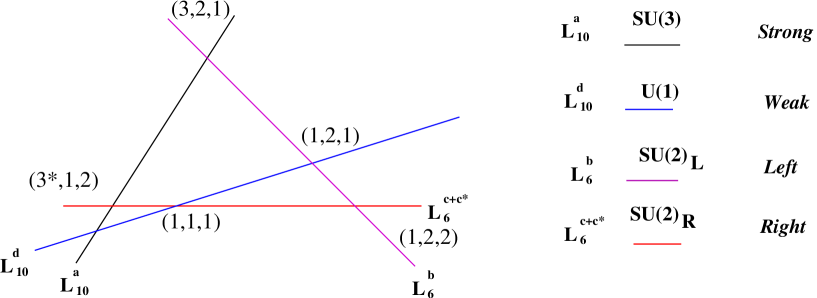
Figure 1: LR symmetric model obtained by orbifolding $6^{2}2$ $D=6$ model. Original ${\bf L_{10}},{\bf L_{6}}$ boundary states do split, under the action of the modding, into ${\bf L^{a}_{10}},{\bf L^{d}_{10}}$ and ${\bf L^{b}_{6}},{\bf L^{c}_{6}}$ branes, giving rise to LR spectrum at the intersection.

Besides states propagating between different branes we must consider states along the same type of branes. They lead to vector like matter.

Interestingly enough, massless states $(4020),(0420)$ and $(2220)$ do propagate in ${\bf L_{6}}-{\bf L_{6}}$ sector. They satisfy $\Gamma.\mu=\frac{1}{2}$ and thus, together with $(1)(0000)$, descending from the six dimensional vector, lead to

$$9(1,2,2)_{0}$$ (5.15)

candidates to LR Higgses. There is also a pair of states $(1,2,1)_{0}+(1,1,2)_{0}$ descending from the symmetric representation.

Notice that this sector is non chiral and that states fill up an ${\cal N}=2$ hypermultiplet

Branes $c$ and its image $c*$ are placed here on top of each other and on top of an orientifold point (leading to $Sp(2)$). Since such branes are parallel in the torus, following similar steps as discussed [31], we can think into separating them away from the orientifold point in the torus. Thus, $SU(2)_{R}\rightarrow U(1)_{c}$ where $U(1)_{c}$ charges are given by $T^{3}_{R}$ eigenvalues. Therfore, by introducing the weak hypercharge

$$Y=-T^{3}_{R}+\frac{1}{2}Q_{B-L}$$ (5.16)

we find that the original LR symmetric model breaks down to $SU(3)\times SU(2)_{L}\times U(1)_{Y}$ MSSM with three chiral generations

$$3[(3,2,1)_{\frac{1}{6}}+(\bar{3},1)_{-\frac{2}{3}}+(\bar{3},1)_{\frac{1}{3}}+(1,1)_{\frac{1}{2}}+(1,2)_{-\frac{1}{2}}+(1,1)_{0}]$$ (5.17)

including three right handed neutrini. Moreover, LR chiral states $(1,2,2)_{0}$ decompose into $(1,2)_{-1/2}+(1,2)_{1/2}$ with the correct MSSM Higgs charges.

A pictorial representation is presented in Figure 2.

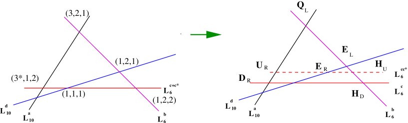
Figure 2: By separating ${\bf L^{c+c*}_{6}}\rightarrow{\bf L^{c}_{6}}+{\bf L^{c*}_{6}}$ away from the orientifold point breaking from LR to MSSM with 3 righthanded neutrini is achieved

Besides these basic boundary states leading to the MSSM structure, additional stacks of branes must be added in order to satisfy tadpole cancellation equations. Different choices are possible and each of them will give rise to particular phenomenological features. Here we just want to show a simple choice that allows to complete the above construction to a fully consistent supersymmetric model.

With this aim we introduce a stack of $N_{1}$ ${\bf L_{1}}$ “$N_{Z}$ branes” and three stacks of $N^{\prime}_{5}$ ${\bf L^{\prime}_{5}}$, $N^{\prime}_{1}$ ${\bf L^{\prime}_{1}}$, $N^{\prime}_{10}$ ${\bf L^{\prime}_{10}}$ “$D_{Z}$-branes”. Therefore the starting gauge group structure is

$$NN : SP(N_{6})\times U(N_{10})\times SP(N_{1})$$ (5.18)

$$DD : SP(N^{\prime}_{5})\times U(N^{\prime}_{10})\times SP(N^{\prime}_{1})$$ (5.19)

When performing the modding given in Eq.(5.1) tadpole equations (5.6) become

$$2N_{6}+2N_{10} = 16$$

$$N_{1}+3N_{6}+2N_{10} = 24$$

$$2Tr\gamma^{2}_{6}+2Tr\gamma^{2}_{10} = 0$$

$$Tr\gamma^{2}_{1}+3Tr\gamma^{2}_{6}+2Tr\gamma^{2}_{10} = 0$$

$$N^{\prime}_{5}+2N^{\prime}_{10} = 16$$

$$N^{\prime}_{1}+N^{\prime}_{5}+2N^{\prime}_{10} = 24$$

$$Tr{\gamma^{\prime}}^{2}_{5}+2Tr{\gamma^{\prime}}^{2}_{10} = 0$$

$$Tr{\gamma^{\prime 2}}_{1}+Tr{\gamma^{\prime}}^{2}_{5}+2Tr{\gamma^{\prime 2}}_{10} = 0$$

$$2Tr{\gamma}_{6}+2Tr{\gamma^{\prime}}_{5}+2(Tr{\gamma}_{10}+2Tr{\gamma^{\prime}}_{10}) = 0$$

$$Tr{\gamma}_{1}+2Tr{\gamma^{\prime}}_{1}+3Tr{\gamma}_{6}+2(Tr{\gamma}_{10}+2Tr{\gamma^{\prime}}_{10}) = 0$$

A solution is obtained by choosing $N_{1}=N_{6}=N_{10}=4$ in the DD sector and $N^{\prime}_{10}=1$, $N^{\prime}_{1}=8$, $N^{\prime}_{5}=14$ with the corresponding twists embedding (and induced gauge symmetry breaking) given in Table 5. Massless states propagating at intersection of different pairs of branes are shown in Table 6

Sector	Brane	twist	Group
NN	${\bf L_{10}}$	$V_{10}=\frac{1}{4}(1,1,1,3)$	$U(4)\rightarrow U(3)\times U(1)$
	${\bf L_{6}}$	$V_{6}=\frac{1}{4}(0,2)$	$Sp(4)\rightarrow SU(2)_{L}\times SU(2)_{R}$
	${\bf L_{1}}$	$V_{1}=\frac{1}{4}(1,1)$	$Sp(4)\rightarrow U(2)$
DD	${\bf L^{\prime}_{10}}$	$V^{\prime}_{10}=\frac{1}{4}(3)$	$U(1)$
	${\bf L^{\prime}_{1}}$	$V^{\prime}_{1}=\frac{1}{4}(0,2,1,1)$	$SP(8)\rightarrow SP(2)\times\times SP(2)\times U(2)$
	${\bf L^{\prime}_{5}}$	$V^{\prime}_{5}=\frac{1}{4}(0,0;2,2;1,1,1)$	$SP(14)\rightarrow SP(4)\times SP(4)\times U(3)$

Table 5: Original ${\bf L_{I}}$ branes do split due to twist $V_{I}$. The original gauge group living on ${\bf L_{I}}$ world volume breaks accordingly.

Sector	Branes	States	IRREP
NN	${\bf L_{10}}-{\bf L_{6}}$	$(3310)$, $(5110)$,$(1510)$	SM
N	${\bf L_{10}}-{\bf L_{1}}$	$(3310)$	none
ND	${\bf L_{10}}-{\bf L^{\prime}_{1}}$	$(3310)$	$(3,1,1;2,1,1)_{1/3}+(1,1,1;2,1,1)_{-1/3}+$
			$(3,1,1;1,2,1)_{-1/3}+(1,1,1;1,2,1)_{1/3}$
ND	${\bf L_{10}}-{\bf L^{\prime}_{5}}$	$(3310)$	$(3,1,1;4,1,1)_{1/3}+(1,1,1;4,1,1)_{-1/3}+$
			$(3,1,1;1,4,1)_{-1/3}+(1,1,1;1,4,1)_{1/3}$
NN	${\bf L_{6}}-{\bf L_{1}}$	$(4400)+(2200)$	none
ND	${\bf L_{6}}-{\bf L^{\prime}_{1}}$	$(4400)+(2200)$	$(1,{\underline{2,1}};{\underline{2,1}},1)_{0}$
ND	${\bf L_{6}}-{\bf L^{\prime}_{10}}$	$(3310),(5110),(1510)$	none
ND	${\bf L_{6}}-{\bf L^{\prime}_{5}}$	$(6200),(4400),(2220),(0420)$,	$(1,{\underline{2,1}};{\underline{4,1}},1)_{0}$
ND	${\bf L_{1}}-{\bf L^{\prime}_{10}}$	$(3310)$	3(1,2,1;1)+3(1,1,2;1)
ND	${\bf L_{1}}-{\bf L^{\prime}_{5}}$	$(2600),(4020)$	$(2,1,3,1)+({\bar{2}},1,{\bar{3}},1)$
			$(2,1,{\bar{3}},1)+({\bar{2}},1,{3},1)$
DD	${\bf L^{\prime}_{10}}-{\bf L^{\prime}_{1}}$	$(3310)$	$(1;2,1,1)+(1;1,1,2)$
DD	${\bf L^{\prime}_{10}}-{\bf L^{\prime}_{5}}$	$(3310)$	$(1,1,1;4,1,1)+(1,1,1;1,4,1)$

Table 6: Massless chiral primary states, denoted by $(m_{1},\dots,m_{6})$ propagating between a pair of branes ${\bf L_{I}}-{\bf L_{J}}$ are indicated. After performing the orbifold twist, the original gauge group in each brane breaks into several subgroups as in Table 5 above. The last column shows the representations, with respect to such subgroups, in which chiral superfields accommodate.

A study of interactions among LR states and extra matter is beyond the scope of the present work. Nevertheless, some general remarks about Yukawa couplings can be advanced.

As a general observation notice that a Yukawa coupling will have the form

$$Y_{ijk}\Phi^{i}_{ba}\Phi^{j}_{ac}\Phi^{k}_{cb}$$ (5.20)

where $\Phi_{ab}$ is the chiral superfield insertion connecting boundaries $a$ and $b$ and $i,j,k$ refers to internal CFT labels. Such a term should be a singlet of the gauge group and invariant under $\Gamma$ modding. Moreover, it must be allowed by the fusion rules (C) of the internal conformal field theory [35, 30]. Namely,

$$Y_{ijk}\propto\langle ijk\rangle\propto{\cal N}_{ij}^{k}$$ (5.21)

For instance, couplings like

$$[({\underline{51}}10)](3,2,1)_{1/3}^{ab}\times[(3310))]({\bar{3}},1,2)_{-1/3}^{ac}[(2220)](1,2,2)_{0}^{bc}\$$ (5.22)

(where we have indicated the internal charges in brackets) are non vanishing and lead to degenerate masses for two quark generations. Fusion rules forbid masses for the first quark generation (see (5)). A similar result is obtained for lepton masses since the same internal states are involved for leptonic Yuakawa couplings.

The general pattern is very similar (the number of Higgses is different) to the one found in Ref.[36] in the context of branes at singularities.

It is interesting to notice that couplings of quarks or leptons to states $[({\underline{40}}20)](1,2,2)_{0}$ and $[(1)(0000)](1,2,2)_{0}$, discussed in (5.15), are not allowed by fusion rules. Thus, the model contains four effective LR Higgses.

In particular, as addressed in in [36], the full picture of mass structures becomes more complicated due, for instance, to the presence of Yukawa couplings of quarks with colored triplets present at other intersections. For instance, D quarks will couple to triplets in the ${\bf L_{10}}-{\bf L^{\prime}_{1}}$ sector

$$[(3310))]({\bar{3}},1,2)_{-1/3}^{ac}\times[(3310))]({3},1,1;2,1,1)_{1/3}^{a1^{\prime}}\times[(2200)](1,1,2;2,1,1)_{0}^{1^{\prime}c}\$$ (5.23)

and therefore D quarks and triplets mix once $SU(2)_{R}$ doublet acquires a vev. Through similar terms all the three quarks would become massive.

Notice also that, from the 9 candidates to be interpreted as Higgs particles coming from ${\bf L_{6}}-{\bf L_{6}}$ sector, only those with CFT quantum numbers $(2220)$ are allowed in Yukawa couplings. For all of them, on the other hand, mass term like couplings are allowed. Thus, we can imagine a scenario where some of the $(1,2,2)$ multiplets become very massive.

5.0.1 An alternative with the LR week sector on DD branes

In the example discussed above the basic branes ${\bf L_{10}}$, containing strong group, and ${\bf L_{6}}$, where $SU(2)_{L}\times SU(2)_{R}$ lives, were placed in the same NN sector. However, it might be useful for future phenomenological applications, to place the part of the spectrum containing the $SU(2)_{L}\times SU(2)_{R}$ gauge theory on the branes in the DD sector.

An interesting possibility of this kind is shown in Table 7. In this case, even if ${\bf L_{6}}$ is placed in DD sector, tadpole cancellation requires to place a similar stack in NN sector thus leading to two alternatives realizations of (3 generations) LR models. Extra boundary states, required by consistency, are of the same kind we introduced in previous example, thus, states propagating between different pairs of branes can read directly from third column in Table [6].

Sector	Brane	twist	Group
NN	${\bf L_{10}}$	$V_{10}=\frac{1}{4}(1,1,1,3)$	$U(4)\rightarrow U(3)\times U(1)$
	${\bf L_{6}}$	$V_{6}=\frac{1}{4}(0,2)$	$Sp(4)\rightarrow SU(2)_{L}\times SU(2)_{R}$
	${\bf L_{1}}$	$V_{1}=\frac{1}{4}(1,1)$	$Sp(4)\rightarrow U(2)$
DD	${\bf L^{\prime}_{10}}$	$V^{\prime}_{10}=\frac{1}{4}(3)$	$U(1)$
	${\bf L^{\prime}_{6}}$	$V^{\prime}_{6}=\frac{1}{4}(0,2)$	$Sp(4)\rightarrow SU(2)_{L}\times SU(2)_{R}$
	${\bf L^{\prime}_{1}}$	$V^{\prime}_{1}=\frac{1}{4}(1,1)$	$Sp(4)\rightarrow U(2)$
	${\bf L^{\prime}_{5}}$	$V^{\prime}_{5}=\frac{1}{4}(1,1,1)$	$SP(6)\rightarrow U(3)$

Table 7: An alternative construction leading to a duplicated LR structure. The group $SU(2)_{L}\times SU(2)_{R}$ can be chosen to be in the DD sector or in the NN sector.

It can be easily verified that this solution satisfies tadpole equations.

5.0.2 Massless U(1) and K-theory constraints

Anomalous $U(1)$ generators acquire mass through the Green-Schwarz mechanism. However, a non-anomalous U(1) may also become massive if there is an effective coupling $B\wedge F$. We must therefore ensure that $Q_{B-L}$ is not one of them and remains massless.

For a $U(1)_{a}$ gauge group on a brane $a$, we will have the coupling

$$\int_{[M_{4}]}(C_{2}^{a}-{C_{2}^{a}}^{\prime})\wedge F^{a}$$ (5.24)

where, in a geometrical setting, $C_{2}^{a}$ (${C_{2}^{a}}^{\prime}$ is its $\Omega$-image) come from the reduction of a $C_{p}$ form on a supersymmetric cycle $a$ and $F_{a}$ is the $U(1)_{a}$ gauge field.

Therefore, by expanding $C_{2}^{a}$ forms, or analogously their corresponding cycles, into Ishibashi states, with expansion coefficients $D_{a}^{i}$ (and their $\Omega$-images ${D^{\prime}}_{a}^{i}$) ([9]), and requiring $Q_{B-L}=\sum x_{a}Q^{a}$ coupling to vanish leads to

$$N_{a}(D_{a}^{i}-{D_{a}^{i}}^{\prime})x_{a}=0$$ (5.25)

for each Ishibashi state $|i\rangle\rangle=|\lambda\mu;x\rangle\rangle$ in the orbifold theory.

For the Ishibashi state $I=|(33)(33)(11)(00)^{3};x=1\rangle\rangle$ we obtain

$$3x_{a}i(D_{10,+}^{I}-D_{10,-}^{I})-x_{d}i(D_{10,+}^{I}-D_{10,-}^{I})=0$$ (5.26)

where $D_{10,\pm}$ are the expansion coefficients for the parts $a$ or $d$ of the brane ${\bf L_{10}}$ (4.4) in terms of Ishibashi states.

Then a solution with $x_{a}=1/3$ and $x_{d}=1$ corresponds to having

$$Q_{B-L}=\frac{1}{3}Q_{3}+Q$$ (5.27)

massless . It can be shown that this is the only nontrivial condition.

Finally, there are additional constraints on the compactified theory coming from the fact that D-brane charges are classified by K-theory [48]. One particular constraint is the vanishing of the Witten global anomaly which means that the number of massless fermions in the fundamental representation of a symplectic group is even. We have verified that the Witten anomaly vanishes in the example we presented in the last section.

Generically, however, K-theory might impose additional constraints. It would be interesting to further check consistency using maybe the method of probe-branes where additional constraints might appear  [49].

6 Summary and outlook

In the first part of the present work we have addressed the construction of six dimensional Type IIB orientifold models based on a Gepner models internal space

Six dimensional models were constructed by considering stacks of B-type boundary states, required by a diagonal invariant partition function. Such boundary states would correspond to D branes wrapping even cycles of $K3$ [38, 24]. We have found the explicit expressions for these boundary states and the rules to compute their massless states spectra (associated to open strings propagating among them). Tadpole cancellation equations were also derived. Explicit computations for the sixteen diagonal Gepner models present in $D=6$ will be collected in [21].

We have also shown how moddings by internal discrete symmetries and the so called parity and quantum dressings can be included in this context. In particular, A-type boundary models, corresponding to a charge conjugation invariant, should be obtainable [29] by performing possible moddings on B-type construction.

As shown in Ref.[38, 24], more general boundary states, corresponding $SO(3)$ rotations, and including A and B-type cases, can be constructed in $K3$. It would be interesting to explore how such states could be obtained in the present context

Following the ideas presented in Ref.[1], four dimensional chiral models were built by further compactifying on a $T^{2}$ torus, sharing some of the symmetries of the $D=6$ models, and by modding out by such symmetries. The projection is realized as the combined action of a phase symmetry modding of the Gepner sector and a rotation of the torus lattice accompanied by a twist on Chan-Paton factors. The twist on Chan Paton factors can be viewed as a breaking of the original boundary states into component states with specific monodromy under the twist. Generically, when even order moddings are considered, new sets of branes are required for tadpole cancellation.

Interestingly enough, inspection of six dimensional spectra allows to identify phenomenologically appealing models without the use of a computer scanning.

As an example of the construction, we described a $Z_{4}$ modding of the model $6620\times\bf T^{2}$. In such a model a basic structure of two stacks of four boundary states , which we call ${\bf L}_{10}$ and ${\bf L}_{6}$, exist, with gauge groups $U(4)$ and $Sp(4)$ respectively, living on their world volumes with three hypermultiplets propagating between them. These two stacks of boundary states constitute the basic, six dimensional, “bulding blocks” of the MSSM. In fact, we showed that further compactification on a torus, accompanied by $Z_{4}$ modding, leads to the breaking

$${\bf L_{10}}[\,U(4)] \rightarrow {\bf L^{a}_{10}}[\,U(3)]+{\bf L^{d}_{10}}[\,U(1)]$$

$${\bf L_{6}}[\,Sp(4)] \rightarrow {\bf L^{b}_{6}}[\,Sp(2)]+{\bf L^{c}_{6}}[\,Sp(2)]$$

namely, into a four stacks of branes, giving rise to a Left-Right symmetric model with three massless generations living at the boundary states intersections. Further breaking to a MSSM (with the expected three right handed neutrinos) can be achieved.

The four stacks $a,b,c,d$ of boundary states, possess the “basic building block” properties used in intersecting brane realizations [18, 39] of the Standard Model. They can be further embedded into a fully consistent supersymmetric orientifold model.

We have indicated in the example some appealing features of the basic Yuakawa couplings structure. For instance, the fact that vertex operators must connect different boundary states, the requirement of gauge and discrete twist invariance and the CFT fusion rules allow to discard several terms. A detailed investigation of the structure of Yuakawa couplings remains to be done. In particular, it would be interesting to see if a more systematic study, like in [31] for intersecting branes, can be pursued in this context of RCFT.

An interesting feature of the hybrid construction is that lowering of the string scale [40, 41, 18, 42, 43, 39] could be achieved by considering large extra dimensions in the $T^{2}$ torus, transverse to the whole configuration of intersecting boundary states.

Indeed, in the present examples of the type $Gepner\times T^{2}/\bf Z_{N}$, boundary states would correspond to branes wrapping cycles on $K_{3}$ and stuck at a ${\bf C/\bf Z_{N}}$ singularity. Thus, if we denote by $V_{4}$ the volume of the Gepner piece, which should be of the order of the string scale $V_{4}\propto 1/M_{s}^{4}$, and by $V_{2}$ that of two dimensional manifold. Then we expect the Planck scale, after dimensional reduction to four dimensions, to be

$$M_{Planck}\ =\ \frac{2}{\lambda}M_{s}^{4}\sqrt{V_{4}V_{2}}$$ (6.1)

where $\lambda$ is the string coupling. Therefore the string scale $M_{s}$ can be lowered by choosing the volume $V_{2}$ ($V_{2}\ =\ \frac{M_{Planck}^{2}\lambda^{2}}{4M_{s}^{4}}$) sufficiently large. Recall that the models constructed here are fully supersymmetric and though lowering the scale could be phenomenologically attractive in some cases it is not as compelling as in non supersymmetric models.

Presumably, having these large extra dimension could allow for the introduction of dilute fluxes in a supergravity limit of some of these hybrid construction  [50].

Acknowledgments

We are grateful to A. Font, L.E. Ibañez and A. Uranga for stimulating observations and suggestions. G.A. work is partially supported by ANPCyT grant PICT 11064 and CONICET PIP. J. J. is grateful to the Particle and Field Group of the Bariloche Atomic Center (CAB) for partial support and hospitality during the first part of this work.

Appendix A SO(2d) Space- time partition functions

We show the basic ingredients needed for the computation of modular transformation matrices of the space- time part of the partition functions of closed and open sectors. Even if we are mainly interested in $D=6$ dimensions we present here the general result in $D$ dimensions Consider $SO(2d)$ $d=\frac{D-2}{2}$ for dimensions $D=4,6,8$. There exist four representations $\Lambda>=|0>,|v>,|s>,|c>$ whose fundamental weights are encoded as

$$|0> = (0,0,\dots,0)$$ (A.1)

$$|v> = (1,0,\dots,0)$$

$$|s> = (\frac{1}{2},\frac{1}{2},,\dots,\frac{1}{2})$$

$$|c> = (\frac{1}{2},\frac{1}{2},,\dots,-\frac{1}{2})$$

Scalar product between two representations $\Lambda$ and $\Lambda^{\prime}$ is given by

$$\Lambda.\Lambda^{\prime}=\sum_{l=0}^{d-1}\Lambda_{l}\Lambda_{l}$$ (A.2)

Recall that we need to redefine $\Lambda_{Gepner}=2\Lambda$ in order to have the normalization usually used in Gepner models.

The character that is associated to highest weight $\Lambda$, at level one, is given by $\chi_{\Lambda,1}(\tau)=\theta_{\Lambda,1}(\tau)$ [47]. It leads to modular transformation matrices

$$S_{\Lambda,\Lambda^{\prime}} = e^{-2i\pi\Lambda.\Lambda^{\prime}}$$ (A.3)

$$T_{\Lambda,\Lambda^{\prime}} = e^{2i\pi(\Lambda^{2}-\frac{d}{24})}\delta({\Lambda,\Lambda^{\prime}})$$ (A.4)

Therefore, the space time matrix $P$ [28] can be obtained as

$$\hat{P}_{\Lambda,\Lambda^{\prime}}=T_{\Lambda}^{\frac{1}{2}}S_{\Lambda,\Lambda^{\prime\prime}}T_{\Lambda^{\prime\prime},\Lambda^{\prime\prime}}^{2}S_{\Lambda^{\prime\prime},\Lambda}T_{\Lambda^{\prime\prime}}^{\frac{1}{2}}$$ (A.5)

where $T_{\Lambda}^{\frac{1}{2}}=e^{i\pi(h_{\Lambda}-\frac{d}{24})}$ is the phase factor that is introduced in order to construct a real character from $\theta_{\Lambda,1}(\tau+\frac{1}{2})$ and $h_{\Lambda}$ is the conformal weight. It coincides with $\Delta=\frac{\Lambda^{2}}{2}$ only in the case in which quantum numbers $\Lambda$ are given in the standard range above. Thus, $P$ reads

$${\hat{P}}_{\Lambda,\Lambda^{\prime}}=e^{-i\pi\frac{d}{4}}e^{i\pi(h_{\Lambda}+h_{\Lambda^{\prime}})}\sum_{\Lambda^{\prime\prime}}e^{-2i\pi\Lambda.\Lambda^{\prime\prime}}e^{2i\pi(\Lambda^{\prime\prime})^{2}}e^{-2i\pi\Lambda^{\prime\prime}.\Lambda^{\prime}}$$ (A.6)

It is easy to see that, when all states are in the range above, the matrix $P$ is given by

$${P}=\left(\begin{array}[]{cccc}c&s&0&0\\ s&-c&0&0\\ 0&0&\zeta c&i\zeta s\\ 0&0&i\zeta s&\zeta c\end{array}\right)$$ (A.7)

with $c=cos\pi d/4$ and $s=sin\pi d/4$.

Since in the actual computation of Möbius amplitude weights are shifted from the standard range by $\beta_{i},\beta_{0}$ vectors, it appears useful to rewrite $P$ as (see for instance ([5] for $d=1$))

$${\hat{P}}_{\Lambda,\Lambda^{\prime}}=\sigma(\Lambda)\sigma(\Lambda^{\prime})e^{-i\pi\frac{d}{4}}e^{-i\pi{\Lambda\Lambda^{\prime}}}\sum_{\Lambda^{\prime\prime}}e^{2i\pi(\Lambda^{\prime\prime}-\frac{\Lambda+\Lambda^{\prime}}{2})^{2}}$$ (A.8)

where

$$\sigma(\Lambda)=(-1)^{(\frac{\Lambda^{2}}{2}-h_{\Lambda})}$$ (A.9)

and

$${\tilde{P}}_{\Lambda,\Lambda^{\prime}}=\sum_{\Lambda^{\prime\prime}}e^{2i\pi(\Lambda^{\prime\prime}-\frac{\Lambda+\Lambda^{\prime}}{2})^{2}}$$ (A.10)

which, for NS weights (scalar or vector) reads

$${\tilde{P}_{(\Lambda_{0}+\Lambda^{\prime}_{0}+\nu_{i}\beta_{i})}^{NS}}=\left\{\begin{array}[]{lll}&1&d=1\\ &-e^{i\pi(\Lambda_{0}+\Lambda^{\prime}_{0}+\sum\nu_{i})}&d=3\\ &\frac{1}{2}(1-e^{i\pi(\Lambda_{0}+\Lambda^{\prime}_{0}+\sum\nu_{i})}&d=2\end{array}\right.$$

Appendix B The crosscap state in D=6

The $D=6$ spacetime bosons and fermions realize a $(2,2)$ superconformal algebra. The four world-sheet fermions $\psi^{2,3,4,5}$ have an $SO(4)$ symmetry which requires them to be organized into unitary representations of the affine transverse Lorentz algebra at level $k=1$. These are the scalar, vector, spinor and conjugate spinor representations labelled respectively by $s_{0}=-1,0,1,2$. It proves convenient to split the representations of $SO(4)$ at level $1$ into those of $SO(2)\times SO(2)$. The latter are labelled by two numbers $\Lambda_{0},\Lambda_{1}=-1,0,1,2$ subject to $\Lambda_{0}+\Lambda_{1}=0\mod{2\mathbf{Z}}$.

In order to implement a GSO projection we define the vectors $\mu$’s and the inner product between them as

$$\lambda=(l_{1},\dots,l_{r})$$

$$\mu=(\Lambda_{0},\Lambda_{1};s_{1},\dots,s_{r};m_{1},\dots,m_{r}),$$

$$\mu\bullet\mu^{\prime}\equiv-\frac{\Lambda_{0}\Lambda_{0}^{\prime}}{4}-\frac{\Lambda_{1}\Lambda_{1}^{\prime}}{4}-\sum_{j}\frac{s_{j}s_{j}^{\prime}}{4}+\sum_{j}\frac{m_{j}m_{j}^{\prime}}{2(k_{j}+2)}.$$

It is convenient to introduce special vectors $\beta_{0}$, $\beta_{j}$ and $\tilde{\beta}_{1}$

$$\beta_{0}=(1,1;1,\dots,1;1,\dots,1),$$

$$\beta_{j}=(0,2;0,\dots,0,\underset{j}{2},0,\dots,0;0,\dots,0),\ (j=1,\dots,r),$$

$$\tilde{\beta}_{1}=(2,2;0,\dots,0;0,\dots,0).$$

By using these vectors, we can construct the building blocks $\chi^{\lambda}_{\mu}(\tau)$ as

$$\chi^{\lambda}_{\mu}(\tau)=\chi_{\Lambda_{0}}(\tau)\chi_{\Lambda_{1}}(\tau)\chi_{m_{1}s_{1}}^{l_{1}}(\tau)\dots\chi_{m_{r}s_{r}}^{l_{r}}(\tau)$$

where $\chi_{\Lambda_{0}}(\tau)$ and $\chi_{\Lambda_{1}}(\tau)$ are $\widehat{SO(2)}_{1}$ characters. Then the GSO conditions and the condition of fermionic sectors are

$$2\beta_{0}\bullet\mu\in 2\mathbf{Z}+1,\qquad\beta_{j}\bullet\mu\in\mathbf{Z},\qquad\tilde{\beta}_{1}\bullet\mu\in\mathrm{Z},$$ (B.1)

The type-B, GSO-projected partition function is then given by

$$Z_{D}^{B}(\tau,\overline{\tau})=\frac{1}{2^{r}}\frac{({\rm Im}\tau)^{-3}}{|\eta(q)|^{6}}\sum_{b_{0}=0}^{K-1}\sum_{\tilde{b}_{1},b_{1},\ldots,b_{r}=0}^{1}{\sum_{\lambda,\mu}}^{\beta}(-1)^{s_{0}}\ \chi^{\lambda}_{\mu}(q)\,\chi^{\lambda}_{\mu+b_{0}\beta_{0}+\tilde{b}_{1}\tilde{\beta}_{1}+b_{1}\beta_{1}+\ldots b_{r}\,\beta_{r}}(\overline{q}).$$ (B.2)

Here $K={\rm lcm}(4,2k_{j}+4)$ and ${\sum}^{\beta}$ means that the sum is restricted to those $\lambda$ and $\mu$ satisfying (B.1).

The Klein bottle partition function is obtained from that of the torus by keeping states with equal left and right oscillators. In the direct channel it is given by

$$Z_{K}^{B} = {\frac{4}{(4\pi^{2}\alpha^{\prime})^{3}}}\int_{0}^{\infty}{\frac{dt}{4t^{4}}}{\rm Tr^{\prime}}_{cl}\left({\frac{\Omega}{2}}e^{-4\pi t\left(L_{0}-{\frac{c}{24}}\right)}\right)$$ (B.3)

where ${\rm Tr^{\prime}}_{cl}$ denotes the trace over the oscillator modes in the closed string sector. The integration over the bosonic zero modes yields the factor $(4\pi^{2}\alpha^{\prime})^{3}$.

The Klein bottle amplitude in the transverse channel is obtained by performing an $S$ modular transformation

$$\widetilde{Z}_{K}^{B} = 2^{7}\prod_{j}\frac{\sqrt{k_{j}+2}}{2^{\frac{3r}{2}}K}\,\int_{0}^{\infty}{dl}\,\frac{1}{\eta(2il)^{3}}{\sum_{\lambda^{\prime},\mu^{\prime}}}^{ev}\sum_{\nu_{0}=0}^{K-1}\sum_{\nu_{1},\ldots,\nu_{r}=0}^{1}\sum_{\epsilon_{1},\ldots,\epsilon_{r}=0}^{1}\sum_{\eta_{1},\ldots,\eta_{r}=0}^{1}$$

$$(-1)^{\nu_{0}}\,\delta_{\Lambda_{0}^{\prime},2+\nu_{0}+2\sum\nu_{j}}^{(4)}\delta_{\Lambda_{1}^{\prime},\nu_{0}}^{(4)}$$

$$\prod_{j=1}^{r}\Biggl{(}\frac{P_{l^{\prime}_{j},\epsilon_{j}k_{j}}P_{l^{\prime}_{j},(\epsilon_{j}+\eta_{j})k_{j}}}{S_{l^{\prime}_{j},0}}\,\delta_{m_{j}^{\prime},\nu_{0}+(1-\epsilon_{j})(k_{j}+2)}^{(2k_{j}+4)}\,\delta_{s_{j}^{\prime},\nu_{0}+2\nu_{j}+2(1-\epsilon_{j})}^{(4)}\Biggr{)}\,\chi^{\lambda^{\prime}}_{\mu^{\prime}}(2il)$$

where $l=1/t$.

From the Klein bottle amplitude in the transverse channel we can read the expression for the crosscap state up to signs which are contained in the Möbius strip amplitude. The result is that the crosscap state is given by

$$|C\rangle^{NS}_{B} = \frac{1}{\kappa_{c}}{\sum_{\lambda^{\prime},\mu^{\prime}}}^{ev}\sum_{\nu_{0}=0}^{\frac{K}{2}-1}\sum_{\nu_{1},\ldots,\nu_{r}=0}^{1}\sum_{\epsilon_{1},\ldots,\epsilon_{r}=0}^{1}\,\,$$

$$\eta(\nu_{0},\nu_{i},\epsilon_{j})\delta_{\Lambda^{\prime}_{0},2+2\nu_{0}+2\sum\nu_{j}}^{(4)}\delta_{\Lambda^{\prime}_{1},2\nu_{0}}^{(4)}$$

$$\prod_{j=1}^{r}\Biggl{(}\frac{P_{l^{\prime}_{j},\epsilon_{j}k_{j}}}{\sqrt{S_{l^{\prime}_{j},0}}}\,\delta_{m_{j}^{\prime},2\nu_{0}+(1-\epsilon_{j}+\omega_{j})(k_{j}+2)}^{(2k_{j}+4)}\delta_{s_{j}^{\prime},2\nu_{0}+2\nu_{j}+2(1-\epsilon_{j})}^{(4)}\Biggr{)}|\lambda^{\prime},\mu^{\prime}\rangle\rangle_{c}$$

We still have to fix the signs of the crosscap state. As in [5], the condition that GSO orbits of hatted characters transforms,under the $P$-transformation, into themselves will be used as an ansatz to fix the signs in the crosscap state.

We want to compute the modular transformation of

$${M^{\lambda}_{\mu}=\sum_{\nu_{0}=0}^{\frac{K}{2}-1}\sum_{\nu_{1},\ldots,\nu_{r}=0}^{1}(-1)^{\left[h^{\lambda}_{\mu}(\nu_{0},\nu_{j})-h^{\lambda}_{\mu}\right]}\,\,\widehat{\chi}^{\lambda}_{\mu+2\nu_{0}\beta_{0}+\sum\nu_{j}\beta_{j}}(it+{\textstyle{\frac{1}{2}}}),}$$ (B.6)

Thus, when we perform the $P$ transformation in (B.6) we get

$$M^{\lambda}_{\mu} = \sum_{\mu^{\prime},\lambda^{\prime}}^{\beta}\sum_{\nu_{1},\ldots,\nu_{r}=0}^{1}\prod_{k<l}(-1)^{\nu_{l}\nu_{k}}\sigma^{\prime}_{(l^{\prime},m^{\prime},s^{\prime})}e^{i\pi\sum\nu_{i}(\Lambda_{0}+s_{i}-\Lambda^{\prime}_{0}-s^{\prime}_{i}+1)}e^{-i\pi{\mu.\mu^{\prime}}}\delta_{s_{i}+s_{i}^{\prime},0}^{(1)}$$ (B.7)

$$\tilde{P}_{(\Lambda_{0}+\Lambda^{\prime}_{0}+\nu_{i}\beta_{i})}\sum_{\epsilon=0}^{1}P_{l,|\epsilon k-l^{\prime}|}\,\delta_{m+m^{\prime}+(1-\epsilon)(k+2)}^{(2)}$$

$$(-1)^{\epsilon_{i}(\frac{l_{i}^{\prime}+m_{i}^{\prime}}{2}+s_{i}^{\prime})}(-1)^{\epsilon_{i}(\frac{m_{i}}{2}+s_{i}+\nu_{i})}\,\,\widehat{\chi}^{\lambda}_{\mu^{\prime}}(it+\frac{1}{2})$$

where the spacetime $\tilde{P}$-matrix is given in (A.10) for $d=2$.

By summing over $\nu_{i}$ we are lead to

$$M^{\lambda}_{\mu} = \sum_{\mu^{\prime},\lambda^{\prime}}^{\beta}\sum_{\nu_{1},\ldots,\nu_{r}=0}^{1}\sigma^{\prime}_{(l^{\prime},m^{\prime},s^{\prime})}$$ (B.8)

$$\prod_{k<l}(-1)^{\eta_{l}\eta_{k}}\delta^{(2)}_{\Lambda_{0}+\Lambda_{1}+\Lambda^{\prime}_{0}+\Lambda^{\prime}_{1}+\sum\nu_{i},0}e^{-i\pi{\mu.\mu^{\prime}}}\delta_{s_{i}+s_{i}^{\prime},0}^{(1)}$$

$$\sum_{\epsilon=0}^{1}P_{l_{i},|\epsilon k_{i}-l_{i}^{\prime}|}\,\delta_{m_{i}+m_{i}^{\prime}+(1-\epsilon_{i})(k_{i}+2)}^{(2)}$$

$$(-1)^{\epsilon_{i}(\frac{l_{i}^{\prime}+m_{i}^{\prime}}{2}+s_{i}^{\prime})}(-1)^{\epsilon_{i}(\frac{m_{i}}{2}+s_{i})}\,\,\widehat{\chi}^{\lambda}_{\mu^{\prime}}(it+\frac{1}{2})$$

$$\eta_{i}=\Lambda_{0}+s_{i}-\Lambda^{\prime}_{0}-s^{\prime}_{i}+1+\epsilon_{i}$$ (B.9)

Using (B.8) we determine the unknown signs $\eta(\nu_{0},\nu_{i})$ in (B) to obtain the expression (3), for the crosscap state.

Appendix C MS amplitude in the direct channel

We present here the expression for the tree-channel Möbius amplitude required to extract the gauge and matter field content. It can be computed from the amplitude of closed strings propagating between a boundary state (3) and the crosscap state (3) and then performing a modular transformation to open string channel.

$${{\cal Z}_{M}}^{B,NS}_{\alpha} = \langle C|q^{H}|{\alpha}\rangle_{B}=$$

$$= -\frac{1}{2^{r+1}}\int_{0}^{\infty}\frac{dt}{t^{5}}\,\frac{1}{\eta(it+\frac{1}{2})^{3}}{\sum_{\lambda,\mu}}^{ev}\sum_{\epsilon_{1},\ldots,\epsilon_{r}=0}^{1}\left(\prod_{k<l}(-1)^{\rho_{k}\rho_{l}}\right)$$

$$e^{i(\pi/2)\sum\omega_{j}(m_{j}-2L_{j}+\epsilon_{j}(k_{j}+2))}(-1)^{\sum\omega_{j}\Lambda_{0}/2}$$

$$\delta_{\sum_{j}\rho_{j},1+\frac{\Lambda_{0}+\Lambda_{1}}{2}+\sum\omega_{j}}^{(2)}\,\delta_{\Lambda_{0},0}^{(2)}\delta_{\Lambda_{1},0}^{(2)}\delta_{\sum\frac{K^{\prime}}{2k_{j}+4}\left[2(M_{j}-\Delta_{j})-m_{j}-\epsilon_{j}(k_{j}+2)\right],0}^{(K^{\prime})}$$

$$\,\prod_{j=1}^{r}\Biggl{(}\sigma_{(l_{j},m_{j},s_{j})}\,\,Y_{L_{j},\epsilon_{j}\,k_{j}}^{l_{j}}\,\,\delta_{m_{j}+\epsilon_{j}(k_{j}+2),0}^{(2)}$$

$$\delta_{s_{j},0}^{(2)}\,(-1)^{\frac{\epsilon_{j}}{2}\left[2S_{j}-s_{j}-2\epsilon_{j}\right]}\,(-1)^{\frac{(1-\epsilon_{j})}{2}\left[2M_{j}-m_{j}-\epsilon_{j}(k_{j}+2)\right]}\Biggr{)}$$

$$\,\widehat{\chi}^{\lambda}_{\mu}(it+{\textstyle\frac{1}{2}})$$

where $\rho_{j}=\frac{\Lambda_{0}+s_{j}}{2}+\epsilon_{j}-1+\sum\omega_{j}$.

Here

$$Y_{l_{1},l_{2}}^{l_{3}}=\sum_{l=0}^{k}\frac{S_{l_{1},l}\,P_{l_{2},l}\,P_{l_{3},l}}{S_{0,l}}=(-1)^{\frac{1-\epsilon_{j}}{2}(2L_{j}+lj)}N_{L_{j},L_{j}}^{|\epsilon_{j}k_{j}-l_{j}|}$$ (C.2)

in terms $SU(2)_{k}$ fusion coefficients [34]

$$N_{L_{1},L_{2}}^{l}=\left\{\begin{array}[]{lll}&&1\quad{\rm if}\quad|L_{1}-L_{2}|\leq l\leq{\rm min}\{{L_{1}+L_{2},2k-(L_{1}+L_{2})}\}\\ &&L_{1}+L_{2}+l=\,{\rm even}\\ &&N_{L_{1},L_{2}}^{l}=0\,\quad{\rm otherwise}\end{array}\right.$$

References

- [1] G. Aldazabal, E. C. Andrés and J. E. Juknevich, Particle models from orientifolds at Gepner-orbifold points, JHEP 0405, 054 (2004), hep-th/0403262.
- [2] R. Blumenhagen and A. Wisskirchen, Spectra of 4D, N = 1 type I string vacua on non-toroidal CY threefolds, Phys. Lett. B438 (1998) 52, hep-th/9806131.
- [3] S. Govindarajan and J. Majumder, Crosscaps in Gepner models and type IIA orientifolds, JHEP 0402 (2004) 026, hep-th/0306257.
- [4] G. Aldazabal, E. C. Andrés, M. Lestón and C. Nuñez,Type IIB orientifolds on Gepner points JHEP 0309, 067 (2003), hep-th/0307183.
- [5] R. Blumenhagen, Supersymmetric orientifolds of Gepner models JHEP 0311, 055 (2003), hep-th/0310244.
- [6] R. Blumenhagen and T. Weigand, Chiral supersymmetric Gepner model orientifolds, JHEP 0402 (2004) 041, hep-th/0401148.
- [7] I. Brunner, K. Hori, K. Hosomichi and J. Walcher,Orientifolds of Gepner models, hep-th/0401137.
- [8] R. Blumenhagen and T. Weigand, A Note on Partition Function of Gepner Model Orientifolds Phys.Lett. B591 (2004) 161-169, hep-th/0403299.
- [9] T. P. T. Dijkstra, L. R. Huiszoon and A. N. Schellekens, Chiral supersymmetric standard model spectra from orientifolds of Gepner models, Phys. Lett. B 609, 408 (2005), hep-th/0403196.
- [10] T.P.T. Dijkstra, L.R. Huiszoon, A.N. Schellekens, Supersymmetric Standard Model Spectra from RCFT Orientifolds , Nucl.Phys.B710:3-57,2005, hep-th/0411129.
- [11] C. Angelantonj, M. Bianchi, G. Pradisi, A. Sagnotti and Y. Stanev, Comments on Gepner models and Type I vacua in string theory, Phys. Lett. B387 (1996) 743, hep-th/960722.
- [12] D. Gepner, Lectures On N=2 String Theory, Lectures at Spring School on Superstrings, Trieste, Italy, Apr 3-14, 1989.
- [13] J. Fuchs, A. Klemm, C. Scheich and M. G. Schmidt, Spectra And Symmetries Of Gepner Models Compared To Calabi-Yau Compactifications, Annals Phys. 204, 1 (1990).
- [14] J. Fuchs, A. Klemm, C. Scheich and M. G. Schmidt, Gepner Models With Arbitrary Affine Invariants And The Associated Calabi-Yau Spaces, Phys. Lett. B 232, 317 (1989). A. Font, L. E. Ibanez, M. Mondragon, F. Quevedo and G. G. Ross, (0,2) Heterotic String Compactifications From N=2 Superconformal Theories, Phys. Lett. B 227, 34 (1989). D. Gepner, String Theory On Calabi-Yau Manifolds: The Three Generations Case, hep-th/9301089.
- [15] C. Angelantonj, A. Sagnotti, Open Strings Phys.Rept. 371 (2002) 1-150; Erratum-ibid. 376 (2003) 339-405, hep-th/0204089.
- [16] A. Recknagel and V. Schomerus, D-branes in Gepner modelsB Nucl. Phys. B531 (1998) 185, hep-th/9712186.
- [17] J. M. Maldacena, G. W. Moore, N. Seiberg, Geometrical interpretation of D-branes in gauged WZW models, JHEP 0107:046,2001, hep-th/0105038.
- [18] L. E. Ibanez, F. Marchesano and R. Rabadan, Getting just the standard model at intersecting branes, JHEP 0111 (2001) 002, hep-th/0105155.
-
[19]
R. Blumenhagen, L. Goerlich, B. Kors, D. Lust, Noncommutative compactifications of type I strings on tori with magnetic
background flux. JHEP 0010:006, 2000,hep-th/0007024.
R. Blumenhagen, B. Kors, D. Lust; Type I strings with F flux and B flux. JHEP 0102:030, 2001, hep-th/0012156.
M. Berkooz, M. R. Douglas, R. G. Leigh, Branes at angles, Nucl.Phys. B480:265-278,1996, hep-th/9606139.
G. Aldazabal, S. Franco, Luis E. Ibanez, R. Rabadan, A.M. Uranga, Intersecting brane worlds. JHEP 0102:047,2001, hep-ph/0011132.
M. Cvetic, G. Shiu and A. M. Uranga, Three-family supersymmetric standard like models from intersecting brane worlds, Phys. Rev. Lett. 87, 201801 (2001),hep-th/0107143.
M. Cvetic, G. Shiu and A. M. Uranga, Chiral four-dimensional N = 1 supersymmetric type IIA orientifolds from intersecting D6-branes, Nucl. Phys. B 615, 3 (2001),hep-th/0107166.
A. M. Uranga, Chiral four dimensional string compactifications with intersecting D-branes. Class.Quant.Grav. 20:S373-S394,2003, hep-th/0301032.
R. Blumenhagen, M. Cvetic, P. Langacker and G. Shiu, Toward realistic intersecting D-brane models,hep-th/0502005. G. Honecker and T. Ott, Getting just the supersymmetric standard model at intersecting branes on the Z(6)-orientifold, Phys. Rev. D 70 (2004) 126010 [Erratum-ibid. D 71 (2005) 069902], hep-th/0404055]. - [20] J. Fuchs, P. Kaste, W. Lerche, C. A. Lutken, C. Schweigert and J. Walcher, Boundary fixed points, enhanced gauge symmetry and singular bundles on K3, Nucl. Phys. B 598 (2001) 57, hep-th/0007145.
- [21] G. Aldazabal, E.C. Andrés and J.E. Juknevich, Tables containing the allowed branes with the gauge groups and the massless matter living on them, as well as the tadpole equations for six dimensional Gepner models are available by requested to the authors.
- [22] V. Braun and S. Schafer-Nameki, D-brane charges in Gepner models, hep-th/0511100
- [23] N. Ishibashi, The boundary and crosscap states in conformal field theories, Mod. Phys. Lett. A4 (1989) 251; N. Ishibashi, T. Onogi, Conformal field theories on surfaces with boundaries and cross- caps, Mod. Phys. Lett. A4 (1989) 161.
- [24] H. Ooguri, Y. Oz and Z. Yin, D-branes on Calabi-Yau spaces and their mirrors, Nucl. Phys. B477 (1996) 407, hep-th/9606112.
- [25] J. Polchinski, Dirichlet-Branes and Ramond-Ramond Charges, Phys. Rev. Lett. 75, 4724 (1995), hep-th/9510017.
- [26] E. G. Gimon, J. Polchinski, Consistency conditions for orientifolds and D manifolds, Phys.Rev.D54:1667-1676,1996; hep-th/9601038.
- [27] J. Polchinski, S. Chaudhuri and C. V. Johnson, Notes on D-branes, hep-th/9602052.
- [28] M. Bianchi and A. Sagnotti,On The Systematics Of Open String Theories, Phys. Lett. B247 (1990) 517.
- [29] B.R. Greene and M.R. Plesser, Duality In Calabi-Yau Moduli Space, Nucl. Phys. B338 15 (1990).
- [30] I. Brunner and V. Schomerus, On superpotentials for D-branes in Gepner models, JHEP 0010, 016 (2000), hep-th/0008194.
- [31] D. Cremades, L. E. Ibanez and F. Marchesano, Yukawa couplings in intersecting D-brane models, JHEP 0307, 038 (2003), hep-th/0302105].
- [32] D. Cremades, L. E. Ibanez and F. Marchesano, Intersecting brane models of particle physics and the Higgs mechanism, JHEP 0207, 022 (2002) [arXiv:hep-th/0203160].
- [33] F. Gmeiner, R. Blumenhagen, G. Honecker, D. Lust and T. Weigand, One in a billion: MSSM-like D-brane statistics, JHEP 0601, 004 (2006), hep-th/0510170].
- [34] P. Di Francesco, P. Mathieu and D. Senechal, “Conformal field theory,” 1997. New York, USA: Springer (1997) 890 p.
- [35] J. Distler and B. R. Greene, Some Exact Results On The Superpotential From Calabi-Yau Compactifications, Nucl. Phys. B 309, 295 (1988).
- [36] G. Aldazabal, L. E. Ibanez and F. Quevedo, A D-brane alternative to the MSSM, JHEP 0002, 015 (2000), hep-ph/0001083.
- [37] G. Aldazabal, A. Font, L. E. Ibanez and G. Violero, D = 4, N = 1, type IIB orientifolds, Nucl. Phys. B 536 (1998) 29, hep-th/9804026.
- [38] T. Eguchi, H. Ooguri, A. Taormina and S. K. Yang, Superconformal Algebras And String Compactification On Manifolds With SU(N) Holonomy, Nucl. Phys. B 315, 193 (1989).
- [39] F. G. Marchesano Buznego, Intersecting D-brane models, hep-th/0307252.
- [40] N. Arkani-Hamed, S. Dimopoulos and G. R. Dvali, “The hierarchy problem and new dimensions at a millimeter,” Phys. Lett. B 429, 263 (1998), hep-ph/9803315.
- [41] I. Antoniadis, N. Arkani-Hamed, S. Dimopoulos and G. R. Dvali, “New dimensions at a millimeter to a Fermi and superstrings at a TeV,” Phys. Lett. B 436, 257 (1998), hep-ph/9804398.
- [42] D. Cremades, L. E. Ibanez and F. Marchesano, Standard model at intersecting D5-Branes: lowering the string scale, Nucl. Phys. B643 (2002) 93, hep-th/0205074.
- [43] C. Kokorelis, Exact standard model structures from intersecting D5-branes,” Nucl. Phys. B 677 (2004) 115,hep-th/0207234.
- [44] I. Brunner and V. Schomerus, “D-branes at singular curves of Calabi-Yau compactifications,” JHEP 0004, 020 (2000), hep-th/0001132.
- [45] M. Billo, B. Craps and F. Roose, Orbifold boundary states from Cardy’s condition, JHEP 0101 (2001) 038, hep-th/0011060.
-
[46]
M. Bianchi, A note on toroidal compactifications
of the Type I superstring and other superstring vacuum
configurations with sixteen supercharges,
Nucl.Phys.B528:73-94,1998, hep-th/9711201. - [47] P. Goddard and D. I. Olive, Kac-Moody And Virasoro Algebras In Relation To Quantum Physics, Int. J. Mod. Phys. A 1 (1986) 303.
- [48] E. Witten, D-branes and K-theory, JHEP 9812, 019 (1998),hep-th/9810188.
- [49] A. M. Uranga, D-brane probes, RR tadpole cancellation and K-theory charge, Nucl. Phys. B 598, 225 (2001), hep-th/0011048.
- [50] M. Graña, Flux compactifications in string theory: A comprehensive review, Phys. Rept. 423, 91 (2006), hep-th/0509003].
- [51] P. Anastasopoulos, T. P. T. Dijkstra, E. Kiritsis and A. N. Schellekens, Orientifolds, hypercharge embeddings and the Standard Model, arXiv:hep-th/0605226.