Planar diagrams in light-cone gauge

Abstract:

We consider the open string vacuum amplitude determining the interaction between a stack of N D3-branes and a single probe brane. When using light cone gauge, it is clear that the sum of planar diagrams (relevant in the large-N limit) is described by the free propagation of a closed string. A naive calculation suggests that the Hamiltonian of the closed string is of the form $H=H_{0}-g_{s}N\hat{P}$. The same form of the Hamiltonian follows from considering the bosonic part of the closed string action propagating in the full D3-brane background suggesting the naive calculation captures the correct information. Further, we compute explicitly $\hat{P}$ from the open string side in the bosonic sector and show that, in a certain limit, the result agrees with the closed string expectations up to extra terms due to the fact that we ignored the fermionic sector.

We briefly discuss extensions of the results to the superstring and to the sum of planar diagrams in field theory. In particular we argue that the calculations seem valid whenever one can define a $(\sigma\leftrightarrow\tau)$ dual Hamiltonian in the world-sheet which in principle does not require the existence of a string action. This seems more generic than the existence of a string dual in the large-N limit.

1 Introduction

One of the most promising approaches for understanding QCD in the infrared, strong coupling regime, is the large-N approach proposed by ’t Hooft [1]. He argued that, particularly when considered in light cone frame, a theory with $SU(N)$ symmetry and fields in the adjoint looks similar to a string theory (also in light cone frame). Although this was a beautiful idea, the development of string theory was largely unrelated to it until Polchinski [2] found certain new objects in string theory, namely D-branes, that had a description in terms of open strings ending on them or, alternatively, in terms of closed strings propagating in certain supergravity backgrounds. Since the low energy limit of the open string theories living on $N$ D-branes is a gauge theory with gauge group $SU(N)$ and the closed string description was valid when $N$ was large, the relation was reminiscent of ’t Hooft’s large-$N$ approach. This connection was understood by Maldacena [3] who used it to find the first concrete example of the relation between the large-N limit of a gauge theory and a string theory. This relation is known as the AdS/CFT correspondence and appears as a fundamental step towards understanding ’t Hooft’s original proposal. In the standard example, the low energy description of a stack of D3 branes leads to a relation between ${\cal N}=4$ SYM and $IIB$ string theory on $AdS_{5}\times{S}^{5}$. However, this result is reached indirectly, so that it is not clear how to implement the initial idea that one could derive the string Hamiltonian from the field theory. In this paper we try to shed some light on this problem.

To understand what happens, it seems easier to embed the $SU(N)$, ${\cal N}=4$ theory in an open string theory, $IIB$ theory on the presence of $N$ $D3$-branes, namely, to go back one step before AdS/CFT is derived. As argued by Polchinski [2], at lowest order, the interaction between a stack of D3 branes and a probe brane is given by the vacuum amplitude of an open string with an end on the stack of D3-branes and another in the probe brane. This vacuum amplitude has an alternative interpretation as a closed string emerging from the probe brane in a state usually called a boundary state and then being absorbed by the stack of branes also in a boundary state (see fig.1). If the number $N$ of D3 branes is very large then one should replace the stack of D3 branes by a supergravity background in which the closed string propagates. The interaction is now given by the action of the probe brane in such background.

Figure 1: The interaction between a stack of $N$ D-branes and a probe brane is given, at lowest order, by a one-loop open string diagram, or equivalently by a single closed string interchange.

In the original picture the supergravity background should appear when summing all planar corrections to the vacuum amplitude. From the closed string point of view we shall see that, at least in a naive treatment of the problem, the sum over planar diagrams is given by the same calculation as the one-loop calculation. Namely, the closed string emerges from the probe brane in a boundary state and is absorbed by the stack of branes also in a boundary state. The only difference is that the propagation of the closed string is determined by a new Hamiltonian different from simple propagation in flat space. It contains an extra piece that can be described as the operator that inserts a hole in the world-sheet. Equivalently, this operator can also be seen as describing the scattering of closed strings from D-branes. A natural question is therefore if this modified Hamiltonian describes the propagation of a closed string in a modified background.

To answer this question we explicitly compute the Hamiltonian and show that in a certain limit it agrees with the expectations. The comparison is done by studying only the bosonic sector of the theory. So we get extra terms terms due to the presence of the tachyon. We leave the study of the supersymmetric case for future work. A problem is that it cannot be compared with the string action in the full D3 background since that is not known. What one knows is the propagation in the near-horizon ($AdS_{5}\times{S}^{5}$) limit [4]. For that we should compare with the field theory limit of the string Hamiltonian. It seems easier in that case to derive the string action directly from the ${\cal N}=4$ SYM theory in light cone gauge, since, in that gauge, the theory is greatly simplified [5]. We expect to report on this in future work.

We should also note that the treatment of the planar diagrams we give here appears as a naive first step since we ignore the presence of potential divergences that one might have to subtract giving rise to extra terms in the closed string Hamiltonian. In spite of that we obtained partial agreement with the supergravity background suggesting that at least in certain limits such corrections might be absent. We also note that even if those correction are present, the calculation of the operator $\hat{P}$ that we perform here is interesting in itself since it seems to contain all the information about the background.

Some recent work dealing with deriving a world-sheet description of a gauge theory are [6, 7]. In the first, a representation in terms of a spin system followed by a mean-field approach is proposed to obtain a world-sheet action and in the second a representation of a free field theory in terms of strings is discussed. In the context of the AdS/CFT correspondence a relation between the Schwinger parametrization of Feynman diagrams and particles propagating in ${AdS}_{5}$ space was discussed in [8]. A more detailed analysis of this proposal including various checks can be found in [9].

Gauge theories in the light cone have been studied in detail [10]. More recent work in that respect is [11, 12]. In [11], loop calculations are discussed and in [12] the formulation of ${\cal N}=4$ in light cone gauge [5] is used to compute conformal dimensions of various operators.

String theory in light cone gauge is also very well studied [13]. In the case of the superstring that will interest us in part of the paper, light cone gauge was an important method used to construct the theory [14, 15]. More recently, the study of the interaction of closed strings in light cone gauge has also played a role in AdS/CFT [16].

The idea of defining a “hole” operator was already considered for example in [17]. As explained there, it is not clear that it gives rise to a local world-sheet Hamiltonian and therefore to a dual string theory.

All these works, including what we present here, suggest that using light-cone frame is indeed an appropriate framework for understanding the sum of planar diagrams, as was envisioned by ’t Hooft in [1]. A difference with previous work however is that, for our purpose, we do not need a string description of the large-N limit, but only a Hamiltonian description in the dual ($\sigma\leftrightarrow\tau$) channel. In particular the Hamiltonian we get is non-local and therefore it does not have a clear interpretation as a string Hamiltonian. Nevertheless it can still be useful to understand the properties of planar diagrams.

To finish, let us clarify that, in a generic field theory, light cone frame refers to using light-like coordinates $X^{\pm}$ to quantize the theory whereas light cone gauge refers to taking $A_{+}=0$ in a gauge theory. In string theory light cone gauge refers to taking $X^{+}=\tau$ and in the field theory limit is related to both light cone frame/gauge.

2 Planar diagrams in light cone gauge

As depicted in fig.1, the interaction between two D-branes can be computed, at lowest order as a one-loop vacuum diagram of an open string stretching between them or as the propagation of a closed string emerging from one D-brane and disappearing in the other. The initial and final states of the closed string are the so-called boundary states corresponding to the D-branes in question. The two calculations are related by an interchange between $\sigma$ and $\tau$, the world-sheet coordinates. In the path integral approach both calculations are the same, but if we use a Hamiltonian approach they differ in which world-sheet direction we take to be time and which to be space.

Suppose now that we take time to be such that we have open string states and do the computation in light-cone gauge. In order to do that, we choose a direction $X$ parallel to the brane and define $X^{\pm}=(x\pm t)$. We use conformal gauge by fixing the world-sheet metric to be equal to the identity and use a residual symmetry to take $X^{+}=\tau$ identifying world-sheet time with $X^{+}$. Since we want to compute a partition function, we take $\tau$ and therefore $X^{+}$ to be periodic with period $2\pi$.

If we now want to include higher order corrections we should use the three-open string vertex which allows for open strings to split and rejoin. A typical diagram looks like the one in figure 2. In this section we study the sum of all those diagrams that can be drawn by adding slits to the cylinder as in the figure. There are many other diagrams where the open strings cross over each other before reconnecting. Those are non-planar and we ignore them here since we are interested in the large-$N$ limit.

Figure 2: Typical diagram appearing in the computation of the open string vacuum amplitude in light cone gauge. In this channel a single closed string propagates suffering self interactions at certain times.

In the path integral approach [13] we should compute, for a given diagram with $n$ holes

$$Z_{n}=\int\prod_{i=1}^{n}{d\sigma^{L}_{i}\,d\sigma^{R}_{i}\,d\tau_{i}}\int\mathcal{D}X\,e^{\int d\sigma d\tau\partial X_{\mu}\bar{\partial}X^{\mu}},$$ (2.1)

where the path integral is over configurations that obey appropriate boundary conditions on the slits. We consider the case when all those slits are on the D3-branes sitting at the origin. The other D-brane is taken as a probe. We should integrate over all positions of the slits $(\sigma^{L}_{i},\sigma^{R}_{i},\tau_{i})$, where there are two $\sigma$’s and one $\tau$ for each slit, namely three parameters. The cuts are indistinguishable so the integral should be such that we do not count configurations related by interchanging cuts. Finally we should weigh the diagram with a factor $(g_{s}N)^{n}$ ($n$ is the number of slits).

We make here two important assumptions about this expression. First, that the measure of integration for the parameters $\sigma^{L}_{i}$, $\sigma^{R}_{i}$ and $\tau_{i}$ is completely determined by the path integral without any extra functions. Second, that there is no $n$ dependent factor in front (other than a power $A^{n}$ that can be absorbed in the coupling constant). These assumptions can be relaxed slightly as we discussed later but without them we cannot do the rest of the calculation. It is not clear to us if the relative weight of the string theory diagrams has been studied carefully enough to know if these assumptions give rise to consistent amplitudes. On the other hand, the comparison we make later in the paper between the open string diagrams and propagation of a closed string suggest that they are reasonable.

If we now use a Hamiltonian approach but in the closed string channel we see that we always have only one closed string, namely it does not split, so it is a “free” closed string propagator. The only caveat is that at certain times $\tau_{i}$ the closed string suffers a self-interaction. We can define an operator $\hat{P}_{\sigma^{L}_{i}\sigma^{R}_{i}}$ that propagates the closed string from $\tau_{i}-\epsilon$ to $\tau_{i}+\epsilon$, ($\epsilon\rightarrow 0$). Using this operator we can rewrite $Z_{n}$ as

$$Z_{n}=\int_{t_{i}<\tau_{1}<\ldots<\tau_{n}<t_{f}}\prod_{i=1}^{n}{d\sigma^{L}_{i}d\sigma^{R}_{i}d\tau_{i}}\,\mbox{$\langle f|$}\,e^{-iH_{0}(t_{f}-t_{n})}\,\hat{P}_{\sigma^{L}_{n}\sigma^{R}_{n}}\,e^{-H_{0}(t_{n}-t_{n-1})}\ldots\hat{P}_{\sigma^{L}_{1}\sigma^{R}_{1}}\,e^{-H_{0}(t_{1}-t_{i})}\,\mbox{$|i\rangle$},$$ (2.2)

The initial and final states $|i\rangle$, $|f\rangle$ are boundary states and $H_{0}$ is the free closed string Hamiltonian. Since the only dependence on $\sigma_{L,R}$ is in the $\hat{P}$’s we can define a new operator

$$\hat{P}=\int d{\sigma^{L}}d{\sigma^{R}}\hat{P}_{\sigma^{L}\sigma^{R}}.$$ (2.3)

The only dependence on $\tau_{i}$ is in the free propagators. We can define new variables $\xi_{i}=t_{i}-t_{i-1}\geq 0,i=1\ldots n+1$ and rewrite everything as

$$Z=\int_{0}^{\infty}\prod_{i=1}^{n+1}d\xi_{i}\,\delta\!\left(\sum\xi_{i}-(t_{f}-t_{i})\right)\mbox{$\langle f|$}e^{-H_{0}\xi_{n+1}}\hat{P}e^{-H_{0}\xi_{n}}\ldots\hat{P}e^{-H_{0}\xi_{2}}\hat{P}e^{-H_{0}\xi_{1}}\mbox{$|i\rangle$}.$$ (2.4)

The total vacuum amplitude, namely the sum over all planar diagrams is given by

$$Z_{T} = \sum_{n}(g_{s}N)^{n}\int_{0}^{\infty}\prod_{i=1}^{n+1}d\xi_{i}\,\delta\!\left(\sum\xi_{i}-(t_{f}-t_{i})\right)\mbox{$\langle f|$}e^{-H_{0}\xi_{n+1}}\hat{P}e^{-H_{0}\xi_{n}}\ldots\hat{P}e^{-H_{0}\xi_{1}}\mbox{$|i\rangle$}$$

$$= \mbox{$\langle f|$}\sum_{n}(g_{s}N)^{n}\int_{-\infty}^{\infty}\frac{d\omega}{2\pi}\int_{0}^{\infty}\prod_{i=1}^{n+1}e^{i\omega(\sum\xi_{i}-(t_{f}-t_{i}))}e^{-H_{0}\xi_{n+1}}\hat{P}e^{-H_{0}\xi_{n}}\ldots\hat{P}e^{-H_{0}\xi_{2}}\hat{P}e^{-H_{0}\xi_{1}}\mbox{$|i\rangle$}$$

$$= \mbox{$\langle f|$}\int_{-\infty}^{\infty}\frac{d\omega}{2\pi}e^{i\omega(t_{f}-t_{i})}\sum_{n}(g_{s}N)^{n}\frac{1}{H_{0}-i\omega}\left[\hat{P}\frac{1}{H_{0}-i\omega}\right]^{n}\mbox{$|i\rangle$}$$

$$= \mbox{$\langle f|$}\int_{-\infty}^{\infty}\frac{d\omega}{2\pi}e^{i\omega(t_{f}-t_{i})}\frac{1}{H_{0}-(g_{s}N)\hat{P}-i\omega}\mbox{$|i\rangle$}$$

$$= \mbox{$\langle f|$}\int_{0}^{\infty}d\xi\int_{-\infty}^{\infty}\frac{d\omega}{2\pi}e^{i\omega(t_{f}-t_{i})+i\omega\xi-(H_{0}-(g_{s}N)\hat{P})\xi}\mbox{$|i\rangle$}$$

$$= \mbox{$\langle f|$}\int_{0}^{\infty}d\xi\delta(\xi-(t_{f}-t_{i}))e^{-(H_{0}-(g_{s}N)\hat{P})\xi}\mbox{$|i\rangle$}$$

$$= \mbox{$\langle f|$}e^{-(H_{0}-(g_{s}N)\hat{P})(t_{f}-t_{i})}\mbox{$|i\rangle$}.$$

These elementary manipulations lead to the result that the partition function can indeed be computed as a free string propagation (in the sense that the string does not split) but with a modified Hamiltonian $H=H_{0}-\lambda\hat{P}$ where $\lambda=g_{s}N$. It is clear that this is independent of the initial and final states so we can ignore those and simply study closed strings with Hamiltonian $H$. Such Hamiltonian determines the “dual” closed string picture to the open string one. It is a bit peculiar because $\hat{P}$ is a non-local operator in the world-sheet so the interpretation of $H$ as a string Hamiltonian is unclear for now. What is certain is that it describes a Hamiltonian of a non-local one-dimensional system that contains the information about the sum of all planar diagrams in the open string channel. As part of that it also contains information about the sum of all planar diagrams in the low energy gauge theory.

We can now go back to the assumptions we made. We see that extra $\sigma_{i}^{L,R}$-dependent functions are acceptable as long as they factorize such that they can be absorbed in the operator $\hat{P}$. However we need to have locality in $\tau$, namely, if we cut the diagram at a certain value of $\tau$ and introduce an identity, the diagram should factorize in two independent pieces. This means that if we take $\tau_{1}<\tau_{2}<\tau_{3}$, propagation from $\tau_{1}$ to $\tau_{3}$ is the same as propagation from $\tau_{1}$ to $\tau_{2}$ and then from $\tau_{2}$ to $\tau_{3}$. Another potential problem is the presence of an $n$-dependent coefficient in front of the diagram. In that case, instead of an exponential, the sum will give another function of $H_{0}$ and $\lambda\hat{P}$. This could still be tractable but certainly more cumbersome.

Even if these assumptions are correct, the expression for the amplitude might still not be well defined. In the superstring one has to insert extra operators at the end points of the slit where the world-sheet is singular. These operators contract among themselves when the slits come close to each other, giving rise to singularities that need to be subtracted. What this means is that in the string Hamiltonian there are vertices of order higher than cubic [18, 14, 15] making the light cone superstring possibly ill defined. Furthermore, when two slits come together there can be singularities already in the bosonic string. When the slits are small, these singularities are of the type that appear when two world-sheet operators come close and are usually avoided by analytic continuation in the momenta of the operators but it is not clear if that idea can also be used here. When the slits that come together are long, the singularity comes from an open string tachyon propagating between the slits which seems to be an unavoidable problem in the bosonic string. In the superstring it should go away.

In any case, all these considerations show that the calculation we did is too naive and one might expect to get corrections to $\hat{P}$ of higher order in $\lambda$.

In fact, at first, this sounds as a very reasonable possibility since the closed string Hamiltonian should describe propagation of the closed string in the full D-brane background which has a non-trivial dependence on $\lambda$. However, in the next section we show that, in spite of the complicated background, in this gauge, the propagation of the closed string in the full D-brane background is described by a Hamiltonian first order in $\lambda$. This adds plausibility to the idea that the sum exponentiates and that the naive calculation captures some important physics. Moreover, in later sections we compute $\hat{P}$ and compare with the expectation from closed string propagation and find agreement up to terms that we attribute to the fact that we do so only for the bosonic sector of the theory.

An optimistic interpretation would be that we can view the exponentiation as a particular way of regularizing the divergences we discussed and therefore is a consistent result for the sum of planar diagrams.

Before going into the calculation it is interesting to discuss what happens if we want to compute a scattering amplitude instead of a vacuum amplitude. This is clarified in fig.3 where we see that, after interchanging $\sigma\leftrightarrow\tau$ we should compute the propagation of an infinitely long string. This string has the same self-interaction from the slits to which we should add the special cuts that extend to infinite. It is clear that the contribution of the slits is the same as before and therefore give rise to the same Hamiltonian. In terms of the AdS/CFT correspondence it seems that the infinitely long string should be interpreted, in some sense as a string ending in the boundary. In this paper we do not discuss further the calculation of scattering amplitudes and concentrate in the diagrams of fig.2. Note however, that whether we compute scattering amplitudes or vacuum amplitudes, the closed strings we need to consider are “long” since $X^{+}=\sigma$. We do not need to study point-like strings, namely those such that all coordinates are independent of $\sigma$.

Figure 3: Typical diagram appearing in the computation of a two particle scattering amplitude ($1+2\rightarrow 3+4$) in light cone gauge. We flipped $\sigma$ and $\tau$ with respect to the usual open string channel parameterization. In this channel an infinitely long string propagates having self interactions at certain times.

3 Closed strings in the D3-brane background

In this section we consider the bosonic part of the action of a string moving in the full D3-brane background. The metric is

$$ds^{2}=\frac{1}{\sqrt{f}}\left(dX^{+}dX^{-}+dX^{2}\right)+\sqrt{f}dY^{2},\ \ \ \ \ f=1+4\pi\alpha^{\prime}{}^{2}\frac{g_{s}N}{Y^{4}},$$ (3.6)

where $X^{\pm},X$ denote the coordinates parallel to the brane and $Y$ those perpendicular. The Polyakov action in such background is

$$S=\frac{1}{4\pi\alpha^{\prime}}\int d\sigma d\tau\sqrt{h}h^{ab}G_{\mu\nu}\partial_{a}X^{\mu}\partial_{b}X^{\nu}.$$ (3.7)

We expect that the match to the string side happens in light cone gauge since we do the open string calculation there. However, in a curved background things are slightly more complicated and we are going to follow the ideas in [19, 20] where the similar case of ${AdS}_{5}$ was considered.

As indicated in [20], we can fix the gauge by taking $h_{01}=0$, $X^{+}=\tau$. The action reduces to

$$S=\frac{1}{4\pi\alpha^{\prime}}\int d\sigma d\tau\left[E(\dot{X}^{-}+\dot{X}^{2})-\frac{1}{f}EX^{\prime 2}+Ef\dot{Y}^{2}-\frac{1}{E}Y^{\prime 2}\right],$$ (3.8)

where $E=\sqrt{-\frac{h_{11}}{h_{00}f}}$. The equation of motion for $X^{-}$ implies that $E$ is a function of $\sigma$ only so we can set it to $1$ by redefining $\sigma$ accordingly. We end up with an action

$$S=\frac{1}{4\pi\alpha^{\prime}}\int d\sigma d\tau\left[\dot{X}^{2}-\frac{1}{f}X^{\prime 2}+f\dot{Y}^{2}-Y^{\prime 2}\right].$$ (3.9)

Now we want to compute the Hamiltonian. It turns out to be

$$H=\frac{1}{4\pi\alpha^{\prime}}\int d\sigma\left[(2\pi\alpha^{\prime}\Pi_{X})^{2}+\frac{1}{f}(2\pi\alpha^{\prime}\Pi_{Y})^{2}+\frac{1}{f}X^{\prime 2}+Y^{\prime 2}\right],$$ (3.10)

which is clearly not of the form $H=H_{0}-\lambda\hat{P}$ so we seem to have failed. However we should now remember that in the open string we fixed $X^{+}=\tau$ and, when going to the closed string channel, that becomes $\sigma$, the spatial direction. If we interchange $\sigma$ and $\tau$ in the action we get (we also introduce an overall sign while doing that):

$$S=\frac{1}{4\pi\alpha^{\prime}}\int d\sigma d\tau\left[-X^{\prime 2}+\frac{1}{f}\dot{X}^{2}-fY^{\prime 2}+\dot{Y}^{2}\right].$$ (3.11)

Although nothing dramatic happens from the point of view of the action, if we compute the Hamiltonian now we get

$$H=\frac{1}{4\pi\alpha^{\prime}}\int d\sigma\left\{(2\pi\alpha^{\prime}\Pi_{Y})^{2}+X^{\prime 2}+f\left[(2\pi\alpha^{\prime}\Pi_{X})^{2}+Y^{\prime 2}\right]\right\}.$$ (3.12)

Recalling that $f=1+4\pi\alpha^{\prime 2}\frac{g_{s}N}{Y^{4}}$ we get

$$H=\frac{1}{4\pi\alpha^{\prime}}\int d\sigma\left\{(2\pi\alpha^{\prime}\Pi_{Y})^{2}+X^{\prime 2}+(2\pi\alpha^{\prime}\Pi_{X})^{2}+Y^{\prime 2}+\frac{4\pi\alpha^{\prime 2}g_{s}N}{Y^{4}}\left[(2\pi\alpha^{\prime}\Pi_{X})^{2}+Y^{\prime 2}\right]\right\},$$ (3.13)

which indeed is of the form $H-\lambda\hat{P}$ with

$$\hat{P}=-\alpha^{\prime}\int d\sigma\frac{1}{Y^{4}}\left[(2\pi\alpha^{\prime}\Pi_{X})^{2}+Y^{\prime 2}\right].$$ (3.14)

So in this gauge, closely related to light-cone gauge, that we can call $\sigma$-gauge (because $X^{+}=\sigma$) the Hamiltonian has the desired form. To check units we should use that $\sigma$, $Y$ have units of length, $\alpha^{\prime}$ of length squared and $\Pi_{X}$ of $[\mbox{length}]^{-1}$. One should note that this result is true for branes of any dimensionality even if here we are interested only in D3-branes. In the D3-brane case, the Maldacena (near-horizon) limit, which can loosely be described as “dropping the $1$” in the function $f$, leads to the Hamiltonian

$$H=\frac{1}{4\pi\alpha^{\prime}}\int d\sigma\left\{(2\pi\alpha^{\prime}\Pi_{Y})^{2}+X^{\prime 2}+\frac{4\pi\alpha^{\prime 2}g_{s}N}{Y^{4}}\left[(2\pi\alpha^{\prime}\Pi_{X})^{2}+Y^{\prime 2}\right]\right\},$$ (3.15)

which describes propagation of closed strings in ${AdS}_{5}$(see e.g. [20] for a related Hamiltonian). Note that this Hamiltonian scales as $\mu^{2}$ under the scale transformation $X\rightarrow\mu X$, $Y\rightarrow Y/\mu$ whereas the full Hamiltonian (3.13) does not.

Going back to (3.13), it remains to be seen if the operator $\hat{P}$ that we found here is the same as the one we derived from the open string side. In the next section we compute $\hat{P}$ from the open string point of view and make the comparison.

4 The hole operator $\hat{P}$

In this section we compute the operator $\hat{P}$. This amounts to finding the relation between the state of the closed string just before and just after a time where we insert a hole or slit. In the case of all Dirichlet boundary conditions, this problem was solved by Green and Wai [21]. Since we need also to consider Neumann boundary conditions and our expressions are slightly simpler we include a detailed account of the calculation .

Figure 4: Diagram defining the operator $\hat{P}$. The upper and lower lines are identified so this diagram describes the propagation of a closed string. It propagates freely from $\tau=-\infty$ to $\tau=0$ where we apply $\hat{P}$. Then it propagates freely again to $\tau=+\infty$. Removing the free pieces from the amplitude we get the operator $\hat{P}$.

4.1 Computation of $\hat{P}$.

To understand the definition of $\hat{P}$ it is useful to include it in an infinite cylinder as in fig.4. This diagram read from left to right, can be thought as a closed string propagating freely up to $\tau=0$ where we apply $\hat{P}$. After that we let it evolve freely again. In fact this is actually the calculation we should do to compute closed string scattering from a D-brane for generic closed string states. Although this interpretation clarifies the meaning of $\hat{P}$, obtaining a precise expression for it is a rather lengthy calculation (see e.g. [13]) that we divide in some steps. Summarizing: first we use a representation of $\hat{P}$ as a two string vertex state that has to satisfy certain properties from continuity of the coordinates and boundary conditions on the slit. After that we show that these conditions have a solution in the oscillator basis in terms of some undetermined Neumann coefficients. Finally, using the relation to the scattering amplitude we find these coefficients.

4.1.1 $\hat{P}$ as a two closed string vertex

We are going to describe the operators in terms of a vertex state defined in the product of two single strings Hilbert spaces. More precisely we take

$$\mbox{$|V\rangle$}=\sum_{\mbox{$|1\rangle$}\mbox{$|2\rangle$}}\mbox{$\langle 2|$}\hat{P}\mbox{$|1\rangle$}\ \mbox{$|1\rangle$}\otimes\mbox{$|2\rangle$},$$ (4.16)

where $\mbox{$|1\rangle$}\otimes\mbox{$|2\rangle$}$ is a state in the product Hilbert space of two strings and $\mbox{$\langle 2|$}\hat{P}\mbox{$|1\rangle$}$ is the matrix element of $\hat{P}$ when considering the two states as being states of a single string. The state $|V\rangle$ so defined has the property

$$\hat{P}\mbox{$|1\rangle$}=\mbox{$\langle 1|$}V\rangle.$$ (4.17)

This seems a bit convoluted but is standard and helps simplifying some expressions. In fact what we do in this section is essentially to follow Chapter 11 in [13].

One way to compute $|V\rangle$, is simply to observe that the states before and after the self interaction, are related by continuity and conservation of momenta in the region $\sigma_{0}<\sigma<2\pi-\sigma_{0}$ where there is no slit whereas they are projected to the appropriate boundary conditions on the slit $-\sigma_{0}<\sigma<\sigma_{0}$.

The state $|V\rangle$ is then required to satisfy

$$\left(X_{1}(\sigma,\tau=0)-X_{2}(\sigma,\tau=0)\right)\mbox{$|V\rangle$} = 0,\ \ \sigma_{0}\leq|\sigma|\leq\pi,$$ (4.18)

$$\left(P_{1}(\sigma,\tau=0)+P_{2}(\sigma,\tau=0)\right)\mbox{$|V\rangle$} = 0,\ \ \sigma_{0}\leq|\sigma|\leq\pi,$$ (4.19)

$$X_{1}(\sigma,\tau=0)\mbox{$|V\rangle$} = 0,\ \ |\sigma|\leq\sigma_{0},$$ (4.20)

$$X_{2}(\sigma,\tau=0)\mbox{$|V\rangle$} = 0,\ \ |\sigma|\leq\sigma_{0},$$ (4.21)

for Dirichlet bdy. conditions and

$$\left(X_{1}(\sigma,\tau=0)-X_{2}(\sigma,\tau=0)\right)\mbox{$|V\rangle$} = 0,\ \ \sigma_{0}\leq|\sigma|\leq\pi,$$ (4.22)

$$\left(P_{1}(\sigma,\tau=0)+P_{2}(\sigma,\tau=0)\right)\mbox{$|V\rangle$} = 0,\ \ \sigma_{0}\leq|\sigma|\leq\pi,$$ (4.23)

$$P_{1}(\sigma,\tau=0)\mbox{$|V\rangle$} = 0,\ \ |\sigma|\leq\sigma_{0},$$ (4.24)

$$P_{2}(\sigma,\tau=0)\mbox{$|V\rangle$} = 0,\ \ |\sigma|\leq\sigma_{0},$$ (4.25)

for Neumann (since $P=\partial_{\tau}X$). This can be rewritten in a simpler way as:

$$\left(X_{1}(\sigma)-X_{2}(\sigma)\right)\mbox{$|V\rangle$} = 0,\ \ -\pi\leq\sigma\leq\pi,$$ (4.26)

$$\left(X_{1}(\sigma)+X_{2}(\sigma)\right)\mbox{$|V\rangle$} = 0,\ \ |\sigma|\leq\sigma_{0},$$ (4.27)

$$\left(P_{1}(\sigma)+P_{2}(\sigma)\right)\mbox{$|V\rangle$} = 0,\ \ \sigma_{0}\leq|\sigma|\leq\pi,$$ (4.28)

for Dirichlet and

$$\left(P_{1}(\sigma)+P_{2}(\sigma)\right)\mbox{$|V\rangle$} = 0,\ \ -\pi\leq\sigma\leq\pi,$$ (4.29)

$$\left(P_{1}(\sigma)-P_{2}(\sigma)\right)\mbox{$|V\rangle$} = 0,\ \ |\sigma|\leq\sigma_{0},$$ (4.30)

$$\left(X_{1}(\sigma)-X_{2}(\sigma)\right)\mbox{$|V\rangle$} = 0,\ \ \sigma_{0}\leq|\sigma|\leq\pi,$$ (4.31)

for Neumann, where we understand all operators are evaluated at $\tau=0$. These equations are enough to find the two-strings vertex state. Before going into that let us make a quick argument to show that these equations can be solved and which form the solution has.

Suppose we define a generalized boundary state $|B(\mathcal{O})\rangle$ through the condition $\mathcal{O}(\sigma)\mbox{$|B(\mathcal{O})\rangle$}=0,\forall\sigma$. It is well known how to find such state if $\mathcal{O}=X$ or $\mathcal{O}=P$[22]. Having that we can construct our desired state as

$$\mbox{$|V\rangle$}_{D} = e^{i\frac{\pi}{8}\int_{-\sigma_{0}}^{\sigma_{0}}(P_{1}+P_{2})^{2}+(X_{1}+X_{2})^{2}}\mbox{$|B(X_{1}-X_{2})\rangle$}\otimes\mbox{$|B(P_{1}+P_{2})\rangle$},$$ (4.32)

$$\mbox{$|V\rangle$}_{N} = e^{i\frac{\pi}{8}\int_{-\sigma_{0}}^{\sigma_{0}}(P_{1}-P_{2})^{2}+(X_{1}-X_{2})^{2}}\mbox{$|B(P_{1}+P_{2})\rangle$}\otimes\mbox{$|B(X_{1}-X_{2})\rangle$}.$$ (4.33)

The operators in the exponent are such that they rotate $P$ into $-X$ (and $X$ into $P$). This is easily seen since they are harmonic oscillator Hamiltonians independent at each value of $\sigma$. The standard time evolution of the harmonic oscillator interchanges $X$ and $P$ after one quarter period. Here that is $\frac{\pi}{2}$, there is an extra $\frac{1}{4}$ because the Hamiltonian is $h=\frac{1}{2}(\tilde{p}^{2}+\tilde{x}^{2})$, with $\tilde{p}=\frac{1}{\sqrt{2}}(P_{1}\pm P_{2})$ and the same for $\tilde{x}$. To find the state in the oscillator number basis we can replace $X$ and $P$ in terms of $a_{n}$ and $a^{\dagger}_{n}$ and normal order the exponential (including what comes from writing the boundary states). To do that we expand $X$ and $P$ in normal modes as

$$X_{r}^{i} = x_{r}^{i}+\sum_{n\neq 0}\frac{i}{|n|}\left(a_{irn}-a_{ir,-n}^{\dagger}\right)e^{in\sigma},$$ (4.34)

$$P_{r}^{i} = \frac{1}{2\pi}\left[a_{ir0}^{\dagger}+\frac{1}{2}\sum_{n\neq 0}\left(a_{inr}+a_{ir,-n}^{\dagger}\right)e^{in\sigma}\right],$$ (4.35)

where $n$ is summed from $-\infty$ to $+\infty$. We extracted the zero mode and defined for convenience $p_{0}=a_{i0r}^{\dagger}$. Besides, the index $i$ labels the coordinate and the index $r=1,2$ labels the string we consider. Also, the commutation relations read

$$[a_{irn},a_{jsm}^{\dagger}]=|n|\,\delta_{ij}\delta_{rs}\,\delta_{mn}.$$ (4.36)

After normal ordering, the result for $|V\rangle$ is of the form

$$\mbox{$|V\rangle$}=e^{\sum_{rs,imn}N^{rs}_{i,nm}a_{irn}^{\dagger}a_{ism}^{\dagger}}\prod_{i/\varepsilon_{i}=+1}\delta(p^{i}_{1}+p^{i}_{2})\mbox{$|0\rangle$},$$ (4.37)

where we still have to determine the coefficients $\mathrm{N}^{rs}_{mn}(\varepsilon_{i},\sigma_{0})$. The indices $r,s=1,2$ label the string and $-\infty<m,n<\infty$ the Fourier modes. Also, the state $|0\rangle$ is the vacuum of the oscillators with $n\neq 0$. The state depends on $p_{0}=a_{i0r}^{\dagger}$ and we consider such dependence as the wave-function of the state in momentum representation. For the Neumann coordinates, the wave function has an explicit delta function for the zero modes. This is indicated by the constants $\varepsilon_{i}$ which we define to be $+1$ for directions $i$ satisfying Neumann boundary conditions and $\varepsilon_{i}=-1$ for Dirichlet. This allows for more compact expressions for the coefficients $N^{rs}_{i,nm}$ which are Dirichlet or Neumann depending on the direction $i$ and should follow after normal ordering the expression one gets for $|V\rangle$.

4.1.2 Equations for the Neumann coefficients

Instead of doing the normal ordering calculation it is easier to convert the equations for $|V\rangle$ into equations for $\mathrm{N}^{rs}_{mn}(\varepsilon_{i},\sigma_{0})$. To write those conditions we use that

$$X^{i}_{r}\mbox{$|V\rangle$} = e^{\Delta_{B}}\sum_{sm}2i\left[\sum_{n}N^{rs}_{i,mn}e^{in\phi}-\sum_{n\neq 0}\frac{1}{2|n|}\delta^{rs}_{m+n}e^{in\phi}\right]a^{\dagger}_{ism}\mbox{$|0\rangle$},$$ (4.38)

$$P^{i}_{r}\mbox{$|V\rangle$} = e^{\Delta_{B}}\frac{1}{2\pi}\sum_{sm}\left[\delta^{sr}\delta_{m0}+\sum_{n\neq 0}|n|N^{rs}_{i,nm}e^{in\phi}+\frac{1}{2}\delta^{rs}_{m+n}e^{in\phi}\right]a^{\dagger}_{ism}\mbox{$|0\rangle$},$$ (4.39)

where we commuted $X^{i}_{r}$ and $P^{i}_{r}$ with the exponential $\exp(\Delta_{B})$, $\Delta_{B}=\sum_{rs,mn}N^{rs}_{i,nm}a_{irn}^{\dagger}a_{ism}^{\dagger}$ Consider now the case of Dirichlet boundary conditions. We get that

$$\left(X_{1}(\sigma)-X_{2}(\sigma)\right)\mbox{$|V\rangle$}=0,\ \ -\pi\leq\sigma\leq\pi,$$ (4.40)

is valid if

$$\sum_{n}\left(N^{1s}_{i,nm}-N^{2s}_{i,nm}\right)e^{in\sigma}=\frac{\delta_{m\neq 0}}{2|m|}(\delta^{1s}-\delta^{2s})e^{-im\sigma},\ \ -\pi\leq\sigma\leq\pi,$$ (4.41)

whereas

$$\left(X_{1}(\sigma)+X_{2}(\sigma)\right)\mbox{$|V\rangle$}=0,\ \ |\sigma|\leq\sigma_{0},$$ (4.42)

is valid if

$$\sum_{n}\left(N^{1s}_{i,nm}+N^{2s}_{i,nm}\right)e^{in\sigma}=\frac{\delta_{m\neq 0}}{2|m|}(\delta^{1s}+\delta^{2s})e^{-im\sigma},\ \ |\sigma|\leq\sigma_{0}.$$ (4.43)

Finally, for

$$\left(P_{1}(\sigma)+P_{2}(\sigma)\right)\mbox{$|V\rangle$}=0,\ \ \sigma_{0}\leq|\sigma|\leq\pi,$$ (4.44)

we need

$$\delta_{m0}+\sum_{n}|n|\left(N^{1s}_{i,nm}+N^{2s}_{i,nm}\right)e^{in\sigma}+\frac{1}{2}e^{-im\sigma}=0,\ \ \sigma_{0}\leq|\sigma|\leq\pi.$$ (4.45)

Similar relations are obtained for the Neumann case. We get that

$$\left(P_{1}(\sigma)+P_{2}(\sigma)\right)\mbox{$|V\rangle$}=0,\ \ -\pi\leq\sigma\leq\pi,$$ (4.46)

is valid if

$$\sum_{n}|n|\left(N^{1s}_{i,nm}+N^{2s}_{i,nm}\right)e^{in\sigma}=-\frac{1}{2}e^{-im\sigma},\ \ -\pi\leq\sigma\leq\pi,\ \ (m\neq 0),$$ (4.47)

whereas

$$\left(P_{1}(\sigma)-P_{2}(\sigma)\right)\mbox{$|V\rangle$}=0,\ \ |\sigma|\leq\sigma_{0},$$ (4.48)

is valid if

$$\sum_{n}|n|\left(N^{1s}_{i,nm}-N^{2s}_{i,nm}\right)e^{in\sigma}=-(\delta^{1s}-\delta^{2s})\left[\delta_{m0}+\frac{1}{2}\delta_{m\neq 0}e^{-im\sigma}\right],\ \ |\sigma|\leq\sigma_{0}.$$ (4.49)

Finally, for

$$\left(X_{1}(\sigma)-X_{2}(\sigma)\right)\mbox{$|V\rangle$}=0,\ \ \sigma_{0}\leq|\sigma|\leq\pi,$$ (4.50)

we need

$$\sum_{n}\left(N^{1s}_{i,nm}-N^{2s}_{i,nm}\right)e^{in\sigma}=\delta_{m\neq 0}\frac{1}{2|m|}(\delta^{1s}-\delta^{2s})e^{-im\sigma}=0,\ \ \sigma_{0}\leq|\sigma|\leq\pi.$$ (4.51)

In the following we find the solution to the equations (4.40)-(4.51).

4.1.3 Obtaining $\mathrm{N}^{rs}_{mn}(\varepsilon_{i},\sigma_{0})$

Instead of solving the equations directly we found useful to extract the Neumann coefficients directly from the amplitude in fig.4 where we considered the infinite cylinder $-\infty<\tau<\infty$, $-\pi<\sigma<\pi$, and inserted a slit at $\tau=0$. If we send a closed string state $\langle 1|$ from $\tau=\tau_{i}\rightarrow-\infty$, it will evolve with the free closed string Hamiltonian until it reaches $\tau=0$, there we have to apply the operator $\hat{P}$ and then it will keep evolving with the free Hamiltonian. If we compute then the overlap with another state at $\tau=\tau_{f}\rightarrow\infty$ and extract the exponentials $\exp(-P_{-}^{1}\tau_{i}+P_{-}^{2}\tau_{f})$ (where $P_{-}^{1,2}$ are the light cone energies of the initial and final states) then we are left with the matrix element $\mbox{$\langle 1|$}\hat{P}\mbox{$|2\rangle$}$.

As we mentioned, this amplitude is actually the scattering amplitude of a closed string by a D-brane evaluated between generic closed string states. Such amplitude is computed as a path integral over all string configurations satisfying prescribed boundary conditions. One boundary condition is the Neumann or Dirichlet boundary condition at the slit. The other are boundary conditions at $\tau=\pm\infty$ that determine the initial and final state of the string. Those we take to be Neumann since we are going to represent the state as wave functions in the momentum representation. The path integral is quadratic so the only object we need is the Green function on the cylinder with a slit. Given such Green function, standard manipulations (see chapter 11 in [13]) give for the amplitude

$$A=\int d\sigma_{0}f(\sigma_{0})\mbox{$\langle\{k^{i}_{rn}\}|$}e^{\sum_{rs,imn}N^{rs}_{i,nm}a_{irn}^{\dagger}a_{ism}^{\dagger}}\prod_{i/\varepsilon_{i}=+1}\delta(p^{i}_{1}+p^{i}_{2})\mbox{$|0\rangle$},$$ (4.52)

where the coefficients $N^{rs}_{i,nm}$ are the Fourier modes of the Green function as defined in the appendix and there is an undetermined measure $f(\sigma_{0})$. The state $|\{k^{i}_{rn}\}\rangle$ represents the initial and final states in a occupation number notation. $k^{i}_{rn}$ is the occupation number of the $n$ oscillator mode in direction $i$ and for the string $r$, $r=1$ being the initial string and $r=2$ the final one. The derivation of this formula is rather lengthy and can be found in Chapter 11 of [13] as mentioned before. The relevant point here is that, having such formula we can check that the resulting $N^{rs}_{i,nm}$ that we compute in the appendix, satisfy all required equations (4.40)-(4.51). What we obtain is that $\mathrm{N}^{rs}_{mn}$ can be written as (for $m+n\neq 0$):

$$\mathrm{N}^{rs}_{mn}(\varepsilon_{i},\sigma_{0})=-\frac{i}{8}\frac{(1+\varepsilon_{i})}{m+n}\left(a^{r}_{m}\delta_{n0}+a^{s}_{n}\delta_{m0}\right)+\frac{1}{(m+n)\sin\sigma_{0}}\mathrm{Im}\left(f^{r}_{m}f^{s}_{n}\right).$$ (4.53)

The coefficients $f^{r}_{m}$ and $a^{r}_{m}$ are given by linear combinations of Legendre polynomials as described in the appendix.

To find the measure we can compute the scattering of a tachyon from a D-brane. Since the tachyon is the vacuum state we get

$$A=\mbox{$\langle 0|$}\int d\sigma_{0}f(\sigma_{0})e^{\sum_{rs,imn}N^{rs}_{i,00}a_{ir0}^{\dagger}a_{is0}^{\dagger}}\prod_{i/\varepsilon_{i}=+1}\delta(p^{i}_{1}+p^{i}_{2})\mbox{$|0\rangle$}.$$ (4.54)

From the appendix, the 00 component of the Neumann coefficients is:

$$N^{rs}_{i,00}=(1+\epsilon_{i})\delta^{rs}\ln\left(\cos\frac{\sigma_{0}}{2}\right)+\frac{1-\epsilon_{i}}{2}\ln\left(\sin\frac{\sigma_{0}}{2}\right).$$ (4.55)

Which gives

$$A=\int d\sigma_{0}f(\sigma_{0})\left[\cos\frac{\sigma_{0}}{2}\right]^{4k^{2}}\left[\sin\frac{\sigma_{0}}{2}\right]^{q^{2}},$$ (4.56)

where $k$ is the momentum of the tachyon parallel to the brane (which is conserved) and $q=p_{1}+p_{2}$ is the momentum transfer. We also note that since $X^{+}=\sigma$ then $P^{-}=P_{\sigma}$ which vanishes for a closed string. Therefore we can only propagate states with $P^{-}=0$. If we propagate a boundary state this is not a problem because all parallel momenta vanish for them. If we want to extend the result for generic states we can rely on Lorentz invariance in the direction parallel to the brane and take $k^{2}$ to be the full parallel momentum in the final amplitude.

Now, following [23], we compute the tachyon scattering amplitude using two vertex operators $V=e^{ipX}$ inserted on the half-plane. The boundary conditions determine the propagators to be $\langle X^{\mu}(z)X^{\nu}(w)\rangle=-\eta^{\mu\nu}\ln(z-w)$, $\langle X^{\mu}(z)\tilde{X}^{\nu}(\bar{w})\rangle=-S^{\mu\nu}\ln(z-w)$, where $S^{\mu\nu}$ is equal to $\eta^{\mu\nu}$ up to a minus sign for Dirichlet coordinates. The amplitude is proportional to

$$A \sim \int d^{2}z_{1}\,d^{2}z_{2}\ \langle V(z_{1},\bar{z_{1}})V(z_{2},\bar{z_{2}})\rangle$$ (4.57)

$$\sim \int d^{2}z_{1}\,d^{2}z_{2}\ |z_{1}-\bar{z}_{1}|^{p_{1}Dp_{1}}|z_{1}-z_{2}|^{2p_{1}p_{2}}|z_{1}-\bar{z}_{2}|^{2p_{1}Dp_{2}}|z_{2}-\bar{z}_{2}|^{p_{2}Dp_{2}},$$ (4.58)

where $p_{i}Dp_{j}=p_{i\mu}p_{j\nu}S^{\mu\nu}$. The momenta satisfy $p_{1,2}^{2}=-m^{2}$, with $m$ the mass of the tachyon. The expression is $SL(2,\mathbb{R})$ invariant if $m^{2}=-2$ which determine the tachyon mass. In that case we can factorize the volume of the Moebius group and set $z_{1}=i$, $z_{2}=iy$ getting (up to a normalization constant $c_{3}$):

$$A = 4c_{3}\int_{0}^{1}dy(1-y^{2})\,2^{p_{1}Dp_{1}}\,(1-y)^{2p_{1}p_{2}}\,(1+y)^{2p_{1}Dp_{2}}\,(2y)^{p_{2}Dp_{2}}$$ (4.59)

$$= c_{3}\int_{0}^{\pi}d\sigma_{0}\left[\cos\frac{\sigma_{0}}{2}\right]^{4k^{2}-3}\left[\sin\frac{\sigma_{0}}{2}\right]^{q^{2}-3},$$ (4.60)

where we change variables $y=(1-\sin\frac{\sigma_{0}}{2})/(1+\sin\frac{\sigma_{0}}{2})$ as before and also decomposed the momenta into parallel $(p_{1})_{\parallel}=-(p_{2})_{\parallel}=k$ and perpendicular. The perpendicular one only entered as $q=p_{1}+p_{2}$. Comparing with the previous expression we get that $f(\sigma_{0})=8\left[\sin\sigma_{0}\right]^{-3}$ as in [21].

Therefore the operator $\hat{P}_{0}$, corresponding to a slit whose center is at $\sigma=0$, is given by

$$\hat{P}_{0}=8c_{3}\int_{0}^{\pi}d\sigma_{0}\frac{1}{\sin^{3}\sigma_{0}}e^{\sum_{rs,imn}N^{rs}_{i,nm}a_{irn}^{\dagger}a_{ism}^{\dagger}}\prod_{i/\varepsilon_{i}=+1}\delta(p^{i}_{1}+p^{i}_{2})\mbox{$|0\rangle$},$$ (4.61)

where $\prod_{i/\varepsilon_{i}=+1}$ is over the direction parallel to the brane (excluding the light-cone directions). We now have to integrate over the position of the center of the slit which gives

$$\hat{P}=\int_{0}^{2\pi}\!\!d\sigma\ T_{\sigma}\hat{P}_{0}T^{-1}_{\sigma},$$ (4.62)

where $T_{\sigma}$ is the operator representing a translation in direction sigma by an amount $\sigma$. This gives

$$\hat{P}=\frac{1}{\pi^{3}}\int_{0}^{2\pi}d\sigma\int_{0}^{\pi}d\sigma_{0}\frac{1}{\sin^{3}\sigma_{0}}e^{\sum_{rs,imn}N^{rs}_{i,nm}a_{irn}^{\dagger}a_{ism}^{\dagger}e^{-i(m+n)\sigma}}\prod_{i/\varepsilon_{i}=+1}\delta(p^{i}_{1}+p^{i}_{2})\mbox{$|0\rangle$},$$ (4.63)

where we anticipated that $c_{3}=(2\pi)^{-3}$ from the next subsection.

In principle we have established that the Hamiltonian $H=H_{0}-\lambda P$ with $\hat{P}$ given by the previous expression, sums the planar diagrams of a bosonic string. We can have a problem however if there are singularities that need to be subtracted when two slits come together. If such extra terms are needed, they modify the operator $\hat{P}$. It should be important to settle this issue. In any case we show in the next subsection that the operator $\hat{P}$ already contains important information about the closed string background.

4.2 Limit of small hole ($\sigma_{0}\rightarrow 0$).

The operator $\hat{P}$ acts non-locally on the closed string. It is clear however that it contains a local part corresponding to very small holes. It is interesting to extract such part since it contains a pole in the transverse momentum transfer $q^{2}$ as $q^{2}\rightarrow 0$ and therefore can be described as a propagation of a string in a modified background.

Formally the limit corresponds to taking $\sigma_{0}\rightarrow 0$ in $\hat{P}(\sigma_{0})$ which can be easily done using the properties of the Neumann coefficients that we give in the appendix (see eq. (1.220)). Expanding the exponent in $\hat{P}_{0}$ (i.e.eq.(4.61)) at quadratic order we obtain:

$$\sum_{rs,imn}\!\!\rule{0.0pt}{12.0pt}^{\prime}\,N^{rs}_{imn}a_{irm}^{\dagger}a_{isn}^{\dagger} = \sum_{i,m\neq 0}\frac{1}{|m|}(a_{i1m}^{\dagger}+a_{i2m}^{\dagger})(a_{i10}^{\dagger}+a_{i20}^{\dagger})-\sum_{i,m\neq 0}\frac{1}{|m|}a_{i1m}^{\dagger}a_{i2,-m}^{\dagger}$$ (4.64)

$$+\sum_{i,m\neq 0}\frac{1+\varepsilon_{i}}{2}\sigma_{0}(a_{i1m}^{\dagger}-a_{i2m}^{\dagger})(a_{i10}^{\dagger}+a_{i20}^{\dagger})$$

$$-\frac{\sigma_{0}^{2}}{8}\sum_{i,m\neq 0}(1+\varepsilon_{i})(a_{i1m}^{\dagger}-a_{i2m}^{\dagger})(a_{i10}^{\dagger}-a_{i20}^{\dagger})$$

$$-\frac{\sigma_{0}^{2}}{8}\sum_{i,m\neq 0}(1-\varepsilon_{i})|m|(a_{i1m}^{\dagger}+a_{i2m}^{\dagger})(a_{i10}^{\dagger}+a_{i20}^{\dagger})$$

$$+\frac{\sigma_{0}^{2}}{8}\sum_{i,m>0,n>0}\left\{-(a_{i1m}^{\dagger}-\varepsilon_{i}a_{i2m}^{\dagger})(a_{i1n}^{\dagger}-\varepsilon_{i}a_{i2n}^{\dagger})\right.$$

$$\ \ \ \ -(a_{i1,-m}^{\dagger}-\varepsilon_{i}a_{i2,-m}^{\dagger})(a_{i1,-n}^{\dagger}-\varepsilon_{i}a_{i2,-n}^{\dagger})$$

$$\ \ \ \ \left.-2\varepsilon_{i}(a_{i1m}^{\dagger}-\varepsilon_{i}a_{i2m}^{\dagger})(a_{i1,-n}^{\dagger}-\varepsilon_{i}a_{i2,-n}^{\dagger})\right\},$$

where the prime in the sum indicates that we extracted the term with $m=n=0$ that we consider separately. The sum over $i$ runs over all spatial directions excluding the light-cone directions.

The first thing is to identify the zero modes with the momenta: $a_{ir0}^{\dagger}=p_{ir}$. Having done that we see that the term linear in $\sigma_{0}$ is nonzero if $\varepsilon_{i}=1$ which corresponds to Neumann boundary conditions. However, in that case the momentum is conserved, namely $p_{i1}+p_{i2}=a_{i10}^{\dagger}+a_{i20}^{\dagger}=0$. This eliminates the linear term and the first correction is quadratic.

The zero order term gives $\exp(-\sum_{i,m\neq 0}\frac{1}{|m|}a_{i1m}^{\dagger}a_{i2,-m}^{\dagger})$ which should correspond to the identity operator, since, for $\sigma_{0}=0$ there is no hole. To see that, consider just one mode $m$ and normalize canonically the creation operators by defining $\bar{a}_{irm}^{\dagger}=a_{irm}^{\dagger}/\sqrt{|m|}$. Then we get

$$e^{\bar{a}_{i1m}^{\dagger}\bar{a}_{i2,-m}^{\dagger}}\mbox{$|0\rangle$}_{1,m}\otimes\mbox{$|0\rangle$}_{2,-m}=\sum_{N_{m}=0}^{\infty}(-1)^{N_{m}}\mbox{$|N_{m}\rangle$}_{1m}\otimes\mbox{$|N_{m}\rangle$}_{2,-m}=\mbox{$|\mathbb{I}\rangle$}_{m}.$$ (4.65)

The first thing we see is that this state, that we denote as $\mbox{$|\mathbb{I}\rangle$}_{m}$ is the identity operator that identifies a state of string one with occupation number $N_{m}$ with a state of the same occupation number on string two but on the mode $-m$. This is because a left moving excitation on string one looks like a right moving excitation when seen form the other end, namely string two. Moreover we can see that

$$a_{i1m}^{\dagger}\mbox{$|\mathbb{I}\rangle$}_{m}=-a_{i2,-m}\mbox{$|\mathbb{I}\rangle$}_{m}.$$ (4.66)

This means that we can consider all operators as acting on string two. The resulting operator is a normal ordered function of $a_{i2m}^{\dagger}$ and $a_{i2m}$ acting on $\mbox{$|\mathbb{I}\rangle$}_{m}$. It is easy to see that such function is the standard representation of the operator in the oscillator basis, where we can now eliminate the label $2$. In this way we go from the representation of the operator in terms of a two string vertex into the standard representation in terms of annihilation and creation operators. Using the rule that $a_{i1m}^{\dagger}\rightarrow-a_{i2,-m}$ we get that

$$(a_{i1m}^{\dagger}-\varepsilon_{i}a_{i2m}^{\dagger})\rightarrow\left\{\begin{array}[]{llcl}\varepsilon_{i}=+1,&(a_{i1m}^{\dagger}-\varepsilon_{i}a_{i2m}^{\dagger})&=&-2p_{-m}\\ \varepsilon_{i}=-1,&(a_{i1m}^{\dagger}-\varepsilon_{i}a_{i2m}^{\dagger})&=&i|m|x_{-m}\end{array}\right.,$$ (4.67)

where $x_{m}$ and $p_{m}$ are the Fourier components of position and momenta of string two. Replacing in the previous expansion we obtain

$$\sum_{rs,imn}\!\!\rule{0.0pt}{12.0pt}^{\prime}\,N^{rs}_{imn}a_{irm}^{\dagger}a_{isn}^{\dagger}\rightarrow iq\bar{y}+\frac{i}{4}\sigma_{0}^{2}q.y^{\prime\prime}-\frac{\sigma_{0}^{2}}{8}y^{\prime}y^{\prime}+\sigma_{0}^{2}\bar{p}k-\frac{\sigma_{0}^{2}}{2}\bar{p}\bar{p}+\ldots,$$ (4.68)

where the operators are evaluated at $\sigma=0$ since we obtain the sums of Fourier modes without the exponents $e^{im\sigma}$. This is correct since the small hole is inserted at $\sigma=0$ so we expect $\hat{P}_{0}$ to act only there. On the other hand, the zero mode contribution ($m=n=0$) together with the measure $f(\sigma_{0})$ give

$$\frac{\left[\cos\frac{\sigma_{0}}{2}\right]^{4k^{2}}\left[\sin\frac{\sigma_{0}}{2}\right]^{q^{2}}}{\sin^{3}\sigma_{0}}\simeq\frac{\sigma_{0}^{q^{2}-3}}{2^{q^{2}}}\left[1-\sigma_{0}^{2}\left(\frac{1}{2}k^{2}+\frac{1}{24}q^{2}-\frac{1}{2}+\ldots\right)\right].$$ (4.69)

Putting all together, we find,

$$\hat{P}_{0}\simeq 2c_{3}\left(\frac{\pi}{2}\right)^{q^{2}-2}\frac{1}{q^{2}-2}e^{iq\bar{y}}-\frac{8c_{3}}{q^{2}}\left(\frac{\pi}{2}\right)^{q^{2}}\left(\frac{1}{2}(k-\bar{p})^{2}+\frac{1}{8}y^{\prime}y^{\prime}+\frac{1}{24}q^{2}-\frac{1}{2}-\frac{i}{4}qy^{\prime\prime}\right)e^{iq\bar{y}}.$$ (4.70)

The first term has a pole at the tachyon mass and therefore is an artifact of keeping only the bosonic sector. We now concentrate in the $q^{2}\rightarrow 0$ pole and keep only the singular terms (i.e. we put $q^{2}=0$ everywhere except in the denominator). The resulting operator is in a mixed base since the zero mode of $Y$ is in momentum representation and the other modes are in position representation. We can change basis:

$$\mbox{$\langle y_{20}|$}\hat{P}_{0}\mbox{$|y_{10}\rangle$} = \int\frac{d^{6}q_{1}d^{6}q_{2}}{(2\pi)^{6}}e^{iq_{1}y_{10}+iq_{2}y_{20}}\mbox{$\langle q_{2}|$}\hat{P}\mbox{$|q_{1}\rangle$}$$ (4.71)

$$= \int\frac{d^{6}q_{1}d^{6}q_{2}}{(2\pi)^{6}}e^{iq_{1}y_{10}+iq_{2}y_{20}}\hat{P}(q=q_{1}+q_{2})$$ (4.72)

$$= \delta^{(6)}(y_{10}-y_{20})\int d^{6}qe^{iqy_{20}}\hat{P}(q),$$ (4.73)

where we used that the matrix element of $\hat{P}$ depends only on $q=q_{1}+q_{2}$. The delta function $\delta^{(6)}(y_{10}-y_{20})$ should be interpreted as $\mbox{$\langle y_{20}|$}y_{10}\rangle$ and therefore the rest is the operator in this basis. We now also use that

$$\Pi_{X}=\frac{1}{2\pi}(-k+\bar{p}),\ \ \ \ \ Y=y_{20}+\bar{y},$$ (4.74)

since $k=p_{1}=-p_{2}$ is the zero mode part of the momentum and $\bar{p}$ is the oscillator part and the same with $y_{20}$ and $\bar{y}$. Finally we need

$$\int d^{6}q\frac{1}{q^{2}}e^{iqy}=\frac{16\pi^{3}}{y^{4}},\ \ \ \ \int d^{6}q\frac{q_{j}}{q^{2}}e^{iqy}=-\frac{64\pi^{3}}{y^{6}}y_{j},$$ (4.75)

to obtain the result that

$$\hat{P}_{0}\simeq-\frac{16\pi^{3}c_{3}}{Y^{4}}\left((4\pi\Pi_{X})^{2}+Y^{\prime}Y^{\prime}-4+4\frac{YY^{\prime\prime}}{Y^{2}}\right),\ \ \ \ (\mbox{$q^{2}\rightarrow 0$ pole part}),$$ (4.76)

where all fields on the right hand side are evaluated at $\sigma=0$. One thing to notice is that, in the denominator, we obtained $Y$, the full quantum operator, not only the zero mode. To apply such operator we should remember that it is normally ordered.

Now we have to translate an integrate on sigma (see eq.(4.62) and (4.63) ). The result is simply to evaluate the fields at $\sigma$ and integrate:

$$\hat{P}\simeq-\int_{-\pi}^{\pi}d\sigma\frac{16\pi^{3}c_{3}}{Y^{4}}\left((4\pi\Pi_{X})^{2}+Y^{\prime}Y^{\prime}-4+4\frac{YY^{\prime\prime}}{Y^{2}}\right),\ \ \ \ (\mbox{$q^{2}\rightarrow 0$ pole part}).$$ (4.77)

To this we should add the free Hamiltonian:

$$H_{0}=\frac{1}{8\pi}\int(4\pi\Pi_{X})^{2}+(4\pi\Pi_{Y})^{2}+X^{\prime}{}^{2}+Y^{\prime}{}^{2}$$ (4.78)

Now we can compare with (3.14). After identifying $\alpha^{\prime}=2$, we see that there is partial agreement if we identify $c_{3}=(2\pi)^{-3}$. However, there are extra terms that can be attributed to the fact that we consider only the bosonic sector. It should be interesting to do the full superstring calculation to see if those terms disappear. In the next subsection we do some preliminary steps in that direction but leave the full computation for future work. Of course there are also all the extra terms that do not have a pole in $q^{2}\rightarrow 0$. These terms we interpret as further corrections to the Hamiltonian. In fact, on the closed string side we only computed the classical Hamiltonian whereas the one we compute here is supposed to be the full quantum Hamiltonian of the closed string. We should note that there might be further corrections if one has to subtract infinities when to slits come close together. It is known that this is a problem in the superstring. It should be important to understand this issue in more detail. It should also be interesting to study small holes in a covariant gauge perhaps following ideas in [24, 17].

4.3 The superstring

In this section, for completeness we include the computation of the operator $\hat{P}$ in the superstring case. This is because the Neumann coefficients necessary for the superstring are the same as the one we already have. However, the superstring also has extra operators that should be included in the end point of the slit where the Mandelstam map is singular. Although these operators are well understood, the consequences of including them in the operator $\hat{P}$ are subtle, in particular if we investigate the $\sigma_{0}\rightarrow 0$ limit. For that reason we leave this interesting problem for future work and present here only the results that are essentially an extension of the calculations we have already done. Moreover, if we were to compute $\hat{P}(\sigma_{0}\rightarrow 0)$ as we did in the bosonic sector, the action of the superstring moving in the full D3-brane background is not known so we cannot compare to anything. More interesting is to consider its field theory limit where the operator $\hat{P}$ contains the information of the sum of planar diagrams of the ${\cal N}=4$ SYM theory. In this case we can compare to the action [4] written in $\sigma$-gauge. However instead of taking the field theory limit of the stringy expression, it seems easier to derive $\hat{P}$ directly from the field theory using a slightly different method. We expect to report on this in the near future.

For the superstring we consider $IIB$ string theory in the $SU(4)\times U(1)$ light-cone Green-Schwarz formalism, again following [13] to which we refer the reader for notation and conventions. We introduce a set of right moving fermions and their canonical conjugates with mode expansions

$$\theta^{A} = \sum_{n=-\infty}^{\infty}Q_{n}^{A}e^{in\sigma}$$ (4.79)

$$\lambda_{A} = \frac{1}{2\pi}\sum_{n=-\infty}^{\infty}Q_{nA}e^{in\sigma},$$ (4.80)

and commutation relations

$$\{Q_{nA},Q^{B}_{m}\}=\delta_{m+n}\delta_{A}^{B}.$$ (4.81)

The index $A$ is in the fundamental or anti-fundamental of $SU(4)$ depending if it is an upper or lower index. We also introduce left moving fermions with mode expansions

$$\tilde{\theta}^{A} = \sum_{n=-\infty}^{\infty}\tilde{Q}_{n}^{A}e^{in\sigma}$$ (4.82)

$$\tilde{\lambda}_{A} = \frac{1}{2\pi}\sum_{n=-\infty}^{\infty}\tilde{Q}_{nA}e^{in\sigma},$$ (4.83)

and commutation relations

$$\{\tilde{Q}_{nA},\tilde{Q}^{B}_{m}\}=\delta_{m+n}\delta_{A}^{B}.$$ (4.84)

We have a set of linearly realized supercharges:

$$Q^{+}_{A}=Q_{0A},\ \ Q^{+A}=Q_{0}^{A},\ \ \tilde{Q}^{+}_{A}=\tilde{Q}_{0A},\ \ \tilde{Q}^{+A}=\tilde{Q}^{A}_{0},$$ (4.85)

and a set of non-linearly realized:

$$Q_{-A} = 2\sqrt{2}\int_{-\pi}^{\pi}\rho^{I}_{AB}{\cal A}^{I}\theta^{B}+8\pi\int_{-\pi}^{\pi}{\cal A}^{L}\lambda_{A}$$ (4.86)

$$\tilde{Q}_{-A} = 2\sqrt{2}\int_{-\pi}^{\pi}\rho^{I}_{AB}\tilde{{\cal A}}^{I}\tilde{\theta}^{B}+8\pi\int_{-\pi}^{\pi}\tilde{{\cal A}}^{L}\tilde{\lambda}_{A}$$ (4.87)

$$Q_{-}^{A} = -4\sqrt{2}\pi\int_{-\pi}^{\pi}\rho^{IAB}{\cal A}^{I}\lambda_{B}+4\int_{-\pi}^{\pi}{\cal A}^{R}\theta^{A}$$ (4.88)

$$\tilde{Q}_{-}^{A} = -4\sqrt{2}\pi\int_{-\pi}^{\pi}\rho^{IAB}\tilde{{\cal A}}^{I}\tilde{\lambda}_{B}+4\int_{-\pi}^{\pi}\tilde{{\cal A}}^{R}\tilde{\theta}^{A},$$ (4.89)

where

$${\cal A}^{I}=P^{I}-\frac{1}{4\pi}\partial_{\sigma}Y^{I},\ \ \ \tilde{{\cal A}}^{I}=P^{I}+\frac{1}{4\pi}\partial_{\sigma}Y^{I},$$ (4.90)

and the same for ${\cal A}^{R,L}$. They have the commutation relations

$$\left[{\cal A}(\sigma),{\cal A}(\sigma^{\prime})\right]=-\frac{i}{2\pi}\partial_{\sigma}\delta(\sigma-\sigma^{\prime}),\ \ \ \left[\tilde{{\cal A}}(\sigma),\tilde{{\cal A}}(\sigma^{\prime})\right]=\frac{i}{2\pi}\partial_{\sigma}\delta(\sigma-\sigma^{\prime}),\ \ \ \left[{\cal A}(\sigma),\tilde{{\cal A}}(\sigma^{\prime})\right]=0.$$ (4.91)

It is useful to have a list of supersymmetry variations of the different fields:

$$\begin{array}[]{lclclcl}\rule{0.0pt}{18.0pt}\left[Q_{-A},{\cal A}^{I}\right]&=&\frac{i\sqrt{2}}{\pi}\rho^{I}_{AB}\partial_{\sigma}\theta^{B},&&\left[\tilde{Q}_{-A},\tilde{{\cal A}}^{I}\right]&=&-\frac{i\sqrt{2}}{\pi}\rho^{I}_{AB}\partial_{\sigma}\tilde{\theta}^{B},\\ \rule{0.0pt}{18.0pt}\left[Q_{-A},{\cal A}^{R}\right]&=&4i\partial_{\sigma}\lambda_{A},&&\left[\tilde{Q}_{-A},\tilde{{\cal A}}^{R}\right]&=&-4i\partial_{\sigma}\tilde{\lambda}_{A},\\ \rule{0.0pt}{18.0pt}\left\{Q_{-A},\theta^{B}\right\}&=&8\pi\delta_{A}^{B}{\cal A}^{L},&&\left\{\tilde{Q}_{-A},\tilde{\theta}^{B}\right\}&=&8\pi\delta_{A}^{B}\tilde{{\cal A}}^{L},\\ \rule{0.0pt}{18.0pt}\left\{Q_{-A},\lambda_{B}\right\}&=&2\sqrt{2}\rho^{I}_{AB}{\cal A}^{I},&&\left\{\tilde{Q}_{-A},\tilde{\lambda}_{B}\right\}&=&2\sqrt{2}\rho^{I}_{AB}\tilde{{\cal A}}^{I},\\ \rule{0.0pt}{18.0pt}\left[Q_{-}^{A},{\cal A}^{I}\right]&=&-2i\sqrt{2}\rho^{IAB}\partial_{\sigma}\lambda_{B},&&\left[\tilde{Q}_{-}^{A},\tilde{{\cal A}}^{I}\right]&=&2i\sqrt{2}\rho^{IAB}\partial_{\sigma}\tilde{\lambda}_{B},\\ \rule{0.0pt}{18.0pt}\left[Q_{-}^{A},{\cal A}^{L}\right]&=&\frac{2i}{\pi}\partial_{\sigma}\theta^{A},&&\left[\tilde{Q}_{-}^{A},\tilde{{\cal A}}^{L}\right]&=&-\frac{2i}{\pi}\partial_{\sigma}\tilde{\theta}^{A},\\ \rule{0.0pt}{18.0pt}\left\{Q_{-}^{A},\theta^{B}\right\}&=&-4\sqrt{2}\pi\rho^{IAB}{\cal A}^{I},&&\left\{\tilde{Q}_{-}^{A},\tilde{\theta}^{B}\right\}&=&-4\sqrt{2}\pi\rho^{IAB}\tilde{{\cal A}}^{I},\\ \rule{0.0pt}{18.0pt}\left\{Q_{-}^{A},\lambda_{B}\right\}&=&4\delta^{A}_{B}{\cal A}^{R},&&\left\{\tilde{Q}_{-}^{A},\lambda_{B}\right\}&=&4\delta^{A}_{B}\tilde{{\cal A}}^{R},\\ \rule{0.0pt}{28.0pt}\left\{Q^{A}_{+},\lambda_{B}\right\}&=&\frac{1}{2\pi}\delta^{A}_{B}&&\left\{\tilde{Q}^{A}_{+},\tilde{\lambda}_{B}\right\}&=&\frac{1}{2\pi}\delta^{A}_{B},\\ \rule{0.0pt}{18.0pt}\left\{Q_{+A},\theta^{B}\right\}&=&\delta_{A}^{B}&&\left\{\tilde{Q}_{+A},\tilde{\theta}^{B}\right\}&=&\delta_{A}^{B}\end{array}$$ (4.92)

The supersymmetry algebra is

$$\rule{0.0pt}{18.0pt}\left\{Q^{+}_{A},Q^{-}_{B}\right\} = \sqrt{2}P^{I}\rho^{I}_{BA},$$ (4.93)

$$\rule{0.0pt}{18.0pt}\left\{Q^{+}_{A},Q^{-B}\right\} = 2P^{R}\delta_{A}^{B},$$ (4.94)

$$\rule{0.0pt}{18.0pt}\left\{Q^{+A},Q^{-}_{B}\right\} = 2P^{L}\delta^{A}_{B},$$ (4.95)

$$\rule{0.0pt}{18.0pt}\left\{Q^{+A},Q^{-B}\right\} = -\sqrt{2}P^{I}\rho^{IBA},$$ (4.96)

$$\rule{0.0pt}{18.0pt}\left\{Q^{-A},Q^{-}_{B}\right\} = 2H\delta^{A}_{B},$$ (4.97)

$$\rule{0.0pt}{18.0pt}\left\{Q^{+A},Q^{+}_{B}\right\} = \delta^{A}_{B},$$ (4.98)

and the same in the left moving sector. The Hamiltonian $H$ is given by

$$H=P^{2}+4N+4\tilde{N},$$ (4.99)

where $N$, $\tilde{N}$ are the left and right moving occupation numbers ($N=\tilde{N}$ by the level matching condition). In terms of oscillators they are given by

$$N = \sum_{n\geq 1}(\alpha^{i}_{n})^{\dagger}\alpha^{i}_{n}+\sum_{m\geq 1}mQ^{B}_{-m}Q_{Bm}+\sum_{m\geq 1}mQ_{B,-m}Q^{B}_{m},$$ (4.100)

$$\tilde{N} = \sum_{n\geq 1}(\tilde{\alpha}^{i}_{n})^{\dagger}\tilde{\alpha}^{i}_{n}+\sum_{m\geq 1}m\tilde{Q}^{B}_{-m}\tilde{Q}_{Bm}+\sum_{m\geq 1}m\tilde{Q}_{B,-m}\tilde{Q}^{B}_{m},,$$ (4.101)

The occupation numbers are positive so we define the vacuum $|0\rangle$ as

$$Q_{mB}\mbox{$|0\rangle$}=0,\ \ Q_{m}^{B}\mbox{$|0\rangle$}=0,\ \ \alpha^{i}_{n}\mbox{$|0\rangle$}=0,\ \ \ (m\geq 1),$$ (4.102)

and the same for the left movers.

Now we have to find out what condition we should impose on the boundary state $|B\rangle$ that corresponds to the D3-brane. We can try the following conditions compatible with the $SU(4)\times U(1)$ symmetry.

$$\left({\cal A}^{L,R}+\varepsilon_{L,R}\tilde{{\cal A}}^{L,R}\right)\mbox{$|B\rangle$} = 0,$$ (4.103)

$$\left({\cal A}^{I}+\varepsilon_{\perp}\tilde{{\cal A}}^{I}\right)\mbox{$|B\rangle$} = 0,$$ (4.104)

$$\left(\theta^{A}-\mu\tilde{\theta}^{A}\right)\mbox{$|B\rangle$} = 0,$$ (4.105)

$$\left(\lambda_{A}+\frac{1}{\mu}\tilde{\lambda}_{A}\right)\mbox{$|B\rangle$} = 0.$$ (4.106)

Since these conditions are imposed on a state, they have to commute among themselves. This implies the relation between the last two conditions for $\theta$ and $\lambda$. In the open string channel one has to impose conditions on the coordinates and therefore they have to be compatible with the canonical commutation relations (in that case one does not get the minus sign in (4.105)). The conditions should preserve half the supersymmetries. As candidates to preserved supersymmetries we take

$$Q_{+}^{A}+\nu_{1}\tilde{Q}^{A}_{+},\ \ Q_{+A}+\nu_{2}\tilde{Q}_{+A},\ \ Q_{-A}+\nu_{3}\tilde{Q}_{-A},\ \ Q_{-}^{A}+\nu_{4}\tilde{Q}_{-}^{A}.$$ (4.107)

These supersymmetries should commute with all the previous conditions. We then get that

$$\varepsilon_{L}=\varepsilon_{R},\mu^{2}=-\varepsilon_{\perp}\varepsilon_{L},\nu_{1}=-\mu,\ \nu_{2}=\frac{1}{\mu},\ \ \nu_{3}=\varepsilon_{\perp}\mu,\nu_{4}=\varepsilon_{R}\mu,\ \varepsilon_{L}^{2}=1,\varepsilon_{\perp}^{2}=1,$$ (4.108)

which have the solutions

• D1 brane, $\varepsilon_{L}=\varepsilon_{\perp}=-1$,  $\mu=\pm i$, $\nu_{3}=\mp i$, $\nu_{4}=\mp i$ ,

• D3 brane, $\varepsilon_{L}=1$, $\varepsilon_{\perp}=-1$, $\mu=\pm 1$, $\nu_{3}=\mp 1$, $\nu_{4}=\pm 1$ ,

• D9 brane, $\varepsilon_{L}=\varepsilon_{\perp}=1$,  $\mu=\pm i$, $\nu_{3}=\pm i$, $\nu_{4}=\pm i$ .

The two signs correspond to branes and anti-branes. We are interested in D3-branes so we impose

$$\left({\cal A}^{L,R}+\tilde{{\cal A}}^{L,R}\right)\mbox{$|B\rangle$} = 0,$$ (4.109)

$$\left({\cal A}^{I}-\tilde{{\cal A}}^{I}\right)\mbox{$|B\rangle$} = 0$$ (4.110)

$$\left(\theta^{A}-\tilde{\theta}^{A}\right)\mbox{$|B\rangle$} = 0,$$ (4.111)

$$\left(\lambda_{A}+\tilde{\lambda}_{A}\right)\mbox{$|B\rangle$} = 0,$$ (4.112)

which preserve

$$Q_{+}^{A}-\tilde{Q}^{A}_{+},\ \ Q_{+A}+\tilde{Q}_{+A},\ \ Q_{-A}-\tilde{Q}_{-A},\ \ Q_{-}^{A}+\tilde{Q}_{-}^{A}.$$ (4.113)

This is regarding a boundary state. In the case of the vertex $|V\rangle$ we should impose these conditions on the slit and continuity of the coordinates in the rest. This leads to the conditions

$$\left(\theta_{1}^{A}-\theta_{2}^{A}-\tilde{\theta}_{1}^{A}+\tilde{\theta}_{2}^{A}\right)\mbox{$|V\rangle$} = 0,\ \ \ -\pi\leq\sigma\leq\pi,$$ (4.114)

$$\left(\lambda_{1A}+\lambda_{2A}+\tilde{\lambda}_{1A}+\tilde{\lambda}_{2A}\right)\mbox{$|V\rangle$} = 0,\ \ \ -\pi\leq\sigma\leq\pi,$$ (4.115)

$$\left(\theta_{1}^{A}-\theta_{2}^{A}+\tilde{\theta}_{1}^{A}-\tilde{\theta}_{2}^{A}\right)\mbox{$|V\rangle$} = 0,\ \ \ \sigma_{0}\leq|\sigma|\leq\pi,$$ (4.116)

$$\left(\lambda_{1A}+\lambda_{2A}-\tilde{\lambda}_{1A}-\tilde{\lambda}_{2A}\right)\mbox{$|V\rangle$} = 0,\ \ \ \sigma_{0}\leq|\sigma|\leq\pi,$$ (4.117)

$$\left(\theta_{1}^{A}+\theta_{2}^{A}-\tilde{\theta}_{1}^{A}-\tilde{\theta}_{2}^{A}\right)\mbox{$|V\rangle$} = 0,\ \ \ -\sigma_{0}\leq\sigma\leq\sigma_{0},$$ (4.118)

$$\left(\lambda_{1A}-\lambda_{2A}+\tilde{\lambda}_{1A}-\tilde{\lambda}_{2A}\right)\mbox{$|V\rangle$} = 0,\ \ \ -\sigma_{0}\leq\sigma\leq\sigma_{0}.$$ (4.119)

To construct the vertex state it is useful to define new fermionic variables:

$$\begin{array}[]{lclclcl}\rule{0.0pt}{18.0pt}\Xi^{A}&=&\frac{1}{\sqrt{2}}\left(\theta_{1}^{A}+\tilde{\theta}_{2}^{A}\right),&&\bar{\Xi}_{A}&=&\frac{1}{\sqrt{2}}\left(\lambda_{1A}+\tilde{\lambda}_{2A}\right),\\ \rule{0.0pt}{18.0pt}\chi_{A}&=&\frac{1}{\sqrt{2}}\left(\lambda_{2A}+\tilde{\lambda}_{1A}\right),&&\bar{\chi}^{A}&=&\frac{1}{\sqrt{2}}\left(\theta_{2}^{A}+\tilde{\theta}_{1}^{A}\right),\\ \rule{0.0pt}{18.0pt}c_{A}&=&\frac{1}{\sqrt{2}}\left(\tilde{\lambda}_{1A}-\lambda_{2A}\right),&&\bar{c}^{A}&=&\frac{1}{\sqrt{2}}\left(\tilde{\theta}_{1}^{A}-\theta_{2}^{A}\right),\\ \rule{0.0pt}{18.0pt}d^{A}&=&\frac{1}{\sqrt{2}}\left(\theta_{1}^{A}-\tilde{\theta}_{2}^{A}\right),&&\bar{d}_{A}&=&\frac{1}{\sqrt{2}}\left(\lambda_{1A}-\tilde{\lambda}_{2A}\right)\end{array}$$ (4.120)

in terms of which the conditions are

$$\left(\chi_{A}+\bar{\Xi}_{A}\right)\mbox{$|V\rangle$} = 0,\ \ \ -\pi\leq\sigma\leq\pi,$$ (4.121)

$$\left(\Xi^{A}-\bar{\chi}^{A}\right)\mbox{$|V\rangle$} = 0,\ \ \ -\pi\leq\sigma\leq\pi,$$ (4.122)

$$\left(\bar{c}^{A}+d^{A}\right)\mbox{$|V\rangle$} = 0,\ \ \ \sigma_{0}\leq|\sigma|\leq\pi,$$ (4.123)

$$\left(\bar{d}_{A}-c_{A}\right)\mbox{$|V\rangle$} = 0,\ \ \ \sigma_{0}\leq|\sigma|\leq\pi,$$ (4.124)

$$\left(d^{A}-\bar{c}^{A}\right)\mbox{$|V\rangle$} = 0,\ \ \ -\sigma_{0}\leq\sigma\leq\sigma_{0},$$ (4.125)

$$\left(\bar{d}_{A}+c_{A}\right)\mbox{$|V\rangle$} = 0,\ \ \ -\sigma_{0}\leq\sigma\leq\sigma_{0}.$$ (4.126)

The first condition is solved by the state

$$e^{\sum_{m\geq 1}\left(\chi_{mA}\Xi^{A}_{-m}+\bar{\Xi}_{A,-m}\bar{\chi}^{A}_{m}\right)}\prod_{B}(\chi_{0B}+\bar{\Xi}_{0B})\mbox{$|0\rangle$}.$$ (4.127)

The other four conditions require more work. We introduce yet another set of fermionic modes

$$\begin{array}[]{lclcclcll}a_{nA}^{\dagger}&=&c_{nA}&\ ,\mbox{if}\ (n>0)&&b_{n}^{A\dagger}&=&\bar{c}_{n}^{A}&\ ,\mbox{if}\ (n>0),\\ b_{n}^{A\dagger}&=&d_{n}^{A}&\ ,\mbox{if}\ (n<0)&&a_{nA}^{\dagger}&=&\bar{d}_{nA}&\ ,\mbox{if}\ (n<0),\\ a^{A}_{n}&=&\bar{c}_{n}^{A}&\ ,\mbox{if}\ (n<0)&&b_{nA}&=&{c}_{nA}&\ ,\mbox{if}\ (n<0),\\ b_{nA}&=&\bar{d}_{nA}&\ ,\mbox{if}\ (n>0)&&a_{n}^{A}&=&{d}_{n}^{A}&\ ,\mbox{if}\ (n>0),\end{array}$$ (4.128)

and propose a state

$$\mbox{$|V\rangle$}=e^{\sum_{m,n\neq 0}V_{nm}|m|b^{A\dagger}_{n}a^{\dagger}_{mA}+\sum_{m\neq 0}(\bar{b}^{A}_{0}\alpha_{m}+\bar{a}^{A}_{0}\beta_{m})a^{\dagger}_{mA}}\mbox{$|0\rangle$},$$ (4.129)

which requires that

$$|\sigma|\leq\sigma_{0}\left\{\begin{array}[]{rcll}\sum_{n\neq 0}V_{nm}|m|e^{in\sigma}+2\alpha_{m}&=&-e^{-im\sigma},&\ \ (m\neq 0),\\ \sum_{n\neq 0}nV_{mn}e^{in\sigma}&=&\mathrm{sign}(m)e^{-im\sigma},&\ \ (m\neq 0),\\ \sum_{m\neq 0}\mathrm{sign}(m)\alpha_{m}e^{-im\sigma}&=&0&,\\ \sum_{m\neq 0}\mathrm{sign}(m)\beta_{m}e^{-im\sigma}&=&-1&,\end{array}\right.$$ (4.130)

and

$$\sigma_{0}\leq|\sigma|\leq\pi\left\{\begin{array}[]{rcll}-\sum_{n\neq 0}\mathrm{sign}(n)V_{nm}|m|e^{in\sigma}+2\beta_{m}&=&\mathrm{sign}(m)e^{-im\sigma},&\ \ (m\neq 0),\\ \sum_{n\neq 0}|n|V_{mn}e^{in\sigma}&=&e^{-im\sigma},&\ \ (m\neq 0),\\ \sum_{m}\alpha_{m}e^{im\sigma}&=&1&,\\ \sum_{m}\beta_{m}e^{im\sigma}&=&0&.\end{array}\right.$$ (4.131)

The zero modes were defined as

$${a}_{0A} = \bar{d}_{0A}-c_{0A},$$ (4.132)

$$\bar{a}_{0}^{A} = {d}_{0}^{A}-\bar{c}_{0}^{A},$$ (4.133)

$${b}_{0A} = c_{0A}+\bar{d}_{0A},$$ (4.134)

$$\bar{b}_{0}^{A} = \bar{c}_{0}^{A}+{d}_{0}^{A},$$ (4.135)

and obey

$$\{a_{0A},\bar{a}_{0}^{B}\}=2\delta_{A}^{B},\ \ \ \{b_{0A},\bar{b}_{0}^{B}\}=2\delta_{A}^{B}.$$ (4.136)

The vacuum obeys

$$a_{0A}\mbox{$|0\rangle$}=0,\ \ \ \ b_{0A}\mbox{$|0\rangle$}=0.$$ (4.137)

As usual, from the commutations relations we see that zero modes can be represented as gamma matrices.

Going back to our main problem, using the properties of the Neumann coefficients that we derive in the appendix we obtain that the equations for the coefficients $V_{mn}$, $\alpha_{m}$, $\beta_{m}$ are solved by

$$V_{nm} = -2\left(\mathrm{N}^{11}_{nm}(\varepsilon_{i}=-1)+\mathrm{N}^{12}_{nm}(\varepsilon_{i}=-1)\right),$$ (4.138)

$$\alpha_{m} = -|m|\left(\mathrm{N}^{11}_{0m}(\varepsilon_{i}=-1)+\mathrm{N}^{12}_{0m}(\varepsilon_{i}=-1)\right),$$ (4.139)

$$\beta_{m} = -m\left(\mathrm{N}^{12}_{m0}(\varepsilon_{i}=1)-\mathrm{N}^{11}_{m0}(\varepsilon_{i}=1)\right).$$ (4.140)

This completely determines the state that imposes continuity and the correct conditions on the slit as the product of (4.127) and (4.129). However it is well-known that to reproduce the correct string amplitudes, one has to insert extra operators associated with the end points of the slit where the conformal map is singular. These operators are known in the open string sector. One just has to write them after doing a $\sigma\leftrightarrow\tau$ interchange. After that one should compute the measure by comparison with known D3-brane scattering amplitudes. We leave this problem for the future.

One comment that we have to make, however, is about terms of higher order in $\lambda$. The theory is still supersymmetric so we should now have that

$$\left\{Q^{-A},Q^{-}_{B}\right\}=2(H_{0}-\lambda\hat{P})\delta^{A}_{B},\\$$ (4.141)

This means that $Q^{-A}$ also has terms of order $\lambda$ at least: $Q^{-A}=Q^{-A}_{0}+\lambda Q^{-A}_{1}$. If $\{Q^{-A}_{1},Q^{-}_{B1}\}\neq 0$ this implies that $H$ has at least terms of order $\lambda^{2}$. If such higher order terms are present one might be able to determine them by the closure of the supersymmetry algebra. It is not obvious that this can be done since, already from the closed string point of view the theory is possibly not well-defined due to these higher order terms that can appear in the Hamiltonian. A natural hope is that these problems are absent if one wants to study just the field theory limit, what is, after all, the most important case.

About the limit $\alpha^{\prime}\rightarrow 0$, it is possibly that is trivial in the case of the vertex. This is because the vertex has a naive scale invariance in $X\rightarrow\mu X$ and $Y\rightarrow Y/\mu$ since the boundary conditions are invariant under such rescaling. If it turns out that the naive invariance is valid at the quantum level, namely for the full vertex, then one should be able to rescale out $\alpha^{\prime}$. In that case the only thing we would need to do is to modify $H_{0}$ as we found in section 3 from the point of view of the closed string in the D-brane background.

5 Relation to field theory and $\sigma\leftrightarrow\tau$ duals

One would like to understand the planar diagrams directly in field theory. Although we do not analyze this problem in the present paper, there are some points which already follow from our previous discussion.

Any field theory with fields in the adjoint can be represented in terms of diagrams as in fig.2 in light cone frame. The property however that we need is that the contribution of any such diagram can be represented also as a propagation in $\tau$ after a $\sigma\leftrightarrow\tau$ interchange. It appears from our discussion that this should be possible whenever we can embed the theory in a string theory which has a local world-sheet action. In other cases it is not clear. However we should note that we are asking, not that the theory has a string dual but simply that it can be written as propagation of a Hamiltonian of the type $H_{0}-\lambda\hat{P}$ in the crossed channel. This appears a weaker condition and might be more easily satisfied. To be more precise, in the standard representation, the “world-sheet” theory describing the field theory is local in $\tau$ but not in $\sigma$. We want to see if it is possible a representation local in $\sigma$ and possibly not in $\tau$. After a $\sigma\leftrightarrow\tau$ transposition the locality in $\sigma$ becomes local in $\tau$ which means that we have a Hamiltonian representation (with $H=H_{0}-\lambda\hat{P}$). This new $H$ we define as the $\sigma\leftrightarrow\tau$ dual of the original theory which contains the information about the planar diagrams.

Going back to section 3, the near-horizon limit suggested that

$$H_{0}=\frac{1}{2}\int d\sigma\left(\Pi_{Y}^{2}+X^{\prime}{}^{2}\right)$$ (5.142)

should be the $\sigma\leftrightarrow\tau$ dual of a free field theory. Let us study what this Hamiltonian gives when used in a world-sheet diagram. Consider first

$$H_{01}=\frac{1}{2}\int d\sigma X^{\prime}{}^{2}$$ (5.143)

The Hamiltonian is diagonal in the $X$ basis, therefore the propagator is

$$\mbox{$\langle X_{f}(\sigma)|$}e^{-\tau H_{01}}\mbox{$|X_{i}(\sigma)\rangle$}=\prod_{\sigma}\delta\left(X_{f}(\sigma)-X_{i}(\sigma)\right)e^{-\frac{1}{2}\tau\int d\sigma X_{i}^{\prime}{}^{2}}$$ (5.144)

In a diagram as that in figure 5(a) we have that the boundary conditions are Neumann, which is equivalent to say that we should integrate over all boundary values of $X$ with unit measure. In particular note that the values of $X$ are different on both sides of the slit. On the other hand we should take into account that the propagator has a delta function which leads to the identification of boundary conditions as indicated. This gives for the value of such diagram

$$Z_{1}=\int{\cal D}X_{a}(\sigma)\,{\cal D}X_{b}(\sigma)\,{\cal D}X_{c}(\sigma)e^{-\frac{1}{2}\tau\int_{0}^{\sigma_{1}}X_{c}^{\prime}{}^{2}-\frac{1}{2}(\tau-\tau_{0})\int_{\sigma_{1}}^{\sigma_{1}+\sigma_{2}}X_{a}^{\prime}{}^{2}-\frac{1}{2}\tau_{0}\int_{\sigma_{1}}^{\sigma_{1}+\sigma_{2}}X_{b}^{\prime}{}^{2}}$$ (5.145)

These are one-dimensional path integrals. Continuity of the coordinates and periodicity in sigma imply that

$$X_{a}(\sigma_{1})=X_{b}(\sigma_{1})=X_{c}(\sigma_{1})=x_{1},\ \ \ \ X_{a}(0)=X_{b}(0)=X_{c}(0)=x_{0}$$ (5.146)

Therefore we get

$$Z_{1} = {\cal N}\int d^{2}x_{1}d^{2}x_{0}e^{-\frac{\tau}{2\sigma_{1}}(x_{1}-x_{0})^{2}-\frac{\tau-\tau_{0}}{2\sigma_{2}}(x_{1}-x_{0})^{2}-\frac{\tau_{0}}{2\sigma_{2}}(x_{1}-x_{0})^{2}}$$ (5.147)

$$= {\cal N}\int d^{2}X_{0}\int d^{2}xe^{-\frac{\tau}{2\sigma_{1}}x^{2}-\frac{\tau-\tau_{0}}{2\sigma_{2}}x^{2}-\frac{\tau_{0}}{2\sigma_{2}}x^{2}}$$ (5.148)

where we get a divergence from the zero mode $X_{0}=x_{1}+x_{0}$. It is clearly present since the Hamiltonian is proportional to $X^{\prime}{}^{2}$ and seems to play no role so we discard it. More importantly we get also an infinite measure ${\cal N}$ which depends on the variables $\tau$,$\tau_{0}$,$\sigma_{1}$ and $\sigma_{2}$. We do not attempt to evaluate it in this paper.

Consider now

$$H_{02}=\frac{1}{2}\int d\sigma\Pi_{Y}^{2}$$ (5.149)

The propagator is

$$\mbox{$\langle Y_{f}(\sigma)|$}e^{-\tau H_{01}}\mbox{$|Y_{i}(\sigma)\rangle$}={\cal N}_{2}e^{-\frac{1}{2\tau}\int d\sigma\left(Y_{f}(\sigma)-Y_{i}(\sigma)\right)^{2}}$$ (5.150)

again up to a normalization factor ${\cal N}_{2}$. For the same diagram (see fig.5(b))we now get

$$Z_{2}={\cal N}_{2}e^{-\frac{\sigma_{2}m^{2}}{2\tau}}e^{-\frac{\sigma_{2}m^{2}}{2\tau_{0}}}$$ (5.151)

Figure 5: One loop diagram computed with the Hamiltonian of eq.(5.142). The coordinate $X$ does not change under propagation but we should integrate over all possible boundary conditions. The coordinate $Y$ is fixed at the boundary but it can change in time.

If we now make a $\sigma\leftrightarrow\tau$ rotation we get a diagram as in fig.6. In light cone frame for a $\phi^{3}$ theory this diagram gives

$$Z=\int d^{2}p_{\perp}\int d^{2}k_{\perp}\frac{1}{|p^{+}|}e^{-\frac{p_{\perp}^{2}+m^{2}}{2p^{+}}t_{0}}\frac{1}{|k^{+}|}e^{-\frac{k_{\perp}^{2}+m^{2}}{2k^{+}}(t-t_{0})}\frac{1}{|p^{+}-k^{+}|}e^{-\frac{(p_{\perp}-k_{\perp})^{2}+m^{2}}{2(p^{+}-k^{+})}(t-t_{0})}$$ (5.152)

Now we make the identifications

$$k^{+}=\tau_{0},\ \ p^{+}=\tau,\ \ t_{0}=\sigma_{1},\ \ \ t=\sigma_{1}+\sigma_{2},$$ (5.153)

and use the formula

$$\int d^{2}x\ e^{-iq_{\perp}x}e^{-\frac{1}{2}\frac{\tau x^{2}}{\sigma}}=\frac{2\pi\sigma}{\tau}e^{-\frac{1}{2}\frac{\sigma q_{\perp}^{2}}{\tau}}.$$ (5.154)

We obtain

$$Z = \int\frac{d^{2}p_{\perp}d^{2}k_{\perp}d^{2}x_{1}d^{2}x_{2}d^{2}x_{3}}{(2\pi)^{3}\sigma_{1}\sigma_{2}^{2}}e^{-ip_{\perp}x_{1}+ik_{\perp}x_{2}+i(p-k)_{\perp}x_{3}}e^{-\frac{\tau x_{1}^{2}}{2\sigma_{1}}-\frac{\tau x_{2}^{2}}{2\sigma_{2}}-\frac{(\tau-\tau_{0})x_{3}^{2}}{2\sigma_{2}}}e^{-\frac{\sigma_{1}m^{2}}{2\tau}-\frac{\sigma_{2}m^{2}}{2\tau_{0}}}$$ (5.155)

$$= \frac{1}{2\pi}\int d^{2}x\frac{1}{\sigma_{1}\sigma_{2}^{2}}e^{-\frac{\tau x^{2}}{2\sigma_{1}}-\frac{\tau x^{2}}{2\sigma_{2}}-\frac{(\tau-\tau_{0})x^{2}}{2\sigma_{2}}}e^{-\frac{\sigma_{1}m^{2}}{2\tau}-\frac{\sigma_{2}m^{2}}{2\tau_{0}}}.$$

In this way we recover a similar expression as one gets by multiplying $Z_{1}Z_{2}$ in the previous case. Of course nothing of this is truly meaningful if we do not find a way to regularize the measures ${\cal N}_{1}$ and ${\cal N}_{2}$ such that $Z=Z_{1}Z_{2}$. We do not attempt to do so here. The correct measure can only be obtained after considering all the fields in the theory. We only wanted to show that the Hamiltonian $H_{0}$ seems a reasonable starting point to describe a field theory. On the other hand, the fact that we obtained the correct dependence in $x$ is meaningful, even if it is integrated, because the position $x$ has the same meaning on both calculations. Namely, is the difference between the position of the particle at $\sigma=0$ and $\sigma=\sigma_{1}$ (or $t=0$ and $t=t_{0}$).

Figure 6: Diagram of fig.5 after a $\sigma\leftrightarrow\tau$ rotation. It should be interpreted as a field theory diagram.

6 Conclusions

We have studied the sum of planar diagrams in an open string theory and concluded that, under certain assumptions about the general form of the higher order diagrams, the sum exponentiates and determines a Hamiltonian of the form $H=H_{0}-\lambda\hat{P}$. We also discussed the possible existence of higher order corrections that we were unable to determine at this stage. On the other hand, this Hamiltonian should describe the propagation of a closed string in a modified background which, in the same gauge, turned out to be linear in $\lambda$. In fact, in the limit of small holes, we obtain partial agreement between the two pictures. The difference is attributed to the fact that we studied only the bosonic sector of the theory. For the superstring a similar result should follow. However, in that case, it is even more clear that there could be also corrections of higher order in $\lambda$, due to contact terms. It seems important to clarify this issue. In any case it seems to us that a great deal of information, e.g. the form of the dual background, should be already contained in $\hat{P}$. The linear dependence in $\lambda$ is valid for any Dp-brane except that in the general case there is a position dependent dilaton in the background. It should be interesting to understand it from the open string point of view. It should also be interesting to understand the operator $\hat{P}$ for D-brane bound states, moving branes etc. We should also note that the same ideas can be applied to the computation of scattering amplitudes. In this case the “dual” string would be infinitely long (see fig.3).

One can also think of applying these ideas directly to a field theory. What we need is that the planar diagrams in light cone gauge have a dual interpretation as propagation in time in the ($\sigma\leftrightarrow\tau$) dual channel. This seems true if the field theory can be embedded into a string theory. However one is asking less, so it can be a more generic property. Whenever this happens, and if the relative weight of the diagrams is correct, the sum of planar diagrams should exponentiate allowing one to define the $(\sigma\leftrightarrow\tau)$ dual Hamiltonian of the theory. This is a Hamiltonian for a one dimensional system and its properties determine the properties of the planar diagrams. If this actually happens or not should be analyzed in each particular field theory.

A different avenue of investigation could be to sew two diagrams of the type appearing in fig.3 to construct a closed string amplitude. The corresponding operator $\hat{P}$ should be described by a four string vertex. The meaning of summing those diagrams however is not clear to us.

To summarize, we have found that in this kind of light-cone gauge, that we call $\sigma$-gauge, the Hamiltonian of the string in a D-brane background is linear in $\lambda=g_{s}N$. We were able to reproduce this from the open string point of view with a naive exponentiation of the operator $\hat{P}$. This could be just a coincidence due to supersymmetry or it could mean something deeper. It remains to be seen what extra contributions, if any, the operator $\hat{P}$ has. It seems important also to understand if the operator $\hat{P}$ can be constructed directly in the field theory. If it can be done, studying the operator $H=H_{0}-\lambda\hat{P}$ should give valuable information about the planar diagrams, for example, a tachyonic ground state can be a signal of a phase transition such as confinement. As can be seen from eq.(3.15), one thing that should follow in the field theory limit, is that whereas $H_{0}$ describes a “fluffy” or “rigid” string (depending on the direction), the operator $\hat{P}$ gives the string a tension. We leave all these questions for future work.

7 Acknowledgments

I am grateful to N. Berkovits and Lars Brink for discussions on light-cone gauge and for pointing out some references. I am also indebted to I. Klebanov, J. Maldacena and A. Polyakov for comments on the initial version of this paper.

This material is based upon work supported by the National Science Foundation Grant No. PHY-0243680. Any opinions, findings, and conclusions or recommendations expressed in this material are those of the authors and do not necessarily reflect the views of the National Science Foundation.

Appendix A Neumann coefficients

In this section we compute the Neumann coefficients. To do that we have to compute the Green function in the infinite cylinder with a slit where the field obeys Neumann or Dirichlet boundary conditions. One way to do that is to use a conformal map to map the cylinder with a slit to the upper half plane in such a way that the slit is mapped to the real axis. By composing the standard exponential map with appropriate inversions and translations such conformal transformation is not difficult to find. The result is

$$\rho=\ln\frac{(z-i)(z+iy)}{(z+i)(z-iy)},$$ (1.156)

where $\rho=\tau+i\sigma$ and $z$ parameterized the upper half plane. We illustrate this map in figure 7. The constant $y$ is related to the size of the slit by

$$y=\frac{1-\sin\frac{\sigma_{0}}{2}}{1+\sin\frac{\sigma_{0}}{2}}.$$ (1.157)

The point $\tau=-\infty$ maps to $z=i$ and $\tau=+\infty$ to $z=iy$. The inverse map is given by

$$z_{\pm}(u)=-\frac{i}{u-1}\frac{1}{1+\sin\frac{\sigma_{0}}{2}}\left\{(1+u)\sin\frac{\sigma_{0}}{2}\pm\sqrt{(u-e^{i\sigma_{0}})(u-e^{-i\sigma_{0}})}\right\},$$ (1.158)

where $u=e^{\rho}$.

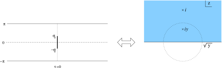
Figure 7: Mandelstam map for the strip with a slit into the upper half plane. The point at $\tau=\pm\infty$ map to $z=iy$ and $z=i$ whereas the slit maps to the real axis. The dotted line at $\tau=0$ and $\sigma_{0}\leq|\sigma|\leq\pi$ maps to the half circle of radius $\sqrt{y}$.

There is a sign ambiguity that has to be fixed. One can easily see that for $u\rightarrow 0$ we should take $z_{+}$ and for $u\rightarrow\infty$ we should use $z_{-}$. Off course by appropriately defining the cut in the square root we obtain a function analytic in the region parameterized by $\rho$. In the regions $u\rightarrow 0$ and $u\rightarrow\infty$ we can get a series expansion as:

$$z_{1}(u) = z_{+}(u)=\sum_{m=0}^{\infty}a_{m}u^{m},$$ (1.159)

$$z_{2}(u) = z_{-}(u)=\sum_{m=0}^{\infty}\frac{b_{m}}{u^{m}}.$$ (1.160)

We already know that $a_{0}=i$ and $b_{0}=iy$. The other coefficients are given by

$$a_{m} = \frac{2i}{m(1+\sin\frac{\sigma_{0}}{2})}\sum_{l=1}^{m}\frac{m!}{(m+l)!}l(-)^{l}\left[\frac{1+\sin\frac{\sigma_{0}}{2}}{\cos\frac{\sigma_{0}}{2}}\right]^{l}\mathrm{P}^{l}_{m}(\cos\sigma_{0})$$ (1.161)

$$= 2i\frac{\sin\frac{\sigma_{0}}{2}}{1+\sin\frac{\sigma_{0}}{2}}+\frac{i}{1+\sin\frac{\sigma_{0}}{2}}\sum_{l=1}^{m}\frac{1}{l}\left[\mathrm{P}_{l-2}(\cos\sigma_{0})-\cos\sigma_{0}\mathrm{P}_{l-1}(\cos\sigma_{0})\right],$$ (1.162)

$$b_{m} = \frac{2i}{m(1+\sin\frac{\sigma_{0}}{2})}\sum_{l=1}^{m}\frac{m!}{(m+l)!}l\left[\frac{\cos\frac{\sigma_{0}}{2}}{1+\sin\frac{\sigma_{0}}{2}}\right]^{l}\mathrm{P}^{l}_{m}(\cos\sigma_{0})$$ (1.163)

$$= -2i\frac{\sin\frac{\sigma_{0}}{2}}{1+\sin\frac{\sigma_{0}}{2}}+\frac{i}{1+\sin\frac{\sigma_{0}}{2}}\sum_{l=1}^{m}\frac{1}{l}\left[\mathrm{P}_{l-2}(\cos\sigma_{0})-\cos\sigma_{0}\mathrm{P}_{l-1}(\cos\sigma_{0})\right],$$ (1.164)

where we gave two alternative expressions. The first uses associated Legendre functions $\mathrm{P}^{l}_{m}(\cos\sigma_{0})$ and the other Legendre polynomials.

Once we have mapped the problem to the upper half plane, computing the Green function is trivial. We obtain

$$G(z,z^{\prime})=\ln|z-z^{\prime}|+\varepsilon_{i}\ln|z-\bar{z}^{\prime}|,$$ (1.165)

where $\varepsilon_{i}=1$ for Neumann boundary conditions and $\varepsilon_{i}=-1$ for Dirichlet. We can define now four functions

$$\mathrm{N}^{rs}(u,u^{\prime})=G(z_{r}(u),z_{s}(u^{\prime}))-\delta^{rs}\ln|u-u^{\prime}|,$$ (1.166)

with $r,s=1,2$ and we note that $\overline{z_{r}(u)}=-z_{r}(\bar{u})$. We also extracted the logarithmic singularity as is conventional. Each function can be expanded as a power series in $u$ and $u^{\prime}$ using (1.160). After that we replace $u=e^{i\sigma}$, $u^{\prime}=e^{i\sigma^{\prime}}$. Thus, we obtain

$$\mathrm{N}^{rs}(u,u^{\prime})=\sum_{m,n=\infty}^{\infty}\mathrm{N}^{rs}_{mn}(\varepsilon_{i},\sigma_{0})e^{in\sigma}e^{im\sigma^{\prime}}.$$ (1.167)

The coefficients $\mathrm{N}^{rs}_{mn}(\varepsilon_{i},\sigma_{0})$ are precisely the Neumann coefficients we want to find. If we expand $G$ we obtain coefficients

$$G^{rs}_{mn}=\mathrm{N}^{rs}_{mn}-\frac{1}{2|n|}\delta_{n+m}\delta^{rs}.$$ (1.168)

The difference is just the expansion of $\ln|u-u^{\prime}|$.

A straight-forward Taylor expansion can be used to compute a few of the coefficients. A more practical method of computation uses a trick. It is based on the fact that, by using the chain rule, we can obtain that

$$(\partial_{\sigma}+\partial_{\sigma^{\prime}})G = (1+\varepsilon_{i})\frac{z+\bar{z}+z^{\prime}+\bar{z}^{\prime}}{4(1-y)}$$ (1.171)

$$+\frac{\sqrt{y}(1+y)^{2}}{8(1-y)}\left[\left(\frac{1}{z+\sqrt{y}}+\frac{\varepsilon_{i}}{\bar{z}+\sqrt{y}}\right)\left(\frac{1}{z^{\prime}+\sqrt{y}}+\frac{\varepsilon_{i}}{\bar{z}^{\prime}+\sqrt{y}}\right)\right.$$

$$\left.-\left(\frac{1}{z-\sqrt{y}}+\frac{\varepsilon_{i}}{\bar{z}-\sqrt{y}}\right)\left(\frac{1}{z^{\prime}-\sqrt{y}}+\frac{\varepsilon_{i}}{\bar{z}^{\prime}-\sqrt{y}}\right)\right],$$

the right hand side is a sum of terms which are factorized, namely are a product of a function of $z$ times a function of $z^{\prime}$. We can then expand each of them and multiply the coefficients. The result is

$$\mathrm{N}^{rs}_{mn}(\varepsilon_{i},\sigma_{0})=-\frac{i}{8}\frac{(1+\varepsilon_{i})}{m+n}\left(a^{r}_{m}\delta_{n0}+a^{s}_{n}\delta_{m0}\right)+\frac{1}{(m+n)\sin\sigma_{0}}\mathrm{Im}\left(f^{r}_{m}f^{s}_{n}\right),$$ (1.172)

where

$$a^{1,2}_{m}=2i\pm\frac{i}{\sin\frac{\sigma_{0}}{2}}\sum_{l=1}^{m}\frac{1}{l}\left(\mathrm{P}_{l-2}(\cos\sigma_{0})-\cos\sigma_{0}\mathrm{P}_{l-1}(\cos\sigma_{0})\right),\ \ \ m>0,$$ (1.173)

and $a^{r}_{m}=-a^{r}_{-m}$. The coefficients $f^{r}_{m}$ are given by

$$f^{1}_{m>0}=-\bar{f}_{m},\ \ \ f^{1}_{m<0}=-\varepsilon_{i}f_{-m},\ \ \ f^{2}_{m\neq 0}=-\varepsilon_{i}f^{1}_{m},$$ (1.174)

with

$$f_{m>0}=-\frac{i}{m}e^{i\frac{\sigma_{0}}{2}}\sum_{l=1}^{m}\frac{(-i)^{l}m!}{(m+l)!}l\mathrm{P}^{l}_{m}(\cos\sigma_{0}).$$ (1.175)

Also,

$$f^{1}_{0} = \frac{1}{2}\left[(1+\varepsilon_{i})(1-\sin\frac{\sigma_{0}}{2})-i(1-\varepsilon_{i})\cos\frac{\sigma_{0}}{2}\right],$$ (1.176)

$$f^{2}_{0} = \frac{1}{2}\left[(1+\varepsilon_{i})(1+\sin\frac{\sigma_{0}}{2})-i(1-\varepsilon_{i})\cos\frac{\sigma_{0}}{2}\right].$$ (1.177)

The result is valid when $m+n\neq 0$. If not we obtain

$$N^{11}_{m,-m} = -\frac{\varepsilon_{i}}{2m^{2}}\left\{\sum_{l=1}^{m-1}l\frac{m!(m-l-1)!}{(m+l)!(m-1)!}\mathrm{P}^{l}_{m}(\cos\sigma_{0})\mathrm{P}^{l}_{m-1}(\cos\sigma_{0})\right.$$ (1.181)

$$\left.+\frac{(-)^{m}mz_{4}^{m}}{(1-z_{4})^{2m-1}}\left(\begin{array}[]{c}2m-1\\ m-1\end{array}\right)F(1,1-m;m+1;z_{4})\right\},$$

and

$$N^{12}_{m,-m}+\varepsilon_{i}N^{11}_{m,-m}=-\frac{1}{2|m|},$$ (1.182)

where $z_{4}=-\frac{\sin^{2}\frac{\sigma_{0}}{2}}{\cos^{2}\frac{\sigma_{0}}{2}}$ and $F$ denotes a hypergeometric function which in this case reduces to a polynomial. We also have

$$N^{rs}_{i,00}=(1+\epsilon_{i})\delta^{rs}\ln\left(\cos\frac{\sigma_{0}}{2}\right)+\frac{1-\epsilon_{i}}{2}\ln\left(\sin\frac{\sigma_{0}}{2}\right).$$ (1.183)

To obtain the results we used the fact that $f_{m}$ and $a_{m}$ can be represented as contour integrals through

$$f_{m}(y) = \frac{i\,\sqrt{y}}{2\pi m}\oint_{i}dz\frac{1}{(z-\sqrt{y})^{2}}\left(\frac{(z+i)(z-iy)}{(z-i)(z+iy)}\right)^{m},$$ (1.184)

$$a_{m}(y) = -\frac{i}{2\pi m}\oint_{i}dz\left(\frac{(z+i)(z-iy)}{(z-i)(z+iy)}\right)^{m}.$$ (1.185)

where the parameter $y$ was defined in eq.(1.157). Here $a_{m}$ is the one defined in (1.161) and is related to $a^{r}_{m}$ due to eq.(1.171) by

$$a^{1}_{m}=\frac{2}{1-y}\,a_{m}=\frac{1+\sin\frac{\sigma_{0}}{2}}{\sin\frac{\sigma_{0}}{2}}\,a_{m},\ \ (m\geq 1)$$ (1.186)

Using the method of residues we obtained the result in terms of sums that can be computed using

$$\sum_{p=0}^{m-l}\left(\begin{array}[]{c}m\\ p\end{array}\right)\left(\begin{array}[]{c}m\\ p+l\end{array}\right)\left(-\frac{1-\cos\sigma_{0}}{1+\cos\sigma_{0}}\right)^{p}=\frac{2^{m}m!}{(m+l)!}\frac{(-1)^{l}}{(1+\cos\sigma_{0})^{m}}\left(\frac{\sin\sigma_{0}}{1+\cos\sigma_{0}}\right)^{l}\mathrm{P}^{l}_{m}(\cos\sigma_{0})$$ (1.187)

To avoid confusion we recall the definition of associated Legendre functions:

$$\mathrm{P}^{l}_{m}(x)=(-1)^{l}(1-x^{2})^{\frac{l}{2}}\frac{d^{l}}{dx^{l}}\mathrm{P}_{m}(x)$$ (1.188)

where $P_{m}(x)$ are the standard Legendre polynomials.

A.1 Properties of the Neumann coefficients

From the calculation we did one can find the following identities

$$N^{12}_{mn}+\varepsilon_{i}N^{22}_{mn} = -\frac{1}{2|m|}\delta_{n,-m}+\frac{(1+\varepsilon_{i})}{2|m|}\delta_{n0},\ \ \ m\neq 0,$$ (1.189)

$$N^{12}_{mn}+\varepsilon_{i}N^{11}_{mn} = -\frac{1}{2|n|}\delta_{m,-n}+\frac{(1+\varepsilon_{i})}{2|n|}\delta_{m0},\ \ \ n\neq 0.$$ (1.190)

Other identities follow from the value of $G$ at $\tau=0$. For example, from the Dirichlet boundary condition, we know that, if $\varepsilon_{i}=-1$, then $G(\sigma,\sigma^{\prime})=0$ for $-\sigma_{0}<\sigma<\sigma_{0}$. In terms of Fourier components this can be written as

$$\sum_{n}e^{in\sigma}G^{rs}_{nm}=0,\ \ \ -\sigma_{0}<\sigma<\sigma_{0},\ \ \varepsilon_{i}=-1,$$ (1.191)

In the same way we can derive other identities. They follow from the value of $z$ when $\tau=0$. A simple calculation reveals that $z_{+}(e^{i\phi})$ is real for $-\sigma_{0}<\phi<\sigma_{0}$ and is equal to $z_{+}(e^{i\phi})=\sqrt{y}e^{i\Phi}$ for $\sigma_{0}<\phi<2\pi-\sigma_{0}$ with $\cos\Phi=-\tan\frac{\sigma_{0}}{2}\mathrm{cotan}\frac{\phi}{2}$. This means that the circle $\tau=0$ maps to the real axis and a circle of radius $\sqrt{y}$. The two sides of the slit map to different regions of the real axis corresponding to $|\mathrm{Re}(z)|$ greater or smaller than $\sqrt{y}$. If $z$ is real and $\varepsilon_{i}=-1$ then $G(z,z^{\prime})=0$ which is what we used to derive eq.(1.191). If $\varepsilon_{i}=1$ then it seems that $\mathrm{Im}(\partial_{z}G)=0$ if $z$ is real, but there is a possible singularity if $z^{\prime}$ is also real. Taking $z^{\prime}=x^{\prime}$ real and taking the limit $z\rightarrow x$ we get

$$\mathrm{Im}(\partial_{z}G)=-\pi\delta(x-x^{\prime}).$$ (1.192)

Going to variables $\phi$ ,$\phi^{\prime}$ and taking the Fourier transform we obtain

$$\sum_{n}|n|e^{in\phi}\mathrm{N}^{rs}_{mn}=-\frac{1}{2}e^{-im\phi}\delta_{r\neq s},$$ (1.193)

where $\delta_{r\neq s}=1-\delta_{rs}$. To get this result we used (1.168) and the fact that $\delta(x-x^{\prime})$ on eq.(1.192) contributes only if $x$ can be equal to $x^{\prime}$ which happens if $r=s$, namely both points are on the same side of the slit.

The next property is related to the values of the Green function for $\sigma_{0}<\phi<2\pi-\sigma_{0}$. A lengthy but not difficult calculation reveals that

$$\mathrm{Re}(\partial_{\rho}G)=-\frac{\pi}{2}\delta(\phi-\phi^{\prime}),\ \ \ \varepsilon_{i}=-1,\ \ u=e^{i\phi},\ \ u^{\prime}=e^{i\phi^{\prime}},\ \ \sigma_{0}<\phi<2\pi-\sigma_{0}.$$ (1.194)

Again, doing a Fourier transform and using (1.168) we obtain

$$\sum_{n}|n|e^{in\phi}\mathrm{N}^{rs}_{mn}=-\frac{1}{2}e^{-im\phi}\delta^{r\neq s},\ \ \ \ \varepsilon_{i}=-1.$$ (1.195)

The equivalent identity for $\varepsilon_{i}=1$ is a little more difficult to derive. We start from the expression for $G$ and replace $z_{+}=\sqrt{y}e^{i\Phi}$. We do the same for $z^{\prime}$ but we need to consider two cases, when $-\sigma_{0}<\phi^{\prime}<\sigma_{0}$ and when $\sigma_{0}<\phi^{\prime}<2\pi-\sigma_{0}$. Then we can compute $G$ and obtain that

$$G^{11} = \ln\frac{\sin\frac{\sigma_{0}}{2}}{1+\sin\frac{\sigma_{0}}{2}}+\ln|e^{i\phi}-e^{i\phi^{\prime}}|-\ln|\frac{1-e^{-i\phi^{\prime}}}{2}|-\ln|\frac{1-e^{-i\phi}}{2}|+\frac{1}{2}(\ln z^{\prime}+\ln\bar{z}^{\prime}),$$

for $$\varepsilon_{i}=1,\ \ \sigma_{0}<\phi<2\pi-\sigma_{0}.$$ (1.196)

We only computed $G^{11}$ since the others follow from the identities (1.190). From the relation between $\rho$ and $z$ one finds that

$$\frac{(u-1)^{2}}{u}=-\frac{4z^{2}(1-y)^{2}}{(1+z^{2})(z^{2}+y^{2})}.$$ (1.197)

Taking logarithms on both sides and taking the real part we find that

$$2\ln z+2\ln\bar{z}=G(z,i)+G(z,iy)-4\ln 2-4\ln(1-y)+4\ln|1-u|-2\ln|u|,$$ (1.198)

where the Green function is taken with $\varepsilon_{i}=1$. Doing a Fourier transform we find that

$$\ln z+\ln\bar{z}=\sum_{n}\alpha_{n}e^{in\phi},\ \ \ \alpha_{n\neq 0}=\mathrm{N}^{11}_{n0}+\mathrm{N}^{12}_{n0}-\frac{1}{|n|},\ \ \varepsilon_{i}=+1.$$ (1.199)

Using this we can expand (1.196) to obtain

$$\sum_{n}e^{in\phi}\mathrm{N}^{11}_{nm}=\frac{1}{2}(\mathrm{N}^{11}_{n0}+\mathrm{N}^{12}_{n0}),\ \ \ \sigma_{0}<\phi<2\pi-\sigma_{0},$$ (1.200)

i.e. the function of $\phi$ on the left is actually a constant in that interval.

We can summarize the properties of $\mathrm{N}^{rs}_{mn}$ as

• $\varepsilon_{i}=-1$ (Dirichlet)

  $$\begin{array}[]{lcl}\sum_{n}e^{in\phi}\mathrm{N}^{rs}_{mn}=\frac{1}{2|m|}e^{-im\phi}\delta^{rs},&&-\sigma_{0}<\phi<\sigma_{0}\\ &&\\ \sum_{n}|n|e^{in\phi}\mathrm{N}^{rs}_{mn}=-\frac{1}{2|m|}e^{-im\phi}\delta^{r\neq s},&&\sigma_{0}<\phi<2\pi-\sigma_{0},\end{array}$$ (1.201)

• $\varepsilon_{i}=+1$ (Neumann)

  $$\begin{array}[]{lcl}\sum_{n=-\infty}^{\infty}|n|e^{in\phi}\mathrm{N}^{rs}_{mn}=-\frac{1}{2}e^{-im\phi}\delta^{rs},&&-\sigma_{0}<\phi<\sigma_{0}\\ &&\\ \sum_{n}e^{in\phi}\mathrm{N}^{rs}_{mn}=\frac{1}{2|m|}(2-e^{-im\phi})\delta^{r\neq s}+(\mathrm{N}^{11}_{n0}+\mathrm{N}^{12}_{n0})(\delta^{rs}-\frac{1}{2}),&&\sigma_{0}<\phi<2\pi-\sigma_{0},\end{array}$$ (1.202)

Other useful relations are:

$$N^{11}_{nm}(\varepsilon_{i}=-1) = \mathrm{sign}(n)\,\mathrm{sign}(m)\,N^{11}_{nm}(\varepsilon_{i}=+1),\ \ \ \ (m,n\neq 0)$$ (1.203)

$$N^{12}_{nm}(\varepsilon_{i}=-1) = -\mathrm{sign}(n)\,\mathrm{sign}(m)\,N^{12}_{nm}(\varepsilon_{i}=+1),\ \ \ \ (m,n\neq 0)$$ (1.204)

which can be used to derive

$$\sum_{n\neq 0}\mathrm{sign}(n)N^{11}_{nm}(\varepsilon_{i}=-1)e^{in\sigma} = \frac{1}{2}\mathrm{sign}(m)\left\{N^{12}_{m0}(\varepsilon_{i}=+1)-N^{11}_{m0}(\varepsilon_{i}=+1)\right\}$$ (1.205)

$$\sum_{n\neq 0}\mathrm{sign}(n)N^{12}_{nm}(\varepsilon_{i}=-1)e^{in\sigma} = \frac{1}{2m}e^{-im\sigma}+\frac{1}{2}\mathrm{sign}(m)\left\{N^{12}_{m0}(\varepsilon_{i}=+1)-N^{11}_{m0}(\varepsilon_{i}=+1)\right\}$$

A.2 Limit of large subindex

It is useful to understand also various limits of the Neumann coefficients. One is their behavior for large values of one subindex. In view of the expression (1.172) we only need to know the behavior of $a_{m}$ and $f_{m}$ for large $m$. These coefficients can be computed by an integral in the complex plane which can be evaluated by a saddle point approximation. In terms of the parameter $y$ defined in eq.(1.157) we have

$$f_{m}(y) = \frac{i\,\sqrt{y}}{2\pi m}\oint_{i}dz\frac{1}{(z-\sqrt{y})^{2}}\left(\frac{(z+i)(z-iy)}{(z-i)(z+iy)}\right)^{m},$$ (1.206)

$$a_{m}(y) = -\frac{i}{2\pi m}\oint_{i}dz\left(\frac{(z+i)(z-iy)}{(z-i)(z+iy)}\right)^{m}.$$ (1.207)

To understand the saddle point calculation it is useful to plot numerically the absolute value of the integrand as a function of $z$. This is a useful aid to clarify the position of the saddle points. In any case, a standard calculation gives

$$f_{m} \simeq_{m\rightarrow\infty} \frac{\sqrt{\sin\sigma_{0}}}{\sqrt{2\pi m}}e^{-i\frac{\pi}{4}}e^{im\sigma_{0}},$$ (1.208)

$$a^{1}_{m} \simeq_{m\rightarrow\infty} 4i-\frac{2i}{\sqrt{2\pi}}\frac{1}{m^{\frac{3}{2}}}\frac{\cos\frac{\sigma_{0}}{2}}{\sin\frac{\sigma_{0}}{2}}\frac{1}{\sqrt{\sin\sigma_{0}}}\cos\left(m\sigma_{0}-\frac{\pi}{4}\right),$$ (1.209)

$$a^{2}_{m} \simeq_{m\rightarrow\infty} \frac{2i}{\sqrt{2\pi}}\frac{1}{m^{\frac{3}{2}}}\frac{\cos\frac{\sigma_{0}}{2}}{\sin\frac{\sigma_{0}}{2}}\frac{1}{\sqrt{\sin\sigma_{0}}}\cos\left(m\sigma_{0}-\frac{\pi}{4}\right).$$ (1.210)

Except for the constant part, the coefficients $a_{m}$ are subleading and can be ignored. For $m\rightarrow\infty$ the contribution comes from $f_{m}$.

A.3 Limit $\sigma_{0}\rightarrow 0$

Other limit of interest are $\sigma_{0}\rightarrow 0$. Using standard properties of the Legendre polynomials one can derive that the functions $f_{m>0}(\sigma_{0})$, $a^{r}_{m}(\sigma_{0})$ and $f^{r}_{0}(\sigma_{0})$ which enter in the formula for the Neumann coefficients behave as:

$$f_{m>0}(\sigma_{0}) \simeq \frac{\sigma_{0}}{2}\left(1+\frac{i\sigma_{0}}{2}m-\frac{\sigma_{0}^{2}}{4}\left(m^{2}+\frac{1}{6}\right)+\ldots\right),$$ (1.211)

$$f^{1}_{0}(\sigma_{0}) \simeq \frac{1}{2}\left[(1+\varepsilon_{i})-i(1-\varepsilon_{i})\right]-\frac{1+\varepsilon_{i}}{4}\sigma_{0}+\frac{i}{16}(1-\varepsilon_{i})\sigma_{0}^{2}+\ldots,$$ (1.212)

$$f^{2}_{0}(\sigma_{0}) \simeq \frac{1}{2}\left[(1+\varepsilon_{i})-i(1-\varepsilon_{i})\right]+\frac{1+\varepsilon_{i}}{4}\sigma_{0}+\frac{i}{16}(1-\varepsilon_{i})\sigma_{0}^{2}+\ldots,$$ (1.213)

$$a^{1,2}_{m}(\sigma_{0}) \simeq 2i\left(1\pm\frac{\sigma_{0}}{2}m+\ldots\right).$$ (1.214)

From here we can obtain the behavior of $\mathrm{N}^{rs}_{mn}$. Assuming that $m,n>0$ we obtain that

$$\mathrm{N}^{rr}_{mn}\simeq-\frac{1}{8}\sigma_{0}^{2},\ \ \mathrm{N}^{rr}_{m,-n}\simeq-\frac{\varepsilon_{i}}{8}\sigma_{0}^{2},\ \ \mathrm{N}^{rr}_{-m,-n}\simeq-\frac{1}{8}\sigma_{0}^{2},\ \ (\sigma_{0}\rightarrow 0)$$ (1.215)

which together with the properties (1.190) of $\mathrm{N}^{rs}_{mn}$ determine completely the small $\sigma_{0}$ behavior when $m,n\neq 0$. Note that, in particular, (1.190) implies that

$$N^{12}_{m,-m}\simeq-\frac{1}{2|m|}+\frac{\sigma_{0}^{2}}{8}+\ldots,$$ (1.216)

has an order zero contribution. In the case that one subindex is zero we get

$$N^{11}_{m0} \simeq \frac{1}{2|m|}+\frac{1+\varepsilon_{i}}{4}\sigma_{0}-\frac{\sigma_{0}^{2}}{16}\left[(1+\varepsilon_{i})+|m|(1-\varepsilon_{i})\right]+\ldots,$$ (1.217)

$$N^{12}_{m0} \simeq \frac{1}{2|m|}+\frac{1+\varepsilon_{i}}{4}\sigma_{0}-\frac{\sigma_{0}^{2}}{16}\left[-(1+\varepsilon_{i})+|m|(1-\varepsilon_{i})\right]+\ldots,$$ (1.218)

$$N^{21}_{m0} \simeq \frac{1}{2|m|}-\frac{1+\varepsilon_{i}}{4}\sigma_{0}-\frac{\sigma_{0}^{2}}{16}\left[-(1+\varepsilon_{i})+|m|(1-\varepsilon_{i})\right]+\ldots,$$ (1.219)

$$N^{22}_{m0} \simeq \frac{1}{2|m|}-\frac{1+\varepsilon_{i}}{4}\sigma_{0}-\frac{\sigma_{0}^{2}}{16}\left[(1+\varepsilon_{i})+|m|(1-\varepsilon_{i})\right]+\ldots.$$ (1.220)

Where in all cases we have expanded to the order that is necessary for the main part of the paper.

References

• [1] G.’t Hooft, Nucl. Phys. B72 (1974) 461, G.’t Hooft, Nucl. Phys. B75 (1974) 461.
• [2] J. Polchinski, “Dirichlet-Branes and Ramond-Ramond Charges,” Phys. Rev. Lett.  75, 4724 (1995) [arXiv:hep-th/9510017].
• [3] J. Maldacena, “The large $N$ limit of superconformal field theories and supergravity,” Adv. Theor. Math. Phys.  2, 231 (1998) [Int. J. Theor. Phys.  38, 1113 (1998)], hep-th/9711200,
S. S. Gubser, I. R. Klebanov and A. M. Polyakov, “Gauge theory correlators from non-critical string theory,” Phys. Lett. B 428, 105 (1998) [arXiv:hep-th/9802109],
E. Witten, “Anti-de Sitter space and holography,” Adv. Theor. Math. Phys.  2, 253 (1998) [arXiv:hep-th/9802150],
O. Aharony, S. S. Gubser, J. M. Maldacena, H. Ooguri and Y. Oz, “Large N field theories, string theory and gravity,” Phys. Rept.  323, 183 (2000) [arXiv:hep-th/9905111].
• [4] R. R. Metsaev and A. A. Tseytlin, “Type IIB superstring action in AdS(5) x S(5) background,” Nucl. Phys. B 533, 109 (1998) [arXiv:hep-th/9805028].
• [5] L. Brink, O. Lindgren and B. E. W. Nilsson, “N=4 Yang-Mills Theory On The Light Cone,” Nucl. Phys. B 212, 401 (1983),
S. Mandelstam, “Light Cone Superspace And The Ultraviolet Finiteness Of The N=4 Model,” Nucl. Phys. B 213, 149 (1983) ,
L. Brink, O. Lindgren and B. E. W. Nilsson, “The Ultraviolet Finiteness Of The N=4 Yang-Mills Theory,” Phys. Lett. B 123, 323 (1983).
• [6] K. Bardakci and C. B. Thorn, “A worldsheet description of large N(c) quantum field theory,” Nucl. Phys. B 626, 287 (2002) [arXiv:hep-th/0110301]
C. B. Thorn, “A worldsheet description of planar Yang-Mills theory,” Nucl. Phys. B 637, 272 (2002) [Erratum-ibid. B 648, 457 (2003)] [arXiv:hep-th/0203167].
• [7] A. Clark, A. Karch, P. Kovtun and D. Yamada, “Construction of bosonic string theory on infinitely curved anti-de Sitter space,” Phys. Rev. D 68, 066011 (2003) [arXiv:hep-th/0304107].
• [8] R. Gopakumar, “From free fields to AdS,” Phys. Rev. D 70, 025009 (2004) [arXiv:hep-th/0308184].
• [9] O. Aharony, Z. Komargodski and S. S. Razamat, arXiv:hep-th/0602226.
• [10] S. J. Brodsky, H. C. Pauli and S. S. Pinsky, “Quantum chromodynamics and other field theories on the light cone,” Phys. Rept.  301, 299 (1998) [arXiv:hep-ph/9705477].
• [11] C. B. Thorn, “Notes on one-loop calculations in light-cone gauge,” arXiv:hep-th/0507213.
• [12] A. V. Belitsky, S. E. Derkachov, G. P. Korchemsky and A. N. Manashov, “Dilatation operator in (super-)Yang-Mills theories on the light-cone,” Nucl. Phys. B 708, 115 (2005) [arXiv:hep-th/0409120].
• [13] M. B. Green, J. H. Schwarz and E. Witten, “Superstring Theory. Vol. 2: Loop Amplitudes, Anomalies And Phenomenology,” Cambridge University Press 1995. In particular see Chapter 11.
• [14] M. B. Green, J. H. Schwarz and L. Brink, “Superfield Theory Of Type II Superstrings,” Nucl. Phys. B 219, 437 (1983).
• [15] M. B. Green and J. H. Schwarz, “Superstring Field Theory,” Nucl. Phys. B 243, 475 (1984).
• [16] M. Spradlin and A. Volovich, “Superstring interactions in a pp-wave background,” Phys. Rev. D 66, 086004 (2002) [arXiv:hep-th/0204146],
A. Pankiewicz and B. . J. Stefanski, “pp-wave light-cone superstring field theory,” Nucl. Phys. B 657, 79 (2003) [arXiv:hep-th/0210246].
• [17] A. M. Polyakov, “Gauge fields and space-time,” Int. J. Mod. Phys. A 17S1, 119 (2002) [arXiv:hep-th/0110196].
• [18] J. Greensite and F. R. Klinkhamer, “Superstring Amplitudes And Contact Interactions,” Nucl. Phys. B 304, 108 (1988).
• [19] R. R. Metsaev, C. B. Thorn and A. A. Tseytlin, “Light-cone superstring in AdS space-time,” Nucl. Phys. B 596, 151 (2001) [arXiv:hep-th/0009171].
• [20] J. Polchinski and L. Susskind, “String theory and the size of hadrons,” arXiv:hep-th/0112204.
• [21] M. B. Green and P. Wai, “The Insertion of boundaries in world sheets,” Nucl. Phys. B 431, 131 (1994).
• [22] P. Di Vecchia and A. Liccardo, “D branes in string theory. I,” NATO Adv. Study Inst. Ser. C. Math. Phys. Sci.  556, 1 (2000) [arXiv:hep-th/9912161].
• [23] I. R. Klebanov and L. Thorlacius, “The Size of p-Branes,” Phys. Lett. B 371, 51 (1996) [arXiv:hep-th/9510200],
M. R. Garousi and R. C. Myers, “Superstring Scattering from D-Branes,” Nucl. Phys. B 475, 193 (1996) [arXiv:hep-th/9603194],
A. Hashimoto and I. R. Klebanov, “Scattering of strings from D-branes,” Nucl. Phys. Proc. Suppl.  55B, 118 (1997) [arXiv:hep-th/9611214].
• [24] W. Fischler, I. R. Klebanov and L. Susskind, “String Loop Divergences And Effective Lagrangians,” Nucl. Phys. B 306, 271 (1988).