ITEP/TH - 08/06

INR/TH - 06-2006

Quantum Field Theory as Effective BV Theory from Chern-Simons

Dmitry Krotov^a and Andrei Losev^b

^aInstitute for Nuclear Research of the Russian Academy of Sciences,
60th October Anniversary prospect 7a, Moscow, 117312, Russia
^a,bInstitute of Theoretical and Experimental Physics,
B.Cheremushkinskaya 25, Moscow, 117259, Russia
^aMoscow State University, Department of Physics,
Vorobjevy Gory, Moscow, 119899, Russia

ABSTRACT

The general procedure for obtaining explicit expressions for all cohomologies of N.Berkovits’s operator is suggested. It is demonstrated that calculation of BV integral for the classical Chern-Simons-like theory (Witten’s OSFT-like theory) reproduces BV version of two dimensional gauge model at the level of effective action. This model contains gauge field, scalars, fermions and some other fields. We prove that this model is an example of "singular" point from the perspective of the suggested method for cohomology evaluation. For arbitrary "regular" point the same technique results in AKSZ(Alexandrov, Kontsevich, Schwarz, Zaboronsky) version of Chern-Simons theory (BF theory) in accord with [2, 3].

1 Introduction

The search for fundamental degrees of freedom is a challenging problem in physics. Different attempts in this direction demonstrated that Chern-Simons-like theories (Witten’s OSFT-like theories) play important role for questions of this type [1]. In the present paper we discuss a small subject in the story which to the best of our knowledge did not attract enough attention in the literature. We suggest the construction which allows to obtain a classical action for a large class of quantum field theories as effective Batalin-Vilkovisky(BV) action from the certain fundamental action (1). This realizes a beautiful idea that different "physically interesting" theories can arise in a universal way as effective actions from the certain fundamental theory. The technique is very much in the spirit of recently suggested formalism for covariant quantization of the superparticle [2] and the superstring [7] by N.Berkovits. Close ideas were discussed in [3]-[5] and in [6].

The basis of construction is the space (algebra) $O[\theta_{\alpha}\ \!,\ \!\lambda_{\alpha}\ |\ f^{\mu}(\lambda)]$ which is generated by the set of odd variables $\theta_{\alpha}$, even variables $\lambda_{\alpha}$ modulo the system of constraints $f^{\mu}(\lambda)$, quadratic in $\lambda_{\alpha}$ ($\alpha=1...K$, $\mu=1...N$). This means that if some function of $\lambda$ and $\theta$ is multiplied by $f^{\mu}(\lambda)$, such product is equivalent to zero in the space $O[\theta_{\alpha}\ \!,\ \!\lambda_{\alpha}\ |\ f^{\mu}(\lambda)]$. In other words, one should consider the supercommutative ring $C[\lambda,\ \theta]$ of polynomials in $\lambda_{\alpha}$ and $\theta_{\alpha}$. This ring contains the ideal $I_{f}$ which is generated by the set of quadratic constraints $f^{\mu}(\lambda)$, i.e. arbitrary element in $I_{f}$ can be written as $c_{\mu}(\lambda,\theta)f^{\mu}(\lambda)$ where coefficients $c_{\mu}(\lambda,\theta)\in C[\lambda,\ \theta]$ belong to the ring $C[\lambda,\theta]$. The space $O[\theta_{\alpha}\ \!,\ \!\lambda_{\alpha}\ |\ f^{\mu}(\lambda)]$ is given by the coset $O[\theta_{\alpha}\ \!,\ \!\lambda_{\alpha}\ |\ f^{\mu}(\lambda)]=C[\lambda,\ \theta]\diagup I_{f}$.

In the recent discussions [2, 7, 17] notation $\lambda_{\alpha}$ was used for pure spinor variables which satisfy pure spinor constraints $f^{\mu}(\lambda)\ =\ \lambda_{\alpha}\gamma^{\mu}_{\alpha\beta}\lambda_{\beta}$. One message of the present paper is to relax this condition and to consider arbitrary system of constraints $f^{\mu}(\lambda)$, quadratic in $\lambda_{\alpha}$, which are not necessarily connected to $\gamma$ - matrices. It will be demonstrated that this setup leads to non-trivial effective gauge model at least in two dimensions. Thus, since $\lambda_{\alpha}$ are no longer pure spinors, we call them simply even variables and functions $f^{\mu}(\lambda)$ which generalize pure spinor constraints - simply constraints (generating the ideal $I_{f}$).

The construction starts from the fundamental action written as

$$S^{Fund}\ =\ \int\ STr\Big{(}<\mathcal{P},\ Q_{B}\mathcal{A}>\ +\ g<\mathcal{P},\ \mathcal{A}^{2}>\Big{)}$$ (1)

where the field $\mathcal{A}$ belongs to space $O[\theta_{\alpha}\ \!,\ \!\lambda_{\alpha}\ |\ f^{\mu}(\lambda)]\otimes Func(x)\otimes T(\mathfrak{g})$. $Func(x)$ is a space of functions of space-time coordinates and $T(\mathfrak{g})$ is a representation of semi-simple gauge algebra $\mathfrak{g}$. The field $\mathcal{P}$ belongs to the dual space $O[\theta_{\alpha}\ \!,\ \!\lambda_{\alpha}\ |\ f^{\mu}(\lambda)]^{\ast}\otimes Func(x)\otimes T(\mathfrak{g})$. Thus, each field belongs to space which is the tensor product of three spaces. To construct a scalar action from these fields introduce three pairings: integration - the pairing in the space $Func(x)$, $STr$ - the supertrace - the pairing in $T(\mathfrak{g})$ and $<\ ,\ >$ - the canonical paring between the elements of the space $O[\theta_{\alpha}\ \!,\ \!\lambda_{\alpha}\ |\ f^{\mu}(\lambda)]$ and the elements of $O[\theta_{\alpha}\ \!,\ \!\lambda_{\alpha}\ |\ f^{\mu}(\lambda)]^{\ast}$. The definition of the supertrace is given in the footnote 5. Parameter $g$ in the action (1) is a coupling constant.

The central object of our consideration is the operator [2, 7, 8]:

$$Q_{B}\ =\ Q\ +\ \Phi\ =\ \lambda_{\alpha}\frac{\partial}{\partial\theta_{\alpha}}\ +\ \theta_{\alpha}\frac{\partial f^{\mu}}{\partial\lambda_{\alpha}}\partial_{\mu}$$ (2)

Here $\partial_{\mu}=\frac{\partial}{\partial x^{\mu}}$ is a derivative with respect to the space-time coordinates. Operator $Q_{B}$ is nilpotent ($Q_{B}^{2}\ =\ 0$) in the space $O[\theta_{\alpha}\ \!,\ \!\lambda_{\alpha}\ |\ f^{\mu}(\lambda)]$ due to constraints $f^{\mu}(\lambda)$.

In [2, 7] it was suggested to extract dynamical fields of the theory from the cohomologies of $Q\ =\ \lambda_{\alpha}\frac{\partial}{\partial\theta_{\alpha}}$ operator ( the first term in (2) ). These cohomologies $\mathcal{H}(Q,\ O)$ or simply $\mathcal{H}(Q)$ should be calculated in the space $O[\theta_{\alpha}\ \!,\ \!\lambda_{\alpha}\ |\ f^{\mu}(\lambda)]$ which is given by the coset over the ideal $I_{f}$. Because of this factorization calculation of cohomologies is rather involved mathematical problem. It was attacked in [9]. In this paper effective method of localization was used to compute them. Such technique is very powerful in symmetric case (when the matrices $\gamma^{\mu}_{\alpha\beta}$ in the definition of quadrics $f^{\mu}(\lambda)\ =\ \lambda_{\alpha}\gamma^{\mu}_{\alpha\beta}\lambda_{\beta}$ are governed by some large group of symmetry).

In the present paper we suggest the general formulas which allow to find explicit expressions for all representatives of $\mathcal{H}(Q)$ for arbitrary system of quadrics $f^{\mu}(\lambda)$ (both in symmetric and non-symmetric cases). This calculation works in a universal way independently of the particular structure of functions $f^{\mu}(\lambda)$, their number $N$ ($\mu\ =\ 1...N$) and the number $K$ of $\lambda_{\alpha}$ and $\theta_{\alpha}$ ($\alpha\ =\ 1...K$). The description of this calculation is presented in the chapter 4 and in the appendix.

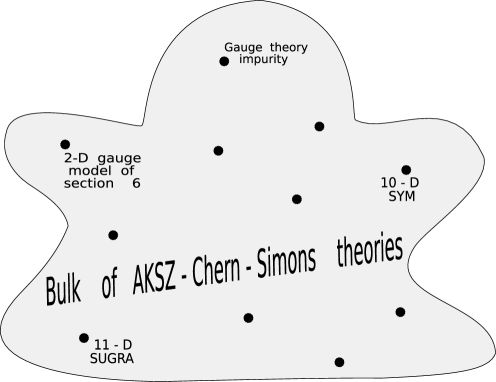
Figure 1: The space of effective theories. Black dots denote different gauge theories which are a kind of "singularities" in the bulk of AKSZ-Chern-Simons theories, which are denoted by gray background. This picture is in fact oversimplified and a little bit cheating. The more accurate one is given in the conclusion (see figure 14).

Another message of the present paper is to realize the construction of [2, 7] as calculation of effective action for the certain fundamental action (1). Close attempts were made in [3, 4]. The construction is given by the following steps. Firstly, using the powerful method of chapter 4 one should find explicit expressions for all representatives of $\mathcal{H}(Q)$. Then one should apply the background field technique to find effective action for (1) taking as external (background) field the representatives of $\mathcal{H}(Q)$. Effective action found in such a way reproduces BV version of some "physically interesting" theory.

According to this construction the whole information about degrees of freedom and the structure of effective theory is encoded in the representatives of $\mathcal{H}(Q)$, hence - in the system of quadrics $f^{\mu}(\lambda)$. From the perspective of the method of chapter 4 for cohomology evaluation there are two classes of quadrics $f^{\mu}(\lambda)$. They are: "regular" system and "singular" system. For arbitrary "regular" system of quadrics effective action is BV version of AKSZ-Chern-Simons theory. In section 5 we note that nearly all possible systems of quadrics $f^{\mu}(\lambda)$ are "regular". Still, there exists a small (but infinite) number of "singular" systems of quadrics. For such quadrics effective action is BV version of a non-trivial theory. One example of such "singular" point is the two-dimensional gauge model of section 6. Another one is 10D SYM theory of [2, 3] and probably even the supergravity theory of [14], see also [15]. This allows to think about "non-trivial" theories, like 10D SYM and super-gauge model of section 6, as a kind of "singularities" in the space of "trivial" theories of Chern-Simons type. This idea is illustrated in the figure 1. In this picture the bulk of trivial theories like Chern-Simons is denoted by gray background, while physically interesting gauge theories are denoted by black dots.

The universal feature of all these theories is that they are all supersymmetric. However in "regular" case this supersymmetry transformation acts by zero (see [18] for details).

Summarizing the introduction, we emphasize that the main new results of the present paper are:

1. Explicit expressions (4.1) for all representatives of $\mathcal{H}(Q,\ O)$ for arbitrary system of quadratic constraints $f^{\mu}(\lambda)$.

2. The two-dimensional gauge model of section 6 can be obtained as effective action from the theory (1). The classical action for this theory is given in (5). In the spectrum of this theory there are: gauge field (which is not dynamical), left and right fermions, adjoint scalars $\phi_{1}$ and $\phi_{2}$ and some other fields. The system of quadrics for this model is given by (1.1).

The quadrics (1.1) is the minimal system (minimal number of $\theta_{\alpha}$, $K\ =\ 4$ and minimal number of quadrics, $N\ =\ 5$) which reproduces kinetic term quadratic in derivatives in the effective action. It happens that this particular model is two-dimensional (d=2). It seems probable, that increasing the number of $\theta_{\alpha}$ ($K\ =\ 5,6,...$) and the number of quadrics ($N\ =\ 6,7,...$) one can obtain higher dimensional (d = 3,4,5,…) "physically interesting" theories in the "singular" points additionally to the known ones (10-D SYM and 11-D SUGRA). To our mind it is of interest to search for such "singular" points in the space of quadrics $f^{\mu}(\lambda)$. It is also of interest to study the string version of the model suggested in section 6.

1.1 Organization of the paper

Below we give the outline of each chapter of the paper. For those people who is interested in calculation of cohomologies $\mathcal{H}(Q,O)$ we recommend to read directly chapter 4. While our main result in this paper - the 2-D gauge model - is presented in chapter 6.

2. AKSZ Theory as BV Theory ……………………………………………………………………………………………………4

This chapter does not contain new results. It is a kind of introduction in some elementary facts about BV formalism. We give the definition of AKSZ-theory and explain why we are interested in this class of theories. Important statement is that the calculation of BV integral for the classical BV action reproduces effective action, which again satisfies BV Master Equation. It is explained that quantum calculations with the Faddeev-Popov action are equivalent to integration of BV action over the lagrangian sub-manifold. This technique is used in chapter 3.

3. Quantum Calculations ………………………………………………………………………………………………………………8

It is explained how one should conduct Feynman diagram calculations for the theory (1). This is non-trivial since the action (1) has a large gauge freedom, hence requires the choice of certain lagrangian sub-manifold. In our calculations this is equivalent to particular choice of gauge in the theory (1).

4. Calculation of Cohomologies ………………………………………………………………………………………………….10

This is the central chapter of the paper. It contains the new result - explicit expressions (4.1) for all cohomologies of $Q$-operator in the space $O[\theta_{\alpha}\ \!,\ \!\lambda_{\alpha}\ |\ f^{\mu}(\lambda)]$ (these cohomologies are usually called the zero-momentum cohomologies). Subsection 4.1 contains the description of the procedure, subsection 4.2 the brute force proof of this result. Another, more elegant proof is presented in the appendix. In the end of chapter 4 the definition of "regular" and "singular" system of quadrics is given.

5. AKSZ-Chern-Simons as Effective BV Theory …………………………………………………………………………15

In this chapter we present the calculation of effective BV action for the simplest possible example - 3-dimensional AKSZ version of Chern-Simons theory. The system of quadrics for this theory is given by:

$$f_{1}=\lambda_{1}^{2}$$

$$f_{2}=\lambda_{2}^{2}$$ (3)

$$f_{3}=\lambda_{3}^{2}$$

Though the answer for the cohomologies is almost obvious in this case, in section 5.1 we apply the general procedure of chapter 4 to find them. The aim of this calculation is to illustrate how the procedure works in this simplest case.

Then, in the subsection 5.2 we present the calculation of the 4-point amplitude in the theory (1), emphasizing all subtleties that are important for Feynman diagram calculations in such theories. At this step this calculation is just an illustration, clarifying the conventions we use. As we explain such amplitude is forbidden for the "regular" set (1.1). However, exactly this amplitude will be important in calculation of effective action for our main example - the 2-dimensional gauge model of section 6.

Subsection 5.3 contains the calculation of effective action for the system (1.1). The result is given in (40). It is demonstrated that (40) reproduces BV version of AKSZ-Chern-Simons theory from section 2.

In the subsection 5.4 it is proved that the same result (40) for the effective action is true for arbitrary "regular" system of quadrics, not necessarily restricted to the simple form (1.1). It is noted that nearly all possible systems of quadrics $f^{\mu}(\lambda)$ are "regular".

6. The Gauge Model ……………………………………………………………………………………………………………………20

This chapter contains our main result in the present paper. We suggest the example of "singular" system of quadrics:

$$f_{1}\ =\ \lambda_{1}\lambda_{2}$$

$$f_{2}\ =\ \lambda_{2}\lambda_{3}$$

$$f_{3}\ =\ \lambda_{3}\lambda_{4}$$ (4)

$$f_{4}\ \ \ =\ \ \lambda_{1}^{2}$$

$$f_{5}\ \ \ =\ \ \lambda_{4}^{2}$$

which under reduction over 3 dimensions reproduces BV action of 2-dimensional gauge model. The classical action, corresponding to this BV action is given by

$$\begin{split}I[A]\ =\ \int\ Tr\ \bigg{(}\ \Phi F_{+-}\ +\ D_{+}\phi_{1}D_{-}\phi_{1}\ +\ D_{-}\phi_{2}D_{+}\phi_{2}\ -\ \frac{g}{\sqrt{2}}\phi_{1}\{\psi_{+},\psi_{-}\}\ +\ i\frac{g}{\sqrt{2}}\phi_{2}\{\psi_{+},\psi_{-}\}\ +\ \beta_{+}D_{-}\gamma_{+}\ +\\ +\ \beta_{-}D_{+}\gamma_{-}\ +\ \overline{\psi}_{-}D_{+}\psi_{-}\ +\ \overline{\psi}_{+}D_{-}\psi_{+}\ +\ \overline{\chi}_{-}D_{+}\chi_{-}\ +\ \overline{\chi}_{+}D_{-}\chi_{+}\ +\ 2g\overline{\chi}_{-}[\gamma_{-},\psi_{+}]\ +\ 2g\overline{\chi}_{+}[\gamma_{+},\psi_{-}]\ \bigg{)}\end{split}$$ (5)

This model is another example of "physically interesting" theory which like 10-dimensional SYM arises from Berkovits construction for the "singular" systems of quadrics $f^{\mu}(\lambda)$. However, in comparison with 10-d SYM theory, this model is much simpler, hence is more calculable.

8. Appendix. Algebraic Meaning of the Berkovits Complex……………………………………………………..27

Another proof of the theorem from the section 4 is given. It is demonstrated that Berkovits complex naturally arises for the pure algebraic reasons.

2 AKSZ theory as BV theory

In this section we explain how AKSZ theory (definition is in the end of the section) arises from the general BV formalism for gauge theories [10, 11]. Consider a set of dynamical fields $\chi^{n}$ (arbitrary fields in our theory). For each field $\chi^{n}$, introduce an anti-field $\chi_{n}^{\ast}$ with the opposite statistics to $\chi^{n}$. Define the odd Laplace operator (BV laplacian) as $\Delta_{BV}\ =\ \int\frac{\delta_{L}}{\delta\chi^{n}(x)}\frac{\delta_{R}}{\delta\chi_{n}^{\ast}(x)}$. Here sub-scripts $L$ and $R$ stand for left and right derivatives. The central object of our consideration is BV action, which is defined as a solution of the Master Equation:

$$\triangle_{BV}\ e^{-\frac{1}{\hbar}S^{BV}(\chi,\chi^{\ast})}\ =\ 0$$ (6)

This equation in the limit $\hbar\rightarrow 0$ can be rewritten as

$$\int\frac{\ \ \delta_{L}S^{BV}}{\delta\chi^{n}(x)}\ \frac{\ \ \delta_{R}S^{BV}}{\delta\chi_{n}^{\ast}(x)}\ =\ 0$$ (7)

which is called the classical Master Equation.

Quantum field theory in BV space is defined as an integral over $\chi^{n}$ and $\chi_{n}^{\ast}$, restricted to lagrangian sub-manifold $\mathcal{L}$. The choice of $\mathcal{L}$ generalizes [10, 11] the standard gauge fixing procedure. As in common quantum field theory, define effective action integrating out part of fields. We decompose the space of fields $\chi^{n}$ in the action into direct sum of two subspaces. The first one corresponds to cohomologies of $Q$-operator (the first term in (2) ), while the second subspace is the orthogonal complement to the first one. Hence, arbitrary field $\chi^{n}$ can be written as $\chi^{n}\ =\ B^{n}\ +\ b^{n}$ where $B^{n}$ is a representative of cohomologies and $b^{n}$ stand for the rest of the fields (along these fields we do the integration). The same decomposition for an antifield gives $\chi_{n}^{\ast}\ =\ B_{n}^{\ast}\ +\ b_{n}^{\ast}$. Thus effective action is defined as

$$e^{-S^{eff}(B^{n},\ B_{n}^{\ast})}\ =\ \int\limits_{\mathcal{L}}{D}b\ {D}b^{\ast}\ e^{-\frac{1}{\hbar}S(B^{n}+b^{n},B_{n}^{\ast}+b_{n}^{\ast})}$$ (8)

The integration over quantum fields $b$ and $b^{\ast}$ is restricted to lagrangian sub-manifold $\mathcal{L}$, index $n$ enumerates different fields. The crucial observation is that if we start from BV action (6), the BV integral (8) produces again an effective BV action $S^{eff}(B,B^{\ast})$. The following manipulations illustrate this fact.

Action $S(B^{n}+b^{n},\ B_{n}^{\ast}+b_{n}^{\ast})$ satisfies BV equation

$$0\ =\ \bigtriangleup_{B+b}e^{-\frac{1}{\hbar}S(B^{n}+b^{n},\ B_{n}^{\ast}+b_{n}^{\ast})}\ =\ \triangle_{B}e^{-\frac{1}{\hbar}S(B^{n}+b^{n},\ B_{n}^{\ast}+b_{n}^{\ast})}\ +\ \triangle_{b}e^{-\frac{1}{\hbar}S(B^{n}+b^{n},\ B_{n}^{\ast}+b_{n}^{\ast})}$$ (9)

Since $B$ and $b$ belong to the different spaces, the total Laplace operator on the space of fields is given by $\triangle_{B+b}\ =\ \frac{\delta}{\delta B^{n}}\frac{\delta}{\delta B_{n}^{\ast}}\ +\ \frac{\delta}{\delta b^{n}}\frac{\delta}{\delta b_{n}^{\ast}}\ =\ \triangle_{B}\ +\ \triangle_{b}$. Integrating both sides of equation (9) over $\mathcal{L}$ one can get

$$0\ =\ \triangle_{B}\int\limits_{\mathcal{L}}DbDb^{\ast}e^{-\frac{1}{\hbar}S(B^{n}+b^{n},\ B_{n}^{\ast}+b_{n}^{\ast})}\ +\ \int\limits_{\mathcal{L}}DbDb^{\ast}\triangle_{b}e^{-\frac{1}{\hbar}S(B^{n}+b^{n},\ B_{n}^{\ast}+b_{n}^{\ast})}$$ (10)

Be there no restriction of integration to $\mathcal{L}$ in the second term, the integrand would be a total derivative, hence the integral would be vanishing. However the domain of integration is restricted to $\mathcal{L}$, hence this argument does not work. Still, as we will show in a moment, the second term in (10) is equal to zero due to the fact that this domain is a lagrangian sub-manifold. Hence, effective action (8), which is the first term in (10), again satisfies Master Equation. To see that the second term vanishes we rewrite it as an integral over the whole space of $b$ and $b^{\ast}$, but with the $\delta$-function inserted, which restricts the domain of integration to $\mathcal{L}$:

$$\int DbDb^{\ast}\delta(b_{i}^{\ast}-\frac{\partial\mathcal{F}}{\partial b^{i}})\triangle_{b}e^{-\frac{1}{\hbar}S(B^{n}+b^{n},\ B_{n}^{\ast}+b_{n}^{\ast})}$$

Here $\mathcal{F}$ - is the generating functional of lagrangian sub-manifold (see footnote 3). Integrating out the field $b_{i}^{\ast}$, one can get

$$\int\!Db\ \triangle_{b}e^{-\frac{1}{\hbar}S(B^{n}+b^{n},\ B_{n}^{\ast}+b_{n}^{\ast})}\Bigg{|}_{b_{i}^{\ast}=\frac{\partial\mathcal{F}}{\partial b^{i}}}\!\!\!\!\!\!\!\!=\ \int Db\left[\frac{d}{db^{i}}\left(\frac{\partial}{\partial b_{i}^{\ast}}e^{-\frac{1}{\hbar}S(B^{n}+b^{n},\ \!B_{n}^{\ast}+b_{n}^{\ast})}\right)\ \!\!-\ \frac{\partial^{2}\mathcal{F}}{\partial b^{i}\partial b^{k}}\frac{\partial}{\partial b_{k}^{\ast}}\frac{\partial}{\partial b_{i}^{\ast}}e^{-\frac{1}{\hbar}S(B^{n}+b^{n},\ \!B_{n}^{\ast}+b_{n}^{\ast})}\right]$$

Here we extracted the total derivative, which upon integration over $Db$ vanishes. The last expression should be evaluated at $b_{i}^{\ast}=\frac{\partial\mathcal{F}}{\partial b^{i}}$. Since the generating functional $\mathcal{F}$ depends only on the fields $b^{i}$ and does not depend on antifields $b_{i}^{\ast}$ one can twice integrate by parts the second term in the r.h.s. The result is $-\int\ Db\ \mathcal{F}\ \frac{\partial^{4}}{\partial b^{i}\ \!\!\partial b^{k}\ \!\!\partial b_{i}^{\ast}\ \!\!\partial b_{k}^{\ast}}\ e^{-\frac{1}{\hbar}S}$. This term is equal to zero because either $b$ or $b^{\ast}$ are odd fields.

This remark concludes the proof that effective action for the BV action satisfying (6), satisfies (6) again. The same statement can be proved for the classical BV equation (7) in case initial action does not depend on $\hbar$. This can be done by repeating the above arguments in the limit $\hbar\rightarrow 0$.

In the present paper we do not discuss the general solution of BV Master Equation. For our purposes it is enough to know BV action for two particular examples. They are: BV action for gauge theories, linear in anti-fields [10] and AKSZ (Alexandrov, Kontsevich, Schwarz, Zaboronsky)-type BV actions [12].

BV for gauge theories
Consider a gauge invariant action $I[A]$. The standard way to make perturbative calculations with this action is to fix the gauge and introduce Faddeev-Popov ghosts. For the following calculations we use $R_{\xi}$ gauge. Thus the action is

$$S^{BRST}\ =\ I[A]\ +\ \int B^{a}\partial_{\mu}A_{\mu}^{a}\ -\ \frac{\xi}{2}B^{a}B^{a}\ +\ \overline{c}^{a}(-\partial_{\mu}D_{\mu}^{ac}c^{c})$$ (11)

where $D_{\mu}^{ac}\ =\ \partial_{\mu}\delta^{ac}\ +\ gf^{abc}A_{\mu}^{b}$ is the covariant derivative. We refer to this action as BRST action, because it is invariant under the symmetry [13]

$$\chi^{n}\ \rightarrow\ \chi^{n}\ +\ \epsilon s\chi^{n}$$

where $\chi^{n}$ is an arbitrary field in the theory, $s$ is the operator $s\ =\ \int D_{\mu}^{ac}c^{c}\frac{\delta}{\delta A_{\mu}^{a}}\ -\ \frac{1}{2}gf^{a}_{\ bc}c^{b}c^{c}\frac{\delta}{\delta c^{a}}\ +\ B^{a}\frac{\delta}{\delta\overline{c}^{a}}$ and $\epsilon$ is infinitesimal odd parameter. BV action for this model is

$$S^{BV}\ =\ I[A]\ +\ s\int\chi^{n}\chi_{n}^{\ast}\ \ \ =\ \ \ I[A]\ +\ \int D_{\mu}^{ac}c^{c}(A_{\mu}^{a})^{\ast}\ -\ \frac{1}{2}gf^{a}_{\ bc}c^{b}c^{c}(c^{a})^{\ast}\ +\ B^{a}(\overline{c}^{a})^{\ast}$$ (12)

It is straightforward to check that this action satisfies classical BV equation (7) under the condition that $I[A]$ is gauge invariant action and structure constants $f^{a}_{\ bc}$ for the gauge algebra satisfy Jacobi identity.

To obtain action (11) from (12) one should make the substitution

$$\begin{array}[]{ccc}\chi_{n}^{\ast}\ =\ \frac{\partial\mathcal{F}}{\partial\chi^{n}}&\ \ \ $where$&\mathcal{F}\ =\ \int\overline{c}^{a}\left(\partial_{\mu}A_{\mu}^{a}\ -\ \frac{\xi}{2}B^{a}\right)\end{array}$$ (13)

for each antifield in (12). This substitution is equivalent to the choice of lagrangian sub-manifold $\mathcal{L}$ and $\mathcal{F}$-is the generating functional of $\mathcal{L}$ (see footnote 3). Thus, standard diagram technique in gauge theories, which appears from the integral of the action (11), can be viewed as BV integral (8) over the lagrangian sub-manifold (13) for the action (12). This simple calculation illustrates that for particular example of gauge invariant action BV integration over lagrangian sub-manifold is equivalent to the common gauge fixing procedure.

In the literature on BV quantization the action (12) is usually called BV action with Lagrange multiplier, which is the last term $B^{a}(\overline{c}^{a})^{\ast}$. Obviously, BV action without Lagrange multiplier is defined as

$$S^{BV}_{\begin{array}[]{c}$\footnotesize{without L.m.}$\end{array}}\!\!\!=\ I[A]\ +\ \int D_{\mu}^{ac}c^{c}(A_{\mu}^{a})^{\ast}\ -\ \frac{1}{2}gf^{a}_{\ bc}c^{b}c^{c}(c^{a})^{\ast}\$$ (14)

Such action again satisfies classical BV equation. It turns out that BV integral with the action (14) restricted to the certain lagrangian sub-manifold is equivalent to the BV integral with the action (12) restricted to lagrangian sub-manifold (13) in the limit $\xi\rightarrow 0$.

For our calculation the theory of Chern-Simons plays important role. It should be mentioned that in case of Chern-Simons the same result for BV action (14) without Lagrange multiplier can be obtained by the following procedure. Suppose that the field $\Psi$ can be expanded as $\Psi\ =\ \Psi^{(0)}\ +\ \Psi^{(1)}\ +\ \Psi^{(2)}\ +\ \Psi^{(3)}$. Here superscripts ${(0)..(3)}$ stand for the degree of the form. BV action for $3D$ Chern-Simons can be obtained by such expansion from

$$S^{BV-CS}\ =\ \int\limits_{X^{3}}STr\left(\ \Psi d\Psi\ +\ \frac{2}{3}g\Psi^{3}\right)$$ (15)

under the identification

$$\begin{array}[]{cc}\Psi^{(0)}\ =\ c&\Psi^{(2)}\ =\ \frac{1}{4}\ \varepsilon^{\mu\nu\lambda}\ A^{\ast}_{\mu}\ dx^{\nu}\wedge dx^{\lambda}\\ &\\ \Psi^{(1)}\ =\ A_{\mu}\ dx^{\mu}&\Psi^{(3)}\ =\ \frac{1}{24}\ \varepsilon^{\mu\nu\lambda}\ c^{\ast}\ dx^{\mu}\wedge dx^{\nu}\wedge dx^{\lambda}\end{array}$$

Here $c$ and $A$ are ghost field and gauge connection and $A^{\ast}$ and $c^{\ast}$ are BV anti-gauge field and BV anti-ghost. It is straightforward to check that action (15) satisfies classical BV equation (7) and reproduces action (14) in case the gauge invariant action $I[A]\ =\ \int Tr\left(\ AdA\ +\ \frac{2}{3}gA^{3}\right)$ is $3D$ Chern-Simons action. This technique (expansion of $\Psi$ in (15)) for solving the classical Master Equation can be generalized from the integration over 3-dimensional manifold to arbitrary odd dimension.

BV for AKSZ
Another large class of BV actions can be found by procedure similar to the one mentioned above. Suppose we have some nilpotent operator $d$ ( though we denote this operator $d$ as de Rham operator, all results do not depend on its particular form ) and function $f(\widetilde{\varphi},\varphi)$, satisfying

$$\frac{\partial f}{\partial\widetilde{\varphi}_{i}}\frac{\partial f}{\partial\varphi^{i}}\ =\ 0$$ (16)

It can be proved [12] that under these conditions the action

$$S^{AKSZ}\ =\ \int\limits_{X^{d}}STr\Big{(}\Psi^{\ast}d\Psi\ +\ \ f(\Psi^{\ast},\Psi)\Big{)}$$ (17)

is a BV action, when $\Psi\ =\ \Psi^{(0)}\ +\ \Psi^{(1)}\ +\ ...\ +\Psi^{(d)}$ and $\Psi^{\ast}\ =\ \Psi^{\ast(0)}\ +\ \Psi^{\ast(1)}\ +\ ...\ +\Psi^{\ast(d)}$. In a moment we will illustrate this result but first we should divide the whole space of fields $\Psi$ and $\Psi^{\ast}$ into the pairs: field-antifield. Such pairs are organized as follows: $\big{(}\Psi^{(0)}\ ,\ \Psi^{\ast(d)}\big{)}$, $\big{(}\Psi^{(1)}\ ,\ \Psi^{\ast(d-1)}\big{)}$,  $\big{(}\Psi^{(2)}\ ,\ \Psi^{\ast(d-2)}\big{)}$ and so on. The first element in each pair is a field, the second one is an antifield. The easiest way to check that (17) is a BV action is to write it in the matrix form:

$$S^{AKSZ}\ =\ \Psi^{\ast}_{A}d^{A}_{\ \ B}\Psi^{B}\ +\ f(\Psi^{\ast},\ \Psi)$$

Then classical BV equation (7) gives

$$\begin{split}\frac{\delta_{L}S}{\delta\Psi^{B}}\frac{\delta_{R}S}{\delta\Psi^{\ast}_{B}}\ =\ (-1)^{C_{1}}\Psi^{\ast}_{A}\ d^{A}_{\ \ B}\ d^{B}_{\ \ C}\ \Psi^{C}\ \ +\ \ (-1)^{C_{2}}\Psi^{\ast}_{A}\ d^{A}_{\ \ B}\ \frac{\delta_{R}f}{\delta\Psi^{\ast}_{B}}\ \ +\ \ (-1)^{C_{3}}\frac{\delta_{L}f}{\delta\Psi^{B}}d^{B}_{\ \ C}\Psi^{C}\ \ +\ \ \frac{\delta_{L}f}{\delta\Psi^{B}}\frac{\delta_{R}f}{\delta\Psi^{\ast}_{B}}\end{split}$$ (18)

Here $C_{1}$, $C_{2}$, $C_{3}$ are constants which depend on the parities of the fields (one should consider $d^{A}_{\ \ B}$ as an odd operator). These coefficients can be directly determined however they are not important for our calculations. In this expression the first term vanishes due to nilpotency of $d^{A}_{\ \ B}$, the last term - due to (16). While the sum of the second and the third terms is equal to zero due to Leibnitz rule (see explicit check (20) below).

For particular example of functions $f(\widetilde{\varphi},\varphi)\ =\ gf^{a}_{\ bc}\ \widetilde{\varphi}_{a}\varphi^{b}\varphi^{c}$, the action (17) reproduces the action for AKSZ-Chern-Simons theory

$$S^{AKSZ-CS}\ =\ \int\limits_{X^{d}}\ STr\Big{(}\Psi^{\ast}d\Psi\ +\ g\Psi^{\ast}\Psi^{2}\Big{)}$$ (19)

Condition (16) is satisfied for such function $f(\widetilde{\varphi},\varphi)$ because of Jacobi identity for the structure constants. The sum of the second and third terms of (18) in this particular example gives

$$(-1)^{C_{4}}\ \Psi^{\ast}_{A}\ d^{A}_{\ B}\ f^{B}_{LM}\ \Psi^{L}\Psi^{M}\ \ +\ \ (-1)^{C_{5}}\ f^{K}_{BM}\Psi^{\ast}_{K}\ d^{B}_{\ C}\Psi^{C}\Psi^{M}\ \ +\ \ (-1)^{C_{6}}\ f^{K}_{LB}\ \Psi^{\ast}_{K}\Psi^{L}d^{B}_{\ C}\Psi^{C}$$ (20)

The constants $C_{4}$, $C_{5}$, $C_{6}$ are organized in such a way that this expression is equivalent to Leibnitz identity ($d(f\cdot g)\ -\ df\cdot g\ -\ f\cdot dg\ =\ 0$ ) for the function $f^{K}_{LM}\Psi^{L}\Psi^{M}$. Hence, if operator $d^{A}_{\ B}$ satisfies Leibnitz identity expression (20) is equal to zero.

Why are we interested in such a strange object as AKSZ action?

1. The first reason is that our fundamental theory (1) is exactly AKSZ theory. This is true since $Q_{B}$ is nilpotent operator (similarly to operator $d$ in (17)) in the space $O[\theta_{\alpha}\ \!,\ \!\lambda_{\alpha}\ |\ f^{\mu}(\lambda)]\otimes Func(x)$. This operator also satisfies Leibnitz identity because it is linear differential operator of first order in derivatives ( $\frac{\partial}{\partial\theta_{\alpha}}$ and $\partial_{\mu}$). The field $\mathcal{A}$ in (1) should be identified with $\Psi$ and the field $\mathcal{P}$ with AKSZ antifield $\Psi^{\ast}$.

2. The second reason is that for "regular" system of quadrics effective action for the theory (1) is precisely AKSZ version of Chern-Simons theory. This fact will be proved in chapter 5.

It should be mentioned that in odd space-time dimensions there is $Z_{2}$ symmetry between the fields $\Psi$ and $\Psi^{\ast}$ in the action which preserves the BV structure. To see this take as an example $d=1$. The expansion of fields $\Psi$ and $\Psi^{\ast}$ in this case gives $\Psi\ =\ \Psi^{(0)}\ +\ \Psi^{(1)}\ =\ c\ +\ A\ \!\!dx$ and $\Psi^{\ast}\ =\ \Psi^{\ast(0)}\ +\ \Psi^{\ast(1)}\ =\ A^{\ast}\ +\ c^{\ast}\ \!\!dx$, where $c$, $A$, $A^{\ast}$, $c^{\ast}$ are BV fields while $dx$ is the generator of exterior algebra in $d=1$. Since the field $\Psi$ has certain total parity (the parity of a BV field plus the parity of $dx$ which is $1$), the fields $c$ and $A$ have opposite internal BV parities. On the other hand, the field $c$ has opposite parity to $c^{\ast}$, which is its antifield. From these two facts we conclude that the fields $\Psi$ and $\Psi^{\ast}$ have equal total parities. This is true in odd space-time dimensions. Hence, there is the symmetry

$$\begin{array}[]{c}\Psi\ \longrightarrow\ \Psi^{\ast}\\ \Psi^{\ast}\ \longrightarrow\ \Psi\end{array}$$

of AKSZ action (19) and BV structure. This is $Z_{2}$ symmetry of the construction. In case of even space-time dimensions there is no such symmetry because the fields $\Psi$ and $\Psi^{\ast}$ have opposite parities. Factorizing over this $Z_{2}$ symmetry in odd dimension one can obtain the gauge theory of Chern-Simons (15) from the AKSZ version of Chern-Simons (19). This reduction $\Psi^{\ast}\ =\ \Psi$ kills one half of degrees of freedom in AKSZ-Chern-Simons theory.

The main ideas of this section are presented in the figure 2.

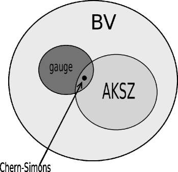
Figure 2: A primitive illustration on the structure of BV space. Chern-Simons theory can be obtained both from the BV formalism for gauge theories and from the reduction of AKSZ version of Chern-Simons.

The largest circle is the whole space of BV theories which we do not discuss in the present paper. One subclass of this space is BV for gauge theories, another one - AKSZ-type theories. In the intersection of these two subclasses the BV version of Chern-Simons is located.

The main issue of this section is to introduce some terminology, which is probably not common, but is widely used for the following discussion. In the next chapters we will demonstrate that a large class of AKSZ theories and even gauge theories can be obtained as effective BV actions from $S^{Fund}$ of (1).

3 Quantum calculations.

In this chapter we explain how one should conduct Feynman diagram calculations in BV integral (8) starting from the action $S^{Fund}$ of (1). Since operator $Q_{B}$ is nilpotent, it is clear that the action (1) has a large gauge freedom. This freedom is to be fixed by the choice of certain lagrangian sub-manifold in the integral (8) providing a well defined diagrammatic expansion for $S^{eff}$. Since initial action (1) contains Grassmann variables in the definition of fields, the diagram expansion of integral (8) terminates at some point, leaving only finite number of diagrams. These diagrams can be summed up explicitly into a very simple effective action, which under certain conditions represents some interesting theories.

The fields in the action (1) belong to the spaces $O[\theta_{\alpha}\ \!,\ \!\lambda_{\alpha}\ |\ f^{\mu}(\lambda)]\otimes Func(x)\otimes T(\mathfrak{g})$ and $O[\theta_{\alpha}\ \!,\ \!\lambda_{\alpha}\ |\ f^{\mu}(\lambda)]^{\ast}\otimes Func(x)\otimes T(\mathfrak{g})$. For the discussion in this section we omit factors $Func(x)$ and $T(\mathfrak{g})$, since they are inessential. The only relevant information is how the fields depend on $\lambda$ and $\theta$.

Expand the fields $\mathcal{A}$ and $\mathcal{P}$ in the action (1) in the classical and quantum parts $\mathcal{A}\ =\ \mathsf{A}\ +\ a$ and $\mathcal{P}\ =\ \mathsf{P}\ +\ p$, where classical fields $\mathsf{A}$ and $\mathsf{P}$ are chosen to take value in the space of cohomologies $\mathcal{H}(Q)$ of the operator $Q=\lambda_{\alpha}\frac{\partial}{\partial\theta_{\alpha}}$ which is the first term in (2), and quantum fields $a$ and $p$ are from the orthogonal complement to $\mathcal{H}(Q)$. Along these fields we do the integration. Then, the action (1) can be rewritten as

$$\begin{split}S^{Fund}(\mathsf{P}+p,\mathsf{A}+a)\ =\ \int\ STr\bigg{(}<p,Qa>\ +\ <\mathsf{P},\Phi a>\ +\ <\mathsf{P},\Phi\mathsf{A}>\ +\ <p,\Phi\mathsf{A}>\ +\\ +\ <p,\Phi a>\ +\ g<(\mathsf{P}+p),(\mathsf{A}+a)^{2}>\bigg{)}\end{split}$$ (21)

Since external fields $\mathsf{A}$ and $\mathsf{P}$ belong to the representatives of $\mathcal{H}(Q)$, the terms $<\mathsf{P},\ Q\mathsf{A}>$, $<\mathsf{P},\ Qa>$, $<p,\ Q\mathsf{A}>$ are equal to zero. It is straightforward to extract vertices from this action. They are:

Figure 3: All the vertices in the theory (21).

In these diagrams solid lines represent external fields. Wavy lines stand for the propagating quantum field. Each line is provided with the arrow sign which notifies whether this line belongs to a field ($\mathcal{A}$) or an antifield ($\mathcal{P}$) of BV formalism. For each field the arrow points into the diagram, for each antifield the arrow points out of the diagram. Each 3-valent vertex contributes a factor of $g$ - the coupling constant.

The first term in (21) is responsible for the propagator of the quantum field. Since operator $Q$ is nilpotent it has a large number of zero modes. To eliminate them consider the following construction. Define the space $V$ as a complement of $\mathcal{H}(Q)$ in $O[\theta_{\alpha}\ \!,\ \!\lambda_{\alpha}\ |\ f^{\mu}(\lambda)]$

$$O[\theta_{\alpha}\ \!,\ \!\lambda_{\alpha}\ |\ f^{\mu}(\lambda)]=\ \mathcal{H}(Q)\ \oplus\ V$$

There is a subspace $\mathcal{C}$ in $V$ of all closed forms which are exact ($\mathcal{C}\subset V$). Choose a basis elements $c_{\alpha}\in\mathcal{C}$, then

$$c_{\alpha}\ =\ Q(b_{\alpha})$$ (22)

In this expression, the elements $b_{\alpha}$ are defined modulo $Q$-exact expressions, remaining the ambiguity in the choice of $b_{\alpha}$. Define the operator $K$ as

$${\begin{array}[]{c}Kc_{\alpha}\ =\ b_{\alpha}\\ Kb_{\alpha}\ =\ 0\end{array}}$$ (23)

This operator maps each element $c_{\alpha}$ to certain element $b_{\alpha}$ breaking the ambiguity of (22). From (22) and (23) it is obvious that $\{K,\ Q\}\ =\ 1$ on the space spanned by $c_{\alpha}$ and $b_{\alpha}$. It is straightforward to check that this space coincides with $V$. Indeed, for arbitrary element $v\in V$, the element $Qv$ is $Q$-closed. Hence, $Qv\ =\ x_{\alpha}c_{\alpha}$ with some coefficients $x_{\alpha}$. Thus, the element $v$ can be represented as

$$v\ =\ x_{\alpha}b_{\alpha}\ +\ y_{\alpha}c_{\alpha}$$ (24)

where $y_{\alpha}$ are some coefficients.

Conducting evaluation of the integral (8) with the action (21) we have already removed part of zero modes from the kinetic term, absorbing them into external fields $\mathsf{P}$ and $\mathsf{A}$. The point is that some of zero modes still survived, because the integral is over the space $V$ which has a sub-space $\mathcal{C}\subset V$ of closed forms. Thus to determine the propagator of quantum field we should remove this ambiguity also. From (24) it is clear that demanding $Kv\ =\ 0$ kills all the terms proportional to $c_{\alpha}$, removing the remnant of zero modes. Thus, the integration in (8) should be restricted by the condition

$${\begin{array}[]{c}Ka\ =\ 0\\ pK\ =\ 0\end{array}}$$ (25)

The only question is whether this condition is a choice of lagrangian sub-manifold or not. The answer to this question is positive. Since $\{K,\ Q\}\ =\ 1$ in the space $V$, both $Q$ and $K$ have no cohomologies in this space. Hence $Ka\ =\ 0$ implies $a\ =\ Kw$ for some element $w$ and

$$\int Tr<\delta p\ ,\ \delta a>\ =\ \int Tr<\delta p\ ,\ K\delta w>\ =\ \int Tr<\delta(pK)\ ,\ \delta w>\ =\ 0$$ (26)

which is the definition of lagrangian sub-manifold (see footnote 3).

Now the integral (8) can be rewritten as

$$e^{-S^{eff}(\mathsf{P},\mathsf{A})}\ =\ \int\limits_{\begin{array}[]{c}Ka=0\\ pK=0\end{array}}\!\!\!{D}p{D}a\ e^{-S^{Fund}(\mathsf{P}+p,\ \mathsf{A}+a)}$$ (27)

This is BV integral, providing $S^{Fund}$ is BV action and (25) determines a lagrangian sub-manifold. Hence $S^{eff}(\mathsf{P},\mathsf{A})$ is again BV action for some theory. Explicit expression for $S^{eff}(\mathsf{P},\mathsf{A})$ is encoded in the choice of background fields $\mathsf{P,A}$, hence in cohomologies of operator $Q$. These cohomologies for an arbitrary set of constraints $f^{\mu}(\lambda)$ will be calculated in the next section.

4 Calculation of Cohomologies

In this chapter we present the general procedure, which allows to find all cohomologies of $Q$-operator in the space $O[\theta_{\alpha}\ \!,\ \!\lambda_{\alpha}\ |\ f^{\mu}(\lambda)]$. This result, to the best of our knowledge is new. Subsection 4.1 contains the general idea, subsection 4.2 - the brute force proof of the theorem (4.1).

4.1 Procedure

The space of complex $O[\theta_{\alpha}\ \!,\ \!\lambda_{\alpha}\ |\ f^{\mu}(\lambda)]$ is defined by the set of quadratic constraints $f^{\mu}(\lambda)$. The function $G^{(1)\ \mu}(\lambda)$ is called a relation if

$$\sum\limits_{\mu=1}^{N}\ \ G^{(1)\ \mu}(\lambda)\ f_{\mu}(\lambda)\ =\ 0$$ (28)

The meaning of superscript $(1)$ will be defined below. From the definition it is clear that multiplying relation $G^{(1)\ \mu}$ by an arbitrary element of the ring $C[\lambda]$ of polynomials in $\lambda_{\alpha}$, we obtain again a relation. Hence, the space of functions $G^{(1)\ \mu}$, satisfying equation (28) forms a module over the ring $C[\lambda]$. The minimal set of functions $G_{A}^{(1)\ \mu}(\lambda)$ (index $A$ enumerates different functions) which generates the whole module via multiplication by the elements of $C[\lambda]$ is called the fundamental system of relations. An arbitrary relation $G^{(1)\ \mu}(\lambda)$ can be obtained from the fundamental system of relations $G_{A}^{(1)\ \mu}(\lambda)$ as the sum $G^{(1)\ \mu}(\lambda)\ =\ K^{A}(\lambda)G_{A}^{(1)\ \mu}(\lambda)$, where $K^{A}(\lambda)$ is some function. In case $K^{A}(\lambda)\ =\ const$, relation $G^{(1)\ \mu}(\lambda)$ is fundamental. If $K^{A}(\lambda)\ \neq\ const$ relation $G^{(1)\ \mu}(\lambda)$ is not fundamental.

Relation $G^{(1)\ \mu}(\lambda)$ is called trivial if it belongs to the ideal $I_{f}$ ( if its coefficients are proportional to $f^{\mu}(\lambda)$ ).

The following example illustrates the definitions given above.

Example Consider the set of quadrics $f_{1}=\lambda_{1}^{2}\ \ \ f_{2}=\lambda_{1}\lambda_{2}$. Relation $G^{\mu}(\lambda)\ \$ ($G^{\ 1}f_{1}+G^{\ 2}f_{2}=0$) is trivial for

$$G^{\ 1}=\lambda_{1}\lambda_{2}\ \ \ \ G^{\ 2}=-\lambda_{1}^{2}$$

because its coefficients are proportional to quadrics.

Relation $L^{\mu}(\lambda)$:

$$L^{\ 1}=\lambda_{2}\ \ \ \ \ L^{\ 2}=-\lambda_{1}$$

is non-trivial.

In this particular example relation $L^{\mu}(\lambda)$ is fundamental, while $G^{\mu}(\lambda)$ is not fundamental (it is obtained from multiplication of $L^{\mu}(\lambda)$ by $\lambda_{1}$). In general situation this is not true. Whether relation is trivial or not has nothing to do with the fact whether it is fundamental or not. The fundamental system of relations for this set of quadrics $f^{\mu}(\lambda)$ consists of one relation $G_{1}^{(1)\ \mu}$ which coincides with $L^{\mu}(\lambda)$  $(\ G_{1}^{(1)\ \mu}\ =\ L^{\mu}(\lambda)\ )$.

Suppose the fundamental system of relations is found. It is given by the set of basis elements enumerated by the index $A$. Define the second-level relations as "relations for relations":

$$\sum\limits_{A}\ \ G^{(2)\ A}(\lambda)\ G_{A}^{(1)\ \mu}(\lambda)\ =\ 0$$ (29)

Now the meaning of the superscripts $(1)$ and $(2)$ is obvious. Equation (29) should be valid for arbitrary value of index $\mu$. Such secondary relations again form a module. It is possible to find a basis in this module - the fundamental system of relations at the second level. These relations are $G_{B}^{(2)\ A}(\lambda)$, where index $B$ enumerates the fundamental relations at the second level. Conducting the same manipulations, we define $G_{C}^{(n)\ D}(\lambda)$ at the n-th level. The following theorem can be proved:
Theorem Suppose the fundamental set $G_{A}^{(n)\ B}(\lambda)$ is found. All cohomologies $\mathcal{H}(Q\ ,\ O)$ of the $Q$-operator in the space $O[\theta_{\alpha}\ \!,\ \!\lambda_{\alpha}\ |\ f^{\mu}(\lambda)]$ are given by:

$$1$$

$$\widetilde{D}f^{\mu}(\lambda)$$

$$\widetilde{D}\Big{(}\widetilde{D}G_{A_{1}}^{(1)\ \mu}(\lambda)\ f_{\mu}(\lambda)\Big{)}$$ (30)

$$\widetilde{D}\Bigg{(}\widetilde{D}\Big{(}\widetilde{D}G_{A_{2}}^{(2)\ A_{1}}(\lambda)\ G_{A_{1}}^{(1)\ \mu}(\lambda)\Big{)}\ f_{\mu}(\lambda)\Bigg{)}$$

$$...........................................................$$

We assume summation over repeated indices. To define operator $\widetilde{D}$ consider first nilpotent operator $D$:

$$D=\theta_{a}\frac{\partial}{\partial\lambda_{a}}$$

It is straightforward to check that anticommutator

$$\{Q\ ,\ D\}\ =\ \theta_{a}\frac{\partial}{\partial\theta_{a}}\ +\ \lambda_{a}\frac{\partial}{\partial\lambda_{a}}\ =\ deg(\theta)+deg(\lambda)\ =\ deg$$ (31)

is the degree operator. Define operator $\widetilde{D}$ as $\widetilde{D}\ =\ \frac{1}{deg}D$. Such operator can be applied to all functions except constants. In the tower (4.1) it is applied to functions $f^{\mu}(\lambda)$, which are quadratic in $\lambda_{\alpha}$ and to the basis functions of fundamental system of relations. Such functions should be at least linear in $\lambda_{\alpha}$. (We are not interested in constant relations because they are simple linear redefinitions of basis elements. Such redefinitions do not affect the cohomologies.) Using this definition equation (31) can be rewritten as

$$\{Q\ ,\ \widetilde{D}\}\ =\ 1$$ (32)

The cohomologies (4.1) are written in such a way, that each new line gives one extra degree of $\theta$. Since $\theta$ are Grassmann variables and the number of them is limited in the space $O[\theta_{\alpha}\ \!,\ \!\lambda_{\alpha}\ |\ f^{\mu}(\lambda)]$, the tower (4.1) stops at some point. Hence the number of representatives is finite.

4.2 Proof of the theorem

The proof of the theorem goes in 3 steps: firstly we check that expressions (4.1) are closed, secondly that they are not exact, finally that (4.1) gives all cohomologies. The first two steps are presented in this section, while the third one is given in the appendix. In this section we denote by equality sign $=$ the equality between the polynomials in the ring $C[\lambda,\theta]$, while by $\sim$ sign we mean the equality modulo factorization over the ideal $I_{f}$.

4.2.1 Closeness

1 is obviously $Q$-closed. Applying $Q$ to second representative $\widetilde{D}f^{\mu}$, one can get:

$$Q\widetilde{D}f^{\mu}\ =\ \{Q,\widetilde{D}\}f^{\mu}\ -\ \widetilde{D}Qf^{\mu}\ =\ f^{\mu}\ \sim\ 0$$ (33)

In the second term of the first equality the fact that $f^{\mu}$ does not depend on $\theta$, hence $Qf^{\mu}=0$ is used. We also take into account equation (32). In the last equality we use the fact that we are working in the space $O[\theta_{\alpha}\ \!,\ \!\lambda_{\alpha}\ |\ f^{\mu}(\lambda)]$, hence all elements from the ideal $I_{f}$ (proportional to $f^{\mu}$) are equivalent to $0$. Applying $Q$ to the next term,

$$Q\Bigg{[}\widetilde{D}\Big{(}\widetilde{D}G_{A}^{(1)\ \mu}\ f_{\mu}\Big{)}\Bigg{]}\ =\ \widetilde{D}G_{A}^{(1)\ \mu}f_{\mu}\ -\ \widetilde{D}\Big{(}Q\widetilde{D}G_{A}^{(1)\ \mu}\ f_{\mu}\Big{)}\ =\ \widetilde{D}G_{A}^{(1)\ \mu}f_{\mu}\ -\ \widetilde{D}\Big{(}G_{A}^{(1)\ \mu}f_{\mu}\Big{)}\ =\ \widetilde{D}G_{A}^{(1)\ \mu}f_{\mu}\ \sim\ 0$$

In the first equality we use equation (32), Leibniz identity for $Q$ and the fact that $f^{\mu}$ do not depend on $\theta$, hence $Qf^{\mu}\ =\ 0$. In the second equality we again explore equation (32) and $QG_{A}^{(1)\ \mu}\ =\ 0$. In the next equality we use that $G_{A}^{(1)\ \mu}\ f_{\mu}\ =\ 0$ is a relation. Last equivalence sign is the factorization procedure.

The closeness of other terms in (4.1) can be proved in a similar way.

4.2.2 Non-Exactness

1 is obviously not Q exact. Below we present an illustration of proof that all other terms in (4.1) are not exact. The proof is universal for all the terms in the tower (4.1). We take the third term to show how it works. Suppose it is exact. Since we are working in a coset space this means(we omit index $A_{1}$)

$$\widetilde{D}\Big{(}\widetilde{D}G^{(1)\ \mu}(\lambda)\ f_{\mu}(\lambda)\Big{)}\ =\ Q(M)\ +\ c^{\mu}(\lambda,\theta^{2})f_{\mu}$$

Here $c^{\mu}(\lambda,\theta^{2})$ are some functions quadratic in $\theta^{\alpha}$ (this degree is dictated by the degree in $\theta^{\alpha}$ of the l.h.s.). Applying operator $Q$ to this relation, one can get

$$\widetilde{D}G^{(1)\ \mu}f_{\mu}\ -\ \widetilde{D}\Big{(}Q\widetilde{D}G^{(1)\ \mu}\ f_{\mu}\Big{)}\ =\ Qc^{\mu}(\lambda,\theta^{2})f_{\mu}$$

Using equation (32) one can show that the second term in the l.h.s. vanishes. Hence, there is a relation on $f^{\mu}(\lambda)$

$$\big{[}\widetilde{D}G^{(1)\ \mu}\ -\ Qc^{\mu}(\lambda,\theta^{2})\Big{]}f_{\mu}\ =\ 0$$

Each relation can be expanded in the basis of fundamental relations

$$\widetilde{D}G^{(1)\ \mu}\ -\ Qc^{\mu}(\lambda,\theta^{2})\ =\ K^{A}(\lambda,\theta)G_{A}^{(1)\ \mu}$$

were $K^{A}(\lambda,\theta)$ is linear in $\theta^{\alpha}$. Applying to the both sides operator $Q$, one can get

$$G^{(1)\ \mu}\ =\ Q\Big{(}K^{A}(\lambda,\theta)\Big{)}G_{A}^{(1)\ \mu}$$

Since $K^{A}(\lambda,\theta)$ is linear in $\theta^{\alpha}$, from this expression it is clear that $G^{(1)\ \mu}$ is at least one degree in $\lambda^{\alpha}$ higher than the fundamental system of relations $G_{A}^{(1)\ \mu}$, hence is not fundamental. This completes the proof that the third element in (4.1) is not exact. The proof for all other terms is analogous.

Thus, we have checked that all the expressions which are written in (4.1) are indeed cohomologies. The only question remains whether we have found all of them.

4.2.3 Completeness

The proof that the set (4.1) is complete is presented in the appendix.

Concluding this section, we introduce one more definition.
Definition of "regular" and "singular" quadrics. Suppose the set of quadrics $f^{\mu}(\lambda)$ is chosen in such a way, that all relations, used to generate the tower of cohomologies (4.1) are trivial (according to the definition above the example in section 4.1). In this case we call the set $f^{\mu}(\lambda)$ - the "regular" system of quadrics. In case there is at least one non-trivial relation, the system $f^{\mu}(\lambda)$ is called "singular".

From the point of the discussed construction "regular" quadrics are the simplest systems. In the next section it will be demonstrated that in case of "regular" system the algebra of cohomologies $\mathcal{H}(Q)$ is isomorphic to the exterior algebra $\Lambda^{\bullet}\{\widetilde{D}f_{1},.....,\widetilde{D}f_{N}\}$ of the generators $\widetilde{D}f_{1},.....,\widetilde{D}f_{N}$. Hence, the only information which is inherited by this algebra from the quadrics $f^{\mu}(\lambda)$ is that the system is "regular" and that there are $N$ quadrics. All the information about particular structure ( $\lambda_{\alpha}$-dependence ) of quadrics is irrelevant for $\mathcal{H}(Q)$ and hence for the effective action. Thus, effective action for arbitrary "regular" system of quadrics is universal, i.e. does not depend on the particular, probably very complicated, expressions for $f^{\mu}(\lambda)$. It happens that this universal effective action is nothing but BV version of AKSZ-Chern-Simons theory (19).

5 AKSZ version of Chern-Simons as effective BV theory

We start from one of the simplest examples. Consider the space $O[\theta_{\alpha}\ \!,\ \!\lambda_{\alpha}\ |\ f^{\mu}(\lambda)]$, generated by three $\theta$, three $\lambda$ ($\alpha=1,2,3$) and the set of quadratic constraints

$$f_{1}=\frac{\lambda_{1}^{2}}{2}$$

$$f_{2}=\frac{\lambda_{2}^{2}}{2}$$ (34)

$$f_{3}=\frac{\lambda_{3}^{2}}{2}$$

5.1 Calculation of Cohomologies

We begin analysis of this example from calculation of all cohomologies $\mathcal{H}(Q,\ O)$, according to (4.1). First of all one should determine the fundamental set of relations (28) at the first level $G^{(1)\ \!\mu}_{A}(\lambda)$. These relations are:

$$\begin{array}[]{ccccccccccc}\lambda_{3}^{2}f_{2}&-&\lambda_{2}^{2}f_{3}&=&0&&G^{(1)}_{1}\ =&\!\!\!(\ \ \ \ 0&\ \ \lambda_{3}^{2}&-\lambda_{2}^{2}\ )&\\ \lambda_{1}^{2}f_{3}&-&\lambda_{3}^{2}f_{1}&=&0&&G^{(1)}_{2}\ =&(\ \ -\lambda_{3}^{2}&\ \ 0&\ \ \lambda_{1}^{2}\ )&\\ \lambda_{2}^{2}f_{1}&-&\lambda_{1}^{2}f_{2}&=&0&&G^{(1)}_{3}\ =&(\ \ \ \lambda_{2}^{2}&\ \ -\lambda_{1}^{2}&\ \ \ 0\ \ )&\\ \end{array}$$ (35)

There is only one second-level relation $G^{(2)\ \!\!A}_{1}(\lambda)$:

$$\lambda_{1}^{2}G^{(1)}_{1}\ +\ \lambda_{2}^{2}G^{(1)}_{2}\ +\ \lambda_{3}^{2}G^{(1)}_{3}\ =\ 0$$ (36)

written in the basis $(f_{1},\ f_{2}\ f_{3})$. At this point the tower of relations stops. All found relations $G^{(1)}$ and $G^{(2)}$ are trivial, because their coefficients are proportional to $f^{\mu}(\lambda)$, hence the set (5) is "regular", according to the definition in the end of the previous section. Now we can write down all cohomologies $\mathcal{H}(Q,\ O)$ in this example. They are obtained (4.1) by applying operator $\widetilde{D}$ to all fundamental relations. The result is:

$$\mathcal{H}(Q,\ O)\ =\ \left({\begin{array}[]{ccc}&1&\\ \lambda_{1}\theta_{1}&\lambda_{2}\theta_{2}&\lambda_{3}\theta_{3}\\ \lambda_{1}\lambda_{2}\theta_{1}\theta_{2}&\lambda_{1}\lambda_{3}\theta_{1}\theta_{3}&\lambda_{2}\lambda_{3}\theta_{2}\theta_{3}\\ &\lambda_{1}\lambda_{2}\lambda_{3}\theta_{1}\theta_{2}\theta_{3}&\\ \end{array}}\right)$$ (37)

5.2 An Illustrative Example on Diagram Evaluation

Second step is evaluation of effective action (27) by means of diagram expansion in (21). To begin with we present a simple example calculating the 4-point amplitude presented in figure 4.

As we explain below, this diagram is forbidden (is equal to zero) for the regular set(5). It is presented here only for illustrative purposes, clarifying the whole procedure of diagram evaluation.

According to discussion after figure 3 external lines stand for the background fields $\mathsf{P,A}\in\mathcal{H}(Q,O)\otimes Func(x)\otimes T(\mathfrak{g})$. In this particular example there are three in-lines, corresponding to a field $\mathsf{A}$, and one out-line, corresponding to an antifield $\mathsf{P}$.

Figure 4: 4-point amplitude.

It happens that this is the general feature of arbitrary tree diagram in the theory (21). Each connected diagram (only connected diagrams are relevant for calculation of effective action) can have many in-lines but only one out-line. This is illustrated in the figure 5.

Figure 5: A tree diagram in the theory (21).

Due to this fact, the diagram technique is non-trivial only at the tree level and in 1-loop. All higher loops are absent. Indeed, the only possibility to organize a loop is to close the out-line onto one of the in-lines, like in the figure 6.

Figure 6: Closing a tree into one loop.

The resulting diagram has only one loop and only in-lines, prohibiting formation of an another loop.

Now we are coming back to evaluation of the diagram in figure 4. To find this amplitude, we need expression for the propagator. To obtain it, introduce the sources for the quantum fields $a$ and $p$.

$$\begin{split}\int\limits_{\small\begin{array}[]{c}Ka=0\\ pK=0\end{array}}DpDa\ e^{-(pQa\ +\ pJ_{p}\ +\ J_{a}a)}\ \ =\ \ \int\limits_{\small\begin{array}[]{c}Ka=0\\ pK=0\end{array}}DpDa\ e^{-(pQa\ +\ pJ_{p}\ +\ J_{a}\{K,Q\}a)}\ \ =\ \ \ \ \ \ \ \ \ \\ =\!\!\!\int\limits_{\small\begin{array}[]{c}Ka=0\\ pK=0\end{array}}DpDa\ e^{-(p\ +\ J_{a}K)(Qa\ +\ J_{p})\ +\ J_{a}KJ_{p}}\ \ =\int\limits_{\small\begin{array}[]{c}Ka=0\\ pK=0\end{array}}DpDa\ e^{-(p\ +\ J_{a}K)Q(a\ +\ KJ_{p})+\ J_{a}KJ_{p}}\ \ \sim\ \ {\Huge e^{J_{a}KJ_{p}}}\end{split}$$

Here in the first equality we inserted $\{K\ ,\ Q\}\ =\ 1$ in the space $V$ ( see discussion after (25) ). In the second equality we explored the definition of lagrangian sub-manifold $Ka\ =\ 0$ and extracted the total square. In the next equality we again inserted $\{K\ ,\ Q\}\ =\ 1$ in front of the source $J_{p}$ and used that $(p\ +\ J_{a}K)K\ =\ 0$ due to $K^{2}=0$ and the definition of lagrangian sub-manifold. The last proportionality sign is obtained after the integration over $a$ and $p$. One can shift the integration variables by the terms $J_{a}K$ and $KJ_{p}$ because this shift is along the integration domain. Thus the propagator in (21) is given by $K$.

To find the amplitude in figure 4 one should first multiply two representatives $\mathsf{A_{1},A_{2}}\in\mathcal{H}(Q)\otimes Func(x)\otimes T(\mathfrak{g})$ in the left vertex. Since both expressions are closed, the result is the sum of a representative $\mathcal{H}(Q)$ and an exact expression

$$g\mathsf{A_{1}\cdot A_{2}}\ =\ h\ +\ Q(\omega)$$

where $h\in\mathcal{H}(Q)$ and $K\omega\ =\ 0$. At the next step one should apply to this result operator $K$, which is responsible for propagating quantum field. Strictly speaking operator $K$ is defined only on the space $V$ and can not be applied to $\mathcal{H}(Q)$. However we extend the domain of $K$ and define this action as $K\mathcal{H}(Q)\ =\ 0$. Thus, due to (23), the result is

$$K(g\mathsf{A_{1}\cdot A_{2}})\ =\ \omega$$

To finish evaluation of the diagram in figure 4, one should multiply the last in-line $\mathsf{A_{3}}$ by $\omega$ and project the result onto $\mathcal{H}(Q)$. This is done by calculation of the canonical pairing $<\mathsf{P},\ g\mathsf{A}_{3}\cdot\omega>\ =\ <\mathsf{P},\ g\mathsf{A}_{3}\cdot K(g\mathsf{A}_{1}\cdot\mathsf{A}_{2})>$ from the introduction. Such projection is non-zero only if some part of expression $g^{2}\mathsf{A_{3}}\cdot K(\mathsf{A_{1}\cdot A_{2}})$ is a representative of $\mathcal{H}(Q)$. Otherwise this amplitude is equal to zero.

Since the theory (1) contains Grassmann variables it is important to fix convention of how one should multiply the fields in each 3-valent vertex. We use the clockwise rule for that. This means that one should multiply the fields in the clockwise direction, starting from the out-line. This convention was illustrated in the example above: in the first vertex the order of multiplication is $\mathsf{A_{1}}\cdot\mathsf{A_{2}}$ ( not $\mathsf{A_{2}}\cdot\mathsf{A_{1}}$ ), in the second vertex $\mathsf{A_{3}}\cdot\omega$ (not $\omega\cdot\mathsf{A_{3}}$).

By this remark we conclude our illustrative example with the 4-point amplitude and switch to evaluation of effective action for the regular set (5). In this example all representatives of $\mathcal{H}(Q)$ have remarkable feature (see explicit expressions (37) ): $\#\lambda=\#\theta$ (number of $\lambda$ $=$ number of $\theta$). Propagator $K\ =\ Q^{-1}\ =\ [\lambda_{\alpha}\frac{\partial}{\partial\theta_{\alpha}}]^{-1}$ decreases $\#\lambda$ by $1$ and increases $\#\theta$ by $1$, violating $\#\lambda\ =\ \#\theta$. Hence all the tree diagrams with propagating quantum field (like the one in the figure 4) are forbidden (the canonical pairing is equal to zero). We have explained above that diagram technique in the theory (21) is non-trivial only in one loop. It is obvious that for particular example of operator $Q\ =\ \lambda_{\alpha}\frac{\partial}{\partial\theta_{\alpha}}$ in the kinetic term even 1-loop diagrams are absent. One of several arguments for this is that the only possible loop diagram is the one presented in the figure (7).

Figure 7: The only possible 1-loop diagram in the theory (21).

This diagram can have only in-lines. Since each propagator $Q^{-1}$ increases the number of $\theta$ by $1$, in-lines should contribute some negative power of $\theta$, to have a chance to close the loop. But there are no fields with negative degree of $\theta$. Hence there are no loop diagrams at all.

We conclude that in this particular example there are no loop diagrams and there are no non-trivial tree diagrams, having propagating quantum field. Hence, the only relevant diagrams are those depicted in the figure 8.

5.3 Calculation of Effective Action for the "Regular" Set (5)

A convenient way of evaluation for these diagrams is the introduction of the superfield

$$\mathsf{A}\ \ \ \ = c\ \ \ \ +\ \ \ \lambda_{1}\theta_{1}A_{1}\ +\ \lambda_{2}\theta_{2}A_{2}\ +\ \lambda_{3}\theta_{3}A_{3}\ +\$$

$$+\ \lambda_{2}\lambda_{3}\theta_{2}\theta_{3}A_{1}^{\ast}\ -\ \lambda_{1}\lambda_{3}\theta_{1}\theta_{3}A_{2}^{\ast}\ +\ \lambda_{1}\lambda_{2}\theta_{1}\theta_{2}A_{3}^{\ast}\ +\ \!\!\!\!\lambda_{1}\lambda_{2}\lambda_{3}\theta_{1}\theta_{2}\theta_{3}\ c^{\ast}$$

In this superfield all representatives of $\mathcal{H}(Q)$ found in (37) are included. Letters $c,A_{\mu},A^{\ast}_{\mu},c^{\ast}\ \in Func(x)\otimes T(\mathfrak{g})$ stand for the fields which will finally form effective action. Minus sign in front of $\lambda_{1}\lambda_{3}\theta_{1}\theta_{3}$ is chosen for the future convenience. From the definition of the superfield it is clear that representatives of $\mathcal{H}(Q)$ play the role of polarizations for the fields $c$, $A_{\mu}$, $A^{\ast}_{\mu}$, $c^{\ast}$. We would like to emphasize that though in section 2 we used notation $A^{\ast}$ for BV antifield to a field $A$, in the superfield (5.3) the field $A^{\ast}_{\mu}$ is not an antifield to $A_{\mu}$ and $c^{\ast}$ is not an antifield to $c$. They will become such fields only after $Z_{2}$ reduction discussed in the section 2. While at the present moment the antifields (see (5.3) below) are denoted by tilde-sign, like $\widetilde{c}$, $\widetilde{A}_{\mu}$, etc.

Figure 8: Relevant diagrams for AKSZ-Chern-Simons theory, produced from the quadrics (5).

To calculate the first diagram in the figure 8 we should apply operator $\Phi$

$$\Phi\ =\ \theta_{\alpha}\frac{\partial f^{\mu}}{\partial\lambda_{\alpha}}\partial_{\mu}\ =\ \lambda_{1}\theta_{1}\partial_{1}\ +\ \lambda_{2}\theta_{2}\partial_{2}\ +\ \lambda_{3}\theta_{3}\partial_{3}$$

to the superfield $\mathsf{A}$, which stands for the in-line in this diagram, and project the result onto cohomologies $\mathcal{H}(Q)$. This is done by calculation of the canonical pairing $<\ ,\ >$ with the anti-superfield

$$\mathsf{P}\ \ \ \ = \widetilde{c}\ \ \ \ -\ \ \ \underline{\lambda_{1}\theta_{1}}\widetilde{A}_{1}\ -\ \underline{\lambda_{2}\theta_{2}}\widetilde{A}_{2}\ -\ \underline{\lambda_{3}\theta_{3}}\widetilde{A}_{3}\ +\$$

$$+\ \underline{\lambda_{2}\lambda_{3}\theta_{2}\theta_{3}}\widetilde{A}^{\ast}_{1}\ -\ \underline{\lambda_{1}\lambda_{3}\theta_{1}\theta_{3}}\widetilde{A}^{\ast}_{2}\ +\ \underline{\lambda_{1}\lambda_{2}\theta_{1}\theta_{2}}\widetilde{A}^{\ast}_{3}\ -\ \!\!\!\!\underline{\lambda_{1}\lambda_{2}\lambda_{3}\theta_{1}\theta_{2}\theta_{3}}\ \widetilde{c}^{\ast}$$

For instance, take the field $\lambda_{1}\theta_{1}A_{1}$. One should apply operator $\Phi$ to it:

$$\Phi\big{(}\lambda_{1}\theta_{1}A_{1}\big{)}\ =\ \lambda_{1}\lambda_{2}\theta_{2}\theta_{1}\partial_{2}A_{1}\ +\ \lambda_{1}\lambda_{3}\theta_{3}\theta_{1}\partial_{3}A_{1}$$

The result of projection onto $\mathcal{H}(Q)$ is given by:

$$\begin{split}<\mathsf{P},\ \lambda_{1}\lambda_{2}\theta_{2}\theta_{1}\partial_{2}A_{1}\ +\ \lambda_{1}\lambda_{3}\theta_{3}\theta_{1}\partial_{3}A_{1}>\ =\ <\underline{\lambda_{1}\lambda_{2}\theta_{1}\theta_{2}}\widetilde{A}^{\ast}_{3},\ \lambda_{1}\lambda_{2}\theta_{2}\theta_{1}\partial_{2}A_{1}>\ +\\ +\ <-\underline{\lambda_{1}\lambda_{3}\theta_{1}\theta_{3}}\widetilde{A}^{\ast}_{2},\ \lambda_{1}\lambda_{3}\theta_{3}\theta_{1}\partial_{3}A_{1}>\ =\ -\widetilde{A}^{\ast}_{3}\partial_{2}A_{1}\ +\ \widetilde{A}^{\ast}_{2}\partial_{3}A_{1}\end{split}$$

Conducting such manipulations for each component field of the superfield $\mathsf{A}$ one can obtain the first line of the effective action (40). Evaluation of the second diagram of figure 8 goes in a similar way: one should multiply two superfields $\mathsf{A}$ corresponding to the in-lines and project the result onto the out-line - the superfields $\mathsf{P}$. The sum of contributions of these two diagrams is given by

$$\begin{split}S^{eff}\ \ \ =\ \ \ \int d^{3}x\ STr\Big{(}\ -\ \widetilde{A}_{\mu}\partial_{\mu}c\ \ -\ \ \widetilde{c}^{\ast}\partial_{\mu}A_{\mu}^{\ast}\ \ +\ \ \varepsilon^{\mu\nu\lambda}\widetilde{A}^{\ast}_{\mu}\partial_{\nu}A_{\lambda}\ \ +\ \ \ \ \ \ \ \ \ \ \ \\ +\ g\varepsilon^{\mu\nu\lambda}\widetilde{A}^{\ast}_{\mu}A_{\nu}A_{\lambda}\ +\ g\widetilde{c}cc\ +\ g\widetilde{A}_{\mu}[c,\ A_{\mu}]\ +\ g\widetilde{A}^{\ast}_{\mu}\{c,\ A_{\mu}^{\ast}\}\ +\ g\widetilde{c}^{\ast}\ [c,\ c^{\ast}]\ +\ g\widetilde{c}^{\ast}\ [A_{\mu}^{\ast},\ A_{\mu}]\Big{)}\end{split}$$ (40)

Since we have started from BV action (21) and integrated over the lagrangian sub-manifold (25), effective action should be again BV version of some theory. It happens that (40) is nothing but AKSZ-type BV action for Chern-Simons theory (19) (see for example [16]). To see this, one should expand the fields $\Psi\ =\ \Psi^{(0)}\ +\ \Psi^{(1)}\ +\ \Psi^{(2)}\ +\ \Psi^{(3)}$ and $\Psi^{\ast}\ =\ \Psi^{\ast(0)}\ +\ \Psi^{\ast(1)}\ +\ \Psi^{\ast(2)}\ +\ \Psi^{\ast(3)}$ in the action (19). The result is

$$\begin{split}S^{AKSZ-CS}\ =\ \int STr\Big{(}\Psi^{\ast(0)}d\Psi^{(2)}\ +\ \Psi^{\ast(2)}d\Psi^{(0)}\ +\ \Psi^{\ast(1)}d\Psi^{(1)}\ +\ g\Psi^{\ast(3)}\Psi^{(0)}\Psi^{(0)}\ +\ g\Psi^{\ast(2)}\{\Psi^{(0)},\Psi^{(1)}\}\ +\ \\ +\ g\Psi^{\ast(1)}\{\Psi^{(0)},\Psi^{(2)}\}\ +\ g\Psi^{\ast(0)}\{\Psi^{(0)},\Psi^{(3)}\}\ +\ g\Psi^{\ast(1)}\Psi^{(1)}\Psi^{(1)}\ +\ g\Psi^{\ast(0)}\{\Psi^{(1)},\Psi^{(2)}\}\Big{)}\end{split}$$ (41)

Action (41) reproduces effective action (40) under the identification

$${\begin{array}[]{cccc}\!\!\!\!\Psi^{(0)}\ =\ c&\ \ \ \Psi^{(1)}\ =\ dx^{\mu}A_{\mu}&\ \ \ \Psi^{(2)}\ =\ \frac{1}{2}\ dx^{\mu}\wedge dx^{\nu}\ \varepsilon_{\mu\nu\lambda}\ A_{\lambda}^{\ast}&\ \ \ \Psi^{(3)}\ =\ \frac{1}{6}\ dx^{\mu}\wedge dx^{\nu}\wedge dx^{\lambda}\ \varepsilon_{\mu\nu\lambda}\ c^{\ast}\\ \\ \Psi^{\ast(0)}\ =\ \widetilde{c}^{\ast}&\ \ \ \Psi^{\ast(1)}\ =\ dx^{\mu}\widetilde{A}^{\ast}_{\mu}&\ \ \ \Psi^{\ast(2)}\ =\ \frac{1}{2}\ dx^{\mu}\wedge dx^{\nu}\ \varepsilon_{\mu\nu\lambda}\ \widetilde{A}_{\lambda}&\ \ \ \Psi^{\ast(3)}\ =\ \frac{1}{6}\ dx^{\mu}\wedge dx^{\nu}\wedge dx^{\lambda}\ \varepsilon_{\mu\nu\lambda}\ \widetilde{c}\end{array}}$$

In this calculation one should take into account the parities of the fields:

even odd

$$A_{\mu}\ \ c^{\ast}\ \ \ \ \widetilde{A}_{\mu}^{\ast}\ \ \widetilde{c}$$

and that odd fields anticommute with the generators of exterior algebra $dx^{\mu}$. Hence, in most of terms in (41) anticommutators transform into commutators.

Thus, we have demonstrated that AKSZ version of Chern-Simons theory can be obtained as effective action from the theory (1). It is instructive to note that the action (40) transforms into normal BV action for Chern-Simons gauge theory under the reduction over half of degrees of freedom

$$\begin{array}[]{cc}\widetilde{A}^{\ast}_{\mu}\ =\ A_{\mu}&\widetilde{c}^{\ast}\ =\ c\\ \widetilde{A}_{\mu}\ =\ A_{\mu}^{\ast}&\widetilde{c}\ =\ c^{\ast}\end{array}$$

This $Z_{2}$ reduction was mentioned in the section 2, see also figure 2. It is possible to do such reduction in case the dimension of space-time is odd. After this reduction the action (40) transforms to

$$\begin{split}S^{CS-gauge}\ \ \ =\ \ \ \int d^{3}x\ STr\Big{(}\ -\ 2A^{\ast}_{\mu}\partial_{\mu}c\ +\ 3gA^{\ast}_{\mu}[c,\ A_{\mu}]\ +\ 3g\ \!c^{\ast}cc\ +\ \varepsilon^{\mu\nu\lambda}A_{\mu}\partial_{\nu}A_{\lambda}\ +\ g\varepsilon^{\mu\nu\lambda}A_{\mu}A_{\nu}A_{\lambda}\Big{)}\end{split}$$

which is BV action of Chern-Simons gauge theory under redefinitions $g\longrightarrow\frac{2}{3}g$, $c^{\ast}\longrightarrow\frac{1}{2}c^{\ast}$ and $A_{\mu}^{\ast}\longrightarrow\frac{1}{2}A_{\mu}^{\ast}$. In this action the field $A_{\mu}$ is the gauge field, $A^{\ast}_{\mu}$ is BV anti-gauge field, $c$ is the ghost field and $c^{\ast}$ is BV anti-ghost field.

5.4 Generalization for arbitrary "regular" system of constraints

Thus, we have demonstrated that the theory (40) arises as effective action for particular choice of constraints (5). It happens that this result is in fact more general. The same effective action can be obtained for arbitrary "regular" set of constraints. To see this, note that in case of "regular" quadrics the first-level relations can be written as

$$G^{(1)\ \mu_{1}}\ =\ \varepsilon^{\mu_{1}\mu_{2}}f_{\mu_{2}}$$

where $\varepsilon^{\mu_{1}\mu_{2}}$ is an arbitrary antisymmetric matrix. It is convenient to choose a basis in the space of such matrices. The basis elements are denoted by two indices $\alpha_{1}$ and $\alpha_{2}\ \ \$: $\varepsilon^{\mu_{1}\mu_{2}}_{\alpha_{1}\ \alpha_{2}}$ - the matrix which has $1$ at the intersection of $\alpha_{1}$-th line and $\alpha_{2}$-th column and $-1$ at the $\alpha_{1}$-th column and $\alpha_{2}$-th line. Explicit expression for such matrix is

$$\varepsilon^{\mu_{1}\mu_{2}}_{\alpha_{1}\ \alpha_{2}}\ =\ \big{(}\delta^{\mu_{1}}_{\alpha_{1}}\delta^{\mu_{2}}_{\alpha_{2}}\ -\ \delta^{\mu_{1}}_{\alpha_{2}}\delta^{\mu_{2}}_{\alpha_{1}}\big{)}$$

Thus, in "regular" case the first-level relations are:

$$G^{(1)\ \mu_{1}}_{\alpha_{1}\ \alpha_{2}}\ =\ \big{(}\delta^{\mu_{1}}_{\alpha_{1}}\delta^{\mu_{2}}_{\alpha_{2}}\ -\ \delta^{\mu_{1}}_{\alpha_{2}}\delta^{\mu_{2}}_{\alpha_{1}}\big{)}f_{\mu_{2}}$$

They obviously satisfy $G^{(1)\ \mu_{1}}_{\alpha_{1}\ \alpha_{2}}f_{\mu_{1}}\ =\ 0$. Explicit expressions for the second-level relations are

$$G^{(2)\ \alpha_{1}\ \alpha_{2}}_{\beta_{1}\ \beta_{2}\ \beta_{3}}\ =\ \delta^{\alpha_{1}}_{[\beta_{1}}\delta^{\alpha_{2}}_{\beta_{2}}\delta^{\alpha_{3}}_{\beta_{3}]}\ f_{\alpha_{3}}$$

where one should make antisymmetrization over the indices $\beta_{1}$,$\beta_{2}$,$\beta_{3}$. Expressions for the n-th level relations are

$$G^{(n)\ \ \alpha_{1},.....,\alpha_{n}}_{\ \ \ \ \beta_{1},.....,\beta_{n+1}}\ =\ \delta^{\alpha_{1}}_{[\beta_{1}}.....\delta^{\alpha_{n+1}}_{\beta_{n+1}]}\ f_{\alpha_{n+1}}$$

To extract cohomologies from this system of relations one should apply operator $\widetilde{D}$ to them according to (4.1). Straightforward calculation for the first-level relations gives

$$\widetilde{D}G^{(1)\ \!\beta_{1}}_{\alpha_{1}\ \alpha_{2}}\widetilde{D}f_{\beta_{1}}\ =\ 2\widetilde{D}f_{\alpha_{2}}\widetilde{D}f_{\alpha_{1}}$$

Similar computation for higher-order relations demonstrate that the algebra of cohomologies (4.1) is isomorphic to exterior algebra $\Lambda^{\bullet}\{\widetilde{D}f_{1},.....,\widetilde{D}f_{N}\}$ of anticommuting generators $\widetilde{D}f_{1},.....,\widetilde{D}f_{N}$. Hence, we conclude that for "regular" system of quadrics the algebra of cohomologies is universal and does not depend on explicit expressions of quadrics $f^{\mu}(\lambda)$. The same is true for the effective action. Since $\mathcal{H}(Q)\ =\ \Lambda^{\bullet}\{\widetilde{D}f_{1},.....,\widetilde{D}f_{N}\}$, each representative has $\#\lambda=\#\theta$ (degree of $\lambda_{\alpha}$ is the same as degree of $\theta_{\alpha}$). Using the same argument as in the end of section 5.2 we conclude that the only relevant diagrams for arbitrary "regular" system are those of figure 8. Since algebra of cohomologies $\mathcal{H}(Q)$ is universal and diagrams are universal, effective action is also universal. This effective action is AKSZ-Chern-Simons theory in $N$ dimensions. (This was demonstrated in section 5.3 for $N=3$. Generalization to higher $N$ is straightforward.) This theory is well defined for arbitrary (including even) value of $N$.

Important observation is that almost all possible constraints are "regular" (this is true if the number of quadrics is less then the number of $\lambda_{\alpha}$: $N\leq K$). Indeed, suppose we have written without thinking some random set of quadrics:

$${\begin{array}[]{l}f_{1}\ =\ 3.14159\lambda_{1}^{2}\ +\ 2\lambda_{2}\lambda_{3}\ +\ \ln 5\lambda_{1}\lambda_{2}\\ f_{2}\ =\ 10\lambda_{1}^{2}\ +\ \lambda_{2}^{2}\ +\ \sqrt{2}\lambda_{1}\lambda_{2}\\ f_{3}\ =\ \lambda_{1}\lambda_{3}\end{array}}$$

Most probably, if this set is enough complicated, there are only trivial relations, obtained by antisymmetrization of $f^{\mu}(\lambda)$. Hence, the set is "regular". Thus, if we take a random point in the space of quadrics, we, most probably, obtain a "regular" system, hence the theory of AKSZ-Chern-Simons as effective action.

Concluding this section we see that effective field theory is in one to one correspondence with the coefficients of quadrics $f^{\mu}(\lambda)$. In the space of these coefficients "regular" points correspond to AKSZ-Chern-Simons theories. Nearly all points in this space are "regular". However, there is a small, but still infinite, number of "singular" points. In this points some non-trivial diagrams survive, hence non-trivial theories appear. In the next section we study one example of such "singular" point. We demonstrate that effective action (27) in this point reproduces BV version of two dimensional model, which contains a gauge field, scalars and some number of fermions.

6 The Gauge Model

This section presents our main result in the present paper. We demonstrate that in the space $O[\theta_{\alpha}\ \!,\ \!\lambda_{\alpha}\ |\ f^{\mu}(\lambda)]$ generated by 4 variables $\lambda_{\alpha}$ and $\theta_{\alpha}$ $(\alpha=1..4)$ there exists a "singular" set of 5 constraints $f^{\mu}(\lambda)$:

$$f_{1}\ =\ \lambda_{1}\lambda_{2}$$

$$f_{2}\ =\ \lambda_{2}\lambda_{3}$$

$$f_{3}\ =\ \lambda_{3}\lambda_{4}$$ (42)

$$f_{4}\ \ \ =\ \ \lambda_{1}^{2}$$

$$f_{5}\ \ \ =\ \ \lambda_{4}^{2}$$

such that effective BV action for the theory (1) represents the two-dimensional gauge model.

The system of quadrics (6) is invariant under the discrete $Z_{2}$ symmetry:

$${\begin{array}[]{c}\lambda_{1}\ \leftrightarrow\ \lambda_{4}\\ \lambda_{2}\ \leftrightarrow\ \lambda_{3}\end{array}}\ \ \ \ \ \ \ \ \ {\begin{array}[]{c}f_{1}\ \leftrightarrow\ f_{3}\\ f_{2}\ \leftrightarrow\ f_{2}\\ f_{4}\ \leftrightarrow\ f_{5}\end{array}}$$ (43)

which after calculation of effective action becomes the symmetry between the left and right fields.

We begin analysis of the system (6) from evaluation of all representatives of $\mathcal{H}(Q)$ along the lines of section 4. The first-level relations, written in the basis $(f_{1},\ f_{2},\ f_{3},\ f_{4},\ f_{5})$ are:

$$\begin{array}[]{ccccccc}G^{(1)}_{1}&=&\lambda_{3}&-\lambda_{1}&0&0&0\\ G^{(1)}_{2}&=&\lambda_{1}&0&0&-\lambda_{2}&0\\ G^{(1)}_{3}&=&0&\lambda_{4}&-\lambda_{2}&0&0\\ G^{(1)}_{4}&=&0&0&\lambda_{4}&0&-\lambda_{3}\\ G^{(1)}_{5}&=&\lambda_{4}^{2}&0&0&0&-\lambda_{1}\lambda_{2}\\ G^{(1)}_{6}&=&0&0&\lambda_{1}^{2}&-\lambda_{3}\lambda_{4}&0\\ G^{(1)}_{7}&=&0&0&0&\lambda_{4}^{2}&-\lambda_{1}^{2}\\ \end{array}$$

Note, that relations $G^{(1)}_{5},\ G^{(1)}_{6},\ G^{(1)}_{7}$ are trivial according to the definition above the example in section 4.1. However there are additional relations $G^{(1)}_{1},\ G^{(1)}_{2},\ G^{(1)}_{3},\ G^{(1)}_{4}$ which are non-trivial. Hence, the system of quadrics (6) is "singular".

Secondary relations in the basis $(G^{(1)}_{1},\ G^{(1)}_{2},\ G^{(1)}_{3},\ G^{(1)}_{4},\ G^{(1)}_{5},\ G^{(1)}_{6},\ G^{(1)}_{7})$ are

$$\begin{array}[]{ccccccccc}G^{(2)}_{1}&=&0&\lambda_{4}^{2}&0&0&-\lambda_{1}&0&\lambda_{2}\\ G^{(2)}_{2}&=&0&0&0&\lambda_{1}^{2}&0&-\lambda_{4}&-\lambda_{3}\\ G^{(2)}_{3}&=&\lambda_{4}^{2}&0&\lambda_{1}\lambda_{4}&\lambda_{1}\lambda_{2}&-\lambda_{3}&0&0\\ G^{(2)}_{4}&=&\lambda_{1}\lambda_{4}&-\lambda_{3}\lambda_{4}&\lambda_{1}^{2}&0&0&\lambda_{2}&0\\ \end{array}$$

There is only one third-level relation $G^{(3)}$

$$\lambda_{3}G^{(2)}_{1}\ +\ \lambda_{2}G^{(2)}_{2}\ -\ \lambda_{1}G^{(2)}_{3}\ +\ \lambda_{4}G^{(2)}_{4}\ =\ 0$$

which completes the tower of relations. It is straightforward to obtain all representatives of $\mathcal{H}(Q)$ by applying operator $\widetilde{D}$ to these relations. The result is presented in the first column of the table on the next page.

In the previous section we used the notation of the superfield as a tool for diagram calculation. Since the number of cohomologies for the set (6) is large, it is more convenient to present this superfield in the form of the table. Second and third columns in this table stand for notation of component field and antifield respectively. In the first column the $\lambda$-$\theta$ structure (polarization) for these component fields is written. By horizontal lines all representatives are divided in groups having equal number of $\lambda$ and $\theta$.

It should be emphasized here that in the previous chapters we denoted the BV antifield to a field $A$ as $A^{\ast}$. In the present section we denote BV antifield to a field $A$ as $\widetilde{A}$. This is done only for convenience, because as will be clear in the end of the section some of the fields $\widetilde{A}$ will contribute into the classical part of the effective BV action.

$$\begin{array}[]{|c|c|c|}\hline\cr$Polarization$&$Field$&$Antifield$\\ \hline\cr&&\\ 1&c&\widetilde{c}\\ &&\\ \hline\cr&&\\ \lambda_{1}\theta_{2}\ +\ \lambda_{2}\theta_{1}&\gamma_{+}&\widetilde{\gamma}_{+}\\ \lambda_{2}\theta_{3}\ +\ \lambda_{3}\theta_{2}&\varphi&\widetilde{\varphi}\\ \lambda_{3}\theta_{4}\ +\ \lambda_{4}\theta_{3}&\gamma_{-}&\widetilde{\gamma}_{-}\\ \lambda_{1}\theta_{1}&A_{+}&\widetilde{A}_{+}\\ \lambda_{4}\theta_{4}&A_{-}&\widetilde{A}_{-}\\ &&\\ \hline\cr&&\\ \lambda_{1}\theta_{1}\theta_{2}&\psi_{+}&\widetilde{\psi}_{+}\\ \lambda_{4}\theta_{4}\theta_{3}&\psi_{-}&\widetilde{\psi}_{-}\\ \frac{1}{3}(\lambda_{1}\theta_{3}\theta_{2}\ +\ \lambda_{3}\theta_{2}\theta_{1}\ +\ 2\lambda_{2}\theta_{3}\theta_{1})&\chi_{+}&\widetilde{\chi}_{+}\\ \frac{1}{3}(\lambda_{2}\theta_{3}\theta_{4}\ +\ \lambda_{4}\theta_{2}\theta_{3}\ +\ 2\lambda_{3}\theta_{2}\theta_{4})&\chi_{-}&\widetilde{\chi}_{-}\\ &&\\ \hline\cr&&\\ \lambda_{1}\lambda_{4}\theta_{1}\theta_{4}&\varphi_{1}&\widetilde{\varphi}_{1}\\ \lambda_{1}\lambda_{4}\theta_{4}\theta_{2}\ +\ \lambda_{2}\lambda_{4}\theta_{4}\theta_{1}&\varphi_{2}&\widetilde{\varphi}_{2}\\ \lambda_{1}\lambda_{3}\theta_{1}\theta_{4}\ +\ \lambda_{1}\lambda_{4}\theta_{1}\theta_{3}&\varphi_{3}&\widetilde{\varphi}_{3}\\ &&\\ \hline\cr&&\\ \lambda_{1}\lambda_{4}\theta_{1}\theta_{4}\theta_{3}&\varphi_{4}&\widetilde{\varphi}_{4}\\ \lambda_{1}\lambda_{4}\theta_{1}\theta_{2}\theta_{4}&\varphi_{5}&\widetilde{\varphi}_{5}\\ \lambda_{1}\lambda_{3}\theta_{1}\theta_{2}\theta_{4}\ +\ \lambda_{1}\lambda_{4}\theta_{1}\theta_{2}\theta_{3}&\varphi_{6}&\widetilde{\varphi}_{6}\\ \lambda_{2}\lambda_{4}\theta_{1}\theta_{4}\theta_{3}\ +\ \lambda_{1}\lambda_{4}\theta_{2}\theta_{4}\theta_{3}&\varphi_{7}&\widetilde{\varphi}_{7}\\ &&\\ \hline\cr&&\\ \lambda_{1}\lambda_{4}\theta_{1}\theta_{2}\theta_{3}\theta_{4}&\varphi_{8}&\widetilde{\varphi}_{8}\\ &&\\ \hline\cr\end{array}$$

It is obvious that (43) is a symmetry of fields in the table. For example, under this symmetry $A_{+}\ \leftrightarrow\ A_{-}\$, $\ \chi_{+}\ \leftrightarrow\ \chi_{-}\$, $\ \varphi\ \leftrightarrow\ \varphi\$ and so on for all 18 fields of the table. Most of fields in this table are doublets under this symmetry, however there are singlets, like $c$, $\varphi$, $\varphi_{1}$, $\varphi_{8}$.

Operator $\Phi$, which is the second term in (2), for this model is given by

$$\begin{array}[]{c}\Phi\ =\ (\lambda_{1}\theta_{2}\ +\ \lambda_{2}\theta_{1})\partial_{1}\ +\ (\lambda_{2}\theta_{3}\ +\ \lambda_{3}\theta_{2})\partial_{2}\ +\ (\lambda_{3}\theta_{4}\ +\ \lambda_{4}\theta_{3})\partial_{3}\ +\ 2\lambda_{1}\theta_{1}\partial_{4}\ +\ 2\lambda_{4}\theta_{4}\partial_{5}\ =\\ \\ =\ 2\lambda_{1}\theta_{1}\partial_{+}\ +\ 2\lambda_{4}\theta_{4}\partial_{-}\end{array}$$

Note, that in the second equality we use the freedom of choosing the space $Func(x)$ in the definition of (1). We choose this space in such a way that all the fields in our model depend only on $x^{4}$ and $x^{5}$ and do not depend on $x^{1}$,$x^{2}$,$x^{3}$, making a reduction from 5 dimensional theory to two dimensions. These derivatives are denoted by $\partial_{4}=\partial_{+}$ and $\partial_{5}=\partial_{-}$.

For the theory (6) all non-trivial diagrams are shown in the figures 9 - 13. We start from the simplest one in the figure 9.

Figure 9: Kinetic term.

To calculate this diagram one should take a representative from the table, apply operator $\Phi$ to it and project the result onto cohomologies $\mathcal{H}(Q)$ according to the canonical pairing $<\ ,\ >$ from the introduction. For instance take the representative $\lambda_{1}\theta_{1}A_{+}$

$$\Phi(\lambda_{1}\theta_{1}A_{+})\ =\ 2\lambda_{1}\lambda_{4}\theta_{4}\theta_{1}\partial_{-}A_{+}\ \Big{|}_{Projecting}\!\!\!\longrightarrow\ \ \ -2\widetilde{\varphi}_{1}\partial_{-}A_{+}$$

In the last equality we projected the result onto component field $\lambda_{1}\lambda_{4}\theta_{1}\theta_{4}\widetilde{\varphi}_{1}$ of the superfield $\mathsf{P}$ which includes all the fields from the last column of the table:  $<\underline{\lambda_{1}\lambda_{4}\theta_{1}\theta_{4}}\widetilde{\varphi}_{1},\ 2\lambda_{1}\lambda_{4}\theta_{4}\theta_{1}\partial_{-}A_{+}>\ =\ -2\widetilde{\varphi}_{1}\partial_{-}A_{+}$. This is one term in the effective action. The whole contribution of the diagram in figure 9 is

$$\begin{split}S^{(1)}\ =\ \int\ STr\Big{(}2\widetilde{A}_{+}\partial_{+}c\ +\ 2\widetilde{A}_{-}\partial_{-}c\ +\ 2\widetilde{\varphi}_{3}\partial_{+}\gamma_{-}\ +\ 2\widetilde{\varphi}_{2}\partial_{-}\gamma_{+}\ +\ 2\widetilde{\varphi}_{1}(\partial_{+}A_{-}\ -\ \partial_{-}A_{+})\ +\ \\ \\ +\ 2\widetilde{\varphi}_{4}\partial_{+}\psi_{-}\ +\ 2\widetilde{\varphi}_{5}\partial_{-}\psi_{+}\ +\ \widetilde{\varphi}_{6}\partial_{+}\chi_{-}\ +\ \widetilde{\varphi}_{7}\partial_{-}\chi_{+}\Big{)}\end{split}$$

were integral now denotes usual integration over two space-time dimensions.

Next diagram is the one in the figure 10.

Figure 10: 3-valent vertex.

Again, as an illustrative example consider the fields $A_{-}$ and $A_{+}$. Using the clockwise rule of section 5.2 the result is given by

$$(\lambda_{1}\theta_{1}A_{+})(\lambda_{4}\theta_{4}A_{-})\ =\ \lambda_{1}\lambda_{4}\theta_{1}\theta_{4}A_{+}A_{-}\Big{|}_{Projecting}\!\!\!\longrightarrow\ \ \widetilde{\varphi}_{1}A_{+}A_{-}$$

There is another contribution to this diagram from the exchange of the in-legs:

$$(\lambda_{4}\theta_{4}A_{-})(\lambda_{1}\theta_{1}A_{+})\ =\ -\lambda_{1}\lambda_{4}\theta_{1}\theta_{4}A_{-}A_{+}\Big{|}_{Projecting}\!\!\!\longrightarrow\ \ -\widetilde{\varphi}_{1}A_{-}A_{+}$$

Hence, the contribution into effective Lagrangian is $L\ =\ Tr\ g\widetilde{\varphi}_{1}[A_{+},A_{-}]$ the commutator of fields $A_{+}$ and $A_{-}$. The total result for all the fields is:

$${\begin{split}S^{(2)}\ =\ \int\ STr\ g\Bigg{(}\widetilde{\varphi}_{1}[A_{+},A_{-}]\ +\ \widetilde{\varphi}_{2}[A_{-},\gamma_{+}]\ +\ \widetilde{\varphi}_{3}[A_{+},\gamma_{-}]\ +\ \widetilde{\varphi}_{4}[A_{+},\psi_{-}]\ +\ \widetilde{\varphi}_{5}[A_{-},\psi_{+}]\ +\ \\ \\ +\ \widetilde{\varphi}_{6}[\gamma_{-},\psi_{+}]\ +\ \frac{1}{2}\widetilde{\varphi}_{6}[A_{+},\chi_{-}]\ +\ \widetilde{\varphi}_{7}[\gamma_{+},\psi_{-}]\ +\ \frac{1}{2}\widetilde{\varphi}_{7}[A_{-},\chi_{+}]\ -\ \widetilde{\varphi}_{8}\{\psi_{+},\psi_{-}\}\ +\\ \\ +\ \widetilde{c}cc\ +\ \widetilde{\gamma}_{+}[\gamma_{+},c]\ +\ \widetilde{\varphi}[\varphi,c]\ +\ \widetilde{\gamma}_{-}[\gamma_{-},c]\ +\ \widetilde{A}_{+}[A_{+},c]\ +\ ......\ +\ \widetilde{\varphi}_{8}\{\varphi_{8},c\}\Bigg{)}\end{split}}$$

In the last line the standard terms, resulting from the anti-commutator with the ghost field $c$ are written. Such terms are non-vanishing for all 18 fields of the table. They are denoted by multi-dot sign. Again, we emphasize that it is important to take into account internal parities of the fields (see footnote 13). At this step one can have an impression that the notion of internal parities is a sort of guess that one can make looking at the final answer for the effective action. In fact this is not the case. Internal parities can be directly extracted from the homological analysis. The point is that all the fields in the table above are divided by horizontal lines into blocs having certain degree of homogeneity in $\theta_{\alpha}$. The first field $c$, the ghost field, has zero degree of homogeneity in $\theta$ and negative internal parity. The second group of fields: scalar $\varphi$, gauge field $A_{\pm}$ and boson fields $\gamma_{\pm}$ are linear in $\theta$ and have positive internal parity. The fermion fields $\psi_{\pm}$ and $\chi_{\pm}$ are quadratic in $\theta$ and have again negative internal parity. Analyzing these examples one can come to the conclusion that all the fields in the table have negative total parity, which is $\theta$-parity plus internal parity. While all the antifields (the third column of the table) have positive total parity. This rule works in a universal way for arbitrary system of quadrics $f^{\mu}(\lambda)$ and is the peculiar feature of the formalism. One can check this rule for the "regular" system of section 5.3.

The most non-trivial part of the effective action is the gauge sector. By straightforward calculation one can check that in this sector the only fields contributing into in-lines are $\varphi$, $A_{-}$, $A_{+}$ and the only out-line field is $\widetilde{\varphi}_{8}$. It happens that only the field $\varphi$ contributes into the diagram in the figure 11

Figure 11: Kinetic term in the gauge sector.

which is responsible for the kinetic term in this sector. Applying to this field operator $\Phi$

$$\Phi(\lambda_{2}\theta_{3}+\lambda_{3}\theta_{2})\varphi\ =\ 2\lambda_{1}\lambda_{3}\theta_{1}\theta_{2}\partial_{+}\varphi\ +\ 2\lambda_{2}\lambda_{4}\theta_{4}\theta_{3}\partial_{-}\varphi$$

then operator $K\ =\ Q^{-1}$

$$K\ \!\Phi(\lambda_{2}\theta_{3}+\lambda_{3}\theta_{2})\varphi\ =\ 2\lambda_{1}\theta_{3}\theta_{1}\theta_{2}\partial_{+}\varphi\ +\ 2\lambda_{4}\theta_{2}\theta_{4}\theta_{3}\partial_{-}\varphi$$

and finally operator $\Phi$ again

$$\Phi\ \!K\ \!\Phi(\lambda_{2}\theta_{3}+\lambda_{3}\theta_{2})\varphi\ =\ 4\lambda_{1}\lambda_{4}\theta_{4}\theta_{3}\theta_{1}\theta_{2}\partial_{-}\partial_{+}\varphi\ +\ 4\lambda_{1}\lambda_{4}\theta_{1}\theta_{2}\theta_{4}\theta_{3}\partial_{+}\partial_{-}\varphi\Big{|}_{Projecting}\!\!\!\longrightarrow\ \ -8\widetilde{\varphi}_{8}\partial_{+}\partial_{-}\varphi$$

results into the following contribution into effective action

$$S^{(3)}\ =\ \int\ STr\big{(}-8\widetilde{\varphi}_{8}\partial_{+}\partial_{-}\varphi\big{)}$$ (44)

The quartic terms are given by the diagrams in figure 12

Figure 12: Quartic contribution into effective action for the gauge sector.

plus the same diagrams with interchanged $A_{+}$ and $A_{-}$. All four contributions of figure 12 are different due to the clockwise rule of section 5.2. The calculation of these diagrams is the same as that in figure 4. We present

only the final answer which is a double commutator of the fields:

$$S^{(4)}\ =\ \int STr\big{(}\ g^{2}\widetilde{\varphi}_{8}[A_{-},[\varphi,A_{+}]]\ +\ g^{2}\widetilde{\varphi}_{8}[A_{+},[\varphi,A_{-}]]\ \big{)}$$ (45)

The last contribution is into cubic terms. Relevant diagrams are presented in the figure 13.

Figure 13: Cubic contribution into effective action for the gauge sector.

In the first diagram possible combinations of external in-lines are $(\varphi,A_{-})$, $(A_{-},\varphi)$, $(\varphi,A_{+})$, $(A_{+},\varphi)$. Straightforward calculation of these diagrams gives

$$S^{(5)}\ =\ \int\ STr\Big{(}2g\widetilde{\varphi}_{8}[\partial_{+}\varphi,A_{-}]\ +\ 2g\widetilde{\varphi}_{8}[\partial_{-}\varphi,A_{+}]\ +\ 2g\widetilde{\varphi}_{8}\partial_{-}[\varphi,A_{+}]\ +\ 2g\widetilde{\varphi}_{8}\partial_{+}[\varphi,A_{-}]\Big{)}$$ (46)

These cubic diagrams are the last relevant contributions into effective action for the gauge sector. Collecting together all the results of (44),(45),(46) one can write the effective action for the gauge sector as:

$$\begin{split}S^{gauge}\ =\ \int\ STr\ \widetilde{\varphi}_{8}\Big{(}-8\partial_{+}\partial_{-}\varphi\ +\ 2g[\partial_{+}\varphi,A_{-}]\ +\ 2g[\partial_{-}\varphi,A_{+}]\ +\ 2g\partial_{-}[\varphi,A_{+}]\ +\ \\ +\ 2g\partial_{+}[\varphi,A_{-}]\ +\ g^{2}[A_{-},[\varphi,A_{+}]]\ +\ g^{2}[A_{+},[\varphi,A_{-}]]\Big{)}\end{split}$$ (47)

It is possible to recognize in this expression in the brackets the covariant laplacian in the adjoint representation $-\partial_{\mu}\partial_{\mu}\varphi\ -\ g[A_{\mu},\ \partial_{\mu}\varphi]\ -\ g\partial_{\mu}[A_{\mu},\ \varphi]\ -\ g^{2}[A_{\mu},\ [A_{\mu},\ \varphi]]$ in two dimensions under the identification

$${\begin{array}[]{cc}A_{1}=\frac{1}{\sqrt{2}}(A_{+}\ +\ A_{-})&\ \ \ \ \partial_{1}\ =\ \sqrt{2}(\partial_{+}\ +\ \partial_{-})\\ A_{2}=\frac{1}{\sqrt{2}}(A_{+}\ -\ A_{-})&\ \ \ \ \partial_{2}\ =\ \sqrt{2}(\partial_{+}\ -\ \partial_{-})\end{array}}$$

At this step evaluation of effective action for the "singular" system of quadrics (6) is finished. As we explained in section 3 it is obtained from BV integration over the lagrangian sub-manifold. Hence, the result is again a BV action. The question is: "To what theory this BV action corresponds?"

Effective action for the system (6) contains totally 36 fields (18 fields and 18 antifields). Since there is a complete symmetry between the fields and antifields in BV formalism, for each pair field - antifield one has a freedom to choose any one of this pair and consider it as a field and another one as an antifield. Then, to extract classical gauge invariant action $I[A]$ from the BV action one can simply put all the antifields equal to zero. This is obvious from the definition of BV action (12). For our particular model the convenient choice is the following:

$$\begin{array}[]{|c|c|c|c|c|c|c|c|c|c|c|c|c|c|c|c|c|c|c|}\hline\cr$ $&&&&&&&&&&&&&&&&&&\\ $Fields$&\ c&\gamma_{+}&\ \varphi&\gamma_{-}&A_{+}&A_{-}&\psi_{+}&\psi_{-}&\chi_{+}&\chi_{-}&\widetilde{\varphi}_{1}&\widetilde{\varphi}_{2}&\widetilde{\varphi}_{3}&\widetilde{\varphi}_{4}&\widetilde{\varphi}_{5}&\widetilde{\varphi}_{6}&\widetilde{\varphi}_{7}&\widetilde{\varphi}_{8}\\ $ $&&&&&&&&&&&&&&&&&&\\ \hline\cr$ $&&&&&&&&&&&&&&&&&&\\ $Antifields$&\ \widetilde{c}&\widetilde{\gamma}_{+}&\ \widetilde{\varphi}&\widetilde{\gamma}_{-}&\widetilde{A}_{+}&\widetilde{A}_{-}&\widetilde{\psi}_{+}&\widetilde{\psi}_{-}&\widetilde{\chi}_{+}&\widetilde{\chi}_{-}&\varphi_{1}&\varphi_{2}&\varphi_{3}&\varphi_{4}&\varphi_{5}&\varphi_{6}&\varphi_{7}&\varphi_{8}\\ $ $&&&&&&&&&&&&&&&&&&\\ \hline\cr\end{array}$$ (48)

At the next step one should put all the antifields equal to zero. Then the result for the classical action which we denote $I[A]$ is given by:

$$\begin{split}I[A]\ =\ \int Tr\bigg{(}\ \ \widetilde{\varphi}_{1}\Big{(}\ 2(\partial_{+}A_{-}-\partial_{-}A_{+})\ +\ g[A_{+},\ A_{-}]\ \Big{)}\ +\widetilde{\varphi}_{8}\Big{(}-8\partial_{+}\partial_{-}\varphi\ +\ 2g[\partial_{+}\varphi,A_{-}]\ +\ 2g[\partial_{-}\varphi,A_{+}]\ +\\ +\ 2g\partial_{-}[\varphi,A_{+}]\ +\ 2g\partial_{+}[\varphi,A_{-}]\ +\ g^{2}[A_{-},[\varphi,A_{+}]]\ +\ g^{2}[A_{+},[\varphi,A_{-}]]\Big{)}-\ g\widetilde{\varphi}_{8}\{\psi_{+},\ \psi_{-}\}\ +\\ +\ \widetilde{\varphi}_{2}\Big{(}\ \ 2\partial_{-}\gamma_{+}\ +\ g[A_{-},\gamma_{+}]\ \Big{)}\ +\ \widetilde{\varphi}_{3}\Big{(}\ 2\partial_{+}\gamma_{-}\ +\ g[A_{+},\gamma_{-}]\ \Big{)}\ +\ \widetilde{\varphi}_{4}\Big{(}\ 2\partial_{+}\psi_{-}\ +\ g[A_{+},\psi_{-}]\ \Big{)}\ +\\ +\ \widetilde{\varphi}_{5}\Big{(}\ 2\partial_{-}\psi_{+}\ +\ g[A_{-},\psi_{+}]\ \Big{)}\ +\ \widetilde{\varphi}_{6}\Big{(}\ \partial_{+}\chi_{-}\ +\ \frac{1}{2}g[A_{+},\chi_{-}]\ +\ g[\gamma_{-},\psi_{+}]\ \Big{)}\ +\\ +\ \widetilde{\varphi}_{7}\Big{(}\ \partial_{-}\chi_{+}\ +\ \frac{1}{2}g[A_{-},\chi_{+}]\ +\ g[\gamma_{+},\psi_{-}]\ \Big{)}\ \bigg{)}\end{split}$$ (49)

Above we have mentioned that the total parity ($\theta$ parity plus internal parity) is always negative for the AKSZ field. Since internal parity for AKSZ antifield is negative, the total parity of AKSZ antifield (the fields in the third column of the table on the page 22) is positive. Hence, in the action $I[A]$ internal parities are given by:

$$\begin{array}[]{|c|c|c|c|c|c|c|c|c|c|c|c|c|c|c|c|c|c|}\hline\cr&&&&&&&&&\\ $Positive internal parity$&\gamma_{+}&\varphi&\gamma_{-}&A_{+}&A_{-}&\widetilde{\varphi}_{1}&\widetilde{\varphi}_{2}&\widetilde{\varphi}_{3}&\widetilde{\varphi}_{8}\\ &&&&&&&&&\\ \hline\cr&&&&&&&&&\\ $Negative internal parity$&\psi_{+}&\psi_{-}&\chi_{+}&\chi_{-}&\widetilde{\varphi}_{4}&\widetilde{\varphi}_{5}&\widetilde{\varphi}_{6}&\widetilde{\varphi}_{7}&\\ &&&&&&&&&\\ \hline\cr\end{array}$$

Thus, we identify the fields with positive internal parity with bosons and with negative internal parity with fermions. Hence, introducing notations for the fermions $\overline{\psi}$, $\overline{\chi}$ and bosons $\beta$, $\Phi$, $\phi_{1}$, $\phi_{2}$ in the following way:

$$\left\{\begin{array}[]{c}\widetilde{\varphi}_{4}\ =\ \overline{\psi}_{-}\\ \widetilde{\varphi}_{5}\ =\ \overline{\psi}_{+}\end{array}\right.\ \ \ \ \ \ \ \ \ \left\{\begin{array}[]{c}\widetilde{\varphi}_{6}\ =\ 2\overline{\chi}_{-}\\ \widetilde{\varphi}_{7}\ =\ 2\overline{\chi}_{+}\end{array}\right.\ \ \ \ \ \ \ \ \ \left\{\begin{array}[]{c}\widetilde{\varphi}_{2}\ =\ \beta_{+}\\ \widetilde{\varphi}_{3}\ =\ \beta_{-}\end{array}\right.\ \ \ \ \ \ \widetilde{\varphi}_{1}\ =\ \Phi\ \ \ \ \ \ \ \ \left\{\begin{array}[]{c}\!\!\!\varphi\ =\ \frac{1}{\sqrt{2}}(\phi_{1}\ +\ i\phi_{2})\\ \widetilde{\varphi}_{8}\ =\ \frac{1}{\sqrt{2}}(\phi_{1}\ -\ i\phi_{2})\end{array}\right.$$

one can write the action (49) in the canonical form:

$$\begin{split}I[A]\ =\ \int\ Tr\ \bigg{(}\ \Phi F_{+-}\ +\ D_{+}\phi_{1}D_{-}\phi_{1}\ +\ D_{-}\phi_{2}D_{+}\phi_{2}\ -\ \frac{g}{\sqrt{2}}\phi_{1}\{\psi_{+},\psi_{-}\}\ +\ i\frac{g}{\sqrt{2}}\phi_{2}\{\psi_{+},\psi_{-}\}\ +\ \beta_{+}D_{-}\gamma_{+}\ +\\ +\ \beta_{-}D_{+}\gamma_{-}\ +\ \overline{\psi}_{-}D_{+}\psi_{-}\ +\ \overline{\psi}_{+}D_{-}\psi_{+}\ +\ \overline{\chi}_{-}D_{+}\chi_{-}\ +\ \overline{\chi}_{+}D_{-}\chi_{+}\ +\ 2g\overline{\chi}_{-}[\gamma_{-},\psi_{+}]\ +\ 2g\overline{\chi}_{+}[\gamma_{+},\psi_{-}]\ \bigg{)}\end{split}$$ (50)

It should be emphasized that the fields $\overline{\psi}$ and $\overline{\chi}$ are not connected with $\psi$ and $\chi$ by complex conjugation. They are other dynamical fields of the theory. We also use notations   $D_{+}\ =\ 2\partial_{+}\ +\ g[A_{+},\ \ ]$  and  $D_{-}\ =\ 2\partial_{-}\ +\ g[A_{-},\ \ ]$  for left and right adjoint covariant derivatives and $F_{-+}\ =\ 2(\partial_{-}A_{+}\ -\ \partial_{+}A_{-})\ +\ g[A_{-},A_{+}]\ =$ $=\ \partial_{1}A_{2}\ -\ \partial_{2}A_{1}\ +\ g[A_{1},A_{2}]\ =\ F_{12}$ for the field strength.

From the expression (50) it is clear that the spectrum of effective theory contains: a gauge field (which is not dynamical), two adjoint scalars $\phi_{1}$ and $\phi_{2}$, fermions $\psi$, $\overline{\psi}$, $\chi$, $\overline{\chi}$ and bosonic fields $\beta$ and $\gamma$ with the kinetic term of first order in derivatives. The field $\Phi$ plays the role of Lagrange multiplier for the zero curvature condition.

The theory (50) provides another example of physically interesting theory which arises from Berkovits construction or equivalently from the action (1). Though the gauge field is not dynamical in this theory, there is a non-trivial Yukawa-like interaction between left and right fermions. There are also scalars which have kinetic term quadratic in derivatives. We have already mentioned in the introduction that this theory is the minimal model, complying with this condition (minimal number $K=4$ of $\theta_{\alpha}$ and minimal number $N=5$ of quadrics $f^{\mu}(\lambda)$ ). Thus, it is of interest to search for other examples of "singular" quadrics which provide non-trivial physically interesting theories arising from the fundamental action (1). Such theories will reproduce non-trivial gauge models in $d=3$ and probably even in $d=4$ dimensions.

7 Conclusion

It was shown that the BV action for a large class of field theories can be obtained as effective action from the fundamental theory (1). The whole information about degrees of freedom and the structure of effective action is encoded in the system of quadrics $f^{\mu}(\lambda)$. There are two classes of such quadrics: "regular" and "singular". Effective action for "regular" system is universal, independently of the particular $\lambda_{\alpha}$ dependence of $f^{\mu}(\lambda)$. Effective action for "singular" quadrics is not universal and strongly depends on the structure of $f^{\mu}(\lambda)$. One example of such "singular" theories is the 2-D model of section 6.

As we mentioned in the introduction these ideas can be depicted in the picture (see figure 1) illustrating the structure of the space of effective theories. As the last concluding remark we would like to clarify this picture a little (see figure 14).

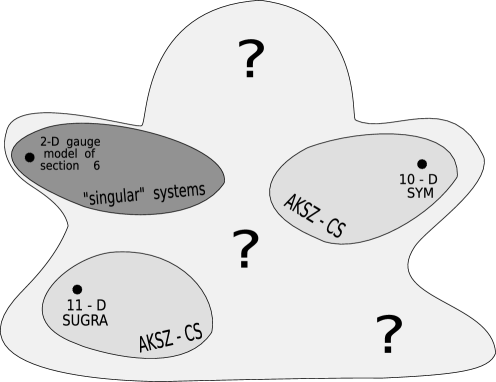
Figure 14: An illustration on the structure of the space of effective theories.

Different "singular" theories (black points) representing 10-D SYM, 11-D SUGRA, 2-D model of section 6 have different numbers $K$ of $\lambda_{\alpha}$ and $N$ - the number of quadrics. Hence they are from the different domains of the space of effective theories (see figure 14). The point is that in case $K\ \geq\ N$ there exist both "regular" and "singular" systems of quadrics. However if $N\ >\ K$ there are no "regular" systems. All quadrics are "singular" in this case. Hence the theories 10-D SYM ($K=16$, $N=10$) and 11-D SUGRA ($K=32$, $N=11$) are indeed surrounded by AKSZ-CS theories in their domains (strictly speaking the theories 10-D SYM and 11-D SUGRA are obtained from the effective action only after $Z_{2}$ reduction, which is similar to the one discussed in section 2). However the 2-D model of section 6 ($K\ =\ 4$, $N\ =\ 5$) is surrounded again by singular theories. This fact is indicated in the figure 14. Even in case $K\geq N$ there could be small deformations of quadrics which remain the system $f^{\mu}(\lambda)$ "singular". Hence, even in this case "singular" theories are not single dots but can have some modules. The signs "?" stand in the figure because we do not know whether it is possible or not to deform the construction continuously from the one domain to an another.

8 Appendix. Algebraic Meaning of the Berkovits Complex

ABSTRACT

Complete "mathematical" proof of the theorem from the section 4 is given. Using the Zig-Zag (Tick-Tack-Toe) technique it is demonstrated that cohomologies of the Berkovits complex are in one-to-one correspondence with the cohomologies of certain complex with zero differential. This allows at once to write down explicit expressions (4.1) for all representatives of $\mathcal{H}(Q,O)$.

In the main part of the paper we have studied the complex

$$C[\lambda,\theta]/I_{f}$$

with the differential

$$Q=\lambda^{\alpha}\frac{\partial}{\partial\theta^{\alpha}}$$

where $I_{f}$ is the ideal in $C[\lambda]$ generated by a set of quadrics $f_{\mu}(\lambda)$. We are interested in this complex because its cohomologies correspond to polarizations of fields in various (supersymmetric) quantum field theories.

At first glance this complex looks like another trick in supersymmetry. However (like many other tricks) this one is also related to some algebro-geometric construction. One can show that Berkovits complex is nothing but the complex computing the higher derived functor $Tor^{*}$ between two modules over the ring $C[\lambda]$.

Here we will give an elementary explanation of this fact. It would also explain why cohomologies of Berkovits complex are computed in terms of relations between relations.

First, let us explain what is the minimal free resolution. Consider the sequence:

$$\setcounter{MaxMatrixCols}{13}\begin{CD}.......\ @>{B}>{}>\ C^{M_{2}}[\lambda]\ @>{B}>{}>\ C^{M_{1}}[\lambda]\ @>{B}>{}>\ C^{N}[\lambda]\ @>{B}>{}>\ C[\lambda]\ @>{\widetilde{B}}>{}>\ S\ @>{0}>{}>\ 0\end{CD}$$ (51)

Here $C[\lambda]$ is a ring of polynomials, $C^{N}[\lambda]$, $C^{M_{1}}[\lambda]$, $C^{M_{2}}[\lambda]$ is respectively $N$, $M_{1}$ and $M_{2}$ copies of $C[\lambda]$, and $S$ is the coset $S=C[\lambda]/I_{f}$. The differential in this complex is defined as follows: the first differential from the right is simply zero, the second one - $\widetilde{B}$ makes factorization over the ideal $I_{f}$. To define other maps introduce a basis in the spaces $C^{N}[\lambda]$, $C^{M_{1}}[\lambda]$, $C^{M_{2}}[\lambda]$, … The basis elements are $e_{\mu}$ ($\mu=1..N$), $e_{A_{1}}$ ($A_{1}=1..M_{1}$), $e_{A_{2}}$ ($A_{2}=1..M_{2}$),… The action of $B$ is given by:

$$\begin{array}[]{c}B(e_{\mu})\ =\ f_{\mu}\\ B(e_{A_{1}})\ =\ G_{A_{1}}^{(1)\ \mu}\ e_{\mu}\\ B(e_{A_{2}})\ =\ G_{A_{2}}^{(2)\ A_{1}}\ e_{A_{1}}\\ ..............................................\end{array}$$ (52)

where $G_{A_{1}}^{(1)\ \mu}(\lambda)$ is the fundamental system of relations at the first level, $G_{A_{2}}^{(2)\ A_{1}}(\lambda)$ are the second-level fundamental relations and so on. This sequence is schematically depicted in the figure 15.

$$\setcounter{MaxMatrixCols}{11}\begin{CD}\!\!\!C^{M_{2}}[\lambda]\ @>{B}>{}>\ \ \ C^{M_{1}}[\lambda]\ \ @>{B}>{}>\ \ C^{N}[\lambda]\ \ \ @>{B}>{}>\ \ C[\lambda]\ \ \ @>{\widetilde{B}}>{}>\ \ \ \ \ S\ \ \ \ \ \ \ @>{0}>{}>\ \ \ \ \ \ \ 0\end{CD}$$

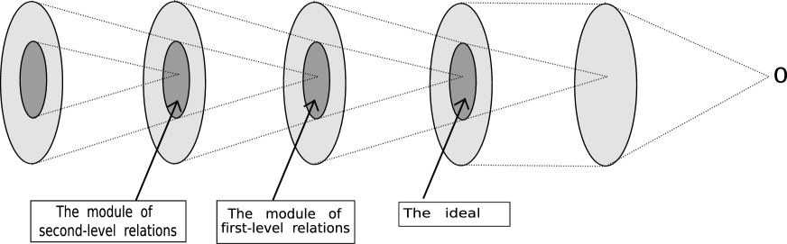
Figure 15: The free resolution.

In this figure light ovals denote the spaces $S$, $C[\lambda]$, $C^{N}[\lambda]$, $C^{M_{1}}[\lambda]$,… Each space contains a subspace (dark oval) which is mapped to zero by the differential. For example, operator $\widetilde{B}:\ C[\lambda]\ \longrightarrow\ S$ maps each element of the ideal $I_{f}$ (dark oval in $C[\lambda]$) to zero. At the previous step differential $B:\ C^{N}[\lambda]\ \longrightarrow\ C[\lambda]$ maps an arbitrary element $P^{\mu}(\lambda)e_{\mu}$ of $C^{N}[\lambda]$ onto $B(P^{\mu}(\lambda)e_{\mu})\ =\ P^{\mu}(\lambda)f_{\mu}(\lambda)$ - the element of the ideal. Hence, the pre-image of the ideal $I_{f}$ is the whole space $C^{N}[\lambda]$. This fact is illustrated in the figure 15 by the conic-like dashed lines. The free module $C^{N}[\lambda]$ again contains the subspace which is mapped to zero. This subspace is given by the elements $P^{\mu}(\lambda)e_{\mu}$, satisfying $B(P^{\mu}(\lambda)e_{\mu})\ =\ P^{\mu}(\lambda)f_{\mu}(\lambda)\ =\ 0$. Hence, the dark oval in $C^{N}[\lambda]$ is the module of first-level relations. Again, the pre-image of this module is the whole space $C^{M_{1}}[\lambda]$. Indeed, the arbitrary element $P^{A}(\lambda)e_{A}$ is mapped to $B(P^{A}(\lambda)e_{A})\ =\ P^{A}(\lambda)G_{A}^{(1)\ \mu}e_{\mu}$ which is a relation since $G_{A}^{(1)\ \mu}(\lambda)$ is a fundamental relation ( $G_{A}^{(1)\ \mu}f_{\mu}(\lambda)\ =\ 0$ ). Similar arguments can be applied to higher terms $C^{M_{2}}[\lambda]$,  $C^{M_{3}}[\lambda]$ and so on. From the figure 15 it is obvious that the sequence satisfies two properties:

1. Double action of the differential on an arbitrary element of the sequence gives zero (this is clear from the dashed lines in figure 15): $B^{2}\ =\ 0$.
   

2. This sequence has no cohomologies: each closed element is exact (again, this follows from the dashed lines).
   

The sequence, satisfying these two conditions is called the minimal free resolution. Minimality means that the elements of the fundamental system of relations are linearly independent. In this sequence most of terms are n-copies of the ring $C[\lambda]$. Hence, they are free modules. However, the first term $S$ is given by the coset, hence is far from being free.

Now we are ready to present the crucial instrument of the construction. Consider the bi-complex with differentials $B$ and $Q$ which can be written as the table:

$$\setcounter{MaxMatrixCols}{13}\begin{CD}.....@>{Q}>{}>\ [F(\lambda,\theta^{2})]\ @>{Q}>{}>\ [F(\lambda,\theta)]\ @>{Q}>{}>\ [F(\lambda)]\\ @A{}A{\widetilde{B}}A@A{}A{\widetilde{B}}A@A{}A{\widetilde{B}}A\\ .....@>{Q}>{}>\ F(\lambda,\theta^{2})\ @>{Q}>{}>\ F(\lambda,\theta)\ @>{Q}>{}>\ F(\lambda)\ @>{\widetilde{Q}}>{}>\ c\\ @A{}A{B}A@A{}A{B}A@A{}A{B}A@A{}A{0}A\\ .....@>{Q}>{}>\ F^{\mu}(\lambda,\theta^{2})e_{\mu}\ @>{Q}>{}>\ F^{\mu}(\lambda,\theta)e_{\mu}\ @>{Q}>{}>\ F^{\mu}(\lambda)e_{\mu}\ @>{\widetilde{Q}}>{}>\ c^{\mu}e_{\mu}\\ @A{}A{B}A@A{}A{B}A@A{}A{B}A@A{}A{0}A\\ .....@>{Q}>{}>\ F^{A_{1}}(\lambda,\theta^{2})e_{A_{1}}\ @>{Q}>{}>\ F^{A_{1}}(\lambda,\theta)e_{A_{1}}\ @>{Q}>{}>\ F^{A_{1}}(\lambda)e_{A_{1}}\ @>{\widetilde{Q}}>{}>\ c^{A}e_{A}\\ @A{}A{B}A@A{}A{B}A@A{}A{B}A@A{}A{0}A\\ @ ......@ ......@ ......@ ......\\ \end{CD}$$ (53)

\begin{picture}(10.0,10.0)(30.0,30.0) \put(0.0,0.0){} \put(0.0,0.0){} \end{picture}

The first line - the horizontal margin of the table - is the Berkovits complex. The differential is given by $Q=\lambda_{\alpha}\frac{\partial}{\partial\theta_{\alpha}}$ which acts in the space $O[\theta_{\alpha}\ \!,\ \!\lambda_{\alpha}\ |\ f^{\mu}(\lambda)]$. The grading in this space is given by the degree of $\theta$ and $Q$ decreases the grading. We use the notations $[F(\lambda)]$,  $[F(\lambda,\theta)]$,  $[F(\lambda,\theta^{2})]$,… to represent equivalence classes of functions, of certain degree in $\theta_{\alpha}$, in the space $O[\theta_{\alpha}\ \!,\ \!\lambda_{\alpha}\ |\ f^{\mu}(\lambda)]\ =\ C[\lambda,\theta]\diagup I_{f}$.

Each term of the Berkovits complex is resolved in vertical direction by the free resolution of figure 15. This means that one can think about each column in the table as the tensor product the free resolution by the functions of certain degree in $\theta_{\alpha}$. This resolution is equipped with the action of the differential $B$, defined in (52), and $\widetilde{B}$ which acts when one jumps from the table to the horizontal margin of the table (the sequence above the horizontal black line).

Thus we see that the table is equipped with the structure of the free resolution in the vertical direction. It happens that it is possible to build the complex on the vertical margin of the table (to the right of the black vertical line) in such a way that each horizontal sequence will be again a free resolution. To demonstrate this take as an example the second line of the table:

$$\setcounter{MaxMatrixCols}{11}\begin{CD}.....@>{Q}>{}>\ F^{\mu}(\lambda,\theta^{2})e_{\mu}\ @>{Q}>{}>\ F^{\mu}(\lambda,\theta)e_{\mu}\ @>{Q}>{}>\ F^{\mu}(\lambda)e_{\mu}\ @>{\widetilde{Q}}>{}>\ c^{\mu}e_{\mu}\ @>{0}>{}>\ 0\end{CD}$$ (54)

Since within the table (below the black horizontal line and to the left from the vertical one) there are no any constraints, like $f^{\mu}(\lambda)$ , the sequence (54) is free of cohomologies in the sector of $\theta$, $\theta^{2}$, $\theta^{3}$ and so on. This is true due to $Ker(Q)\ =\ 0$ in the ring $C[\lambda,\theta]$ in these sectors. Still, the question remains in the sector $F^{\mu}(\lambda)e_{\mu}$ of zero degree in $\theta$. To make the sequence exact, we define the $\widetilde{Q}$-operator (the jump from the table to the vertical margin) as factorization over the ideal $I_{\lambda}$, generated by the elements $\{\lambda_{1},\lambda_{2},...,\lambda_{K}\}$. In this case the image of $Q$-operator are functions $Q(F^{\mu}(\lambda,\theta)e_{\mu})$ at least linear in $\lambda_{\alpha}$ ( since $Q\ =\ \lambda_{\alpha}\frac{\partial}{\partial\theta_{\alpha}}$ ). Hence, operator $\widetilde{Q}$ (factorization over the ideal $I_{\lambda}$) maps such functions to zero, removing all cohomologies, in the sector $F^{\mu}(\lambda)e_{\mu}$. Thus to make the sequence (54) exact the complex on the vertical margin should be defined in the space $C[\lambda]\diagup I_{\lambda}\ =\ \mathbb{C}$ of complex numbers. Hence, the differential $B$, which is defined through relations (52) is simply zero on the vertical margin, due to the fact that fundamental relations $G^{(1)}(\lambda)$, $G^{(2)}(\lambda)$,… are at least linear in $\lambda_{\alpha}$. This fact is indicated on the vertical margin of (53) where the differential $B$ is reduced to $B\ =\ 0$ because of factorization over the ideal $I_{\lambda}$.

Concluding the presentation of the bi-complex, we summarize that it is written as the table (below the black horizontal line and to the left from the vertical one). This table has two margins: horizontal (above the horizontal line) and vertical (to the right of the vertical line). Horizontal margin is the Berkovits complex with operator $Q$, acting in the space $O[\theta_{\alpha}\ \!,\ \!\lambda_{\alpha}\ |\ f^{\mu}(\lambda)]$. Vertical margin is the complex with zero differential, acting in the spaces $C[\lambda]\diagup I_{\lambda}\ =\ c$, $\ C^{N}[\lambda]\diagup I_{\lambda}\ =\ c^{\mu}e_{\mu}$, $\ C^{M_{1}}[\lambda]\diagup I_{\lambda}\ =\ c^{A_{1}}e_{A_{1}}$ and so on. Here $c$, $c^{\mu}$, $c^{A_{1}}$, ….. are simply complex numbers. All the terms within the table are free of any factorization conditions.

Our last remark is that the action of operators $B$ and $Q$ is commutative $[B,\ Q]\ =\ 0$ on the table. This is true since the action of $B$ is defined through the fundamental system of relations (52), hence contains only multiplication by $\lambda$. Operator $Q$ also increases the number of $\lambda$. Since $\lambda_{\alpha}$ are commuting variables $[B,\ Q]\ =\ 0$. For the same reason commutators $[B,\ \widetilde{Q}]\ =\ 0$ and $[\widetilde{B},\ Q]\ =\ 0$ also vanish.

The Zig-Zag Theorem: the cohomologies of the Berkovits complex $\mathcal{H}(Q,O)$ are in one-to-one correspondence with the cohomologies of the complex at the vertical margin of the table.

The proof is in zig-zag jumps on the table (53). All arguments are similar for each term of the Berkovits complex. Thus we illustrate them taking the first non-trivial example - the class $[F(\lambda,\theta)]$. The zig-zag responsible for this term is presented in the table:

$$\setcounter{MaxMatrixCols}{13}\begin{CD}.....@>{Q}>{}>\ [F(\lambda,\theta^{2})]\ @>{Q}>{}>\ [F(\lambda,\theta)]\ @>{Q}>{}>\ [F(\lambda)]\\ @A{}A{\widetilde{B}}A@A{}A{\widetilde{B}}A@A{}A{\widetilde{B}}A\\ .....@>{Q}>{}>\ F(\lambda,\theta^{2})\ @>{Q}>{}>\ F(\lambda,\theta)\ @>{Q}>{}>\ F(\lambda)\ @>{\widetilde{Q}}>{}>\ c\\ @A{}A{B}A@A{}A{B}A@A{}A{B}A@A{}A{0}A\\ .....@>{Q}>{}>\ F^{\mu}(\lambda,\theta^{2})e_{\mu}\ @>{Q}>{}>\ F^{\mu}(\lambda,\theta)e_{\mu}\ @>{Q}>{}>\ F^{\mu}(\lambda)e_{\mu}\ @>{\widetilde{Q}}>{}>\ c^{\mu}e_{\mu}\\ @A{}A{B}A@A{}A{B}A@A{}A{B}A@A{}A{0}A\\ .....@>{Q}>{}>\ F^{A_{1}}(\lambda,\theta^{2})e_{A_{1}}\ @>{Q}>{}>\ F^{A_{1}}(\lambda,\theta)e_{A_{1}}\ @>{Q}>{}>\ F^{A_{1}}(\lambda)e_{A_{1}}\ @>{\widetilde{Q}}>{}>\ c^{A}e_{A}\\ @A{}A{B}A@A{}A{B}A@A{}A{B}A@A{}A{0}A\\ @ ......@ ......@ ......@ ......\\ \end{CD}$$ (55)

\begin{picture}(10.0,10.0)(30.0,30.0) \put(0.0,0.0){} \put(0.0,0.0){} \put(0.0,0.0){} \put(0.0,0.0){} \end{picture}

In the step1 of the proof we show that each $Q$-closed element in the space $[F(\lambda,\theta)]$ has a corresponding element in the sector $c^{\mu}e_{\mu}$ of the vertical complex. Since the complex has zero differential this element is $0$-closed. In the step2 we show that each $Q$-exact element in the sector $[F(\lambda,\theta)]$ is mapped to zero in the sector $c^{\mu}e_{\mu}$ (by the same zig-zag). Since the vertical complex has zero differential, it has no exact expressions. Hence, according to step1 and step2 we conclude that there is a map from the cohomologies of the Berkovits complex to the cohomologies of the vertical complex. The only question remains if this map is a one-to-one correspondence. To convince that it is the case, in step3 we start from the certain element in the sector $[F(\lambda,\theta)]$, then pass through the zig-zag to the vertical complex and then, along the same zig-zag, in the opposite direction. The fact that we obtain the same element completes the proof that the zig-zag map is the one-to-one correspondence.

step1     Suppose the class $[F(\lambda,\theta)]$ is $Q$-closed. This means that $QF(\lambda,\theta)\ =\ c^{\mu}(\lambda)f_{\mu}(\lambda)$, where $c^{\mu}(\lambda)$ are some coefficients. We are going to pass along the zig-zag, indicated in (55), to the vertical complex and find the corresponding element $c^{\mu}\ \!\!e_{\mu}$ in it. This element is $0$-closed. Since the vertical column

$$\begin{CD}.....@>{B}>{}>\ F^{\mu}(\lambda,\theta)e_{\mu}\ @>{B}>{}>\ F(\lambda,\theta)\ @>{\widetilde{B}}>{}>\ [F(\lambda,\theta)]\ @>{0}>{}>\ 0\end{CD}$$

is the free resolution of figure 15 and the last term $[F(\lambda,\theta)]$ in it is mapped to zero, one can apply operator $\widetilde{B}^{-1}$ to $[F(\lambda,\theta)]$, because the free resolution is free from cohomologies. Define the action of $\widetilde{B}^{-1}$ as

$$\widetilde{B}^{-1}\Big{(}[F(\lambda,\theta)]\Big{)}\ =\ F(\lambda,\theta)\$$

Now we have passed through the first step of the zig-zag and have jumped from the horizontal margin into the space $F(\lambda,\theta)$ of the table. Next step of the zig-zag is application of $Q$-operator. The result is:

$$Q\Big{(}\widetilde{B}^{-1}[F(\lambda,\theta)]\ \ +\ \ \widetilde{B}-\!\!\!\begin{array}[]{c}$closed$\end{array}\Big{)}$$ (56)

Applying $\widetilde{B}^{-1}$ we have a freedom to add $\widetilde{B}$-closed expression. Now we have jumped into the space $F(\lambda)$ on the table (55). Next step is application of $B^{-1}$. Since the vertical sequence is exact this is possible only if $\widetilde{B}Q\Big{(}\widetilde{B}^{-1}[F(\lambda,\theta)]\ +\ \ \widetilde{B}\!-\!\!\!\begin{array}[]{c}$closed$\end{array}\Big{)}\ =\ 0$. Simple computation gives:

$$\widetilde{B}Q\Big{(}\widetilde{B}^{-1}[F(\lambda,\theta)]\ +\ \ \widetilde{B}\!-\!\!\!\begin{array}[]{c}$closed$\end{array}\Big{)}\ =\ Q\widetilde{B}\Big{(}\widetilde{B}^{-1}[F(\lambda,\theta)]\ +\ \ \widetilde{B}\!-\!\!\!\begin{array}[]{c}$closed$\end{array}\Big{)}\ =\ Q\widetilde{B}\widetilde{B}^{-1}[F(\lambda,\theta)]\ =\ Q[F(\lambda,\theta)]\ =\ 0$$

In the first equality we used that $[Q,\ \widetilde{B}]\ =\ 0$, in the second one that $\widetilde{B}(\ \widetilde{B}\!-\!\!\!\begin{array}[]{c}$closed$\end{array})\ =\ 0$. In the last equality we explore that the class $[F(\lambda,\theta)]$ is $Q$-closed. Thus, it is possible to apply operator $B^{-1}$ to (56). Now we have come to the term $F^{\mu}(\lambda)e_{\mu}$ in the table (55). The last step of the zig-zag is to jump from the table to the vertical margin. This can be done by application of operator $\widetilde{Q}$. The result is:

$$\widetilde{Q}\bigg{(}B^{-1}\ Q\Big{(}\widetilde{B}^{-1}[F(\lambda,\theta)]\ +\ \widetilde{B}\!-\!\!\!\begin{array}[]{c}$closed$\end{array}\Big{)}\ +\ B\!-\!\!\!\begin{array}[]{c}$closed$\end{array}\bigg{)}$$

This expression is a representative of the class $c^{\mu}e_{\mu}$ of the complex on the vertical margin. Since the differential in this vertical complex is zero, this expression realizes the map from $Q$-closed classes $[F(\lambda,\theta)]$ to the $0$-closed elements of the vertical complex. It should be emphasized that this zig-zag can be done only in case $[F(\lambda,\theta)]$ is $Q$-closed.

Above we have done detailed calculation, emphasizing all ambiguities which can arise while inverting operator $B$. However it is clear, that since we used explicit basis for defining the action of $B$, it is possible to define $B^{-1}$ as

$$\begin{array}[]{c}B^{-1}(f_{\mu}(\lambda))\ =\ e_{\mu}\\ B^{-1}(G_{A}^{(1)\ \mu}e_{\mu})\ =\ e_{A}\\ ..........................................\end{array}$$ (57)

The same is true for the operator $Q^{-1}$. According to (32) anticommutator $\{D,\ Q\}\ =\ deg$, hence one can think that $Q^{-1}\ =\ \widetilde{D}\ =\ \frac{D}{deg}$. For the following we use these explicit expressions for the inverse operators, however this is not necessary for completing the proof.

step2    Suppose we start from exact class $[F(\lambda,\theta)]\ =\ Q[G(\lambda,\theta^{2})]$. This means that $[F(\lambda,\theta)]\ =\ QG(\lambda,\theta)\ +\ c^{\mu}(\lambda,\theta)f_{\mu}(\lambda)$. Application of $\widetilde{B}^{-1}$ to such class gives:

$$\widetilde{B}^{-1}[F(\lambda,\theta)]\ =\ QG(\lambda,\theta)\ +\ c^{\mu}(\lambda,\theta)f_{\mu}(\lambda)$$

with probably another coefficients $c^{\mu}(\lambda,\theta)$. Applying operator $Q$ to this expression one can get

$$Q\widetilde{B}^{-1}[F(\lambda,\theta)]\ =\ Q\big{(}c^{\mu}(\lambda,\theta)\big{)}\ f_{\mu}(\lambda)$$

Application of $\widetilde{B}$ to this result gives zero, since $Q(c^{\mu}(\lambda,\theta))\ f_{\mu}(\lambda)$ belongs to the ideal $I_{f}$. Hence, one can apply $B^{-1}$:

$$B^{-1}Q\widetilde{B}^{-1}[F(\lambda,\theta)]\ =\ Q\big{(}c^{\mu}(\lambda,\theta)\big{)}\ e_{\mu}$$ (58)

The last step is application of $\widetilde{Q}$ to this result. Since the function $c^{\mu}(\lambda,\theta)$ is linear in $\theta_{\alpha}$, expression $Qc^{\mu}(\lambda,\theta)$ is at least linear in $\lambda_{\alpha}$, because $Q\ =\ \lambda_{\alpha}\frac{\partial}{\partial\theta_{\alpha}}$. Hence the application of $\widetilde{Q}$ to (58) gives zero, since $\widetilde{Q}$ is factorization over the ideal $I_{\lambda}$. This completes the proof that all $Q$-exact classes on the horizontal margin of (55) are mapped to zero on the vertical margin.

step3    After fixation of all ambiguities in the inverting of operators $Q$ and $B$, step3 is almost obvious. Suppose $A$ is the element of cohomologies $\mathcal{H}(Q,\ O)$ in the sector $[F(\lambda,\theta)]$. Following the zig-zag, we come to the vertical margin by applying

$$\widetilde{Q}\ B^{-1}\ Q\ \widetilde{B}^{-1}\ A$$

Passing through the same zig-zag in the opposite direction one obtains

$$\widetilde{B}\ Q^{-1}\ B\ \widetilde{Q}^{-1}\ \widetilde{Q}\ B^{-1}\ Q\ \widetilde{B}^{-1}\ A\ \ =\ \ A$$

One should also take into account the possibility to pass from an arbitrary element $c^{\mu}e_{\mu}$ to the corresponding element in the sector $[F(\lambda,\theta)]$. The arguments are similar to that of step1 and step2. First one obtains $\widetilde{Q}^{-1}\big{(}c^{\mu}e_{\mu}\big{)}\ =\ c^{\mu}e_{\mu}$ - the element of $F^{\mu}(\lambda)e_{\mu}$. Then, applying operator $B$, we get the element $B\big{(}c^{\mu}e_{\mu}\big{)}\ =\ c^{\mu}f_{\mu}(\lambda)$ of $F(\lambda)$. Since $f^{\mu}(\lambda)$ are quadratic in $\lambda_{\alpha}$, action of operator $\widetilde{Q}(c^{\mu}f_{\mu})\ =\ 0$ vanishes. Hence, one can apply operator $Q^{-1}$, because the horizontal sequence is exact. After that we have jumped into the space $F(\lambda,\theta)$. Last step is application of operator $\widetilde{B}$.

The same construction can be straightforwardly realized for higher degrees in $\theta_{\alpha}$. Hence the proof of The Zig-Zag Theorem is finished.

Our last remark is that calculation of Berkovits cohomologies on the horizontal margin of the table is a difficult mathematical problem. However, calculation of cohomologies on the vertical margin is almost automatic. Since differential in this complex is zero, the whole space of complex coincides with its cohomologies. Hence, to calculate the cohomology of Berkovits complex one can take a space from the vertical complex, for example $c^{\mu}\ e_{\mu}$ (where $c^{\mu}$ are arbitrary numerical coefficients) and apply zig-zag to it.

$$\widetilde{B}\ Q^{-1}\ B\ \widetilde{Q}^{-1}(c^{\mu}\ e_{\mu})\ =\ \widetilde{B}\ Q^{-1}\ B\big{(}c^{\mu}\ e_{\mu}\big{)}\ =\ c^{\mu}\ \widetilde{B}\ Q^{-1}\ \big{(}f_{\mu}\big{)}\ =\ c^{\mu}\ \widetilde{B}\ \big{(}\widetilde{D}f_{\mu}\big{)}\ =\ c^{\mu}\widetilde{D}f_{\mu}$$ (59)

Here in the first equality we used that $\widetilde{Q}^{-1}$ is just a choice of representative and acts as identity on the basis elements. In the second equality we used (52). In the third equality the definition of $Q^{-1}$ was explored. The last equality is factorization over the ideal $I_{f}$. This technique allows to find explicit expression for the cohomology of Berkovits complex simply by the trivial application of the zig-zag to the obvious cohomology of the vertical complex.

This method can be straightforwardly generalized to the terms with higher degree in $\theta_{\alpha}$. For example, the zig-zag for the class $[F(\lambda,\theta^{2})]$ is given by:

$$\setcounter{MaxMatrixCols}{13}\begin{CD}.....@>{Q}>{}>\ [F(\lambda,\theta^{2})]\ @>{Q}>{}>\ [F(\lambda,\theta)]\ @>{Q}>{}>\ [F(\lambda)]\\ @A{}A{\widetilde{B}}A@A{}A{\widetilde{B}}A@A{}A{\widetilde{B}}A\\ .....@>{Q}>{}>\ F(\lambda,\theta^{2})\ @>{Q}>{}>\ F(\lambda,\theta)\ @>{Q}>{}>\ F(\lambda)\ @>{\widetilde{Q}}>{}>\ c\\ @A{}A{B}A@A{}A{B}A@A{}A{B}A@A{}A{0}A\\ .....@>{Q}>{}>\ F^{\mu}(\lambda,\theta^{2})e_{\mu}\ @>{Q}>{}>\ F^{\mu}(\lambda,\theta)e_{\mu}\ @>{Q}>{}>\ F^{\mu}(\lambda)e_{\mu}\ @>{\widetilde{Q}}>{}>\ c^{\mu}e_{\mu}\\ @A{}A{B}A@A{}A{B}A@A{}A{B}A@A{}A{0}A\\ .....@>{Q}>{}>\ F^{A_{1}}(\lambda,\theta^{2})e_{A_{1}}\ @>{Q}>{}>\ F^{A_{1}}(\lambda,\theta)e_{A_{1}}\ @>{Q}>{}>\ F^{A_{1}}(\lambda)e_{A_{1}}\ @>{\widetilde{Q}}>{}>\ c^{A}e_{A}\\ @A{}A{B}A@A{}A{B}A@A{}A{B}A@A{}A{0}A\\ @ ......@ ......@ ......@ ......\\ \end{CD}$$

\begin{picture}(10.0,10.0)(30.0,30.0) \put(0.0,0.0){} \put(0.0,0.0){} \put(0.0,0.0){} \put(0.0,0.0){} \put(0.0,0.0){} \put(0.0,0.0){} \end{picture}

Calculation similar to (59) gives:

$${\begin{split}\widetilde{B}\ Q^{-1}\ B\ Q^{-1}\ B\ \widetilde{Q}^{-1}\ \big{(}c^{A}e_{A}\big{)}\ =\ c^{A}\ \widetilde{B}\ Q^{-1}\ B\ Q^{-1}\ B\ \big{(}e_{A}\big{)}\ =\ c^{A}\ \widetilde{B}\ Q^{-1}\ B\ Q^{-1}\ \big{(}G_{A}^{(1)\ \mu}e_{\mu}\big{)}\ =\\ =\ c^{A}\ \widetilde{B}\ Q^{-1}\ B\ \widetilde{D}\big{(}G_{A}^{(1)\ \mu}\big{)}e_{\mu}\ =\ c^{A}\ \widetilde{B}\ Q^{-1}\ \widetilde{D}\big{(}G_{A}^{(1)\ \mu}\big{)}f_{\mu}\ =\ c^{A}\ \widetilde{B}\ \widetilde{D}\big{(}\widetilde{D}G_{A}^{(1)\ \mu}f_{\mu}\big{)}\ =\\ =\ c^{A}\ \widetilde{D}\big{(}\widetilde{D}G_{A}^{(1)\ \mu}f_{\mu}\big{)}\ \ \ \ \ \ \ \ \ \ \end{split}}$$

which is the third line of (4.1).

9 Acknowledgements

It is a pleasure to thank A. Morozov, M. Movshev, N. Nekrasov, V. Rubakov and A. Schwarz for useful discussions. Especially we would like to thank Alexei Gorodentsev for explaining the geometrical meaning of the discussed complex and the role of Zig-Zag technique. Also, we are indebted to V.Lysov for his contribution to our understanding of Feynman diagram technique in AKSZ-like theories and pointing out the mistake in the expressions (4.1) in the previous version of the paper. Also we are greatly indebted to A. Rosly for the careful reading of the manuscript and illuminating discussions. The work of A.L. was supported by the grants -8065.2006.2,  NWO-RFBR 047.011.2004.026 (RFBR 05-02-89000-NWOa)  and  INTAS 03-51-6346. The work of D.K. was supported by Dynasty Foundation and RFBR-08-02-00473.

References

- [1] E. Witten, ‘‘Noncommutative Geometry And String Field Theory,’’ Nucl. Phys. B 268 (1986) 253. E. Witten, ‘‘Interacting Field Theory Of Open Superstrings,’’ Nucl. Phys. B 276 (1986) 291. E. Witten, ‘‘Chern-Simons gauge theory as a string theory,’’ Prog. Math. 133, 637 (1995) [arXiv:hep-th/9207094].
- [2] N. Berkovits, ‘‘Covariant quantization of the superparticle using pure spinors,’’ JHEP 0109 (2001) 016 [arXiv:hep-th/0105050]. N. Berkovits, ‘‘ICTP lectures on covariant quantization of the superstring,’’ arXiv:hep-th/0209059.
- [3] M. Movshev and A. Schwarz, ‘‘On maximally supersymmetric Yang-Mills theories,’’ Nucl. Phys. B 681, 324 (2004) [arXiv:hep-th/0311132]. M. Movshev and A. Schwarz, ‘‘Algebraic structure of Yang-Mills theory,’’ arXiv:hep-th/0404183.
- [4] M. Movshev, ‘‘Yang-Mills theory and a superquadric,’’ arXiv:hep-th/0411111. M. Movshev, ‘‘Yang-Mills theories in dimensions 3,4,6,10 and Bar-duality,’’ arXiv:hep-th/0503165. M. Movshev, ‘‘On deformations of Yang-Mills algebras,’’ arXiv:hep-th/0509119. M. Movshev, ‘‘Deformation of maximally supersymmetric Yang-Mills theory in dimensions 10: An algebraic approach,’’ arXiv:hep-th/0601010.
- [5] A.Losev, V.Lysov, A.Gorodentsev "Dombay Seminars on Berkovits Theory", 2003, unpublished.
- [6] G. Barnich, M. Grigoriev, A. Semikhatov and I. Tipunin, ‘‘Parent field theory and unfolding in BRST first-quantized terms,’’ Commun. Math. Phys. 260 (2005) 147 [arXiv:hep-th/0406192]. G. Barnich and M. Grigoriev, ‘‘Parent form for higher spin fields on anti-de Sitter space,’’ arXiv:hep-th/0602166. M. Grigoriev, ‘‘Off-shell gauge fields from BRST quantization,’’ arXiv:hep-th/0605089.
- [7] N. Berkovits, ‘‘Super-Poincare covariant quantization of the superstring,’’ JHEP 0004 (2000) 018 [arXiv:hep-th/0001035].
- [8] E. Witten, ‘‘Twistor - Like Transform In Ten-Dimensions,’’ Nucl. Phys. B 266 (1986) 245. B. E. W. Nilsson, ‘‘Pure Spinors As Auxiliary Fields In The Ten-Dimensional Supersymmetric Yang-Mills Theory,’’ Class. Quant. Grav. 3 (1986) L41.
- [9] N. Berkovits and N. Nekrasov, ‘‘The character of pure spinors,’’ Lett. Math. Phys. 74 (2005) 75 [arXiv:hep-th/0503075].
- [10] I. A. Batalin and G. A. Vilkovisky, ‘‘Gauge Algebra And Quantization,’’ Phys. Lett. B 102 (1981) 27. I. A. Batalin and G. A. Vilkovisky, ‘‘Quantization Of Gauge Theories With Linearly Dependent Generators,’’ Phys. Rev. D 28 (1983) 2567 [Erratum-ibid. D 30 (1984) 508]. I. A. Batalin and E. S. Fradkin, ‘‘A Generalized Canonical Formalism And Quantization Of Reducible Gauge Theories,’’ Phys. Lett. B 122 (1983) 157. B. L. Voronov and I. V. Tyutin, ‘‘Formulation Of Gauge Theories Of General Form. I,’’ Theor. Math. Phys. 50 (1982) 218 [Teor. Mat. Fiz. 50 (1982) 333].
- [11] A. Schwarz, ‘‘Geometry of Batalin-Vilkovisky quantization,’’ Commun. Math. Phys. 155 (1993) 249 [arXiv:hep-th/9205088]. A. Schwarz, ‘‘Semiclassical approximation in Batalin-Vilkovisky formalism,’’ Commun. Math. Phys. 158 (1993) 373 [arXiv:hep-th/9210115].
- [12] M. Alexandrov, M. Kontsevich, A. Schwartz and O. Zaboronsky, ‘‘The Geometry of the master equation and topological quantum field theory,’’ Int. J. Mod. Phys. A 12 (1997) 1405 [arXiv:hep-th/9502010].
- [13] C. Becchi, A. Rouet and R. Stora, ‘‘Renormalization Of Gauge Theories,’’ Annals Phys. 98 (1976) 287;Commun. Math. Phys. 42 (1975) 127. I. V. Tyutin, ‘‘Gauge Invariance In Field Theory And Statistical Physics In Operator Formalism,’’ LEBEDEV-75-39
- [14] N. Berkovits, ‘‘Covariant quantization of the supermembrane,’’ JHEP 0209 (2002) 051 [arXiv:hep-th/0201151]. N. Berkovits and P. S. Howe, ‘‘Ten-dimensional supergravity constraints from the pure spinor formalism for the superstring,’’ Nucl. Phys. B 635 (2002) 75 [arXiv:hep-th/0112160]. M. Cederwall, B. E. W. Nilsson and D. Tsimpis, ‘‘Spinorial cohomology and maximally supersymmetric theories,’’ JHEP 0202 (2002) 009 [arXiv:hep-th/0110069].
- [15] L. Anguelova, P. A. Grassi and P. Vanhove, ‘‘Covariant one-loop amplitudes in D = 11,’’ Nucl. Phys. B 702 (2004) 269 [arXiv:hep-th/0408171]. P. A. Grassi and P. Vanhove, ‘‘Topological M theory from pure spinor formalism,’’ Adv. Theor. Math. Phys. 9 (2005) 285 [arXiv:hep-th/0411167].
- [16] I. Oda and M. Tonin, ‘‘Worldline approach of topological BF theory,’’ Phys. Lett. B 623 (2005) 155 [arXiv:hep-th/0506054].
- [17] N. Berkovits and O. Chandia, ‘‘Lorentz invariance of the pure spinor BRST cohomology for the superstring,’’ Phys. Lett. B 514 (2001) 394 [arXiv:hep-th/0105149]. N. Berkovits and S. A. Cherkis, ‘‘Pure spinors are higher-dimensional twistors,’’ JHEP 0412 (2004) 049 [arXiv:hep-th/0409243]. N. Berkovits and O. Chandia, ‘‘Massive superstring vertex operator in D = 10 superspace,’’ JHEP 0208 (2002) 040 [arXiv:hep-th/0204121]. I. Oda and M. Tonin, ‘‘On the b-antighost in the pure spinor quantization of superstrings,’’ Phys. Lett. B 606 (2005) 218 [arXiv:hep-th/0409052]. M. Matone, L. Mazzucato, I. Oda, D. Sorokin and M. Tonin, ‘‘The superembedding origin of the Berkovits pure spinor covariant quantization of superstrings,’’ Nucl. Phys. B 639 (2002) 182 [arXiv:hep-th/0206104]. C. R. Mafra, ‘‘Four-point one-loop amplitude computation in the pure spinor formalism,’’ JHEP 0601 (2006) 075 [arXiv:hep-th/0512052]. B. C. Vallilo, ‘‘Flat currents in the classical AdS(5) x S**5 pure spinor superstring,’’ JHEP 0403 (2004) 037 [arXiv:hep-th/0307018]. I. Oda and M. Tonin, ‘‘On the Berkovits covariant quantization of GS superstring,’’ Phys. Lett. B 520 (2001) 398 [arXiv:hep-th/0109051]. Y. Aisaka and Y. Kazama, ‘‘A new first class algebra, homological perturbation and extension of pure spinor formalism for superstring,’’ JHEP 0302 (2003) 017 [arXiv:hep-th/0212316]. Y. Aisaka and Y. Kazama, ‘‘Origin of pure spinor superstring,’’ JHEP 0505 (2005) 046 [arXiv:hep-th/0502208]. P. A. Grassi, G. Policastro, M. Porrati and P. Van Nieuwenhuizen, ‘‘Covariant quantization of superstrings without pure spinor constraints,’’ JHEP 0210 (2002) 054 [arXiv:hep-th/0112162].
- [18] V. Alexandrov, D. Krotov, A. Losev and V. Lysov, ‘‘On Pure Spinor Superfield Formalism,’’ JHEP 0710 (2007) 074 [arXiv:0705.2191 [hep-th]].