Wilson’s Renormalization Group
and Its Applications in Perturbation Theory

Abstract

The general prescription for constructing the continuum limit of a field theory is explained using Wilson’s renormalization group. We then formulate the renormalization group in perturbation theory and apply it to $4$ dimensional $\phi^{4}$ and QED.

0 Introduction

Quantum Field Theory has a very long history. It started with the quantization of the electromagnetic field by Dirac in 1927.[1] This is almost 80 years ago. Currently every student of particle theory (and string theory) takes a course on quantum field theory which covers such important topics as perturbative renormalization, gauge theories, spontaneous symmetry breaking, and the Higgs mechanism. I assume that you know at least perturbative renormalization.

The problem with perturbative renormalization theory is the lack of physical insights. It consists of procedures for subtracting UV divergences to get finite results. Unfortunately, many if not most people still regard renormalization this way. It is the purpose of the next four lectures to introduce the physics of renormalization.

The essence of modern renormalization theory has been known for a long time. It was initiated mainly by Ken Wilson in the late 60’s. You must have heard the expressions such as renormalization group (RG), RG flows, fixed points, relevant and irrelevant parameters. Unfortunately there is no textbook introducing these ideas of Wilson’s. After 40 years, the best reference is still the two lecture notes [2, 3] by himself. I believe Wilson’s renormalization theory is best studied in a second course on field theory, and my four lectures will give merely an outline.

The four lectures are organized as follows. In lecture 1, we start with concrete examples of renormalization to introduce the relation between criticality and renormalizability. We will give hardly any derivation, but the examples will illuminate the meaning of renormalization. In lecture 2, we introduce the exact renormalization group (ERG) as a tool to understand the nature of renormalization. The emphasis is on the ideas of fixed points, relevance/irrelevance of parameters, and universality. In lectures 3 & 4, we apply Wilson’s exact renormalization group to perturbation theory. This was initiated by J. Polchinski in 1984.[4] We mainly discuss the $\phi^{4}$ theory in $4$ dimensions in lecture 3, and QED in lecture 4. I think that it is a reflection of the depth of the renormalization group that after almost 40 years of conception it is still under active research.[5]

1 Lecture 1 – Continuum Limits

The purpose of the first lecture is to familiarize ourselves with the concept of renormalization through concrete examples. Before we start, we should agree on the use of the euclidean metric as opposed to the Minkowski metric.

$$\eta_{\mu\nu}=\mathrm{diag}(1,-1,-1,-1)\longrightarrow\delta_{\mu\nu}=\mathrm{diag}(1,1,1,1)$$

Given an $n$-point Green function of a scalar field $\phi$

$$\left\langle\phi(\vec{x}_{1},x_{1}^{0})\cdots\phi(\vec{x}_{n},x_{n}^{0})\right\rangle$$

we obtain an $n$-point correlation function

$$\left\langle\phi(x_{1})\cdots\phi(x_{n})\right\rangle$$

by the analytic continuation

$$x_{i}^{0}\longrightarrow-ix_{i}^{4}\qquad(i=1,\cdots,n)$$

For example, the free scalar propagator

$$\int\frac{d^{D}p}{(2\pi)^{D}}\frac{i~{}\mathrm{e}^{-ipx}}{p^{2}-m^{2}+i\epsilon}\qquad(px\equiv p^{0}x^{0}-\vec{p}\cdot\vec{x})$$

becomes

$$\int\frac{d^{D}p}{(2\pi)^{D}}\frac{\mathrm{e}^{ipx}}{p^{2}+m^{2}}\qquad(px\equiv p_{4}x_{4}+\vec{p}\cdot\vec{x})$$

Problem 1-1: Derive this.
Hence, the free propagator in Minkowski space

$$\frac{i}{p^{2}-m^{2}+i\epsilon}$$

becomes

$$\frac{1}{p^{2}+m^{2}}$$

in euclidean space.

1.1 The idea of a continuum limit

The idea of a continuum limit is very simple and must be already familiar to you. We consider a theory with a momentum cutoff $\Lambda$, meaning that the theory is defined only up to the scale $\Lambda$. For example, a lattice theory defined on a cubic lattice of a lattice unit

$$a=\frac{1}{\Lambda}$$

has the momentum cutoff $\Lambda$. (Figure 1)

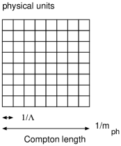
Figure 1: A cubic lattice in physical units

The continuum limit is the limit

$$\Lambda\to\infty$$

and renormalization is the specific way of taking the continuum limit so that the physical mass scale $m_{\mathrm{ph}}$, say the mass of an elementary particle, remains finite.

From the viewpoint of a lattice theory, it is more natural to measure distances in lattice units. Hence, the lattice unit becomes simply $1$.

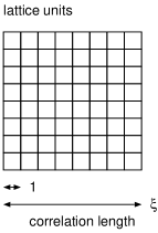
Figure 2: A cubic lattice in lattice units

In this convention, the Compton length or equivalently the inverse of the physical mass is a dimensionless number $\xi$ called the correlation length. Therefore, we obtain

$$\xi\,a=\frac{1}{m_{\mathrm{ph}}}\Longrightarrow\framebox{$\displaystyle\xi=\frac{\Lambda}{m_{\mathrm{ph}}}$}$$

Clearly, $\xi\to\infty$ as we take $\Lambda\to\infty$ while keeping $m_{\mathrm{ph}}$ finite. Thus, as we take the continuum limit, the lattice theory must obtain an infinite correlation length.

A lattice theory with an infinite correlation length is called a critical theory. Therefore, to obtain a continuum limit the corresponding lattice theory must be critical. Let us look at examples.

1.2 Ising model in $2$ dimensions

The Ising model on a square lattice is defined by the action

$$S=-K\sum_{\vec{n}=(n_{1},n_{2})}\sum_{i=1}^{2}\sigma_{\vec{n}}\sigma_{\vec{n}+\hat{i}}$$

At each site $\vec{n}$ of the lattice, we introduce a classical spin variable $\sigma_{\vec{n}}=\pm 1$. The parameter $K$ is a dimensionless positive constant, which we can regard as the inverse of a reduced (i.e., dimensionless) temperature.

$$K\sim\frac{1}{T}$$

The partition function is defined by

$$Z(K)=\sum_{\sigma_{\vec{n}}=\pm 1}\mathrm{e}^{-S}$$

and the correlation functions are defined by

$$\left\langle\sigma_{\vec{n}_{1}}\cdots\sigma_{\vec{n}_{N}}\right\rangle_{K}=\frac{\sum_{\sigma=\pm 1}\sigma_{\vec{n}_{1}}\cdots\sigma_{\vec{n}_{N}}\mathrm{e}^{-S}}{Z(K)}$$

The action is invariant under the global $\mathbf{Z_{2}}$ transformation

$$(\forall\vec{n})\quad\sigma_{\vec{n}}\longrightarrow-\sigma_{\vec{n}}$$

With respect to this symmetry, the model has two phases:

• High temperature phase $K<K_{c}$: the $\mathbf{Z}_{2}$ symmetry is exact, and

  $$\left\langle\sigma_{\vec{n}}\right\rangle=0$$

• Low temperature phase $K>K_{c}$: the $\mathbf{Z}_{2}$ symmetry is spontaneously broken, and

  $$\left\langle\sigma_{\vec{n}}\right\rangle=s(K)\neq 0$$

For large $|\vec{n}|$, the two-point function behaves exponentially as

$$\left\langle\sigma_{\vec{n}}\sigma_{\vec{0}}\right\rangle_{K}\sim\mathrm{e}^{-\frac{|\vec{n}|}{\xi}}$$

This defines the correlation length $\xi(K)$. At $K=K_{c}$ the theory is critical with $\xi=\infty$. Two critical exponents

$$\framebox{$\displaystyle y_{E}=1$}\quad\textrm{and}\quad\framebox{$\displaystyle x_{h}=\frac{1}{8}$}$$

characterize the theory near criticality as follows:

• As $K\to K_{c}$, the correlation length behaves as

  $$\xi\sim|K-K_{c}|^{-\frac{1}{y_{E}}}=\frac{1}{|K-K_{c}|}$$

• As $K\to K_{c}+0$, the VEV behaves as

  $$s\sim|K-K_{c}|^{\frac{h}{y_{E}}}=|K-K_{c}|^{\frac{1}{8}}$$

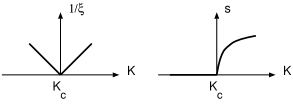
Figure 3: The critical exponents $y_{E},x_{h}$ characterize the correlation length $\xi$ and VEV $s$ near the critical point $K=K_{c}$.

The correlation functions near the critical point $K\simeq K_{c}$ obeys the scaling law:

$$\framebox{$\displaystyle\left\langle\sigma_{\vec{n}_{1}}\cdots\sigma_{\vec{n}_{N}}\right\rangle_{K}\simeq|K-K_{c}|^{N\frac{x_{h}}{y_{E}}}F_{N}^{\pm}\left(\frac{\vec{n}_{1}-\vec{n}_{N}}{\xi},\cdots,\frac{\vec{n}_{N-1}-\vec{n}_{N}}{\xi}\right)$}$$

where $\pm$ for $K>(<)K_{c}$. For $N>1$, the scaling law is valid only for large separation of lattice sites:

$$|\vec{n}_{i}-\vec{n}_{j}|\gg 1\quad(i\neq j)$$

For $N=1$, the scaling law simply boils down to the exponential behavior of $s(K)$ near criticality. For $N=2$, the scaling law gives

$$\left\langle\sigma_{\vec{n}}\sigma_{\vec{0}}\right\rangle_{K}\simeq|K-K_{c}|^{\frac{1}{4}}F_{2}^{\pm}\left(\frac{\vec{n}}{\xi}\right)$$

where $\xi\sim\frac{1}{|K-K_{c}|}$. For the limit to exist as $K\to K_{c}$, the function $F_{2}^{\pm}$ must behave like

$$F_{2}^{\pm}(x)\sim x^{-1/4}$$

for $x\ll 1$. Hence, at the critical point $K=K_{c}$, the two-point function is given by the exponential

$$\left\langle\sigma_{\vec{n}}\sigma_{\vec{0}}\right\rangle_{K_{c}}\sim\frac{1}{|\vec{n}|^{2x_{h}}}=\frac{1}{|\vec{n}|^{\frac{1}{4}}}\quad(|\vec{n}|\gg 1)$$

In fact this is another way of introducing the critical exponent $x_{h}$.

The scaling law introduced above implies that we can renormalize the Ising model to construct a scalar field theory as follows:

$$\framebox{$\displaystyle\left\langle\phi(\vec{r}_{1})\cdots\phi(\vec{r}_{N})\right\rangle_{m;\mu}\equiv\lim_{t\to\infty}\mathrm{e}^{\frac{Nt}{8}}\left\langle\sigma_{\vec{n}_{1}=\mu\vec{r}_{1}\mathrm{e}^{t}}\cdots\sigma_{\vec{n}_{N}=\mu\vec{r}_{N}\mathrm{e}^{t}}\right\rangle_{K=K_{c}-\frac{m}{\mu}\mathrm{e}^{-t}}$}$$

where both $m$ and $\mu$ have mass dimension $1$.

Let us explain this formula in several steps:

1. $K=K_{c}-\frac{m}{\mu}\mathrm{e}^{-t}$ — Hence, as $t\to\infty$, the theory approaches criticality. The particular $t$ dependence was chosen so that $\xi\propto\mathrm{e}^{t}$.

2. Necessity of $\mu$ — $\mu$ was introduced so that the physical length of a lattice unit is $\frac{1}{\mu}\mathrm{e}^{-t}$. Hence, $\vec{r}=\vec{n}\frac{1}{\mu}\mathrm{e}^{-t}$ has mass dimension $-1$, and $m$ has mass dimension $1$.

3. Given an arbitrary coordinate $\vec{r}$, $\vec{n}=\mu\vec{r}\mathrm{e}^{t}$ is not necessarily a vector with integer components. Since $\mathrm{e}^{t}\gg 1$, however, we can always find an integral vector $\vec{n}$ which approximates $\mu\vec{r}\mathrm{e}^{t}$ to the accuracy $\mathrm{e}^{-t}\ll 1$.

4. Applying the scaling law, we can compute the limit as

   $$\left\langle\phi(\vec{r}_{1})\cdots\phi(\vec{r}_{N})\right\rangle_{m;\mu}$$

   $$= \lim_{t\to\infty}\mathrm{e}^{\frac{Nt}{8}}|K-K_{c}|^{\frac{N}{8}}F_{N}^{\pm}\left(\frac{\mu\mathrm{e}^{t}|K-K_{c}|}{c_{\pm}}(\vec{r}_{1}-\vec{r}_{N}),\cdots\right)$$

   $$= \left(\frac{m}{\mu}\right)^{\frac{N}{8}}F_{N}^{\pm}\left(\frac{m}{c_{\pm}}(\vec{r}_{1}-\vec{r}_{N}),\cdots\right)$$

   where we used

   $$\xi\simeq\frac{c_{\pm}}{|K-K_{c}|}$$

   Thus, the limit exists. The limit depends not only on the mass parameter $m$ but also on the arbitrary mass scale $\mu$.

5. RG equation — The correlation function satisfies

   $$\left\langle\phi(\mathrm{e}^{-\Delta t}\vec{r}_{1})\cdots\phi(\mathrm{e}^{-\Delta t}\vec{r}_{N})\right\rangle_{m\mathrm{e}^{t};\mu}=\mathrm{e}^{N\frac{\Delta t}{8}}\left\langle\phi(\vec{r}_{1})\cdots\phi(\vec{r}_{N})\right\rangle_{m;\mu}$$

   This implies that the scale change of the coordinates

   $$(\forall i)\quad\vec{r}_{i}\longrightarrow\vec{r}_{i}\mathrm{e}^{-\Delta t}$$

   can be compensated by the change of the mass parameter $m$:

   $$m\longrightarrow m\mathrm{e}^{\Delta t}$$

   and renormalization of the field:

   $$\phi\longrightarrow\mathrm{e}^{\frac{\Delta t}{8}}\phi$$

   Hence, $y_{E}=1$ is the scale dimension of $m$, and $x_{h}=\frac{1}{8}$ is that of $\phi$. The general solution of the RG equation is given by the scaling formula with $F_{N}^{\pm}$ as arbitrary functions.

6. $\mu$ dependence (alternative RG equation)

   $$\left\langle\phi(\vec{r}_{1})\cdots\phi(\vec{r}_{N})\right\rangle_{m;\mu\mathrm{e}^{-\Delta t}}=\mathrm{e}^{\frac{\Delta t}{8}}\left\langle\phi(\vec{r}_{1})\cdots\phi(\vec{r}_{N})\right\rangle_{m;\mu}$$

   This is obtained from the previous RG equation by dimensional analysis. The change of $\mu$ is compensated by renormalization of $\phi$.

7. Elimination of $\mu$ — If we want, we can eliminate the arbitrary scale $\mu$ from the continuum limit by giving the mass dimension $\frac{1}{8}$ to the scalar field. By writing $\mu^{\frac{1}{8}}\phi$ as the new scalar field $\phi$, we obtain

   $$\left\langle\phi(\vec{r}_{1})\cdots\phi(\vec{r}_{N})\right\rangle_{m}=m^{\frac{N}{8}}F_{N}^{\pm}\left(\frac{m}{c_{\pm}}(\vec{r}_{1}-\vec{r}_{N}),\cdots\right)$$

Before ending, let us examine the short distance behavior using RG. The RG equation can be rewritten as

$$\left\langle\phi(\mathrm{e}^{-t}\vec{r}_{1})\cdots\phi(\mathrm{e}^{-t}\vec{r}_{N})\right\rangle_{m;\mu}=\mathrm{e}^{N\frac{t}{8}}\left\langle\phi(\vec{r}_{1})\cdots\phi(\vec{r}_{N})\right\rangle_{m\mathrm{e}^{-t};\mu}$$

Hence, in the short distance limit, the correlation functions are given by those at the critical point $m=0$:

$$\left\langle\phi(\mathrm{e}^{-t}\vec{r}_{1})\cdots\phi(\mathrm{e}^{-t}\vec{r}_{N})\right\rangle_{m;\mu}\stackrel{{\scriptstyle t\gg 1}}{{\simeq}}\mathrm{e}^{N\frac{t}{8}}\left\langle\phi(\vec{r}_{1})\cdots\phi(\vec{r}_{N})\right\rangle_{0;\mu}$$

Especially for the two-point function, we obtain

$$\left\langle\phi(\mathrm{e}^{-t}\vec{r})\phi(\vec{0})\right\rangle_{m;\mu}\stackrel{{\scriptstyle t\gg 1}}{{\simeq}}\frac{\mathrm{const}}{(\mu r\mathrm{e}^{-t})^{\frac{1}{4}}}$$

1.3 Ising model in $3$ dimensions

We can construct the continuum limit of the $3$ dimensional Ising model the same way as for the $2$ dimensional one. The only difference is the value of the critical exponents $y_{E}$ and $x_{h}$.

$$y_{E}\simeq 1.6,\quad\eta\equiv 2x_{h}-1\simeq 0.04$$

These are known only approximately. $\eta$ gives the difference of the scale dimension of the scalar field from the free field value, and is called the anomalous dimension.

In defining the continuum limit, we can give any engineering dimension to the scalar field. Here, let us pick $\frac{1}{2}$, the same as the free scalar field. The two-point function can be defined as

$$\left\langle\phi(\vec{r})\phi(\vec{0})\right\rangle_{g;\mu}\equiv\mu\lim_{t\to\infty}\mathrm{e}^{(1+\eta)t}\left\langle\sigma_{\vec{n}=\mu\vec{r}\mathrm{e}^{t}}\sigma_{\vec{0}}\right\rangle_{K=K_{c}-\frac{g}{\mu^{2}}\mathrm{e}^{-y_{E}t}}$$

Problem 1-2: Define the $n$-point function.
We have arbitrarily given the engineering $2$ to the parameter $g$.

The two-point function obeys the following RG equation:

$$\left\langle\phi(\vec{r}\mathrm{e}^{-\Delta t})\phi(\vec{0})\right\rangle_{g\mathrm{e}^{y_{E}\Delta t};\mu}=\mathrm{e}^{(1+\eta)\Delta t}\left\langle\phi(\vec{r})\phi(\vec{0})\right\rangle_{g;\mu}$$

This implies the short-distance behavior

$$\left\langle\phi(\vec{r}\mathrm{e}^{-t})\phi(\vec{0})\right\rangle_{g;\mu}\stackrel{{\scriptstyle t\gg 1}}{{\simeq}}\mathrm{const}\frac{\mu}{(\mu r\mathrm{e}^{-t})^{1+\eta}}$$

1.4 Alternative: $\phi^{4}$ on a cubic lattice

The same continuum limit can be obtained from a different model. Let $\phi_{\vec{n}}$ be a real variable taking a value from $-\infty$ to $\infty$. We consider the $\phi^{4}$ theory on a cubic lattice:

$$S=\sum_{\vec{n}}\left[\frac{1}{2}\sum_{i=1}^{3}\left(\phi_{\vec{n}+\hat{i}}-\phi_{\vec{n}}\right)^{2}+\frac{m_{0}^{2}}{2}\phi_{\vec{n}}^{2}+\frac{\lambda_{0}}{4!}\phi_{\vec{n}}^{4}\right]$$

where $\lambda_{0}>0$, but $m_{0}^{2}$ can be negative.

For $\lambda_{0}$ fixed, the theory has two phases depending on the value of $m_{0}^{2}$:

• symmetric phase $m_{0}^{2}>m_{0,cr}^{2}(\lambda_{0})$: $\mathbf{Z}_{2}$ is intact.

• broken phase $m_{0}^{2}<m_{0,cr}^{2}(\lambda_{0})$: $\mathbf{Z}_{2}$ is spontaneously broken, and $\left\langle\phi_{\vec{n}}\right\rangle\neq 0$.

Note that the critical value $m_{0,cr}^{2}(\lambda_{0})$ depends on $\lambda_{0}$.

The continuum limit is obtained as

$$\left\langle\phi(\vec{r})\phi(\vec{0})\right\rangle_{g;\mu}\equiv\mu\lim_{t\to\infty}\mathrm{e}^{(1+\eta)t}\left\langle\phi_{\vec{n}=\mu\vec{r}\mathrm{e}^{t}}\phi_{\vec{0}}\right\rangle_{m_{0}^{2}=m_{0,cr}^{2}(\lambda_{0})+\mathrm{e}^{-y_{E}t}\frac{g}{\mu^{2}}}$$

where $y_{E},\eta$ are the same critical exponents as in the Ising model. This limit is not necessarily independent of $\lambda_{0}$. For independence, we need to do rescale both $\phi$ and $g$:

$$\left\{\begin{array}[]{c@{~\longrightarrow~}c}\phi\hfil~{}\longrightarrow~{}&\sqrt{z(\lambda_{0})}~{}\phi\\ g\hfil~{}\longrightarrow~{}&z_{m}(\lambda_{0})~{}g\end{array}\right.$$

and define

$$\left\langle\phi(\vec{r})\phi(\vec{0})\right\rangle_{g;\mu}\equiv z(\lambda_{0})\mu\lim_{t\to\infty}\mathrm{e}^{(1+\eta)t}\left\langle\phi_{\vec{n}=\mu\vec{r}\mathrm{e}^{t}}\phi_{\vec{0}}\right\rangle_{m_{0}^{2}=m_{0,cr}^{2}(\lambda_{0})+\mathrm{e}^{-y_{E}t}z_{m}(\lambda_{0})\frac{g}{\mu^{2}}}$$

Universality consists of two statements:

1. $y_{E},\eta$ are the same as in the Ising model.

2. The continuum limit is the same as in the Ising model. (We only have to choose $z(\lambda_{0})$ and $z_{m}(\lambda_{0})$ appropriately.)

We have defined the continuum limit using the lattice units for the lattice theory. How do we take the continuum limit if we use the physical units instead? To go to the physical units, we assign the length

$$a=\frac{1}{\Lambda}=\frac{1}{\mu e^{t}}$$

to the lattice unit. The action is now given by

$$S=\underbrace{a^{3}\sum_{\vec{n}}}_{=\int d^{3}r}\Bigg{[}\frac{1}{2}\sum_{i=1}^{3}\underbrace{\frac{1}{a^{2}}\left(\varphi_{\vec{r}+a\hat{i}}-\varphi_{\vec{r}}\right)^{2}}_{=(\partial_{i}\varphi)^{2}}+\frac{m_{bare}^{2}}{2}\varphi_{\vec{r}}^{2}+\frac{\lambda_{bare}}{4!}\varphi_{\vec{r}}^{4}\Bigg{]}$$

where

$$\left\{\begin{array}[]{c@{~\equiv~}l}\vec{r}\hfil~{}\equiv~{}&\vec{n}a=\frac{\vec{n}}{\Lambda}\\ \varphi_{\vec{r}}\hfil~{}\equiv~{}&\frac{1}{\sqrt{a}}\phi_{\vec{n}}=\sqrt{\Lambda}\phi_{\vec{n}}\\ m_{bare}^{2}\hfil~{}\equiv~{}&\frac{m_{0}^{2}}{a^{2}}=m_{0}^{2}\Lambda^{2}\\ \lambda_{bare}\hfil~{}\equiv~{}&\frac{\lambda_{0}}{a}=\lambda_{0}\Lambda\end{array}\right.$$

Then, to obtain the continuum limit we must choose

$$\left\{\begin{array}[]{c@{~=~}l}m_{bare}^{2}\hfil~{}=~{}&\Lambda^{2}m_{0,cr}^{2}(\lambda_{0})+z_{m}(\lambda_{0})g\left(\frac{\Lambda}{\mu}\right)^{2-y_{E}}\\ \lambda_{bare}\hfil~{}=~{}&\Lambda\lambda_{0}\end{array}\right.$$

and we obtain

$$\left\langle\phi(\vec{r})\phi(\vec{0})\right\rangle_{g;\mu}=z(\lambda_{0})\lim_{\Lambda\to\infty}\left(\frac{\Lambda}{\mu}\right)^{\eta}\left\langle\varphi_{\vec{r}}\varphi_{\vec{0}}\right\rangle_{m_{bare}^{2},\lambda_{bare}}$$

Note that $\lambda_{0}>0$ is a finite arbitrary constant. The bare squared mass has not only a quadratic divergence but also a divergence of power $2-y_{E}\simeq 0.4$. The bare coupling is linearly divergent. We see clearly that the UV divergences of parameters are due to the use of physical units. If we use the lattice units, there is no divergence.

1.5 Ising model in $4$ dimensions

The $4$ dimensional case is very different from the lower dimensional cases in that we cannot take the continuum limit $\Lambda\to\infty$ without obtaining a free theory. This is called triviality. For example, we obtain

$$\left\langle\phi(\vec{r})\phi(\vec{0})\right\rangle_{m^{2};\mu} \equiv z\mu^{2}\lim_{t\to\infty}\mathrm{e}^{2t}\left\langle\sigma_{\vec{n}=\mu\vec{r}\mathrm{e}^{t}}\sigma_{\vec{0}}\right\rangle_{K=K_{c}-z_{m}\frac{m^{2}}{\mu^{2}}\mathrm{e}^{-2t}t^{-\beta_{m}}}$$

$$= \int_{p}\frac{\mathrm{e}^{ipr}}{p^{2}+m^{2}}$$

where

$$\beta_{m}=-\frac{1}{3}$$

and $z,z_{m}$ are appropriate constants.

To keep the theory interacting, we must choose

$$\Lambda=\mu\mathrm{e}^{t}$$

large but finite so that we can define a coupling constant $\lambda$ by

$$\mathrm{e}^{t}=\mathrm{e}^{\frac{1}{\lambda}}\left(\frac{\lambda}{1-c\lambda}\right)^{-c}$$

where

$$c=\frac{17}{27}$$

$\lambda$ is a function of $t=\ln\frac{\Lambda}{\mu}$ satisfying the differential equation

$$\frac{d}{dt}\lambda=-\lambda^{2}+c\lambda^{3}$$

Problem 1-3: Derive this.
Note that for $t\gg 1$, we find

$$\lambda=\frac{1}{t-c\ln t+\mathrm{O}(1/t)}\ll 1$$

Hence, a large cutoff $\Lambda\gg\mu$ implies a small coupling.

We define the $\phi^{4}$ theory by

$$\left\langle\phi(\vec{r})\phi(\vec{0})\right\rangle_{m^{2},\lambda;\mu} \equiv z\mu^{2}\mathrm{e}^{2t}\left\langle\sigma_{\vec{n}=\mu\vec{r}\mathrm{e}^{t}}\sigma_{\vec{0}}\right\rangle_{K=K_{c}-z_{m}\frac{m^{2}}{\mu^{2}}\mathrm{e}^{-2t}\left(\frac{\lambda}{1-c\lambda}\right)^{\beta_{m}}}$$

$$= z\Lambda^{2}\left\langle\sigma_{\vec{n}=\Lambda\vec{r}}\sigma_{\vec{0}}\right\rangle_{K=K_{c}-z_{m}\frac{m^{2}}{\Lambda^{2}}\left(\frac{\lambda}{1-c\lambda}\right)^{\beta_{m}}}$$

To derive the RG equation, we scale $\vec{r}$ infinitesimally to $\vec{r}\mathrm{e}^{-\Delta t}$. To keep $\vec{n}$ invariant, we must change $t$ to $t+\Delta t$. This changes $\lambda$ by

$$\Delta\lambda=\Delta t\left(-\lambda^{2}+c\lambda^{3}\right)$$

To keep $K$ invariant, we must change $m^{2}$ by

$$\Delta m^{2}=\Delta t\cdot m^{2}(2+\beta_{m}\lambda)$$

Hence, we obtain

$$\left\langle\phi(\vec{r}\mathrm{e}^{-\Delta t})\phi(\vec{0})\right\rangle_{m^{2}+\Delta m^{2},\lambda+\Delta\lambda;\mu}=\mathrm{e}^{2\Delta t}\left\langle\phi(\vec{r})\phi(\vec{0})\right\rangle_{m^{2},\lambda;\mu}$$

In perturbation theory we compute the correlation functions in powers of $\lambda$. Since the cutoff is given by

$$\Lambda=\mu\mathrm{e}^{t}=\mu\mathrm{e}^{\frac{1}{\lambda}}\left(\frac{\lambda}{1-c\lambda}\right)^{-c}\stackrel{{\scriptstyle\lambda\to 0}}{{\longrightarrow}}+\infty$$

it is infinite in perturbation theory. Hence, as long as we use perturbation theory, we can take the continuum limit of the $\phi^{4}$ theory.

2 Lecture 2 – Wilson’s RG

There are three important issues with renormalization:

1. how to renormalize a theory — in the previous lecture we have seen how to take the continuum limit. We would like to understand why the limit exists.

2. universality — the continuum limit does not depend on the specific model we use. For example, the three dimensional $\phi^{4}$ theory can be defined using either the Ising model or the $\phi^{4}$ theory on a cubic lattice.

3. finite number of parameters — the continuum limit depends only on a finite number of parameters such as $g$ for the three dimensional $\phi^{4}$ and $m^{2},\lambda$ for the four dimensional $\phi^{4}$. We would like to understand why.

Ken Wilson clarified all these by introducing his RG.[2, 3] We may add the adjective exact or Wilson’s or Wilsonian to distinguish it from the RG acting on a finite number of parameters. Exact RG can be abbreviated as ERG.

2.1 Definition of ERG

It is difficult to formulate ERG precisely. (We will omit E from ERG from now on.) In the next lecture we will see how to formulate it within perturbation theory. Here, we simply assume the existence of a non-perturbative formulation, and use it to illustrate the expected properties of RG. It is important to note that we don’t need to use RG to define continuum limits as we saw in the previous lecture. The most important role of RG is to give us an insight into the actual procedure of renormalization. Without RG it is hard to understand the meaning of renormalization.

To simplify our discussion, we introduce only one real scalar field. Given a momentum cutoff $\Lambda$, the scalar field can be expanded as

$$\varphi(\vec{r})=\int_{p<\Lambda}\mathrm{e}^{ipr}\tilde{\varphi}(\vec{p})$$

where $\int_{p}\equiv\int\frac{d^{D}p}{(2\pi)^{D}}$ for $D$-dimensional space. We would like to define RG so that the cutoff does not change under renormalization. This calls for the use of “lattice units”: we make everything dimensionless by multiplying appropriate powers of $\Lambda$. Hence, the scalar field can be expanded as

$$\phi(\vec{r})=\int_{p<1}\mathrm{e}^{ipr}\tilde{\phi}(\vec{p})$$

where $\vec{r}$ is a dimensionless spatial vector in units of $\frac{1}{\Lambda}$, and $\vec{p}$ is a dimensionless momentum in units of $\Lambda$.

A theory is defined by the action $S[\phi]$ which is a functional of $\phi$. Besides the usual invariance under translation and rotation, there are two constraints on the choice of $S$:

1. positivity — $S$ must be bounded from below so that the functional integral

   $$Z=\int[d\phi]\mathrm{e}^{-S[\phi]}$$

   is well defined.

2. locality — If we expand $S$ in powers of $\phi$, the interaction kernel

   $$\frac{\delta^{n}S}{\delta\phi(\vec{r}_{1})\cdots\delta\phi(\vec{r}_{n})}\Bigg{|}_{\phi=0}$$

   is non-vanishing only within a separation of order $1$. This condition is hard to incorporate, though, unless we express $S$ as a power series of $\phi$.

These two properties are very important physically, but they do not play any major roles in the following discussion of RG. Hence, you may happily ignore them ;-)

RG is introduced as a transformation from one $S$ to another. It consists of three steps:

1. integration over high momentum modes — we integrate over $\tilde{\phi}(\vec{p})$ only for

   $$\mathrm{e}^{-\Delta t}<p<1$$

   where $\Delta t>0$ is infinitesimal. We obtain

   $$\mathrm{e}^{-S^{\prime}[\phi]}\equiv\int\left[d\tilde{\phi}(\vec{p})\right]_{\mathrm{e}^{-\Delta t}<p<1}\mathrm{e}^{-S[\phi]}$$

   where $S^{\prime}[\phi]$ depends only on $\tilde{\phi}(\vec{p})$ with

   $$p<\mathrm{e}^{-\Delta t}$$

2. rescaling of space or equivalently momentum — we are left with the scalar field

   $$\phi(\vec{r})=\int_{p<\mathrm{e}^{-\Delta t}}\mathrm{e}^{ipr}\tilde{\phi}(\vec{p})$$

   We now define

   $$\phi^{\prime}(\vec{r})\equiv\mathrm{e}^{\frac{D-2}{2}\Delta t}\phi(\vec{r}\mathrm{e}^{\Delta t})=\mathrm{e}^{-\frac{D+2}{2}\Delta t}\int_{p<1}\mathrm{e}^{ipr}\tilde{\phi}(\vec{p}\mathrm{e}^{-\Delta t})$$

   so that its Fourier mode is given by

   $$\tilde{\phi}^{\prime}(\vec{p})=\mathrm{e}^{-\frac{D+2}{2}\Delta t}\tilde{\phi}(\vec{p}\mathrm{e}^{-\Delta t})$$

   and that the momentum $\vec{p}$ of $\phi^{\prime}$ ranges over the entire domain

   $$p<1$$

3. renormalization of $\phi$ — we change the normalization of the field

   $$\phi^{\prime\prime}(\vec{r})\equiv\left(1+\Delta t\cdot\left(\gamma-\frac{D-2}{2}\right)\right)\phi^{\prime}(\vec{r})\stackrel{{\scriptstyle r\gg 1}}{{\simeq}}\mathrm{e}^{\gamma\Delta t}\phi(\vec{r}\mathrm{e}^{\Delta t})$$

   and denote the action $S^{\prime}[\phi]$ by $(S+\Delta S)[\phi^{\prime\prime}]$. Like the original $S$, the transformed action $S+\Delta S$ is defined for the field with momentum $p<1$. We determine the renormalization constant $\gamma$, for example, by the condition that the kinetic term of $(S+\Delta S)[\phi]$ is normalized as

   $$\frac{1}{2}\int_{p<1}p^{2}\tilde{\phi}(\vec{p})\tilde{\phi}(-\vec{p})$$

   The value of $\gamma$ depends on $S$, and we may write $\gamma(S)$ for clarity. This last step is necessary for the RG transformation to obtain fixed points.

The transformation from $S$ to $S+\Delta S$ is the infinitesimal RG transformation $R_{\Delta t}$ so that we write $S+\Delta S=R_{\Delta t}S$. Then, under the $R_{\Delta t}$, we obtain

$$\framebox{$\displaystyle\left\langle\phi(\vec{r}_{1})\cdots\phi(\vec{r}_{n})\right\rangle_{S}=(1-n\gamma\Delta t)\left\langle\phi(\vec{r}_{1}\mathrm{e}^{-\Delta t})\cdots\phi(\vec{r}_{n}\mathrm{e}^{-\Delta t})\right\rangle_{R_{\Delta t}S}$}$$

This is valid for large separations

$$|\vec{r}_{i}-\vec{r}_{j}|\gg 1$$

for which the modes $\mathrm{e}^{-\Delta t}<p<1$ do not contribute. By integrating over $R_{\Delta t}$, we obtain a finite RG transformation $R_{t}$, under which

$$\left\langle\phi(\vec{r}_{1})\cdots\phi(\vec{r}_{n})\right\rangle_{S}=\mathrm{e}^{-n\int_{0}^{t}dt^{\prime}\,\gamma(R_{t^{\prime}}S)}\left\langle\phi(\mathrm{e}^{-t}\vec{r}_{1})\cdots\phi(\mathrm{e}^{-t}\vec{r}_{n})\right\rangle_{R_{t}S}$$

The RG transformation gives a flow, called an RG flow, in the space of all permissible actions.

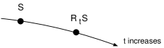
Figure 4: The RG transformation $R_{t}$ by scale $\mathrm{e}^{t}$ gives a flow in the space of all possible actions.

Along an RG flow, the correlation length changes trivially as

$$\xi(R_{t}S)=\mathrm{e}^{-t}\xi(S)$$

as a consequence of rescaling of space. This simple equation implies the following:

• If a theory is critical with $\xi=\infty$, it remains critical under RG.

• If a theory is non-critical, its correlation length becomes less and less along its RG flow.

2.2 Fixed points and relevant & irrelevant parameters

A fixed point is an action $S^{*}$ which is invariant under the RG transformation. At the fixed point we find

$$\left\langle\phi(\vec{r}_{1})\cdots\phi(\vec{r}_{n})\right\rangle_{S^{*}}=(1-n\gamma^{*}\Delta t)\left\langle\phi(\vec{r}_{1}\mathrm{e}^{-\Delta t})\cdots\phi(\vec{r}_{n}\mathrm{e}^{-\Delta t})\right\rangle_{S^{*}}$$

where

$$\gamma^{*}\equiv\gamma(S^{*})$$

Especially for $n=2$, we obtain

$$\left\langle\phi(\vec{r})\phi(-\vec{r})\right\rangle_{S^{*}}=\frac{\mathrm{const}}{r^{2\gamma^{*}}}\quad(r\gg 1)$$

This implies that the correlation length is infinite:

$$\xi\big{|}_{S^{*}}=+\infty$$

The scale transformation is compensated by renormalization of the field, and the physics at the fixed point $S^{*}$ is scale invariant with no characteristic length scale.

The scale dimension of the scalar field, $\gamma^{*}$, is not the only important quantity that characterizes the fixed point. To explain this, let us consider the RG flow in a small (but finite) neighborhood of $S^{*}$, where we expect to be able to linearize the RG transformation. Let

$$S[\phi]=S^{*}[\phi]+\delta S[\phi]$$

The RG transformation is given by

$$\partial_{t}\delta S[\phi]=L\cdot\delta S[\phi]$$

where $L$ is a linear transformation. We introduce eigenvectors of $L$ by

$$Lv_{i}[\phi]=y_{i}v_{i}[\phi]\quad(y_{1}\geq y_{2}\geq\cdots)$$

Using $v_{i}[\phi]$ we can expand the difference $\delta S[\phi]$:

$$\delta S[\phi]=\sum_{i=1}^{\infty}g_{i}(t)v_{i}[\phi]$$

Since the RG transformation is linearized in this basis, we obtain

$$\frac{d}{dt}g_{i}=c_{i}g_{i}\Longrightarrow g_{i}(t)\propto\mathrm{e}^{y_{i}t}$$

We can use the parameters $\{g_{i}\}$ as the coordinates of the theory space in the neighborhood of $S^{*}$. We call $g_{i}$ with positive eigenvalues $y_{i}>0$ relevant, and those with negative eigenvalues irrelevant. Like the scale dimension $\gamma^{*}$ of the scalar field, the scale dimensions of the relevant and irrelevant parameters characterize the fixed point $S^{*}$.

2.3 Critical subspace and renormalized trajectory

As an example, let us consider a fixed point $S^{*}$ with one relevant parameter $g_{1}$ with scale dimension $y_{1}>0$. All the other (an infinite number of them) parameters are irrelevant. Let $g_{2}$ be the least irrelevant, meaning that its scale dimension $y_{2}<0$ is the largest. In an infinitesimal neighborhood of $S^{*}$, it is a good approximation to keep just $g_{1}$ and $g_{2}$ satisfying the RG equations

$$\left\{\begin{array}[]{c@{~=~}l}\frac{d}{dt}g_{1}\hfil~{}=~{}&y_{1}\,g_{1}\\ \frac{d}{dt}g_{2}\hfil~{}=~{}&y_{2}\,g_{2}\end{array}\right.$$

The solution is easily obtained as

$$g_{1}(t)=g_{1}(0)\mathrm{e}^{y_{1}t},\quad g_{2}(t)=g_{2}(0)\mathrm{e}^{y_{2}t}$$

As $t$ grows, $g_{2}$ goes to $0$ while $g_{1}$ grows unless $g_{1}=0$ to begin with. All the other irrelevant parameters $g_{i\geq 3}$ approach zero faster than $g_{2}$.

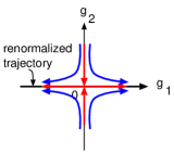
Figure 5: As $t$ grows, the irrelevant parameter $g_{2}$ decreases. The renormalized trajectory is the line $g_{2}=0$.

In the neighborhood of $S^{*}$, where $g_{1}$ is well defined, we can define a subspace by a single condition

$$\framebox{$\displaystyle g_{1}=0$}$$

This is called a critical subspace $\mathcal{S}_{cr}$. The critical subspace can be defined in a larger neighborhood of $S^{*}$ as the subspace which flows into the fixed point $S^{*}$ as $t\to+\infty$:

$$\lim_{t\to\infty}R_{t}\mathcal{S}_{cr}=S^{*}$$

This implies that the long-distance behavior of any theory in $\mathcal{S}_{cr}$ is the same as the fixed point $S^{*}$. Especially, for any theory on $\mathcal{S}_{cr}$, we find the correlation length infinite

$$\xi\big{|}_{\mathrm{on~{}}\mathcal{S}_{cr}}=+\infty$$

and the theory is critical. Given an arbitrary theory with $N$ parameters, what is the likelihood that the theory is critical? Since $\mathcal{S}_{cr}$ is defined by a single condition $g_{1}=0$, we expect that we need to fine tune only one of the $N$ parameters to make the theory critical.

Another subspace, called a renormalized trajectory $\mathcal{S}_{\infty}$, is defined by the vanishing of all the irrelevant parameters:

$$\framebox{$\displaystyle g_{2}=g_{3}=\cdots=0$}$$

This is a one-dimensional subspace with a single parameter $g_{1}$. Alternatively, $\mathcal{S}_{\infty}$ can be defined as the solution of the equation

$$(\forall t>0)\quad R_{t}\mathcal{S}_{\infty}=\mathcal{S}_{\infty}$$

implying that if $g_{1}$ is the coordinate of an arbitrary theory on $\mathcal{S}_{\infty}$, then $g_{1}\mathrm{e}^{-y_{1}t}$ also belongs to $\mathcal{S}_{\infty}$. $\mathcal{S}_{\infty}$ can be also defined as the RG flow coming out of the fixed point $S^{*}$. Note that along the renormalized trajectory, the correlation length is given by

$$\xi=c_{\pm}|g_{1}|^{-\frac{1}{y_{1}}}$$

where $c_{\pm}$ is a constant, and $\pm$ is for $\pm g_{1}>0$. $\mathcal{S}_{\infty}$ is a one-dimensional subspace in the infinite dimensional space. Hence, a theory with a finite number of parameters has no chance of lying in $\mathcal{S}_{\infty}$.

2.4 Example: $3$ dimensional $\phi^{4}$ theory

Let us now consider the $3$ dimensional $\phi^{4}$ theory defined by the action

$$S=\int_{p<1}\frac{1}{2}\phi(\vec{p})\phi(-\vec{p})\left(p^{2}+m_{0}^{2}\right)+\frac{\lambda_{0}}{4!}\int_{p_{i}<1\atop p_{1}+\cdots+p_{4}=0}\phi(\vec{p}_{1})\cdots\phi(\vec{p}_{4})$$

For simplicity, we assume that the theory lies in the subspace where we can linearize the RG transformation. Then, the coordinates $g_{i}$ are obtained as functions of $\lambda_{0}$ and $m_{0}^{2}$:

$$g_{i}=G_{i}(m_{0}^{2},\lambda_{0})\quad(i=1,2,\cdots)$$

For any $\lambda_{0}>0$, we only need to tune $m_{0}^{2}=m_{0,cr}^{2}(\lambda_{0})$ to make the theory critical. This implies that there is only one relevant parameter $g_{1}$, and $g_{i\geq 2}$ are all irrelevant. Hence, we obtain

$$G_{1}(m^{2}_{0,cr}(\lambda_{0}),\lambda_{0})=0$$

The critical exponents $y_{E},\eta$ introduced in the previous lecture are given by the scale dimensions $y_{1},\gamma^{*}$ of the fixed point $S^{*}$:

$$\left\{\begin{array}[]{c@{~=~}l}y_{E}\hfil~{}=~{}&y_{1}\\ \eta\hfil~{}=~{}&2\gamma^{*}-1\end{array}\right.$$

For a given $\lambda_{0}$, let us consider a theory near criticality:

$$m_{0}^{2}=m_{0,cr}^{2}(\lambda_{0})+\Delta m_{0}^{2}$$

Expanding $G_{i}$ with respect to $\Delta m_{0}^{2}$, we obtain

$$\begin{array}[]{c@{~=~}l}g_{1}\hfil~{}=~{}&\Delta m_{0}^{2}\frac{\partial G_{1}(m_{0}^{2},\lambda_{0})}{\partial m_{0}^{2}}\Big{|}_{m_{0}^{2}=m_{0,cr}^{2}}+\cdots\\ g_{i\geq 2}\hfil~{}=~{}&G_{i}(m_{0,cr}^{2}(\lambda_{0}),\lambda_{0})+\mathrm{O}\left(\Delta m_{0}^{2}\right)\end{array}$$

Applying $R_{t}$ for large $t\gg 1$, we obtain

$$\begin{array}[]{c@{~\simeq~}l}g_{1}(t)\hfil~{}\simeq~{}&\mathrm{e}^{y_{1}t}\Delta m_{0}^{2}\frac{1}{z_{m}(\lambda_{0})}\\ g_{i\geq 2}(t)\hfil~{}\simeq~{}&\mathrm{O}(\mathrm{e}^{y_{i}t})\end{array}$$

where

$$\frac{1}{z_{m}(\lambda_{0})}\equiv\left.\frac{\partial G_{1}(m_{0}^{2},\lambda_{0})}{\partial m_{0}^{2}}\right|_{m_{0}^{2}=m_{0,cr}^{2}(\lambda_{0})}$$

Hence, by choosing

$$\Delta m_{0}^{2}=z_{m}(\lambda_{0})\mathrm{e}^{-y_{1}t}c_{1}$$

for $t\gg 1$, we obtain

$$\left\{\begin{array}[]{c@{~\simeq~}l}g_{1}(t)\hfil~{}\simeq~{}&c_{1}\\ g_{i\geq 2}(t)\hfil~{}\simeq~{}&0\end{array}\right.$$

Thus, RG gives

$$\left\langle\phi(\vec{r}_{1}\mathrm{e}^{t})\cdots\phi(\vec{r}_{n}\mathrm{e}^{t})\right\rangle_{m_{0}^{2}=m_{0,cr}^{2}(\lambda_{0})+\Delta m_{0}^{2},\lambda_{0}}$$

$$= \exp\left[-n\int_{0}^{t}dt^{\prime}\gamma(R_{t^{\prime}}S)\right]\left\langle\phi(\vec{r}_{1})\cdots\phi(\vec{r}_{n})\right\rangle_{g_{1}=c_{1},~{}g_{i\geq 2}=0}$$

Defining

$$z(\lambda_{0})\equiv\exp\left[2\int_{0}^{\infty}dt\left\{\gamma\left(R_{t}S(m_{0,cr}^{2},\lambda_{0})\right)-\gamma^{*}\right\}\right]$$

we obtain

$$\left\langle\phi(\vec{r}_{1})\cdots\phi(\vec{r}_{n})\right\rangle_{g_{1}=c_{1},~{}g_{i\geq 2}=0}=z(\lambda_{0})^{\frac{n}{2}}\lim_{t\to\infty}\mathrm{e}^{n\gamma^{*}t}\left\langle\phi(\vec{r}_{1}\mathrm{e}^{t})\cdots\phi(\vec{r}_{n}\mathrm{e}^{t})\right\rangle_{m_{0}^{2},\lambda_{0}}$$

where

$$m_{0}^{2}=m_{0,cr}^{2}(\lambda_{0})+z_{m}(\lambda_{0})\mathrm{e}^{-y_{1}t}c_{1}$$

This reproduces the prescription introduced in the previous lecture.

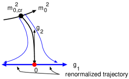
Figure 6: The RG flows starting from near the critical point $m_{0,cr}^{2}(\lambda_{0})$ approach the renormalized trajectories.

We now understand that the renormalized trajectory $\mathcal{S}_{\infty}$ corresponds to the renormalized theory viewed at different scales. As we have remarked already, it is practically impossible to construct an action on $\mathcal{S}_{\infty}$. However, the correlation functions on $\mathcal{S}_{\infty}$ can be obtained as the continuum limit of a theory only with a finite number of parameters such as $m_{0}^{2}$ and $\lambda_{0}$.

2.5 Three issues with renormalization

Let us now examine the three issues with renormalization with which we started this lecture.

1. how to renormalize a theory — we now understand why the prescription given in the first lecture gives the continuum limit.

2. universality — the renormalized theory is determined by the renormalized trajectory. Hence, it is independent of $\lambda_{0}$. We can go further. Even if we start from an action with other interactions such as the $\phi^{6}$ interaction, as long as the critical theory lies on the same $\mathcal{S}_{cr}$, we get the same continuum limit. As an extreme case, we get the same limit from the Ising model.

3. finite number of parameters — the number of renormalized parameters is determined by the dimensionality of $\mathcal{S}_{\infty}$, which is the number of relevant parameters.

Thus, we understand that for each fixed point $S^{*}$ and the associated renormalized trajectory $\mathcal{S}_{\infty}$, we can construct a renormalized theory.

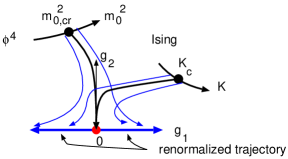
Figure 7: As long as the critical point belongs to the same critical subspace $\mathcal{S}_{cr}$, we get the same continuum limit.

3 Lecture 3 – Perturbative Exact RG

It was Joe Polchinski who first applied Wilson’s RG to the perturbative $\phi^{4}$ theory in $4$ dimensions in order to “simplify” the proof of renormalizability.[4] His proof was simple in the sense that it did not rely on the analysis of Feynman graphs or Feynman integrals. I quoted the word “simple”, though, because even his proof is not what I would recommend first year grad students to go through.

We recall that Wilson’s RG consists of three steps: integration of momenta near the cutoff, rescaling of space, and renormalization of field. The second and third steps are crucial for the RG transformation to have fixed points. For applications to perturbation theory, however, only the first step is important, since there is no non-trivial fixed point in perturbation theory. Hence, we define the exact RG only by the first step, namely the lowering of the momentum cutoff.

We consider a real scalar theory in $4$ dimensions in this lecture, and QED in the next lecture. We define the scalar theory by the following action:

$$S(t)=\left.\frac{1}{2}\int_{p}\phi(p)\phi(-p)\frac{p^{2}+m^{2}}{K\left(\frac{p}{\mu\mathrm{e}^{-t}}\right)}\right\}=S_{free}(t)$$

$$~{}\left.-\sum_{n=1}^{\infty}\frac{1}{(2n)!}\int_{p_{1}+\cdots+p_{2n}=0}\mathcal{V}_{2n}(t;p_{1},\cdots,p_{2n})\phi(p_{1})\cdots\phi(p_{2n})\right\}=S_{int}(t)$$

where we have omitted the tilde from the Fourier modes. The function $K(x)$ has the property that it is $1$ for $0\leq x\leq 1$ and converges rapidly to $0$ as $x\to\infty$.

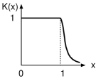
Figure 8: The cutoff function $K(x)$ decreases rapidly in the region $x>1$.

Hence, effectively the scalar field has the momentum cutoff

$$\framebox{$\displaystyle\Lambda=\mu\mathrm{e}^{-t}$}$$

Please note that we have chosen a sign convention for $t$ so that $\Lambda$ decreases as we increase $t$. The interaction vertices $\mathcal{V}_{2n}$ depend on momenta, and we treat them perturbatively, using

$$\framebox{$\displaystyle\frac{K\left(\frac{p}{\mu\mathrm{e}^{-t}}\right)}{p^{2}+m^{2}}$}$$

as the propagator. Denoting the interaction vertices as

a typical Feynman graph would look like

Since the loop momenta are cut off at $p=\mu\mathrm{e}^{-t}$, there is no UV divergences.

3.1 Derivation of ERG differential equations

We define ERG by the change of the action under the decrease of $\Lambda$ or equivalently the increase of $t$. We change the action in such a way that the correlation functions do not change.

$$\left\langle\phi(\vec{p}_{1})\cdots\phi(\vec{p}_{2n})\right\rangle_{S(t)}=\left\langle\phi(\vec{p}_{1})\cdots\phi(\vec{p}_{2n})\right\rangle_{S(t+\Delta t)}$$

where $\Delta t>0$ and

$$(\forall i)\quad p_{i}<\mu\mathrm{e}^{-t-\Delta t}$$

This can be done by compensating the change of the propagator by changing the vertices, as we will see shortly.

In calculating the correlation functions, a propagator acts in one of the three ways:

1. it connects two distinct vertices (internal line)

2. it connects the same vertex (internal line)

3. it is attached to an external source (external line)

Now, as we increase $t$ infinitesimally to $t+\Delta t$, we find

$$K\left(\frac{p}{\mu\mathrm{e}^{-t}}\right)=K\left(\frac{p}{\mu\mathrm{e}^{-t-\Delta t}}\right)+\Delta t\underbrace{(-)\frac{\partial}{\partial t}K\left(\frac{p}{\mu\mathrm{e}^{-t}}\right)}_{\equiv\Delta\left(\frac{p}{\mu\mathrm{e}^{-t}}\right)}$$

Hence, denoting

$\displaystyle\frac{\Delta\left(\frac{p}{\mu\mathrm{e}^{-t}}\right)}{p^{2}+m^{2}}=$

we obtain

$\displaystyle\frac{K\left(\frac{p}{\mu\mathrm{e}^{-t}}\right)}{p^{2}+m^{2}}=\frac{K\left(\frac{p}{\mu\mathrm{e}^{-t-\Delta t}}\right)}{p^{2}+m^{2}}+\Delta t$

Let us consider a Feynman diagram for the action $S(t)$. The propagator is given by the left-hand side above. Imagine replacing the propagator by the right-hand side and expand the diagram in powers of $\Delta t$. At first order in $\Delta t$, we must use the second term (red line) just once. It enters the Feynman graph in one of the two ways shown in Figure 8,

Figure 9: Two types of corrections to $S_{int}$

We don’t have to consider a red line attached to an external source, if we restrict all the external momenta by $p<\mu\mathrm{e}^{-t-\Delta t}$.

Incorporating the contribution of the red line as part of a vertex, we obtain the following diagrammatic differential equation:

$\displaystyle\frac{\partial}{\partial t}\mathcal{V}_{2n}(t;p_{1},\cdots,p_{2n})=$

$+$

The first term on the right is actually a sum over all possible partitions of $2n$ external momenta into two parts. This can be expressed nicely using a more abstract notation as

$$\partial_{t}(-S_{int})(t)=\frac{1}{2}\int_{p}\frac{\Delta\left(\frac{p}{\mu\mathrm{e}^{-t}}\right)}{p^{2}+m^{2}}\left[\frac{\delta(-S_{int})(t)}{\delta\phi(p)}\frac{\delta(-S_{int})(t)}{\delta\phi(-p)}+\frac{\delta^{2}(-S_{int})(t)}{\delta\phi(p)\delta\phi(-p)}\right]$$

Problem 3-1: Check this result.
These differential equations for the vertices, which we call perturbative ERG differential equations, were derived by Polchinski.[4]

3.2 Renormalization

As is the case with any differential equations, we must specify initial conditions to solve the ERG differential equations. To obtain the renormalized trajectories or equivalently the continuum limit, we need to take the theory to criticality, as we saw in the previous lectures. Thanks to universality, it does not matter what initial conditions to choose as long as we can tune them for criticality. For example, we can choose the initial condition at $t=t_{0}$ in the following form:

$$\left\{\begin{array}[]{r@{~=~}l}\mathcal{V}_{2}(t_{0};p,-p)~{}=~{}&\mu^{2}\mathrm{e}^{-2t_{0}}g(\lambda,t_{0})+m^{2}z_{m}(\lambda,t_{0})+p^{2}z(\lambda,t_{0})\\ \mathcal{V}_{4}(t_{0};p_{1},\cdots,p_{4})~{}=~{}&-\lambda(1+z_{\lambda}(\lambda,t_{0}))\\ \mathcal{V}_{2n\geq 6}(t_{0};p_{1},\cdots,p_{2n})~{}=~{}&0\end{array}\right.$$

We determine $g(\lambda,t_{0})$ so that the theory is critical at $m^{2}=0$. In perturbation theory, we determine the functions $g,z_{m},z$, and $z_{\lambda}$ as power series in $\lambda$ so that the vertices $\{\mathcal{V}_{2n}(t)\}$, for any finite $t$, are well defined in the limit $t_{0}\to-\infty$. This is how renormalizability was proved in ref. [4].

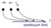
Figure 10: The continuum limit is obtained as $t_{0}\to-\infty$.

3.3 Asymptotic conditions

In the previous lecture we have mentioned that it is practically impossible to construct the actions on the renormalized trajectories, even though we can construct the continuum limit of the correlation functions. In perturbation theory, however, this can be done by solving the ERG differential equations under appropriate conditions.

The $\phi^{4}$ theory does not have the kind of fixed point that the three dimensional sibling has. Hence, we cannot demand that the renormalized trajectories trace back to a fixed point as we go backward along ERG. Instead, we can demand that the renormalized trajectories satisfy the following asymptotic conditions as $t\to-\infty$:[7]

$$\left\{\begin{array}[]{r@{~\longrightarrow~}l}\mathcal{V}_{2}(t;p,-p)~{}\longrightarrow~{}&\mu^{2}\mathrm{e}^{-2t}a_{2}(t;\lambda)+m^{2}b_{2}(t;\lambda)+p^{2}c_{2}(t;\lambda)\\ \mathcal{V}_{4}(t;p_{1},\cdots,p_{4})~{}\longrightarrow~{}&a_{4}(t;\lambda)\\ \mathcal{V}_{2n\geq 6}(t;p_{1},\cdots,p_{2n})~{}\longrightarrow~{}&\mathrm{O}(\mathrm{e}^{y_{2n}t})\end{array}\right.$$

Here, $a_{2},b_{2},c_{2}$, and $a_{4}$ are all power series of $\lambda$, and at each order of $\lambda$ they are polynomials of $t$. The $t$-independent part of $b_{2},c_{2},a_{4}$ are not fixed by ERG, and we can adopt the following convention:

$$\framebox{$\displaystyle\left\{\begin{array}[]{l}b_{2}(0;\lambda)=c_{2}(0;\lambda)=0\\ a_{4}(0;\lambda)=-\lambda\end{array}\right.$}$$

Hence, at first order in $\lambda$ we obtain

$$\mathcal{V}_{4}^{(1)}=-\lambda$$

This plays the role of a seed for perturbative expansions. The vertices are uniquely determined with $m^{2}$ and $\lambda$ as parameters.

As an example, let us determine the $2$-point vertex at first order. It satisfies

$$\partial_{t}\mathcal{V}_{2}^{(1)}(t;p,-p)=\frac{1}{2}\int_{q}\frac{\Delta\left(\frac{q}{\mu\mathrm{e}^{-t}}\right)}{q^{2}+m^{2}}\underbrace{\mathcal{V}_{4}^{(1)}(t;q,-q,p,-p)}_{=-\lambda}=-\frac{\lambda}{2}\int_{q}\frac{\Delta\left(\frac{q}{\mu\mathrm{e}^{-t}}\right)}{q^{2}+m^{2}}$$

For large $-t\gg 1$ we obtain

$$\int_{q}\frac{\Delta\left(\frac{q}{\mu\mathrm{e}^{-t}}\right)}{q^{2}+m^{2}}=\mu^{2}\mathrm{e}^{-2t}\int_{q}\frac{\Delta(q)}{q^{2}+\frac{m^{2}}{\mu^{2}\mathrm{e}^{-2t}}}\simeq\mu^{2}\mathrm{e}^{-2t}\int_{q}\frac{\Delta(q)}{q^{2}}-m^{2}\int_{q}\frac{\Delta(q)}{q^{4}}$$

Hence, we obtain

$$\mathcal{V}_{2}^{(1)}(t) = \frac{-\lambda}{2}\Bigg{[}\int_{-\infty}^{t}dt^{\prime}\int_{q}\Delta\left(\frac{q}{\mu\mathrm{e}^{-t^{\prime}}}\right)\underbrace{\left(\frac{1}{q^{2}+m^{2}}-\frac{1}{q^{2}}+\frac{m^{2}}{q^{4}}\right)}_{=\frac{m^{4}}{q^{4}(q^{2}+m^{2})}}$$

$$\quad-\frac{\mu^{2}\mathrm{e}^{-2t}}{2}\int_{q}\frac{\Delta(q)}{q^{2}}-tm^{2}\int_{q}\frac{\Delta(q)}{q^{4}}\Bigg{]}$$

$$= \frac{-\lambda}{2}\Bigg{[}\int_{q}\left(1-K\left(\frac{q}{\mu\mathrm{e}^{-t}}\right)\right)\frac{m^{4}}{q^{4}(q^{2}+m^{2})}$$

$$\quad\quad\quad-\frac{\mu^{2}\mathrm{e}^{-2t}}{2}\int_{q}\frac{\Delta(q)}{q^{2}}-tm^{2}\int_{q}\frac{\Delta(q)}{q^{4}}\Bigg{]}$$

This implies

$$\left\{\begin{array}[]{c@{~=~}l}a_{2}^{(1)}(t)\hfil~{}=~{}&\frac{\lambda}{4}\int_{q}\frac{\Delta(q)}{q^{2}}\\ b_{2}^{(1)}(t)\hfil~{}=~{}&\frac{\lambda}{2}t\int_{q}\frac{\Delta(q)}{q^{4}}=\lambda t\frac{1}{(4\pi)^{2}}\end{array}\right.$$

Problem 3-2: Compute $\mathcal{V}_{2}^{(1)}(t)$ explicitly for the choice $K(x)=\theta(1-x)$.
Problem 3-3: Using $\mathcal{V}_{2}^{(1)}(t)$ obtained above, compute the self-energy correction at first order. (Answer:

$$\frac{-\lambda}{2}\int_{q<\mu\mathrm{e}^{-t}}\frac{1}{q^{2}+m^{2}}+\mathcal{V}_{2}^{(1)}(t)=\frac{-\lambda}{(4\pi)^{2}}m^{2}\ln\frac{m^{2}}{\mu^{2}}\quad)$$

3.4 Diagrammatic rules

The vertices $\mathcal{V}_{2n}(t;p_{1},\cdots,p_{2n})$ are most easily calculated diagrammatically. Consider a Feynman diagram with the standard propagator, which we can decompose into the low and high momentum parts:

$$\frac{1}{p^{2}+m^{2}}=\frac{K\left(\frac{p}{\mu\mathrm{e}^{-t}}\right)}{p^{2}+m^{2}}+\frac{1-K\left(\frac{p}{\mu\mathrm{e}^{-t}}\right)}{p^{2}+m^{2}}$$

Substituting this into each propagator of a Feynman diagram, we get a bunch of diagrams in which low and high momentum propagators are mixed. By interpreting high momentum propagators not as propagators but as part of vertices, we get Feynman diagrams only with low momentum propagators.

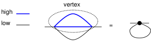
Figure 11: We interpret high momentum propagators as part of vertices.

Hence, the vertices are basically obtained from Feynman diagrams in which the propagator is given by the high-momentum propagator. The necessary UV subtractions are made in the BPHZ manner, i.e., at the level of integrands we subtract the first couple of terms of the Taylor series in $m^{2}$ and external momentum $p$. We then add finite counterterms to assure the correct $t$ dependence.

As an example, let us compute $\mathcal{V}_{4}$ at second order in $\lambda$. In the s-channel, we have

$\displaystyle=\frac{\lambda^{2}}{2}\int_{q}\frac{\left(1-K\left(\frac{q}{\mu\mathrm{e}^{-t}}\right)\right)\left(1-K\left(\frac{q+p}{\mu\mathrm{e}^{-t}}\right)\right)}{(q^{2}+m^{2})((q+p)^{2}+m^{2})}$

As it is, this is UV divergent. We subtract the integrand evaluated at $p^{2}=m^{2}=0$ to obtain a finite integral:

$$\frac{\lambda^{2}}{2}\int_{q}\left[\frac{\left(1-K\left(\frac{q}{\mu\mathrm{e}^{-t}}\right)\right)\left(1-K\left(\frac{q+p}{\mu\mathrm{e}^{-t}}\right)\right)}{(q^{2}+m^{2})((q+p)^{2}+m^{2})}-\frac{\left(1-K\left(\frac{q}{\mu\mathrm{e}^{-t}}\right)\right)^{2}}{q^{4}}\right]$$

But this does not have the correct $t$-dependence, and we must add a finite counterterm:

$$\lambda^{2}t\,\int_{q}\frac{\Delta\left(\frac{q}{\mu\mathrm{e}^{-t}}\right)\left(1-K\left(\frac{q}{\mu\mathrm{e}^{-t}}\right)\right)}{q^{4}}=\lambda^{2}t\,\int_{q}\frac{\Delta(q)(1-K(q))}{q^{4}}=\lambda^{2}t\frac{1}{(4\pi)^{2}}$$

Another type of contribution to $\mathcal{V}_{4}$ comes from the following 1PR (one-particle reducible) diagram:

$\displaystyle=\mathcal{V}_{2}^{(1)}(t)\frac{1-K\left(\frac{p_{1}}{\mu\mathrm{e}^{-t}}\right)}{p_{1}^{2}+m^{2}}(-\lambda)$

3.5 Beta function and anomalous dimensions

How do the beta function and anomalous dimensions arise in the context of ERG? To understand this, we first note that besides $t$ the action $S(t)$ has only $m^{2},\lambda$, and $\mu$ as parameters. The correlation functions are independent of $t$, and hence we can use the notation

$$\left\langle\phi(\vec{p}_{1})\cdots\phi(\vec{p}_{2n})\right\rangle_{m^{2},\lambda;\mu}$$

This can be calculated using any action $S(t)$ as long as $(\forall i)~{}\mu\mathrm{e}^{-t}>p_{i}$.

The beta function $\beta(\lambda)$ and anomalous dimensions $\beta_{m}(\lambda),\gamma(\lambda)$ describe the $\mu$ dependence of the correlation functions. For $\Delta t$ infinitesimal, we find

$$\left\langle\phi(\vec{p}_{1})\cdots\phi(\vec{p}_{2n})\right\rangle_{m^{2}(1-\Delta t\beta_{m}(\lambda)),\lambda-\Delta t\beta(\lambda);\mu(1+\Delta t)}$$

$$= \left(1-\Delta t\cdot 2n\gamma(\lambda)\right)\left\langle\phi(\vec{p}_{1})\cdots\phi(\vec{p}_{2n})\right\rangle_{m^{2},\lambda;\mu}$$

The beta function and anomalous dimensions are given in terms of asymptotic vertices defined by the following behavior as $t\to-\infty$:

$$\left\{\begin{array}[]{c@{~\longrightarrow~}l}\mathcal{V}_{4}(t;q\mu\mathrm{e}^{-t},-q\mu\mathrm{e}^{-t},p,-p)\hfil~{}\longrightarrow~{}&a_{4}(t;q)+\frac{m^{2}}{\mu^{2}\mathrm{e}^{-2t}}b_{4}(t;q)+\frac{p^{2}}{\mu^{2}\mathrm{e}^{-2t}}c_{4}(t;q)\\ \mathcal{V}_{6}(t;q\mu\mathrm{e}^{-t},-q\mu\mathrm{e}^{-t},0,0,0,0)\hfil~{}\longrightarrow~{}&\frac{1}{\mu^{2}\mathrm{e}^{-2t}}a_{6}(t;q)\end{array}\right.$$

Then, we obtain

$$2\gamma(\lambda) = \frac{-\frac{1}{2}\int_{q}\frac{\Delta(q)}{q^{2}}c_{4}(0;q)}{1-\frac{1}{2}\int_{q}\frac{K(q)(1-K(q))}{q^{4}}c_{4}(0;q)}$$

$$\beta_{m}(\lambda) = \frac{1}{1-\frac{1}{2}\int_{q}\frac{K(q)(1-K(q))}{q^{2}}a_{4}(0;q)}\Bigg{[}\frac{1}{2}\int_{q}\Delta(q)\left(\frac{a_{4}(0;q)}{q^{4}}-\frac{b_{4}(0;q)}{q^{2}}\right)$$

$$\quad-2\gamma(\lambda)\left\{1+\frac{1}{2}\int_{q}K(q)(1-K(q))\left(\frac{a_{4}(0;q)}{q^{4}}-\frac{b_{4}(0;q)}{q^{2}}\right)\right\}\Bigg{]}$$

$$\beta(\lambda) = -\frac{1}{2}\int_{q}\frac{\Delta(q)}{q^{2}}a_{6}(0;q)-2\gamma(\lambda)\left(2\lambda-\frac{1}{2}\int_{q}\frac{K(q)(1-K(q))}{q^{2}}a_{6}(0;q)\right)$$

These get much simplified for the particular choice:

$$K(q)=\theta(1-q)$$

Problem 3-4: Simplify the formulas for the beta function and anomalous dimensions for the above choice of $K$. (Note $K(1-K)=0$.)

To lowest order in $\lambda$, we find

$$\left\{\begin{array}[]{c@{~=~}l}a_{4}(0;q)\hfil~{}=~{}&-\lambda+\mathrm{O}(\lambda^{2})\\ b_{4}(0;q)\hfil~{}=~{}&\mathrm{O}(\lambda^{2})\\ c_{4}(0;q)\hfil~{}=~{}&\mathrm{O}(\lambda^{2})\\ a_{6}(0;q)\hfil~{}=~{}&6\lambda^{2}\frac{1-K(q)}{q^{2}}+\mathrm{O}(\lambda^{3})\end{array}\right.$$

and we obtain the familiar results:

$$\left\{\begin{array}[]{c@{~=~}l}\gamma(\lambda)\hfil~{}=~{}&\mathrm{O}(\lambda^{2})\\ \beta_{m}(\lambda)\hfil~{}=~{}&\frac{1}{2}\int_{q}\frac{\Delta(q)}{q^{4}}(-\lambda)+\mathrm{O}(\lambda^{2})\simeq-\frac{\lambda}{(4\pi)^{2}}\\ \beta(\lambda)\hfil~{}=~{}&-\frac{1}{2}\int_{q}\frac{\Delta(q)}{q^{2}}6\lambda^{2}\frac{1-K(q)}{q^{2}}+\mathrm{O}(\lambda^{3})\simeq-\frac{3\lambda^{2}}{(4\pi)^{2}}\end{array}\right.$$

4 Lecture 4 – Application to QED

To define QED we must introduce a vector field $A_{\mu}$ for photons and a spinor field $\psi$ for electrons. The free part of the action is given by

$$S_{free}(t)=\frac{1}{2}\int_{k}A_{\mu}(k)A_{\nu}(-k)\frac{k^{2}\delta_{\mu\nu}-\left(1-\frac{1}{\xi}\right)k_{\mu}k_{\nu}}{K\left(\frac{k}{\mu\mathrm{e}^{-t}}\right)}+\int_{p}\bar{\psi}(-p)\frac{\hbox{$p$\kern-5.0pt\raise 1.29167pt\hbox{/}}+im}{K\left(\frac{p}{\mu\mathrm{e}^{-t}}\right)}\psi(p)$$

so that the propagators are given by

$\displaystyle=\frac{K\left(\frac{k}{\mu\mathrm{e}^{-t}}\right)}{k^{2}}\left(\delta_{\mu\nu}-(1-\xi)\frac{k_{\mu}k_{\nu}}{k^{2}}\right)$

$\displaystyle=\frac{K\left(\frac{p}{\mu\mathrm{e}^{-t}}\right)}{\hbox{$p$\kern-5.0pt\raise 1.29167pt\hbox{/}}+im}$

We write the interaction part of the action as

$$S_{int}(t)=-\sum_{M=1}^{\infty}\sum_{N=1}^{\infty}\frac{1}{M!}\frac{1}{(N!)^{2}}\int_{k_{1}+\cdots+p_{N}=0}$$

$$~{}A_{\mu_{1}}(k_{1})\cdots A_{\mu_{M}}(k_{M})\bar{\psi}(-q_{1})\cdots\bar{\psi}(-q_{N})$$

$$~{}\cdot\mathcal{V}_{\mu_{1}\cdots\mu_{M},N}(-t;k_{1},\cdots,k_{M};-q_{1},\cdots,-q_{N};p_{1},\cdots,p_{N})\psi(p_{1})\cdots\psi(p_{N})$$

We can denote the vertices graphically as

$\displaystyle\mathcal{V}_{\mu_{1},\cdots,\mu_{M},N}(t;k_{1},\cdots,-q_{1},\cdots,p_{1},\cdots)=$

The vertices satisfy the ERG differential equations given graphically by

$\displaystyle\frac{\partial}{\partial t}$

$\displaystyle=$

$\displaystyle+$

$\displaystyle+$

$\displaystyle+$

where

$\displaystyle=\frac{\Delta\left(\frac{k}{\mu\mathrm{e}^{-t}}\right)}{k^{2}}\left(\delta_{\mu\nu}-(1-\xi)\frac{k_{\mu}k_{\nu}}{k^{2}}\right)$

$\displaystyle=\frac{\Delta\left(\frac{p}{\mu\mathrm{e}^{-t}}\right)}{\hbox{$p$\kern-5.0pt\raise 1.29167pt\hbox{/}}+im}$

The theory is obtained by solving the ERG differential equations under the following asymptotic conditions for $t\to-\infty$:

$$\mathcal{V}_{\mu\nu}(t;k,-k) \longrightarrow \delta_{\mu\nu}\left(\mu^{2}\mathrm{e}^{-2t}a_{2}(t)+m^{2}b_{2}(t)\right)$$

$$~{}+k^{2}\delta_{\mu\nu}c_{2}(t)+k_{\mu}k_{\nu}d_{2}(t)$$

$$\mathcal{V}_{1}(t;p,-p) \longrightarrow a_{f}(t)\hbox{$p$\kern-5.0pt\raise 1.29167pt\hbox{/}}+b_{f}(t)im$$

$$\mathcal{V}_{\mu,1}(t;k,-p-k,p) \longrightarrow a_{3}(t)\gamma_{\mu}$$

$$\mathcal{V}_{\alpha\beta\gamma\delta}(t;k_{1},\cdots,k_{4}) \longrightarrow a_{4}(t)\left(\delta_{\alpha\beta}\delta_{\gamma\delta}+\delta_{\alpha\gamma}\delta_{\beta\delta}+\delta_{\alpha\delta}\delta_{\beta\gamma}\right)$$

$$\mathrm{higher~{}vertices} \longrightarrow 0$$

Note that the three-point vertex of photons vanish identically

$$\mathcal{V}_{\alpha\beta\gamma}=0$$

since we impose invariance under charge conjugation.

In specifying the asymptotic conditions, all the $t$-dependence of the asymptotic vertices are fixed by the ERG differential equations. But

$$b_{2}(0),~{}c_{2}(0),~{}d_{2}(0),~{}a_{f}(0),~{}b_{f}(0),~{}a_{3}(0),~{}a_{4}(0)$$

are free parameters, and we can take them arbitrarily as far as renormalization is concerned. We can choose

$$c_{2}(0)=a_{f}(0)=0$$

by normalizing the fields $A_{\mu},\psi$ appropriately. We can also take

$$b_{f}(0)=0$$

by normalizing the mass parameter $m$ of the electron appropriately. We could choose $a_{3}(0)=e$, the electric charge, but we prefer to introduce $e$ through the Ward identities. In the following we will show that

$$b_{2}(0),~{}d_{2}(0),~{}a_{3}(0),~{}a_{4}(0)$$

are determined uniquely as power series of $e$ by imposing that the theory satisfy the Ward identities.

4.1 Ward identities

Let us recall the Ward identities. The two-point function of the gauge field satisfies

$$\frac{1}{\xi}k_{\mu}\left\langle A_{\mu}(-k)A_{\nu}(k)\right\rangle=\frac{k_{\nu}}{k^{2}}$$

and those with electron fields satisfy

$$\frac{1}{\xi}k_{\mu}\left\langle A_{\mu}(-k)A_{\mu_{1}}\cdots A_{\mu_{M}}(k_{M})\psi(q_{1})\cdots\psi(q_{N})\bar{\psi}(-p_{1})\cdots\bar{\psi}(-p_{N})\right\rangle$$

$$= \frac{e}{k^{2}}\sum_{n=1}^{N}\left(\left\langle A_{\mu_{1}}\cdots\psi(q_{n}-k)\cdots\right\rangle-\left\langle A_{\mu_{1}}\cdots\bar{\psi}(-p_{n}-k)\cdots\right\rangle\right)$$

These Ward identities are expected to imply the invariance of the action under gauge transformations or the BRST transformation. The Ward identities imply

1. that the photon has only two transverse degrees of freedom,

2. that the S-matrix is independent of the gauge fixing parameter $\xi$.

There is a complication, however, since our action

$$S(t)=S_{free}(t)+S_{int}(t)$$

gives the correlation functions correctly only for external momenta less than $\mu\mathrm{e}^{-t}$. This calls for two changes:

1. We must modify the BRST transformation.

2. The action is not strictly invariant under the modified BRST transformation.

The derivation would take too much space and time (one full lecture; see ref. [8]), and we will content ourselves by merely describing the results.

4.1.1 Modified BRST transformation

We generalize the action by including Faddeev-Popov ghost and antighost fields:

$$S_{free}(t) = \frac{1}{2}\int_{k}A_{\mu}(-k)A_{\nu}(k)\frac{k^{2}\delta_{\mu\nu}-\left(1-\frac{1}{\xi}\right)k_{\mu}k_{\nu}}{K\left(\frac{k}{\mu\mathrm{e}^{-t}}\right)}$$

$$\quad+\int_{p}\bar{\psi}(-p)\frac{\hbox{$p$\kern-5.0pt\raise 1.29167pt\hbox{/}}+im}{K\left(\frac{p}{\mu\mathrm{e}^{-t}}\right)}\psi(p)+\int_{k}\bar{c}(-k)\frac{k^{2}}{K\left(\frac{k}{\mu\mathrm{e}^{-t}}\right)}c(k)$$

where $c$ and $\bar{c}$ are both anticommuting fields. The interaction part of the action is free of $c,\bar{c}$. We then introduce the following BRST transformation:

$$\left\{\begin{array}[]{c@{~=~}l}\delta_{\epsilon}A_{\mu}(k)\hfil~{}=~{}&k_{\mu}\epsilon~{}c(k)\\ \delta_{\epsilon}c(k)\hfil~{}=~{}&0\\ \delta_{\epsilon}\bar{c}(-k)\hfil~{}=~{}&-\frac{1}{\xi}k_{\mu}A_{\mu}(-k)\epsilon\\ \delta_{\epsilon}\psi(p)\hfil~{}=~{}&e\int_{k}\epsilon~{}c(k)\frac{K\left(\frac{p}{\mu\mathrm{e}^{-t}}\right)}{K\left(\frac{p-k}{\mu\mathrm{e}^{-t}}\right)}\psi(p-k)\\ \delta_{\epsilon}\bar{\psi}(-p)\hfil~{}=~{}&-e\int_{k}\epsilon~{}c(k)\frac{K\left(\frac{p}{\mu\mathrm{e}^{-t}}\right)}{K\left(\frac{p+k}{\mu\mathrm{e}^{-t}}\right)}\bar{\psi}(-p-k)\end{array}\right.$$

where $\epsilon$ is an arbitrary anticommuting constant. In the limit $t\to-\infty$, we find $K=1$, and the above reduces to the standard BRST transformation.

4.1.2 BRST transformation of the action

The total action $S(t)=S_{free}(t)+S_{int}(t)$ is not quite BRST invariant. It must transform as

$$\delta_{\epsilon}S(t)=-\int_{k}\epsilon~{}c(k)\mathcal{O}(t;-k)$$

where

$$\mathcal{O}(t;-k) \equiv \int_{p}\Bigg{[}\frac{\overrightarrow{\delta}}{\delta\bar{\psi}_{i}(-p)}\left(-S(t)\right)\cdot\left(-S(t)\right)\frac{\overleftarrow{\delta}}{\delta\psi_{j}(p+k)}$$

$$+\frac{\overrightarrow{\delta}}{\delta\bar{\psi}_{i}(-p)}\left(-S(t)\right)\frac{\overleftarrow{\delta}}{\delta\psi_{j}(p+k)}\Bigg{]}U_{ji}(t;-p-k,p)$$

and

$$U(t;-p-k,p)\equiv e\left\{K\left(\frac{p+k}{\mu\mathrm{e}^{-t}}\right)\frac{1-K\left(\frac{p}{\mu\mathrm{e}^{-t}}\right)}{\hbox{$p$\kern-5.0pt\raise 1.29167pt\hbox{/}}+im}-\frac{1-K\left(\frac{p+k}{\mu\mathrm{e}^{-t}}\right)}{\hbox{$p$\kern-5.0pt\raise 1.29167pt\hbox{/}}+\hbox{$k$\kern-5.0pt\raise 1.29167pt\hbox{/}}+im}K\left(\frac{p}{\mu\mathrm{e}^{-t}}\right)\right\}$$

The above BRST transformation property guarantees the Ward identities of the correlation functions for external momenta less than the cutoff $\mu\mathrm{e}^{-t}$. It also has the important property that if it is satisfied at some $t$, the ERG differential equation implies that it is satisfied at any other $t$. Hence, the BRST transformation property is consistent with the ERG.

4.1.3 BRST invariance at $t\to-\infty$

The consistency of the BRST “invariance” or transformation property of the action $S(t)$ with ERG implies that we only need to check it asymptotically as $t\to-\infty$. If it is satisfied asymptotically, it is satisfied for any finite $t$. As $t\to-\infty$,

$$\delta_{\epsilon}S(t)=-\int_{k}\epsilon~{}c(k)\mathcal{O}(t;-k)$$

gives the following three equations.

$\displaystyle k_{\mu}\left(\mu^{2}\mathrm{e}^{-2t}a_{2}(t)+m^{2}b_{2}(t)+k^{2}(c_{2}+d_{2})(t)\right)=-\lim_{t\to-\infty}$

$\displaystyle a_{3}(t)\hbox{$k$\kern-5.0pt\raise 1.29167pt\hbox{/}}=e\left(1-a_{f}(t)\right)\hbox{$k$\kern-5.0pt\raise 1.29167pt\hbox{/}}-\lim_{t\to-\infty}$

$\displaystyle a_{4}(t)\left(k_{\alpha}\delta_{\beta\gamma}+k_{\beta}\delta_{\gamma\alpha}+k_{\gamma}\delta_{\alpha\beta}\right)=-\lim_{t\to-\infty}$

where

$\displaystyle=U(t;-p-k,p)$

For the higher point vertices, we simply get $0=0$. From the second equation, we immediately see

$$\framebox{$\displaystyle a_{3}(0)=e+\mathrm{O}(e^{3})$}$$

It is clear that the above BRST transformation properties determine the coefficients $b_{2}(0),d_{2}(0),a_{3}(0),a_{4}(0)$ uniquely if we use the convention $c_{2}(0)=a_{f}(0)=0$.

4.2 One-loop calculations

Let us compute $b_{2}(0),d_{2}(0),a_{3}(0)-e,a_{4}(0)$ at one-loop.

4.2.1 Photon two-point

At one-loop, we obtain

$-$

$\displaystyle=e^{2}\int_{q}$

$\displaystyle\times\mathrm{Sp}~{}\left[\gamma_{\nu}\left(K\left(\frac{q+k}{\mu\mathrm{e}^{-t}}\right)\frac{1-K\left(\frac{q}{\mu\mathrm{e}^{-t}}\right)}{\hbox{$q$\kern-5.0pt\raise 1.29167pt\hbox{/}}+im}-\frac{1-K\left(\frac{q+k}{\mu\mathrm{e}^{-t}}\right)}{\hbox{$q$\kern-5.0pt\raise 1.29167pt\hbox{/}}+\hbox{$k$\kern-5.0pt\raise 1.29167pt\hbox{/}}+im}K\left(\frac{q}{\mu\mathrm{e}^{-t}}\right)\right)\right]$

$$\stackrel{{\scriptstyle t\to\infty}}{{\longrightarrow}}e^{2}k_{\nu}\left[-2\mu^{2}\mathrm{e}^{-2t}\int_{q}\frac{\Delta(q)(1-K(q))}{q^{2}}+\left(m^{2}+\frac{1}{3}k^{2}\right)\int_{q}\frac{\Delta(q)}{q^{4}}\right]$$

Thus, we obtain

$$\left\{\begin{array}[]{c@{~=~}l}b_{2}(0)\hfil~{}=~{}&e^{2}\int_{q}\frac{\Delta(q)}{q^{4}}=\frac{2e^{2}}{(4\pi)^{2}}\\ c_{2}(0)\hfil~{}=~{}&\frac{e^{2}}{3}\int_{q}\frac{\Delta(q)}{q^{4}}=\frac{4e^{2}}{3(4\pi)^{2}}\end{array}\right.$$

(In fact $b_{2}(t)$ is independent of $t$.)

4.2.2 Photon-electron vertex

At one-loop, we obtain

$-$

$$= -e^{3}\int_{q}\frac{1-K\left(\frac{q-p}{\mu\mathrm{e}^{-t}}\right)}{(q-p)^{2}}\,\gamma_{\mu}\Bigg{[}K\left(\frac{q+k}{\mu\mathrm{e}^{-t}}\right)\frac{1-K\left(\frac{q}{\mu\mathrm{e}^{-t}}\right)}{\hbox{$q$\kern-5.0pt\raise 1.29167pt\hbox{/}}+im}$$

$$-\frac{1-K\left(\frac{q+k}{\mu\mathrm{e}^{-t}}\right)}{\hbox{$q$\kern-5.0pt\raise 1.29167pt\hbox{/}}+\hbox{$k$\kern-5.0pt\raise 1.29167pt\hbox{/}}+im}K\left(\frac{q}{\mu\mathrm{e}^{-t}}\right)\Bigg{]}\gamma_{\nu}\left(\delta_{\mu\nu}-(1-\xi)\frac{(q-p)_{\mu}(q-p)_{\nu}}{(q-p)^{2}}\right)$$

$$\stackrel{{\scriptstyle t\to\infty}}{{\longrightarrow}} -e^{3}\hbox{$k$\kern-5.0pt\raise 1.29167pt\hbox{/}}\int_{q}\frac{1}{q^{4}}\left\{\xi K(q)(1-K(q))^{2}+\frac{3-\xi}{4}(1-K(q))\Delta(q)\right\}$$

Hence, we obtain

$$a_{3}(0)=e\left[1-e^{2}\left(\xi\int_{q}\frac{1}{q^{4}}K(q)(1-K(q))^{2}+\frac{3-\xi}{4}\frac{1}{(4\pi)^{2}}\right)\right]$$

4.2.3 Photon four-point

At one-loop, we obtain

$-$

$-$ five permutations

$$= e^{4}\int_{q}\mathrm{Sp}~{}\Bigg{[}\gamma_{\gamma}\frac{1-K\left(\frac{q-k_{3}}{\mu\mathrm{e}^{-t}}\right)}{\hbox{$q$\kern-5.0pt\raise 1.29167pt\hbox{/}}-\hbox{$k$\kern-5.0pt\raise 1.29167pt\hbox{/}}_{3}+im}\gamma_{\beta}\frac{1-K\left(\frac{q-k_{3}-k_{2}}{\mu\mathrm{e}^{-t}}\right)}{\hbox{$q$\kern-5.0pt\raise 1.29167pt\hbox{/}}-\hbox{$k$\kern-5.0pt\raise 1.29167pt\hbox{/}}_{3}-\hbox{$k$\kern-5.0pt\raise 1.29167pt\hbox{/}}_{2}+im}\gamma_{\alpha}$$

$$\cdot\left\{K\left(\frac{q+k}{\mu\mathrm{e}^{-t}}\right)\frac{1-K\left(\frac{q}{\mu\mathrm{e}^{-t}}\right)}{\hbox{$q$\kern-5.0pt\raise 1.29167pt\hbox{/}}+im}-\frac{1-K\left(\frac{q+k}{\mu\mathrm{e}^{-t}}\right)}{\hbox{$q$\kern-5.0pt\raise 1.29167pt\hbox{/}}+\hbox{$k$\kern-5.0pt\raise 1.29167pt\hbox{/}}+im}K\left(\frac{q}{\mu\mathrm{e}^{-t}}\right)\right\}\Bigg{]}$$

$$\qquad\qquad\qquad+~{}\textrm{five permutations}$$

$$\stackrel{{\scriptstyle t\to\infty}}{{\longrightarrow}} 2e^{4}\left(k_{\alpha}\delta_{\beta\gamma}+k_{\beta}\delta_{\gamma\alpha}+k_{\gamma}\delta_{\alpha\beta}\right)\underbrace{\int_{q}\frac{\Delta(q)(1-K(q))^{2}}{q^{4}}}_{=\frac{2}{3(4\pi)^{2}}}$$

Hence, $a_{4}(t)$ is independent of $t$:

$$a_{4}(t)=\frac{4}{3(4\pi)^{2}}e^{4}$$

4.3 Comments on chiral QED

We can construct chiral QED by replacing the electron field by massless R-hand fermion fields $\psi_{i}$ with charge $e_{i}$.

$$\gamma_{5}\psi_{i}=\psi_{i}$$

Unless there are equal numbers of positive and negative charged particles, there is no invariance under charge conjugation, and the three-photon vertex $\mathcal{V}_{\alpha\beta\gamma}$ is non-vanishing. Its asymptotic form is given by

$$\mathcal{V}_{\alpha\beta\gamma}(t;k_{1},k_{2},k_{3})\stackrel{{\scriptstyle t\to-\infty}}{{\longrightarrow}}i\tilde{a}_{3}(t)\left(k_{1\alpha}\delta_{\beta\gamma}+k_{2\beta}\delta_{\gamma\alpha}+k_{3\gamma}\delta_{\alpha\beta}\right)$$

Correspondingly, we get one more Ward identity for $t\to-\infty$:

$\displaystyle i\tilde{a}_{3}(t)\left(k^{2}\delta_{\alpha\beta}+k_{1\alpha}k_{\beta}+k_{\alpha}k_{2\beta}\right)=-\lim_{t\to\infty}$

The potential problem is that the right-hand side gets an anomalous contribution proportional to

$$\epsilon_{\alpha\beta\mu\nu}k_{1\mu}k_{2\nu}$$

Unless this coefficient vanishes automatically, we cannot satisfy the Ward identities.

The non-renormalization theorem of anomaly is the statement that if the coefficient of the above term vanishes at 1-loop level, i.e.,

$$\sum_{i}e_{i}^{3}=0$$

then it vanishes automatically at higher loop levels. This has been proved using the Callan-Symanzik equation (analogous to RG). (See [9] for review.) I am trying to prove the theorem using the perturbative ERG method sketched in this lecture, hoping the proof is simpler.

The dimensional regularization, which is the most popular method of practical calculations, has trouble regularizing chiral gauge theories. I am also hoping that the ERG method will find practical applications in constructing chiral non-abelian gauge theories perturbatively.

Appendix A $O(N)$ non-linear sigma model in $2$ dimensions

The action is given by

$$S=\frac{1}{2g_{0}}\sum_{\vec{n}}\sum_{i=1,2}\left(\Phi^{I}_{\vec{n}+\hat{i}}-\Phi^{I}_{\vec{n}}\right)^{2}$$

where $g_{0}>0$, and $\Phi^{I}$ is an $N$-dimensional unit vector:

$$\Phi^{I}\Phi^{I}=1$$

We have suppressed the summation over the repeated $I=1,\cdots,N$.

The action is invariant under the continuous $O(N)$ transformation:

$$\Phi^{I}_{\vec{n}}\longrightarrow O^{I}_{~{}J}\Phi^{J}_{\vec{n}}$$

where $O^{I}_{~{}J}$ is an arbitrary $O(N)$ matrix independent of $\vec{n}$. In two dimensions this symmetry is never spontaneously broken except at $g_{0}=0$.

The continuum limit is obtained as

$$\left\langle\Phi^{I}(\vec{r})\Phi^{J}(\vec{0})\right\rangle_{g;\mu}\equiv\left(\frac{g}{1+c~{}g}\right)^{2\gamma}\lim_{t\to\infty}t^{2\gamma}\left\langle\Phi^{I}_{\vec{n}=\vec{r}\mu\mathrm{e}^{t}}\Phi^{J}_{\vec{0}}\right\rangle_{g_{0}}$$

where we choose $g_{0}$ as

$$g_{0}=\frac{1}{t+c\ln t-\ln\frac{\Lambda(g)}{\mu}}$$

where

$$\frac{\Lambda(g)}{\mu}\equiv\mathrm{e}^{-\frac{1}{g}}\left(\frac{g}{1+c~{}g}\right)^{-c}$$

and

$$\left\{\begin{array}[]{c@{~\equiv~}l}c\hfil~{}\equiv~{}&\frac{1}{N-2}\\ \gamma\hfil~{}\equiv~{}&\frac{1}{2}\frac{N-1}{N-2}\end{array}\right.$$

It is straightforward to derive the RG equation:

$$\left\langle\Phi^{I}(\vec{r}\mathrm{e}^{-\Delta t})\Phi^{J}(\vec{0})\right\rangle_{g+\Delta t\cdot\beta(g);\mu}=\left(1+\Delta t\cdot 2\gamma~{}g\right)\left\langle\Phi^{I}(\vec{r})\Phi^{J}(\vec{0})\right\rangle_{g;\mu}$$

where

$$\beta(g)\equiv g^{2}+cg^{3}$$

The correlation length is of order $\frac{1}{\Lambda(g)}$, and for short distances $r\ll\frac{1}{\Lambda(g)}$ the two-point function can be expanded as

$$\left\langle\Phi^{I}(\vec{r})\Phi^{J}(\vec{0})\right\rangle_{g;\mu}=\delta^{IJ}\left(\frac{g}{1+c~{}g}\frac{1+c~{}g(\ln\mu r)}{g(\ln\mu r)}\right)^{2\gamma}C(g(\ln\mu r))$$

where $g(t)$ is the solution of

$$\frac{d}{dt}g(t)=\beta(g(t))$$

satisfying the initial condition $g(0)=g$, and $C(g)$ can be expanded in powers of $g$.

Appendix B Large $N$ approximation for the lattice $\phi^{4}$ theory

In this appendix we would like to compute the critical exponents $y_{E},\eta$ and follow the renormalization prescription given in lecture 1 explicitly for the $\phi^{4}$ theory in $3$ & $4$ dimensions. For this purpose we generalize the $\phi^{4}$ theory by introducing $N$ scalar fields. For $N\gg 1$, we can compute $y_{E},\eta$ using the mean field approximation.

The action is given by

$$S=\sum_{\vec{n}}\left(\frac{1}{2}\left(\phi^{I}_{\vec{n}+\hat{i}}-\phi^{I}_{\vec{n}}\right)^{2}+\frac{m_{0}^{2}}{2}(\phi^{I}_{\vec{n}})^{2}+\frac{\lambda_{0}}{8N}\left(\left(\phi^{I}_{\vec{n}}\right)^{2}\right)^{2}\right)$$

where the summation symbol over $I=1,\cdots,N$ is suppressed. We expect the following symmetry breaking:

$m_{0}^{2}<m_{0,cr}^{2}(\lambda_{0})$	$m_{0}^{2}>m_{0,cr}^{2}(\lambda_{0})$
$\left\langle\phi^{I}\right\rangle=v\delta^{IN}\neq 0$	$\left\langle\phi^{I}\right\rangle=0$
$O(N)\stackrel{{\scriptstyle\mathrm{broken}}}{{\to}}O(N-1)$	$O(N)$ symmetric
$N-1$ massless Nambu-Goldstone particles	$N$ massive particles
& $1$ massive particle	of the same mass $m_{\mathrm{ph}}$

B.1 $3$ dimensions

B.1.1 Introduction of an auxiliary field

For large $N\gg 1$, only the average behavior of the fields $\phi^{I}$ becomes important, and this is the reason why the theory simplifies in this limit. Mathematically the large $N$ limit is equivalent to the saddle point approximation of the integral

$$\int_{-\infty}^{\infty}dx\,\mathrm{e}^{-Nf(x)} = \mathrm{e}^{-Nf(x_{0})}\sqrt{\frac{\pi}{Nf^{\prime\prime}(x_{0})}}\left(1+\mathrm{O}\left(\frac{1}{N}\right)\right)$$

$$= \frac{1}{\sqrt{N}}\exp\left[-N(f(x_{0})+\underbrace{\mathrm{O}(1/N)}_{\mathrm{corrections}})\right]$$

where $x_{0}$ is the minimum point of $f(x)$ so that

$$f^{\prime}(x_{0})=0,\quad f^{\prime\prime}(x_{0})>0$$

To take the large $N$ limit, it is convenient to introduce an auxiliary real field $\alpha_{\vec{n}}$ to rewrite the action as follows:

$$S = \sum_{\vec{n}}\Bigg{[}\frac{1}{2}\left(\phi^{I}_{\vec{n}+\hat{i}}-\phi^{I}_{\vec{n}}\right)^{2}+\frac{m_{0}^{2}}{2}(\phi^{I}_{\vec{n}})^{2}+\frac{\lambda_{0}}{8N}\left((\phi^{I}_{\vec{n}})^{2}\right)^{2}$$

$$\qquad+\frac{N}{2\lambda_{0}}\left(\alpha_{\vec{n}}-\frac{i\lambda_{0}}{2N}(\phi^{I}_{\vec{n}})^{2}\right)^{2}\Bigg{]}$$

The integration over $\alpha_{\vec{n}}$ simply changes the partition function by a constant factor, but the correlation functions remain intact. Expanding the last term, we obtain

$$S=\sum_{\vec{n}}\left(\frac{1}{2}\left(\phi^{I}_{\vec{n}+\hat{i}}-\phi^{I}_{\vec{n}}\right)^{2}+\frac{m_{0}^{2}}{2}(\phi^{I}_{\vec{n}})^{2}+\frac{N}{2\lambda_{0}}\alpha_{\vec{n}}^{2}-i\alpha_{\vec{n}}\frac{1}{2}(\phi^{I}_{\vec{n}})^{2}\right)$$

without $\phi^{4}$ interaction terms.

If we integrate over the $N$ fields $\phi^{I}_{\vec{n}}$ before $\alpha_{\vec{n}}$, we get

$$Z_{1}[\alpha]\equiv\prod_{\vec{n}}\int d\phi_{\vec{n}}\exp\left[-\frac{1}{2}\sum_{\vec{n}}\left(\sum_{i}(\phi_{\vec{n}+\hat{i}}-\phi_{\vec{n}})^{2}+m_{0}^{2}\phi_{\vec{n}}^{2}-i\alpha_{\vec{n}}\frac{1}{2}\phi_{\vec{n}}^{2}\right)\right]$$

from each component $\phi^{I}$, and the partition function can be written as

$$Z=\prod_{\vec{n}}\int d\alpha_{\vec{n}}\,\mathrm{e}^{-\frac{N}{2\lambda_{0}}\sum_{\vec{n}}\alpha_{\vec{n}}^{2}}Z_{1}[\alpha]^{N}=\prod_{\vec{n}}\int d\alpha_{\vec{n}}\,\mathrm{e}^{-N\left(\frac{1}{2\lambda_{0}}\sum_{\vec{n}}\alpha_{\vec{n}}^{2}-\ln Z_{1}[\alpha]\right)}$$

Thus, for $N\gg 1$, we can calculate the integrals over $\alpha_{\vec{n}}$ using the saddle point approximation. We decompose

$$\alpha_{\vec{n}}=i\Delta m_{0}^{2}+\sigma_{\vec{n}}$$

where $i\Delta m_{0}^{2}$ is the value of $\alpha_{\vec{n}}$ at the saddle point, and $\sigma_{\vec{n}}$ is the fluctuation around the saddle point. In the limit $N\to\infty$ we can ignore the integration over the fluctuations $\sigma_{\vec{n}}$.

Now, the condition that $i\Delta m_{0}^{2}$ is a saddle point is given by

$$\frac{\partial}{\partial\alpha_{\vec{n}}}\left(\frac{1}{2\lambda_{0}}\sum_{\vec{n^{\prime}}}\alpha_{\vec{n^{\prime}}}^{2}-\ln Z_{1}[\alpha]\right)\Bigg{|}_{\alpha=i\Delta m_{0}^{2}}=0$$

Hence, we obtain

$$\Delta m_{0}^{2}-\left\langle\frac{\lambda_{0}}{2}\phi_{\vec{n}}^{2}\right\rangle_{S^{\prime}}\equiv\prod_{\vec{n^{\prime}}}\int d\phi_{\vec{n^{\prime}}}\left(\Delta m_{0}^{2}-\frac{\lambda_{0}}{2}\phi_{\vec{n}}^{2}\right)\mathrm{e}^{-S^{\prime}}=0$$

where

$$S^{\prime}\equiv\sum_{\vec{n^{\prime}}}\left(\frac{1}{2}\sum_{i}\left(\phi_{\vec{n^{\prime}}+\hat{i}}-\phi_{\vec{n^{\prime}}}\right)^{2}+\frac{m_{0}^{2}+\Delta m_{0}^{2}}{2}\phi_{\vec{n^{\prime}}}^{2}\right)$$

This condition determines $\Delta m_{0}^{2}$.

From now on we assume the symmetric phase. Let

$$m_{0,\mathrm{ph}}^{2}\equiv m_{0}^{2}+\Delta m_{0}^{2}$$

In the symmetric phase, $m_{0,\mathrm{ph}}^{2}>0$, and the action $S^{\prime}$ describes $N$ free particles of mass $m_{0,\mathrm{ph}}$ in lattice units. Hence, the propagator is given by

$$\left\langle\phi^{I}_{\vec{n}}\phi^{J}_{\vec{0}}\right\rangle_{S^{\prime}}=\delta^{IJ}\int_{|k_{i}|<\pi}\frac{d^{3}k}{(2\pi)^{3}}\,\frac{\mathrm{e}^{ik\cdot n}}{4\sum_{i=1}^{3}\sin^{2}\frac{k_{i}}{2}+m_{0,\mathrm{ph}}^{2}}$$

This is a free field theory. Denoting the physical length of a lattice spacing as $a=\frac{1}{\mu\mathrm{e}^{t}}$, $m_{0,\mathrm{ph}}^{2}$ is related to the physical squared mass $m_{\mathrm{ph}}^{2}$ as

$$m_{0,\mathrm{ph}}^{2}=\mathrm{e}^{-2t}\frac{m_{\mathrm{ph}}^{2}}{\mu^{2}}\stackrel{{\scriptstyle t\to\infty}}{{\longrightarrow}}0$$

Thus, in the limit $N\to\infty$, the scalar fields are free. The interactions are due to the fluctuations of $\sigma_{\vec{n}}$, and are of order $\frac{1}{N}$.

B.1.2 Determination of $\Delta m_{0}^{2}$

We now obtain $\Delta m_{0}^{2}$ as

$$\Delta m_{0}^{2}=\lambda_{0}\left\langle\frac{(\phi_{\vec{n}})^{2}}{2}\right\rangle_{S^{\prime}}=\frac{\lambda_{0}}{2}\int_{|k_{i}|<\pi}\frac{d^{3}k}{(2\pi)^{3}}\frac{1}{4\sum_{i}\sin^{2}\frac{k_{i}}{2}+m_{0,\mathrm{ph}}^{2}}$$

For $t\gg 1$, $m_{0,\mathrm{ph}}^{2}=\frac{m_{\mathrm{ph}}^{2}}{\mu^{2}}\mathrm{e}^{-2t}$ is small, and we can approximate the integral as

$$\int_{|k_{i}|<\pi}\frac{d^{3}k}{(2\pi)^{3}}\frac{1}{4\sum_{i}\sin^{2}\frac{k_{i}}{2}+m_{0,\mathrm{ph}}^{2}}-\int_{|k_{i}|<\pi}\frac{d^{3}k}{(2\pi)^{3}}\frac{1}{4\sum_{i}\sin^{2}\frac{k_{i}}{2}}$$

$$= -m_{0,\mathrm{ph}}^{2}\int_{|k_{i}|<\pi}\frac{d^{3}k}{(2\pi)^{3}}\frac{1}{(4\sum_{i}\sin^{2}\frac{k_{i}}{2}+m_{0,\mathrm{ph}}^{2})\cdot 4\sum_{i}\sin^{2}\frac{k_{i}}{2}}$$

$$\stackrel{{\scriptstyle t\gg 1}}{{\Longrightarrow}} -\mathrm{e}^{-t}\frac{m_{\mathrm{ph}}^{2}}{\mu}\int\frac{d^{3}k}{(2\pi)^{3}}\frac{1}{k^{2}(k^{2}+m_{\mathrm{ph}}^{2})}=-\frac{1}{4\pi}\frac{m_{\mathrm{ph}}}{\mu}\mathrm{e}^{-t}$$

Therefore, we obtain

$$\Delta m_{0}^{2}=\frac{\lambda_{0}}{2}A_{3}-\frac{\lambda_{0}}{8\pi}\frac{m_{\mathrm{ph}}}{\mu}\mathrm{e}^{-t}$$

where

$$A_{3}\equiv\int_{|k_{i}|<\pi}\frac{d^{3}k}{(2\pi)^{3}}\frac{1}{4\sum_{i}\sin^{2}\frac{k_{i}}{2}}$$

is a constant. Thus,

$$m_{0,\mathrm{ph}}^{2}=m_{0}^{2}+\Delta m_{0}^{2}=m_{0}^{2}+\frac{\lambda_{0}}{2}A_{3}-\frac{\lambda_{0}}{8\pi}\frac{m_{\mathrm{ph}}}{\mu}\mathrm{e}^{-t}$$

For large $t\gg 1$ we can ignore $m_{0,\mathrm{ph}}^{2}\propto\mathrm{e}^{-2t}$, and we obtain

$$\framebox{$\displaystyle m_{0}^{2}=-\frac{\lambda_{0}}{2}A_{3}+\frac{\lambda_{0}}{8\pi}\frac{m_{\mathrm{ph}}}{\mu}\,\mathrm{e}^{-t}$}$$

Comparing this with the expected result

$$m_{0}^{2}=m_{0,cr}^{2}(\lambda_{0})+z_{m}(\lambda_{0})\frac{g}{\mu^{2}}\mathrm{e}^{-y_{E}t}$$

we obtain

$$\framebox{$\displaystyle m_{0,cr}^{2}(\lambda_{0})=-\frac{\lambda_{0}}{2}A_{3}$}\quad\&\quad\framebox{$\displaystyle y_{E}=1$}\quad\&\quad z_{m}(\lambda_{0})=\frac{\lambda_{0}}{8\pi}$$

We also obtain

$$\frac{g}{\mu^{2}}=\frac{m_{\mathrm{ph}}}{\mu}\longrightarrow m_{\mathrm{ph}}=\frac{g}{\mu}\propto g$$

as expected from the general result $m_{\mathrm{ph}}\propto g^{\frac{1}{y_{E}}}$.

Before closing this subsection, we remark that the above result cannot possibly be obtained by perturbation theory. The expression for the physical squared mass can be written as

$$m_{0,\mathrm{ph}}^{2}=\left(\frac{8\pi}{\lambda_{0}}m_{0}^{2}+\frac{2}{\pi}\right)^{2}$$

which diverges as $\lambda_{0}\to 0$.

B.1.3 Continuum limit in the large $N$

Thus, in the large $N$ limit, the continuum limit of the two-point function is obtained as

$$\left\langle\phi^{I}(\vec{r})\phi^{J}(\vec{0})\right\rangle_{g}\equiv\mu\lim_{t\to\infty}\mathrm{e}^{t}\left\langle\phi^{I}_{\vec{n}=\vec{r}\mu\mathrm{e}^{t}}\phi^{J}_{\vec{0}}\right\rangle_{m_{0}^{2}=m_{0,cr}^{2}(\lambda_{0})+\frac{g}{\mu^{2}}\mathrm{e}^{-t}}=\int\frac{d^{3}p}{(2\pi)^{3}}\frac{\mathrm{e}^{ipr}}{p^{2}+m_{\mathrm{ph}}^{2}}$$

where

$$m_{\mathrm{ph}}^{2}\equiv\left(\frac{8\pi}{\lambda_{0}}\right)^{2}\,\frac{g^{2}}{\mu^{2}}$$

This is a free theory, and the anomalous dimension vanishes: $\framebox{$\displaystyle\eta\stackrel{{\scriptstyle N\to\infty}}{{\longrightarrow}}0$}$

B.1.4 Results from the $\epsilon$ expansions

We have just seen that the theory becomes free in the limit $N\to\infty$. Similarly, if we define the theory in

$$D\equiv 4-\epsilon$$

dimensional space ($\epsilon=1$ for three dimensional space), the theory is known to become trivial in the limit $\epsilon\to 0$. The critical exponents $y_{E}$, $\eta$ can then be calculated in powers of $\epsilon$, and the following results are known[2]:

$$\left\{\begin{array}[]{c@{~=~}l}y_{E}\hfil~{}=~{}&2-\frac{N+2}{N+8}\epsilon+\mathrm{O}(\epsilon^{2},1/N)\\ \eta\hfil~{}=~{}&\frac{1}{2}\frac{N+2}{(N+8)^{2}}\epsilon^{2}+\mathrm{O}(\epsilon^{3},1/N^{2})\end{array}\right.$$

For $N=1$, by substituting $\epsilon=1$, we obtain

$$y_{E}\simeq\frac{5}{3},\quad\eta\simeq 0.02$$

The numerical simulations suggest $\eta\simeq 0.04$, and the leading order approximation in $\epsilon$ is not a good fit, while $y_{E}\simeq\frac{5}{3}$ is a good fit.

B.2 $4$ dimensions

Following the procedure given for the $3$ dimensional case above, we can rewrite the action using an auxiliary field $\alpha_{\vec{n}}$ as

$$S=\sum_{\vec{n}}\left(\frac{1}{2}\sum_{i=1}^{4}\left(\phi^{I}_{\vec{n}+\hat{i}}-\phi^{I}_{\vec{n}}\right)^{2}+\frac{m_{0}^{2}}{2}(\phi^{I}_{\vec{n}})^{2}+\frac{N}{2\lambda_{0}}\alpha_{\vec{n}}^{2}-i\alpha_{\vec{n}}\,\frac{(\phi^{I}_{\vec{n}})^{2}}{2}\right)$$

From now on we assume the symmetric phase $m_{0}^{2}>m_{0,cr}^{2}(\lambda_{0})$. (We will compute the critical value shortly.) We shift the auxiliary field by the saddle point value

$$\alpha_{\vec{n}}=i\Delta m_{0}^{2}+\sqrt{\frac{\lambda_{0}}{N}}\,\sigma_{\vec{n}}$$

where we have rescaled the fluctuation $\sigma_{\vec{n}}$ for later convenience. The action is now written as

$$S = \sum_{\vec{n}}\Bigg{[}\frac{1}{2}\sum_{i=1}^{4}\left(\phi^{I}_{\vec{n}+\hat{i}}-\phi^{I}_{\vec{n}}\right)^{2}+\frac{m_{0,\mathrm{ph}}^{2}}{2}(\phi^{I}_{\vec{n}})^{2}$$

$$\quad+\frac{1}{2}\sigma_{\vec{n}}^{2}-i\sqrt{\frac{\lambda_{0}}{N}}\,\sigma_{\vec{n}}\frac{1}{2}(\phi^{I}_{\vec{n}})^{2}+i\sqrt{\frac{N}{\lambda_{0}}}\Delta m_{0}^{2}\,\sigma_{\vec{n}}\Bigg{]}$$

where

$$m_{0,\mathrm{ph}}^{2}\equiv m_{0}^{2}+\Delta m_{0}^{2}$$

The value $i\Delta m_{0}^{2}$ of $\alpha_{\vec{n}}$ at the saddle point is determined by the same condition as for the $3$ dimensional case

$$\Delta m_{0}^{2}=\frac{\lambda_{0}}{2}\int_{|k_{i}|<\pi}\frac{d^{4}k}{(2\pi)^{4}}\frac{1}{4\sum_{i=1}^{4}\sin^{2}\frac{k_{i}}{2}+m_{0,\mathrm{ph}}^{2}}$$

except that the momentum integral is now four dimensional. We find, for small $m_{0,\mathrm{ph}}^{2}$,

$$\Delta m_{0}^{2}=\frac{\lambda_{0}}{2}\left(A_{4}+m_{0,\mathrm{ph}}^{2}\frac{1}{(4\pi)^{2}}(\ln m_{0,\mathrm{ph}}^{2}+B_{4})\right)$$

where $A_{4}$ is a constant defined by

$$A_{4}\equiv\int_{|k_{i}|<\pi}\frac{d^{4}k}{(2\pi)^{4}}\frac{1}{4\sum_{i}\sin^{2}\frac{k_{i}}{2}}$$

and $B_{4}$ is a constant (unknown to me at least). Therefore,

$$m_{0,\mathrm{ph}}^{2}=m_{0}^{2}+\frac{\lambda_{0}}{2}\left(A_{4}+m_{0,\mathrm{ph}}^{2}\frac{1}{(4\pi)^{2}}(\ln m_{0,\mathrm{ph}}^{2}+B_{4})\right)$$

For the continuum limit, we must obtain

$$m_{0,\mathrm{ph}}^{2}=\frac{m_{\mathrm{ph}}^{2}}{\mu^{2}}\mathrm{e}^{-2t}\stackrel{{\scriptstyle t\to\infty}}{{\longrightarrow}}0$$

Hence, we obtain for large $t$

$$m_{0}^{2} = -\frac{\lambda_{0}}{2}A_{4}+\mathrm{e}^{-2t}\frac{m_{\mathrm{ph}}^{2}}{\mu^{2}}\left(1-\frac{\lambda_{0}}{2}\frac{1}{(4\pi)^{2}}\left(-2t+\ln\frac{m_{\mathrm{ph}}^{2}}{\mu^{2}}+B_{4}\right)\right)$$

$$= -\frac{\lambda_{0}}{2}A_{4}+\mathrm{e}^{-2t}\frac{\lambda_{0}}{(4\pi)^{2}}\frac{m_{\mathrm{ph}}^{2}}{\mu^{2}}\left(\frac{(4\pi)^{2}}{\lambda_{0}}+t-\frac{1}{2}\ln\frac{m_{\mathrm{ph}}^{2}}{\mu^{2}}-\frac{B_{4}}{2}\right)$$

Therefore, the critical squared mass is given by

$$\framebox{$\displaystyle m_{0,cr}^{2}(\lambda_{0})=-\frac{\lambda_{0}}{2}A_{4}$}$$

We now introduce two parameters:

$$\framebox{$\displaystyle\begin{array}[]{c@{~\equiv~}l}\tilde{\lambda}\hfil~{}\equiv~{}&\frac{1}{t+\frac{(4\pi)^{2}}{\lambda_{0}}-\frac{B_{4}}{2}}\\ \tilde{m}^{2}\hfil~{}\equiv~{}&m_{\mathrm{ph}}^{2}\left(1-\tilde{\lambda}\ln\frac{m_{\mathrm{ph}}}{\mu}\right)\end{array}$}$$

so that the above result can be written nicely as

$$\framebox{$\displaystyle m_{0}^{2}=m_{0,cr}^{2}(\lambda_{0})+z_{m}(\lambda_{0})\mathrm{e}^{-2t}\tilde{\lambda}^{-1}\frac{\tilde{m}^{2}}{\mu^{2}}$}$$

where

$$z_{m}(\lambda_{0})\equiv\frac{\lambda_{0}}{(4\pi)^{2}}$$

We note

$$\left\{\begin{array}[]{c@{~\stackrel{t \to\infty}{\longrightarrow}~}c}\tilde{\lambda}\hfil~{}\stackrel{{\scriptstyle t\to\infty}}{{\longrightarrow}}&0\\ \tilde{m}^{2}\hfil~{}\stackrel{{\scriptstyle t\to\infty}}{{\longrightarrow}}&m_{\mathrm{ph}}^{2}\end{array}\right.$$

To find the physical meaning of $\tilde{\lambda}$, we must look at interactions which are of order $\frac{1}{N}$. The interactions are mediated by the $\sigma$ field. Let us look at the two-point function of $\sigma$ to order $1$. The self-energy correction is given by $-\Pi(k)\equiv\quad$

$$=-\frac{\lambda_{0}}{2}\int_{|p_{i}|<\pi}\frac{d^{4}p}{(2\pi)^{4}}\frac{1}{\left(4\sum_{i}\sin^{2}\frac{p_{i}}{2}+m_{0,\mathrm{ph}}^{2}\right)\left(4\sum_{j}\sin^{2}\frac{p_{j}+k_{j}}{2}+m_{0,\mathrm{ph}}^{2}\right)}$$

For $k^{2}=\mathrm{O}(\mathrm{e}^{-2t})$ and $m_{0,\mathrm{ph}}^{2}=\mathrm{O}(\mathrm{e}^{-2t})$ this integral can be evaluated. We find

$$\Pi(k)=-\frac{\lambda_{0}}{2}\frac{1}{(4\pi)^{2}}\left(\ln m_{0,\mathrm{ph}}^{2}+B_{4}+f\left(\frac{4m_{0,\mathrm{ph}}^{2}}{k^{2}}\right)\right)$$

where

$$f(x)\equiv\sqrt{1+x}\ln\frac{\sqrt{1+x}+1}{\sqrt{1+x}-1}-1$$

Thus, the propagator of $\sigma$ is given by

$$\left\langle\sigma_{\vec{n}}\sigma_{\vec{0}}\right\rangle=\int_{|k_{i}|<\pi}\frac{d^{3}k}{(2\pi)^{3}}\,\frac{\mathrm{e}^{ikn}}{1+\Pi(k)}$$

and in the momentum space the four-point vertex is obtained as
$$=-\delta^{IJ}\delta^{KL}\frac{1}{N}\frac{\lambda_{0}}{1+\Pi(k)}$$
Now, for

$$k^{2}=\frac{k_{\mathrm{ph}}^{2}}{\mu^{2}}\mathrm{e}^{-2t},\quad m_{0,\mathrm{ph}}^{2}=\frac{m_{\mathrm{ph}}^{2}}{\mu^{2}}\mathrm{e}^{-2t}$$

we can rewrite

$$\frac{\lambda_{0}}{1+\Pi(k)} = \frac{1}{\frac{1}{\lambda_{0}}-\frac{1}{2}\frac{1}{(4\pi)^{2}}\left(\ln\frac{m_{\mathrm{ph}}^{2}}{\mu^{2}}-2t+B_{4}+f\left(\frac{4m_{\mathrm{ph}}^{2}}{k_{\mathrm{ph}}^{2}}\right)\right)}$$

$$= \frac{(4\pi)^{2}}{\frac{1}{\tilde{\lambda}}-\ln\frac{m_{\mathrm{ph}}}{\mu}-\frac{1}{2}f\left(\frac{4m_{\mathrm{ph}}^{2}}{k_{\mathrm{ph}}^{2}}\right)}\stackrel{{\scriptstyle\tilde{\lambda}\ll 1}}{{\longrightarrow}}(4\pi)^{2}\tilde{\lambda}$$

For small $\tilde{\lambda}$, the strength of the interaction is of order $\tilde{\lambda}$. Hence, we can call $\tilde{\lambda}$ a coupling constant.

B.2.1 Real continuum limit

Now, let us see what happens if we take the continuum limit $t\to\infty$. A disturbing thing happens. Since

$$\tilde{\lambda}=\frac{1}{t+\frac{(4\pi)^{2}}{\lambda_{0}}-\frac{B_{4}}{2}}\stackrel{{\scriptstyle t\to\infty}}{{\longrightarrow}}0$$

the interaction disappears in this limit, obtaining a free massive theory of mass $\tilde{m}$. Thus, we find

$$\left\langle\phi^{I}(\vec{r})\phi^{J}(\vec{0})\right\rangle_{\tilde{m}^{2}}\equiv\mu\lim_{t\to\infty}\mathrm{e}^{2t}\left\langle\phi^{I}_{\vec{n}=\vec{r}\mu\mathrm{e}^{t}}\phi^{J}_{\vec{0}}\right\rangle_{m_{0}^{2},\lambda_{0}}=\delta^{IJ}\int\frac{d^{3}k}{(2\pi)^{3}}\frac{\mathrm{e}^{ikr}}{k^{2}+\tilde{m}^{2}}$$

where $m_{0}^{2}$ is given by

$$m_{0}^{2}=-\frac{\lambda_{0}}{2}A_{4}+z_{m}(\lambda_{0})\mathrm{e}^{-2t}\left(t+\frac{(4\pi)^{2}}{\lambda_{0}}-\frac{B_{4}}{2}\right)\frac{\tilde{m}^{2}}{\mu^{2}}\stackrel{{\scriptstyle t\to\infty}}{{\longrightarrow}}0$$

Note that for $t\gg 1$ the coefficient of $\tilde{m}^{2}$ behaves like $t\mathrm{e}^{-2t}$, different from the simple $\mathrm{e}^{-2t}$, due to the non-vanishing $\lambda_{0}$. Nevertheless the non-vanishing $\lambda_{0}$ does not give rise to interactions in the continuum limit.

B.2.2 Almost continuum limit

The only way to keep the interaction non-vanishing is to keep $t$ large but finite. For large $t$ the coupling constant $\tilde{\lambda}$ is small, and hence the smallness of $\tilde{\lambda}$ is a sign that the space is pretty close to continuum. Given a coupling constant $\tilde{\lambda}$, the lattice spacing is given by

$$a=\frac{1}{\mu}\mathrm{e}^{-t}=\frac{1}{\mu}\exp\left(-\frac{1}{\tilde{\lambda}}+\frac{(4\pi)^{2}}{\lambda_{0}}-\frac{B_{4}}{2}\right)$$

in physical units. By defining

$$\framebox{$\displaystyle\Lambda_{L}(\tilde{\lambda})\equiv\mu\,\mathrm{e}^{\frac{1}{\tilde{\lambda}}}$}$$

we can write the above as

$$\framebox{$\displaystyle a=\frac{1}{\Lambda_{L}(\tilde{\lambda})}\,\mathrm{e}^{\frac{(4\pi)^{2}}{\lambda_{0}}-\frac{B_{4}}{2}}$}$$

We now define an almost continuum limit for $t\gg 1$ by

$$\framebox{$\displaystyle\left\langle\phi^{I}(\vec{r})\phi^{J}(\vec{0})\right\rangle_{\tilde{m}^{2},\tilde{\lambda};\,\mu}\equiv\mu^{2}\mathrm{e}^{2t}\left\langle\phi^{I}_{\vec{n}=\vec{r}\mu\mathrm{e}^{t}}\phi^{J}_{\vec{0}}\right\rangle_{m_{0}^{2},\lambda_{0}}$}$$

where $\lambda_{0}$ is finite, and $m_{0}^{2}$ and $\tilde{\lambda}$ are given as before by

$$\begin{array}[]{c@{~=~}l}m_{0}^{2}\hfil~{}=~{}&m_{0,cr}^{2}(\lambda_{0})+z_{m}(\lambda_{0})\mathrm{e}^{-2t}\tilde{\lambda}^{-1}\frac{\tilde{m}^{2}}{\mu^{2}}\\ \tilde{\lambda}\hfil~{}=~{}&\frac{1}{t+\frac{(4\pi)^{2}}{\lambda_{0}}-\frac{B_{4}}{2}}\end{array}$$

The almost continuum limit depends on $t$ through $\tilde{\lambda}$.

B.2.3 RG equations

Using the definition of the almost continuum limit, we can derive RG equations. Given $m_{0}^{2},\lambda_{0}$, we wish to find the changes in $\tilde{m}^{2},\tilde{\lambda}$ as we change $t$ to $t+\Delta t$, where $\Delta t$ is infinitesimal. First look at $\tilde{\lambda}$:

$$\tilde{\lambda}\stackrel{{\scriptstyle t\to t+\Delta t}}{{\longrightarrow}}\frac{1}{t+\Delta t+\frac{(4\pi)^{2}}{\lambda_{0}}-\frac{B_{4}}{2}}=\tilde{\lambda}-\Delta t\cdot\tilde{\lambda}^{2}$$

Then, to keep $m_{0}^{2}$ invariant, we must find

$$\tilde{m}^{2}\stackrel{{\scriptstyle t\to t+\Delta t}}{{\longrightarrow}}\mathrm{e}^{2\Delta t}\frac{\tilde{\lambda}-\Delta t\cdot\tilde{\lambda}^{2}}{\tilde{\lambda}}\tilde{m}^{2}=\mathrm{e}^{2\Delta t}(1-\Delta t\cdot\tilde{\lambda})\tilde{m}^{2}$$

The above changes of $\tilde{\lambda},\tilde{m}^{2}$ give the RG transformation of the parameters. Then, the RG equation of the two-point function are obtained as

$$\framebox{$\displaystyle\left\langle\phi^{I}(\vec{r}\mathrm{e}^{-\Delta t})\phi^{J}(\vec{0})\right\rangle_{\mathrm{e}^{2\Delta t}\tilde{m}^{2}(1-\Delta t\cdot\tilde{\lambda}),\tilde{\lambda}-\Delta t\cdot\tilde{\lambda}^{2};\,\mu}=\mathrm{e}^{2\Delta t}\left\langle\phi^{I}(\vec{r})\phi^{J}(\vec{0})\right\rangle_{\tilde{m}^{2},\tilde{\lambda};\,\mu}$}$$

To solve this RG equation, we first note that

$$\Lambda_{L}(\tilde{\lambda}-\Delta t\cdot\tilde{\lambda}^{2})=\mathrm{e}^{\Delta t}\Lambda_{L}(\tilde{\lambda})$$

and then note that

$$\frac{\tilde{m}^{2}}{\tilde{\lambda}}\stackrel{{\scriptstyle\mathrm{RG}}}{{\longrightarrow}}\frac{\mathrm{e}^{2\Delta t}\tilde{m}^{2}(1-\Delta t\cdot\tilde{\lambda})}{\tilde{\lambda}-\Delta t\cdot\tilde{\lambda}^{2}}=\mathrm{e}^{2\Delta t}\frac{\tilde{m}^{2}}{\tilde{\lambda}}$$

Hence, the general solution of the RG equation is given by

$$\left\langle\phi^{I}(\vec{r})\phi^{J}(\vec{0})\right\rangle_{\tilde{m}^{2},\tilde{\lambda};\,\mu}=\delta^{IJ}C\left(\Lambda_{L}(\tilde{\lambda})r,\,\frac{\tilde{m}^{2}}{\tilde{\lambda}\Lambda_{L}(\tilde{\lambda})^{2}}\right)$$

where $C$ is an arbitrary function of a single variable.

This implies that the physical mass is given in the form

$$m_{\mathrm{ph}}^{2}=\frac{\tilde{m}^{2}}{\tilde{\lambda}}f\left(\frac{\tilde{m}^{2}}{\tilde{\lambda}\Lambda_{L}(\tilde{\lambda})^{2}}\right)$$

or equivalently

$$\tilde{m}^{2}=\tilde{\lambda}m_{\mathrm{ph}}^{2}\cdot g\left(\frac{m_{\mathrm{ph}}^{2}}{\Lambda_{L}(\tilde{\lambda})^{2}}\right)$$

This is consistent with the result we’ve already obtained:

$$\tilde{m}^{2}=m_{\mathrm{ph}}^{2}\left(1-\tilde{\lambda}\ln m_{\mathrm{ph}}\right)=\tilde{\lambda}m_{\mathrm{ph}}^{2}\left(\frac{1}{\tilde{\lambda}}-\ln m_{\mathrm{ph}}\right)=\tilde{\lambda}m_{\mathrm{ph}}^{2}\cdot\frac{-1}{2}\ln\frac{m_{\mathrm{ph}}^{2}}{\Lambda_{L}(\tilde{\lambda})^{2}}$$

Thus, $g(x)=-\frac{1}{2}\ln x$.

References

- [1] P. A. M. Dirac. The quantum theory of the emission and absorption of radiation. Proc. Roy. Soc. London, Ser. A, 114:243, 1927.
- [2] K. G. Wilson and John B. Kogut. The renormalization group and the epsilon expansion. Phys. Rept., 12:75–200, 1974.
- [3] Kenneth G. Wilson. The renormalization group: Critical phenomena and the Kondo problem. Rev. Mod. Phys., 47:773, 1975.
- [4] Joseph Polchinski. Renormalization and effective lagrangians. Nucl. Phys., B231:269–295, 1984.
- [5] Juha Honkonen, Dmitri Kazakov, and Hans Werner Diehl. Renormalization Group 2005. In J. Phys. A, Special Issue, to appear in June 2006.
- [6] F. J. Wegner. Some invariance properties of the renormalization group. J. Phys., C7:2098–2108, 1974.
- [7] H. Sonoda. Bootstrapping perturbative perfect actions. Phys. Rev., D67:065011, 2003.
-
[8]
H. Sonoda.
Lecture notes on perturbative ERG (December 2005),
http://www.phys.sci.kobe-u.ac.jp/~sonoda/erg_05/erg_05.pdf. - [9] O. Piguet and A. Rouet. Symmetries in perturbative quantum field theory. Phys. Rept., 76:1, 1981.