HIGGS-INFLATON SYMBIOSIS, COSMOLOGICAL CONSTANT PROBLEM AND SUPERACCELERATION PHASE OF THE UNIVERSE IN TWO MEASURES FIELD THEORY WITH SPONTANEOUSLY BROKEN SCALE INVARIANCE

Abstract

We study the scalar sector of the Two Measures Field Theory (TMT) model in the context of cosmological dynamics. The scalar sector includes the dilaton $\phi$ and the Higgs $\upsilon$ fields. The model possesses gauge and scale invariance. The latter is spontaneously broken due to intrinsic features of the TMT dynamics. The scalar sector dynamics represents an explicit example of $k$-essence resulting from first principles where $\phi$ plays the role of the inflaton . In the model with the inflaton $\phi$ alone, in different regions of the parameter space the following different effects can take place without fine tuning of the parameters and initial conditions: a) Possibility of a power law inflation driven by the scalar field $\phi$ which is followed by the late time evolution driven both by a small cosmological constant and the scalar field $\phi$ with a quintessence-like potential; smallness of the cosmological constant can be achieved without fine tuning of dimensionfull parameters. b) Possibility of resolution of the old cosmological constant problem: this is done in a consistent way hinted by S. Weinberg in his comment concerning the question of how one can avoid his no-go theorem. c) The power law inflation without any fine tuning may end with damped oscillations of $\phi$ around the state with zero cosmological constant. d) There are regions of the parameters where the equation-of-state $w=p/\rho$ in the late time universe is $w<-1$ and $w$ asymptotically (as $t\rightarrow\infty$) approaches $-1$ from below. This effect is achieved without any exotic term in the action. In a model with both $\phi$ and $\upsilon$ fields, a scenario which resembles the hybrid inflation is realized but there are essential differences, for example: the Higgs field undergos transition to a gauge symmetry broken phase $<\upsilon>\neq 0$ soon after the end of a power law inflation; there are two oscillatory regimes of $\upsilon$, one around $\upsilon=0$ at 50 e-folding before the end of inflation, another - during transition to a gauge symmetry broken phase where the scalar dark energy density approaches zero without fine tuning; the gauge symmetry breakdown is achieved without tachyonic mass term in the action.

I Introduction

The cosmological constant problem Weinberg1 -CC , the accelerated expansion of the late time universeaccel , the cosmic coincidence coinc are challenges for the foundations of modern physics (see also reviews on dark energyde-review ,Starobinsky , dark matter dm-review and references therein). Numerous models have been proposed with the aim to find answer to these puzzles, for example: the quintessencequint , coupled quintessenceAmendola , $k$-essencek-essence , variable mass particlesvamp , interacting quintessenceint-q , Chaplygin gasChapl , phantom fieldphantom , tachyon matter cosmologytachyon , brane world scenariosbrane , etc.. These puzzles have also motivated an interest in modifications and even radical revisions of the standard gravitational theory (General Relativity (GR))modified-gravity1 ,modified-gravity2 . Although motivations for most of these models can be found in fundamental theories like for example in brane worldextra-dim , the questions concerning the Einstein GR limit and relation to the regular particle physics, like standard model, still remain unclear. The listed and a number of other cosmological and astrophysical problems generate fundamental questions which are directly addressed to particle physics, like: what is the dark matter from the point of view of particle physics; what is the relation between dark energy and the vacuum of particle physics after gauge symmetry breaking; how the latter question is related to the cosmological constant problem; what is the precise physics of the inflation of the early universe, etc..

On the other side, even without the cosmological input, particle physics has its own fundamental questions, like for example: what is the origin of fermionic generations; whether is it possible to realize spontaneous gauge symmetry breaking without using tachyonic mass term.

It is very hard to imagine that it is possible to propose ideas which are able to solve all the above mentioned problems keeping at the same time unchanged the basis of fundamental physics, i.e. gravity and particle field theory. This paper may be regarded as an attempt to find satisfactory answers at least to a part of the fundamental questions on the basis of first principles, i.e. without using semi-empirical models. In this paper we explore the so called Two Measures Field Theory (TMT) where gravity (or more exactly, geometry) and particle field theory intertwined in a very non trivial manner, but the Einstein GR is restored when the fermion matter energy density is much larger than the vacuum energy density.

Here we have no purpose of constructing a complete realistic cosmological scenario. Instead, we concentrate our attention on studying a number of new surprising enough effects of TMT. We study the model which possesses gauge and scale symmetry (the latter includes the shift symmetry of the dilaton field $\phi$). The scale symmetry is spontaneously broken due to intrinsic features of the TMT dynamics. Except for peculiar properties of the TMT action, the latter does not contain any exotic terms, i.e. only terms presented in standard model considered in curved space-time are present in our action. The scalar sector dynamics represents an explicit example of $k$-essence resulting from first principles.

In context of cosmological dynamics, we study in this paper only the scalar sector of the model which includes the dilaton $\phi$ and the Higgs $\upsilon$ fields. The Higgs contribution to the action has no terms which could be treated as tachyonic mass terms. The parameter space of the model is large enough that allows to find different regions where the following different effects can take place without fine tuning of the parameters and initial conditions:

a) Possibility of a power law inflation driven by a scalar field $\phi$ which is followed by the late time evolution driven both by a small cosmological constant and a scalar field $\phi$ with a quintessence-like potential; smallness of the cosmological constant can be achieved without fine tuning of dimensionfull parameters.

b) In another region of the parameters, there is a possibility of the power law inflation ended with damped oscillations of $\phi$ around the state with zero cosmological constant (we want to emphasize again that this is realized without tuning of the parameters and initial conditions). Thus this scenario includes a resolution of the old cosmological constant problem, at least at the classical level. This becomes possible because one of the basic assumptions of the Weinberg no-go theoremWeinberg1 is violated in our model.

d) There is a region of the parameters where solutions for the late time universe possess the following unexpected features: the dark energy density $\rho$ increases asymptotically (as $t\rightarrow\infty$) approaching from below to a constant value; the equation-of-state $w=p/\rho$ in the late time universe is $w<-1$ and $w$ asymptotically approaches $-1$ from below. This effect is achieved without any exotic term in the action similar to what is present in phantom modelsphantom .

e) In the model with both dilaton $\phi$ and Higgs $\upsilon$ fields, the power law inflation consists of two stages: during the first stage $\upsilon$ remains close to its initial value; about 60 e-folding before the end of inflation $\upsilon$ suffers a transition to the state of damping oscillations around $\upsilon=0$. After the end of the power law inflation a transition of the Higgs field to a broken gauge symmetry phase $<\upsilon>\neq 0$ occurs via oscillations of $\upsilon$ and $\phi$. It is interesting that this early universe scenario is realized without tachyonic mass terms. Another remarkable feature is that the energy density in the symmetry broken phase is zero without tuning of the parameters and initial conditions.

Since we have not yet studied the particle creation that must be due to oscillations of the Higgs field, we are not able to present here a complete cosmological scenario including the described above effects in a consistent way. Nevertheless it is evident that the listed effects can be in principle be useful for a unified resolution of some of the cosmological and particle physics fundamental problems.

The organization of the paper is the following: In Sec.II we present a review of the basic ideas of TMT and formulate a gauge and scale invariant model. The remaining part of the main text of the paper is devoted to study of the scalar sector dynamics of the model including dilaton $\phi$ and Higgs $\upsilon$ fields. However the way the $\upsilon$ field is introduced in our TMT model requires a special consideration of its properties in order to demonstrate that it is indeed able to perform all what one should demand from the Higgs field, for example in the standard model. This was the reason of the need to include also gauge fields and fermions into the description of the model although they are not the subject of this paper. This is done in Sec.II and Appendixes A and B. In Appendix A we present equations of motion in the original frame. Appendix B is devoted to the spin-connections. Using results of Appendixes A and B, the complete set of equations of motion in the Einstein frame is given in Sec.IIC. In Sec.III we give a detailed formulation of the scalar sector cosmological dynamics in the spatially flat FRW universe. For pedagogical reasons there is a need to present the results first without the Higgs field: in Secs.IV-VI for three different shapes of the effective potential we study the attractor behavior of the phase trajectories, the cosmological constant problem and possibility of super-acceleration. Main features of the cosmological dynamics driven both by the dilaton field and the Higgs field are studied in Sec.VII. The Discussion section gives a systematic analysis of the main ideas and results. In Appendix C we shortly review our previous results of TMTGK6 concerning the restoration of GR and resolution of the fifth force problem in normal particle physics conditions, i.e. when the local fermionic energy density is many orders of magnitude larger than the scalar dark energy density in the space-time region occupied by the fermion. Although this is not a subject of the present paper we believe that it is important for reader to know that in normal particle physics conditions TMT reproduces GR. In Appendix D we shortly discuss what kind of model one would obtain when choosing fine tuned couplings to measures $\Phi$ and$\sqrt{-g}$ in the action. Some additional remarks concerning the relation between the structure of TMT action and the cosmological constant problem are given in Appendix E.

II Basis of Two Measures Field Theory and Scale Invariant Model

II.1 Main ideas of the Two Measures Field Theory

TMT is a generally coordinate invariant theory where all the difference from the standard field theory in curved space-time consists only of the following three additional assumptions:

1. The first assumption is the hypothesis that the effective action at the energies below the Planck scale has to be of the formGK1 -GK6

$$S=\int L_{1}\Phi d^{4}x+\int L_{2}\sqrt{-g}d^{4}x$$ (1)

including two Lagrangians $L_{1}$ and $L_{2}$ and two measures of integration $\sqrt{-g}$ and $\Phi$ or, equivalently, two volume elements $\Phi d^{4}x$ and $\sqrt{-g}d^{4}x$ respectively. One is the usual measure of integration $\sqrt{-g}$ in the 4-dimensional space-time manifold equipped with the metric $g_{\mu\nu}$. Another is the new measure of integration $\Phi$ in the same 4-dimensional space-time manifold. The measure $\Phi$ being a scalar density and a total derivative may be defined

• either by means of four scalar fields $\varphi_{a}$ ($a=1,2,3,4$), cf. with the approach by Wilczek,

  $$\Phi=\varepsilon^{\mu\nu\alpha\beta}\varepsilon_{abcd}\partial_{\mu}\varphi_{a}\partial_{\nu}\varphi_{b}\partial_{\alpha}\varphi_{c}\partial_{\beta}\varphi_{d}.$$ (2)

• or by means of a totally antisymmetric three index field $A_{\alpha\beta\gamma}$

  $$\Phi=\varepsilon^{\mu\nu\alpha\beta}\partial_{\mu}A_{\nu\alpha\beta}.$$ (3)

To provide parity conservation in the case given by Eq.(2) one can choose for example one of $\varphi_{a}$’s to be a pseudoscalar; in the case given by Eq.(3) we must choose $A_{\alpha\beta\gamma}$ to have negative parity. Some ideas concerning the nature of the measure fields $\varphi_{a}$ are discussed in Ref.GK6 . A special case of the structure (1) with definition (3) has been recently discussed in Ref.hodge in applications to supersymmetric theory and the cosmological constant problem.

2. It is assumed that the Lagrangians $L_{1}$ and $L_{2}$ are functions of all matter fields, the dilaton field, the metric, the connection (or spin-connection ) but not of the ”measure fields” ($\varphi_{a}$ or $A_{\alpha\beta\gamma}$). In such a case, i.e. when the measure fields enter in the theory only via the measure $\Phi$, the action (1) possesses an infinite dimensional symmetry. In the case given by Eq.(2) these symmetry transformations have the form $\varphi_{a}\rightarrow\varphi_{a}+f_{a}(L_{1})$, where $f_{a}(L_{1})$ are arbitrary functions of $L_{1}$ (see details in Ref.GK3 ); in the case given by Eq.(3) they read $A_{\alpha\beta\gamma}\rightarrow A_{\alpha\beta\gamma}+\varepsilon_{\mu\alpha\beta\gamma}f^{\mu}(L_{1})$ where $f^{\mu}(L_{1})$ are four arbitrary functions of $L_{1}$ and $\varepsilon_{\mu\alpha\beta\gamma}$ is numerically the same as $\varepsilon^{\mu\alpha\beta\gamma}$. One can hope that this symmetry should prevent emergence of a measure fields dependence in $L_{1}$ and $L_{2}$ after quantum effects are taken into account.

3. Important feature of TMT that is responsible for many interesting and desirable results of the field theory models studied so farGK1 -GK6 consists of the assumption that all fields, including also metric, connection (or vierbein and spin-connection) and the measure fields ($\varphi_{a}$ or $A_{\alpha\beta\gamma}$) are independent dynamical variables. All the relations between them are results of equations of motion. In particular, the independence of the metric and the connection means that we proceed in the first order formalism and the relation between connection and metric is not necessarily according to Riemannian geometry.

We want to stress again that except for the listed three assumptions we do not make any changes as compared with principles of the standard field theory in curved space-time. In other words, all the freedom in constructing different models in the framework of TMT consists of the choice of the concrete matter content and the Lagrangians $L_{1}$ and $L_{2}$ that is quite similar to the standard field theory.

Since $\Phi$ is a total derivative, a shift of $L_{1}$ by a constant, $L_{1}\rightarrow L_{1}+const$, has no effect on the equations of motion. Similar shift of $L_{2}$ would lead to the change of the constant part of the Lagrangian coupled to the volume element $\sqrt{-g}d^{4}x$. In the standard GR, this constant term is the cosmological constant. However in TMT the relation between the constant term of $L_{2}$ and the physical cosmological constant is very non trivial (see GK3 -K ).

In the case of the definition of $\Phi$ by means of Eq.(2), varying the measure fields $\varphi_{a}$, we get

$$B^{\mu}_{a}\partial_{\mu}L_{1}=0\quad\text{where}\quad B^{\mu}_{a}=\varepsilon^{\mu\nu\alpha\beta}\varepsilon_{abcd}\partial_{\nu}\varphi_{b}\partial_{\alpha}\varphi_{c}\partial_{\beta}\varphi_{d}.$$ (4)

Since $Det(B^{\mu}_{a})=\frac{4^{-4}}{4!}\Phi^{3}$ it follows that if $\Phi\neq 0$,

$$L_{1}=sM^{4}=const$$ (5)

where $s=\pm 1$ and $M$ is a constant of integration with the dimension of mass. In what follows we make the choice $s=1$.

In the case of the definition (3), variation of $A_{\alpha\beta\gamma}$ yields

$$\varepsilon^{\mu\nu\alpha\beta}\partial_{\mu}L_{1}=0,$$ (6)

that implies Eq.(5) without the condition $\Phi\neq 0$ needed in the model with four scalar fields $\varphi_{a}$.

One should notice the very important differences of TMT from scalar-tensor theories with nonminimal coupling:
a) In general, the Lagrangian density $L_{1}$ (coupled to the measure $\Phi$) may contain not only the scalar curvature term (or more general gravity term) but also all possible matter fields terms. This means that TMT modifies in general both the gravitational sector and the matter sector; b) If the field $\Phi$ were the fundamental (non composite) one then instead of (5), the variation of $\Phi$ would result in the equation $L_{1}=0$ and therefore the dimensionfull integration constant $M^{4}$ would not appear in the theory.

Applying the Palatini formalism in TMT one can show (see for example GK3 and Appendix C of the present paper) that the resulting relation between metric and connection includes also the gradient of the ratio of the two measures

$$\zeta\equiv\frac{\Phi}{\sqrt{-g}}$$ (7)

which is a scalar field. The gravity and matter field equations obtained by means of the first order formalism contain both $\zeta$ and its gradient. It turns out that at least at the classical level, the measure fields affect the theory only through the scalar field $\zeta$.

The consistency condition of equations of motion has the form of a constraint which determines $\zeta(x)$ as a function of matter fields. The surprising feature of the theory is that neither Newton constant nor curvature appear in this constraint which means that the geometrical scalar field $\zeta(x)$ is determined by the matter fields configuration locally and straightforward (that is without gravitational interaction).

By an appropriate change of the dynamical variables which includes a conformal transformation of the metric, one can formulate the theory in a Riemannian (or Riemann-Cartan) space-time. The corresponding conformal frame we call ”the Einstein frame”. The big advantage of TMT is that in the very wide class of models, the gravity and all matter fields equations of motion take canonical GR form in the Einstein frame. All the novelty of TMT in the Einstein frame as compared with the standard GR is revealed only in an unusual structure of the scalar fields effective potential (produced in the Einstein frame), masses of fermions and their interactions with scalar fields as well as in the unusual structure of fermion contributions to the energy-momentum tensor: all these quantities appear to be $\zeta$ dependent. This is why the scalar field $\zeta(x)$ determined by the constraint as a function of matter fields, has a key role in dynamics of TMT models.

II.2 $SU(2)\times U(1)$ gauge and scale invariant model

The TMT models possessing a global scale invarianceG1 ; GK4 ; GK5 are of significant interest because they demonstrate the possibility of spontaneous breakdown of the scale symmetry. In fact, if the action (1) is scale invariant then this classical field theory effect results from Eq.(5), namely from solving the equation of motion (4) or (6). One of the interesting applications of the scale invariant TMT modelsGK4 is a possibility to generate the exponential potential for the scalar field $\phi$ by means of the mentioned spontaneous symmetry breaking even without introducing any potentials for $\phi$ in the Lagrangians $L_{1}$ and $L_{2}$ of the action (1). Some cosmological applications of this effect have been also studied in Ref.GK4 .

In order to show that TMT is able to provide a realistic results for gravity and particle physics, we present here a model with the $SU(2)\times U(1)$ gauge structure as in the standard model (with standard content of the bosonic sector: gauge vector fields $\vec{W}_{\mu}$ and $B_{\mu}$ and Higgs doublet $H$). Although fermions (as well as gauge bosons) have no relation to the scalar sector dynamics studied in the present paper we include also fermions for two reasons: the first is to show that there exists a regime where the Einstein GR and regular particle physics are realized simultaneously (see Appendix D); the second reason is to show that the Higgs field implements all what it does in the standard model. We start from only one family of the so called ”primordial” fermionic fields (exact definition of this term is explained in the last paragraph of the next subsection): the primordial electron $E$ and neutrino $N$. Just as in the standard $SU(2)\times U(1)$ gauge invariant model, we will proceed with the following independent fermionic degrees of freedom: one primordial left lepton SU(2) doublet $L_{L}$ and right primordial singlets $N_{R}$ and $E_{R}$.

In addition, a dilaton field $\phi$ is needed in order to realize a spontaneously broken global scale invarianceG1 . It governs the evolution of the universe on different stages: in the early universe $\phi$ plays the role of inflaton and in the late time universe it is transformed into a part of the dark energy.

According to the general prescriptions of TMT, we have to start from studying the self-consistent system of gravity and matter fields proceeding in the first order formalism. In the model including fermions in curved space-time, this means that the independent dynamical degrees of freedom are: all matter fields, vierbein $e_{a}^{\mu}$, spin-connection $\omega_{\mu}^{ab}$ and the measure $\Phi$ degrees of freedom, i.e. $\varphi_{a}$ or $A_{\alpha\beta\gamma}$. We postulate that in addition to $SU(2)\times U(1)$ gauge symmetry, the theory is invariant under the global scale transformations:

$$e_{\mu}^{a}\rightarrow e^{\theta/2}e_{\mu}^{a},\quad\omega^{\mu}_{ab}\rightarrow\omega^{\mu}_{ab},\quad\varphi_{a}\rightarrow\lambda_{ab}\varphi_{b}\quad where\quad\det(\lambda_{ab})=e^{2\theta},$$

$$\phi\rightarrow\phi-\frac{M_{p}}{\alpha}\theta,\quad\Psi\rightarrow e^{-\theta/4}\Psi,\quad\overline{\Psi}\rightarrow e^{-\theta/4}\overline{\Psi};\quad\theta=const,$$

$$H\rightarrow H,\quad\vec{W}_{\mu}\rightarrow\vec{W}_{\mu}\quad B_{\mu}\rightarrow B_{\mu}.$$ (8)

If the definition (3) is used for the measure $\Phi$ then the transformations of $\varphi_{a}$ in (8) should be changed by $A_{\alpha\beta\gamma}\rightarrow e^{2\theta}A_{\alpha\beta\gamma}$. This global scale invariance includes the shift symmetryCarroll of the dilaton $\phi$ and this is the main factor why it is important for cosmological applications of the theoryG1 ; K ; GK4 ; GK6 .

We choose an action which, except for the modification of the general structure caused by the basic assumptions of TMT, does not contain any exotic terms and fields. Keeping the general structure (1), it is convenient to represent the action in the following form:

$$S= \int d^{4}xe^{\alpha\phi/M_{p}}\left[(\Phi+b_{g}\sqrt{-g})\left(-\frac{1}{\kappa}R(\omega,e)+\frac{1}{2}g^{\mu\nu}(D_{\mu}H)^{{\dagger}}D_{\nu}H\right)+(\Phi+b_{\phi}\sqrt{-g})\frac{1}{2}g^{\mu\nu}\phi_{,\mu}\phi_{,\nu}\right]$$ (9)

$$-\int d^{4}xe^{2\alpha\phi/M_{p}}[\Phi V_{1}(H)+\sqrt{-g}V_{2}(H)]+\int d^{4}x\sqrt{-g}L_{gauge}+\int d^{4}xe^{\alpha\phi/M_{p}}(\Phi+k\sqrt{-g})L_{fk}$$

$$-\int d^{4}xe^{\frac{3}{2}\alpha\phi/M_{p}}\left[(\Phi+h_{E}\sqrt{-g})f_{E}\overline{L}_{L}\,H\,E_{R}+[(\Phi+h_{N}\sqrt{-g})f_{N}\overline{L}_{L}\,H^{c}\,N_{R}+H.c.\right]$$

The notations in (9) are the following: $g^{\mu\nu}=e^{\mu}_{a}e^{\nu}_{b}\eta^{ab}$; the scalar curvature is $R(\omega,V)=e^{a\mu}e^{b\nu}R_{\mu\nu ab}(\omega)$ where

$$R_{\mu\nu ab}(\omega)=\partial_{\mu}\omega_{\nu ab}+\omega_{\mu a}^{c}\omega_{\nu cb}-(\mu\leftrightarrow\nu);$$ (10)

$$D_{\mu}H\equiv\left(\partial_{\mu}-\frac{i}{2}g\vec{\tau}\cdot\vec{W}_{\mu}-\frac{i}{2}g^{\prime}B_{\mu}\right)H;$$ (11)

$$L_{fk}=\frac{i}{2}\left[\overline{L}_{L}{\not\!\!D}L_{L}+\,\overline{E}_{R}{\not\!\!D}E_{R}+\overline{N}_{R}{\not\!\!D}N_{R}\right]$$ (12)

where

$${\not\!\!D}\equiv e^{\mu}_{a}\gamma^{a}\overrightarrow{D}_{\mu}-\overleftarrow{D}_{\mu}e^{\mu}_{a}\gamma^{a}$$ (13)

$$\overrightarrow{D}_{\mu}\equiv\vec{\partial}_{\mu}+\frac{1}{2}\omega_{\mu}^{cd}\sigma_{cd}-ig\vec{T}\cdot\vec{W}_{\mu}-ig^{\prime}\frac{Y}{2}B_{\mu}\qquad\overleftarrow{D}_{\mu}\equiv\overleftarrow{\partial}_{\mu}-\frac{1}{2}\omega_{\mu}^{cd}\sigma_{cd}I+i\,g\vec{T}\cdot\vec{W}_{\mu}+i\,g^{\prime}\frac{Y}{2}B_{\mu}$$ (14)

and, as usual, $\vec{T}=0$ for $SU(2)$ scalars and $\vec{T}=\vec{\tau}/2$ for $SU(2)$ spinors; $Y$ sets the standard hypercharges: $Y(L_{L})=-1$,   $Y(E_{R}=-2)$,   $Y(N_{R}=0)$;

$$L_{gauge}=-\frac{1}{4}g^{\alpha\mu}g^{\beta\nu}\left(B_{\alpha\beta}B_{\mu\nu}+W^{a}_{\alpha\beta}W^{a}_{\mu\nu}\right)$$ (15)

and finally $B_{\mu\nu}\equiv\partial_{\mu}B_{\nu}-\partial_{\nu}B_{\mu}$,  $W^{a}_{\mu\nu}\equiv\partial_{\mu}W^{a}_{\nu}-\partial_{\nu}W^{a}_{\mu}+g\varepsilon^{abc}W^{b}_{\mu}W^{c}_{\nu}$.

In (9) there are two types of the gravitational terms and of the ”kinetic-like terms” (both for the scalar fields and for the primordial fermionic ones) which respect the scale invariance : the terms of the one type coupled to the measure $\Phi$ and those of the other type coupled to the measure $\sqrt{-g}$. For the same reason there are two different sets of the Yukawa-like coupling terms of the primordial fermions . Using the freedom in normalization of the measure fields ($\varphi_{a}$ in the case of using Eq.(2) or $A_{\alpha\beta\gamma}$ when using Eq.(3)), we set the coupling constant of the scalar curvature to the measure $\Phi$ to be $-\frac{1}{\kappa}$. Normalizing all the fields such that their couplings to the measure $\Phi$ have no additional factors, we are not able in general to provide the same in terms describing the appropriate couplings to the measure $\sqrt{-g}$. This fact explains the need to introduce the dimensionless real parameters $b_{g},b_{\phi},k,h_{N},h_{E}$ and we will only assume that they have close orders of magnitudes. The real positive parameter $\alpha$ is assumed to be of the order of unity; in all solutions presented in this paper we set $\alpha=0.2$. For Newton constant we use $\kappa=16\pi G$,   $M_{p}=(8\pi G)^{-1/2}$.

One should also point out the possibility of introducing two different potential-like exponential functions of the dilaton $\phi$ coupled to the measures $\Phi$ and $\sqrt{-g}$ with factors $V_{1}(H)$ and $V_{2}(H)$. $V_{1}$ and $V_{2}$ must be $\phi$-independent to provide the scale symmetry (8). However they can be Higgs-dependent and then they play the role of the Higgs pre-potentials (we will see below how the effective potential of the scalar sector is generated in the Einstein frame).

The choice of the action (9) needs a few additional explanations:

1) With the aim to simplify the analysis of the results of the model (containing too many free parameters) we have chosen the coefficient $b_{g}$ in front of $\sqrt{-g}$ in the first integral of (9) to be a common factor of the gravitational term $-\frac{1}{\kappa}R(\omega,e)$ and of the kinetic term for the Higgs field $H$. Except for the simplification there are no reasons for such a fine tuned choice.

2) We choose the kinetic terms of the gauge bosons in the conformal invariant form which is possible only if these terms are coupled to the measure $\sqrt{-g}$. Introducing the coupling of these terms to the measure $\Phi$ would lead to the nonlinear field strength dependence in the gauge fields equations of motion as well as to non positivity of the energy. Another consequence is a possibility of certain unorthodox effects, like space-time variations of the effective fine structure constant.

3) One can show that for achieving the right chiral structure of the fermion sector in the Einstein frame, one has to choose in (9) the coupling of the kinetic terms of all the left and right primordial fermions to the measures $\sqrt{-g}$ and $\Phi$ to be universal. This feature is displayed in the choice of the parameter $k$ to be the common factor in front of the corresponding kinetic terms for all primordial fermion degrees of freedom.

Except for these three items, Eq.(9) describes the most general action of TMT satisfying the formulated above symmetries.

II.3 Equations of motion in the Einstein frame

In Appendix A we present the equations of motion resulting from the action (9) when using the original set of variables. In Appendix B one can find the equation and solution for the spin-connection. The common feature of all the equations in the original frame is that the measure $\Phi$ degrees of freedom appear only through dependence upon the scalar field $\zeta$, Eq.(7). In particular, all the equations of motion and the solution for the spin-connection include terms proportional to $\partial_{\mu}\zeta$, that makes space-time non Riemannian and all equations of motion - noncanonical.

It turns out that with the set of the new variables ($\phi$, $H$, $B_{\mu}$ and $\vec{W}_{\mu}$ remain the same)

$$\tilde{g}_{\mu\nu}=e^{\alpha\phi/M_{p}}(\zeta+b_{g})g_{\mu\nu},\quad\tilde{e}_{a\mu}=e^{\frac{1}{2}\alpha\phi/M_{p}}(\zeta+b_{g})^{1/2}e_{a\mu},\quad\Psi^{\prime}_{i}=e^{-\frac{1}{4}\alpha\phi/M_{p}}\frac{(\zeta+k)^{1/2}}{(\zeta+b_{g})^{3/4}}\Psi_{i},\quad i=N,E$$ (16)

which we call the Einstein frame, the spin-connections become those of the Einstein-Cartan space-time, see Appendix C. Since $\tilde{e}_{a\mu}$, $N^{\prime}$ and $E^{\prime}$ are invariant under the scale transformations (8), spontaneous breaking of the scale symmetry (by means of Eq.(4) which for our model (9) takes the form (92)) is reduced in the new variables to the spontaneous breakdown of the shift symmetry

$$\phi\rightarrow\phi+const.$$ (17)

Notice that the Goldstone theorem generically is not applicable in this sector of the theoryG1 . The reason is the following. In fact, the shift symmetry (17) leads to a conserved dilatation current $j^{\mu}$. However, for example in the spatially flat FRW universe the spatial components of the current $j^{i}$ behave as $j^{i}\propto M^{4}x^{i}$ as $|x^{i}|\rightarrow\infty$. Due to this anomalous behavior at infinity, there is a flux of the current leaking to infinity, which causes the non conservation of the dilatation charge. The absence of the latter implies that one of the conditions necessary for the Goldstone theorem is missing. The non conservation of the dilatation charge is similar to the well known effect of instantons in QCD where singular behavior in the spatial infinity leads to the absence of the Goldstone boson associated to the $U(1)$ symmetry.

After the change of variables to the Einstein frame (16) and some simple algebra, the gravitational equations (100) take the standard GR form

$$G_{\mu\nu}(\tilde{g}_{\alpha\beta})=\frac{\kappa}{2}T_{\mu\nu}^{eff}$$ (18)

where $G_{\mu\nu}(\tilde{g}_{\alpha\beta})$ is the Einstein tensor in the Riemannian space-time with the metric $\tilde{g}_{\mu\nu}$; the energy-momentum tensor $T_{\mu\nu}^{eff}$ is now

$$T_{\mu\nu}^{eff} = \frac{\zeta+b_{\phi}}{\zeta+b_{g}}\left(\phi_{,\mu}\phi_{,\nu}-\frac{1}{2}\tilde{g}_{\mu\nu}\tilde{g}^{\alpha\beta}\phi_{,\alpha}\phi_{,\beta}\right)-\tilde{g}_{\mu\nu}\frac{b_{g}-b_{\phi}}{2(\zeta+b_{g})}\tilde{g}^{\alpha\beta}\phi_{,\alpha}\phi_{,\beta}$$ (19)

$$+ (D_{\mu}H)^{{\dagger}}D_{\nu}H-\frac{1}{2}\tilde{g}_{\mu\nu}\tilde{g}^{\alpha\beta}(D_{\alpha}H)^{{\dagger}}D_{\beta}H+\tilde{g}_{\mu\nu}V_{eff}(\phi,\upsilon;\zeta)+T_{\mu\nu}^{(gauge)}+T_{\mu\nu}^{(ferm,can)}+T_{\mu\nu}^{(ferm,noncan)}$$

The function $V_{eff}(\phi;\zeta)$ has the form

$$V_{eff}(\phi,\upsilon;\zeta)=\frac{b_{g}\left[M^{4}e^{-2\alpha\phi/M_{p}}+V_{1}(\upsilon)\right]-V_{2}(\upsilon)}{(\zeta+b_{g})^{2}};$$ (20)

$T_{\mu\nu}^{(gauge)}$ is the canonical energy momentum tensor for the $SU(2)\times U(1)$ gauge fields sector; $T_{\mu\nu}^{(ferm,can)}$ is the canonical energy momentum tensor for (primordial) fermions $N^{\prime}$ and $E^{\prime}$ in curved space-time including also their standard $SU(2)\times U(1)$ gauge interactions. $T_{\mu\nu}^{(ferm,noncan)}$ is the noncanonical contribution of the fermions into the energy momentum tensor

$$T_{\mu\nu}^{(ferm,noncan)}=-\tilde{g}_{\mu\nu}\Lambda_{dyn}^{(ferm)};\qquad\quad\Lambda_{dyn}^{(ferm)}\equiv Z_{N}(\zeta)m_{N}(\zeta,\upsilon)\overline{N^{\prime}}N^{\prime}+Z_{E}(\zeta)m_{E}(\zeta,\upsilon)\overline{E^{\prime}}E^{\prime}$$ (21)

where $Z_{i}(\zeta)$ and $m_{i}(\zeta,\upsilon)$ ($i=N^{\prime},E^{\prime}$) are respectively

$$Z_{i}(\zeta)\equiv\frac{(\zeta-\zeta^{(i)}_{1})(\zeta-\zeta^{(i)}_{2})}{2(\zeta+k)(\zeta+h_{i})},\qquad\zeta_{1,2}^{(i)}=\frac{1}{2}\left[k-3h_{i}\pm\sqrt{(k-3h_{i})^{2}+8b(k-h_{i})-4kh_{i}}\,\right],$$ (22)

$$m_{N}(\zeta,\upsilon)=\frac{\upsilon f_{N}(\zeta+h_{N})}{\sqrt{2}(\zeta+k)(\zeta+b_{g})^{1/2}}\qquad m_{E}(\zeta,\upsilon)=\frac{\upsilon f_{E}(\zeta+h_{E})}{\sqrt{2}(\zeta+k)(\zeta+b_{g})^{1/2}}$$ (23)

The structure of $T_{\mu\nu}^{(ferm,noncan)}$ shows that it behaves as a sort of variable cosmological constantvar-Lambda but in our case it is originated by fermions. This is why we will refer to it as dynamical fermionic $\Lambda$ term. This fact is displayed explicitly in Eq.(21) by defining $\Lambda_{dyn}^{(ferm)}$. One has to emphasize the substantial difference of the way $\Lambda_{dyn}^{(ferm)}$ emerges here as compared to the models of the condensate cosmology (see for example Refs.cond1 -cond3 ). In those models the dynamical cosmological constant results from bosonic or fermionic condensates. In TMT model studied here, $\Lambda_{dyn}^{(ferm)}$ is originated by fermions but there is no need for any condensate. In Appendix C we show that $\Lambda_{dyn}^{ferm}$ becomes negligible in gravitational experiments with observable matter. However it may be very important for some astrophysics and cosmology problemsGK6 .

The dilaton $\phi$ field equation (101) in the new variables reads

$$\frac{1}{\sqrt{-\tilde{g}}}\partial_{\mu}\left[\frac{\zeta+b_{\phi}}{\zeta+b_{g}}\sqrt{-\tilde{g}}\tilde{g}^{\mu\nu}\partial_{\nu}\phi\right]$$ (24)

$$- \frac{\alpha}{M_{p}(\zeta+b_{g})^{2}}\left[(\zeta+b_{g})M^{4}e^{-2\alpha\phi/M_{p}}-(\zeta-b_{g})V_{1}(\upsilon)-2V_{2}(\upsilon)-\delta b_{g}(\zeta+b_{g})\frac{1}{2}\tilde{g}^{\alpha\beta}\phi_{,\alpha}\phi_{,\beta}\right]$$

$$= -\frac{\alpha}{M_{p}}[Z_{N}(\zeta)m_{N}(\zeta,\upsilon)\overline{N^{\prime}}N^{\prime}+Z_{E}(\zeta)m_{E}(\zeta,\upsilon)\overline{E^{\prime}}E^{\prime}]\equiv-\frac{\alpha}{M_{p}}\Lambda_{dyn}^{(ferm)}.$$

The Higgs field equation in the unitary gauge (102) takes in the Einstein frame the following form

$$\Box\upsilon+\frac{\zeta V_{1}^{\prime}+V_{2}^{\prime}}{(\zeta+b_{g})^{2}}=-\frac{1}{\sqrt{2}(\zeta+b_{g})^{1/2}(\zeta+k)}\left[f_{E}(\zeta+h_{E})\overline{E^{\prime}}E^{\prime}+f_{N}(\zeta+h_{N})\overline{N^{\prime}}N^{\prime}\right],$$ (25)

where

$$\Box\upsilon=(-\tilde{g})^{-1/2}\partial_{\mu}(\sqrt{-\tilde{g}}\tilde{g}^{\mu\nu}\partial_{\nu}\upsilon)\quad and\quad V_{i}^{\prime}\equiv\frac{dV_{i}}{d\upsilon}\quad(i=1,2).$$ (26)

We have omitted here interactions to gauge fields which are of the canonical $SU(2)\times U(1)$ form due to Eq.(11).

One can show that equations for the primordial leptons in terms of the variables (16) take the standard form of fermionic equations for $N^{\prime}$ and $E^{\prime}$ in the Einstein-Cartan space-time where the spin-connection $\omega_{\mu}^{\prime ab}$ is determined by Eq.(112) and the standard gauge interactions are also present. However the non-Abelian structure of these interactions makes the resulting equations very bulky. It is more convenient to represent the result of calculations for the lepton sector in the Einstein frame in a form of the effective fermion action $S_{eff}^{(ferm)}=\int\sqrt{-\tilde{g}}d^{4}xL_{eff}^{(ferm)}$ where

$$L_{eff}^{(ferm)}=\frac{i}{2}\left[\overline{L}^{\prime}_{L}\tilde{\not\!\!D}L^{\prime}_{L}+\,\overline{E}^{\prime}_{R}\tilde{\not\!\!D}E^{\prime}_{R}+\overline{N}^{\prime}_{R}\tilde{\not\!\!D}N^{\prime}_{R}\right]-m_{N}(\zeta,\upsilon)\overline{N}^{\prime}N^{\prime}-m_{E}(\zeta,\upsilon)\overline{E}^{\prime}E^{\prime}.$$ (27)

Here $\tilde{\not\!\!D}\equiv\tilde{\overrightarrow{\not\!\!D}}-\tilde{\overleftarrow{\not\!\!D}}$ and

$$\tilde{\overrightarrow{\not\!\!D}}\equiv e^{\prime\mu}_{a}\gamma^{a}\left(\vec{\partial}_{\mu}+\frac{1}{2}\omega_{\mu}^{\prime cd}\sigma_{cd}-ig\vec{T}\cdot\vec{W}_{\mu}-ig^{\prime}\frac{Y}{2}B_{\mu}\right);\quad\tilde{\overleftarrow{\not\!\!D}}\equiv\left(\overleftarrow{\partial}_{\mu}-\frac{1}{2}\omega_{\mu}^{\prime cd}\sigma_{cd}I+i\,g\vec{T}\cdot\vec{W}_{\mu}+i\,g^{\prime}\frac{Y}{2}B_{\mu}\right)\gamma^{a}e_{a}^{\prime\mu}$$ (28)

All the novelty in (27), as compared with the standard field theory approach to the $SU(2)\times U(1)$ unified gauge theory, consists of the $\zeta$ dependence of the ”masses”, Eq.(23), of the primordial fermions $N^{\prime}$, $E^{\prime}$.

The scalar field $\zeta$ in Eqs.(19)-(27) is determined by means of the constraint (98) which in the new variables (16) takes the form

$$\frac{1}{(\zeta+b_{g})^{2}}\left\{(b_{g}-\zeta)\left[M^{4}e^{-2\alpha\phi/M_{p}}+V_{1}(\upsilon)\right]-2V_{2}(\upsilon)-\delta b_{g}(\zeta+b_{g})\frac{1}{2}\tilde{g}^{\alpha\beta}\phi_{,\alpha}\phi_{,\beta}\right\}$$

$$=[Z_{N}(\zeta)m_{N}(\zeta)\overline{N^{\prime}}N^{\prime}+Z_{E}(\zeta)m_{E}(\zeta)\overline{E^{\prime}}E^{\prime}]\quad\equiv\quad\Lambda_{dyn}^{(ferm)},$$ (29)

where

$$\delta=\frac{b_{g}-b_{\phi}}{b_{g}}$$ (30)

One should point out the interesting and very important fact: the same $\Lambda_{dyn}^{(ferm)}$ emerges in the following three different places: in the noncanonical contribution of the fermions into the energy momentum tensor (21), in the effective coupling of the dilaton to fermions (the right hand side of Eq.(24)) and in the constraint (29).

Notice the very important fact that as a result of our choice of the conformal invariant form for the kinetic terms of the gauge bosons in the action(9), the gauge fields do not enter into the constraint.

The gauge fields equations in the Einstein frame become exactly the same as in the standard field theory approach to the $SU(2)\times U(1)$ unified gauge theory. For example, Eq.(103) for the gauge field $B_{\mu}$ in the fermionic vacuum reads now

$$\frac{1}{\sqrt{-\tilde{g}}}\partial_{\nu}\left[\sqrt{-\tilde{g}}\tilde{g}^{\alpha\mu}\tilde{g}^{\beta\nu}B_{\alpha\beta}\right]+\tilde{g}^{\mu\nu}\frac{1}{8}g^{\prime 2}\upsilon^{2}B_{\nu}=0,$$ (31)

and similar for $\vec{W}_{\mu}$ with the appropriate non-Abelian structure. It is straightforward now to construct linear combinations of the gauge fields to produce the electromagnetic field $A_{\mu}$ and $W^{\pm}$ and $Z$ bosons.

One can show that not only in the case of the $SU(2)\times U(1)$ gauge theory but also in more general gauge theories, like GUT, gauge fields equations of motion in the Einstein frame (in TMTF) coincide with the appropriate equations of the standard field theory approach to the gauge theory. Therefore after the Higgs field develops a non zero vacuum expectation value (VEV), the Higgs phenomenon takes place here exactly in the same manner as in the standard approach to the unified gauge theories: fermions and part of the gauge degrees of freedom become massive (see Eqs.(23), (27) and (31)). Hence, $SU(2)\times U(1)$ gauge model serves an illustrative example that in spite of the very specific general structure of the TMT action (9), the scalar field $H$ (or $\upsilon$ in the unitary gauge) indeed plays the role of the Higgs field. However the detailed mechanism by means of which the symmetry breaking is implemented in TMT may be very much different from how it is done in the standard gauge theories. In particular, we are going to show that it can be done without a tachyonic mass term in the action.

Applying constraint (29) to Eq.(24) one can reduce the latter to the form

$$\frac{1}{\sqrt{-\tilde{g}}}\partial_{\mu}\left[\frac{\zeta+b_{\phi}}{\zeta+b_{g}}\sqrt{-\tilde{g}}\tilde{g}^{\mu\nu}\partial_{\nu}\phi\right]-\frac{2\alpha\zeta}{(\zeta+b_{g})^{2}M_{p}}M^{4}e^{-2\alpha\phi/M_{p}}=0,$$ (32)

where $\zeta$ is a solution of the constraint (29).

Due to the constraint (29) which determines the scalar field $\zeta$ as a function of scalar and fermion fields, generically fermions in TMT are very much different from what one is used to in normal field theory. For example the fermion mass can depend upon the fermion density. In Appendix D we show that if the local energy density of the fermion is many orders of magnitude larger than the vacuum energy density in the space-time region occupied by the fermion then the fermion can have a constant mass. However this is exactly the case of atomic, nuclear and particle physics, including accelerator physics and high density objects of astrophysics. This is why to such ”high density” (in comparison with the vacuum energy density) phenomena we refer as ”normal particle physics conditions” and the appropriate fermion states in TMT we call ”regular fermions”. For generic fermion states in TMT we use the term ”primordial fermions” in order to distinguish them from regular fermions.

III Scalar sector

III.1 Equations for General Case Including $k$-essence

When neglecting the fermions and gauge fields, the origin of the gravity is the scalar sector of the matter fields which consists of the dilaton $\phi$ and Higgs $\upsilon$ fields. The gravitational, dilaton and Higgs equations of motion in the Einstein frame follow immediately from Eqs.(18)-(20), (24) and (25) where one should ignore all fermionic and gauge fields terms; the scalar $\zeta$ is a solution of the constraint (29) which for finite $\zeta$ has now the following form

$$(b_{g}-\zeta)\left[M^{4}e^{-2\alpha\phi/M_{p}}+V_{1}(\upsilon)\right]-2V_{2}(\upsilon)-\delta b_{g}(\zeta+b_{g})X=0,$$ (33)

where

$$X\equiv\frac{1}{2}\tilde{g}^{\alpha\beta}\phi_{,\alpha}\phi_{,\beta}.$$ (34)

In the absence of fermions case, the scalar sector can be described as a perfect fluid with the following energy and pressure densities resulting from Eqs.(19) and (20) after inserting the solution $\zeta=\zeta(\phi,X,\upsilon)$ of the linear in $\zeta$ Eq.(33)

$$\rho=X+Y+\frac{1}{4[b_{g}(M^{4}e^{-2\alpha\phi/M_{p}}+V_{1})-V_{2}]}\left[(M^{4}e^{-2\alpha\phi/M_{p}}+V_{1})^{2}-2\delta b_{g}(M^{4}e^{-2\alpha\phi/M_{p}}+V_{1})X-3\delta^{2}b_{g}^{2}X^{2}\right],$$ (35)

$$p=X+Y-\frac{1}{4[b_{g}(M^{4}e^{-2\alpha\phi/M_{p}}+V_{1})-V_{2}]}\left[(M^{4}e^{-2\alpha\phi/M_{p}}+V_{1})^{2}+2\delta b_{g}(M^{4}e^{-2\alpha\phi/M_{p}}+V_{1})X+\delta^{2}b_{g}^{2}X^{2}\right],$$ (36)

where $Y\equiv\frac{1}{2}\tilde{g}^{\alpha\beta}\upsilon_{,\alpha}\upsilon_{,\beta}$.

In a spatially flat FRW universe with the metric $\tilde{g}_{\mu\nu}=diag(1,-a^{2},-a^{2},-a^{2})$ filled with the homogeneous scalar sector fields $\phi$ and $\upsilon$, the dilaton $\phi$ and Higgs $\upsilon$ field equations of motion take the form

$$Q_{1}\ddot{\phi}+3HQ_{2}\dot{\phi}-\frac{\alpha}{M_{p}}Q_{3}M^{4}e^{-2\alpha\phi/M_{p}}=0$$ (37)

$$\ddot{\upsilon}+3H\dot{\upsilon}+Q_{\upsilon}(\phi,X,\upsilon)=0$$ (38)

where $H$ is the Hubble parameter and we have used the following notations

$$\dot{\phi}\equiv\frac{d\phi}{dt},\qquad\dot{\upsilon}\equiv\frac{d\upsilon}{dt},$$ (39)

$$Q_{1}=(b_{g}+b_{\phi})(M^{4}e^{-2\alpha\phi/M_{p}}+V_{1})-2V_{2}-3\delta^{2}b_{g}^{2}X$$ (40)

$$Q_{2}=(b_{g}+b_{\phi})(M^{4}e^{-2\alpha\phi/M_{p}}+V_{1})-2V_{2}-\delta^{2}b_{g}^{2}X$$ (41)

$$Q_{3} = \frac{1}{[b_{g}(M^{4}e^{-2\alpha\phi/M_{p}}+V_{1})-V_{2}]}$$ (42)

$$\times \left[(M^{4}e^{-2\alpha\phi/M_{p}}+V_{1})[b_{g}(M^{4}e^{-2\alpha\phi/M_{p}}+V_{1})-2V_{2}]+2\delta b_{g}V_{2}X+3\delta^{2}b_{g}^{3}X^{2}\right]$$

and

$$Q_{\upsilon}(\phi,X,\upsilon) = \frac{M^{4}e^{-2\alpha\phi/M_{p}}+V_{1}+\delta b_{g}X}{4[b_{g}(M^{4}e^{-2\alpha\phi/M_{p}}+V_{1})-V_{2}]^{2}}$$ (43)

$$\times\left[\left(b_{g}(M^{4}e^{-2\alpha\phi/M_{p}}+V_{1}-\delta b_{g}X)-2V_{2}\right)V^{\prime}_{1}+(M^{4}e^{-2\alpha\phi/M_{p}}+V_{1}+\delta b_{g}X)V^{\prime}_{2}\right]$$

It is interesting that the non-linear $X$-dependence appears here in the framework of the fundamental theory without exotic terms in the original action (9). This effect results just from the fact that there are no reasons to choose the parameters $b_{g}$ and $b_{\phi}$ in the action (9) to be equal in general. The above equations represent an explicit example of $k$-essencek-essence . In fact, one can check that the system of equations (18), (35)-(38) (accompanied with the functions (40)-(43) and written in the metric $\tilde{g}_{\mu\nu}=diag(1,-a^{2},-a^{2},-a^{2})$) can be obtained from the k-essence type effective action

$$S_{eff}=\int\sqrt{-\tilde{g}}d^{4}x\left[-\frac{1}{\kappa}R(\tilde{g})+p\left(\phi,X,\upsilon,Y\right)\right],$$ (44)

where $p(\phi,X,\upsilon,Y)$ is given by Eq.(36). In contrast to the simplified models studied in literaturek-essence , it is impossible here to represent the Lagrangian density of the scalar sector in a factorizable form. For example even in the case $\upsilon\equiv 0$, it is impossible to represent $p(\phi,X)$, Eq.(36), in the form of the product $K(\phi)\tilde{p}(X)$.

Recall that for the sake of simplicity we have chosen the coefficient $b_{g}$ in front of $\sqrt{-g}$ in the first integral of (9) to be a common factor of the gravitational term $-\frac{1}{\kappa}R(\omega,e)$ and of the kinetic term for the Higgs field $H$. It is evident that without such a fine tuned choice we would obtain the k-essence type effective action non-linear both in $X$ and $Y$.

III.2 Equations for Simplified Dilaton - Gravity Models in a Fine Tuned Case $\delta=0$ and No $k$-essence.

In this section we specialize the above model to the cosmological dynamics in a simplified version of TMT where the dilaton is the only matter field of the model. The combined effect of both dilaton and Higgs, leading to a new type of cosmological mechanism for the gauge symmetry breaking will be studied in Sec.VII.

However, even in the toy model without the Higgs field, the full analysis of the problem is complicated because of the large space of free parameters appearing in the action. The qualitative analysis of equations is significantly simplified if $\delta=0$. This is what we will assume in this subsection. Although it looks like a fine tuning of the parameters (i.e. $b_{g}=b_{\phi}$), it allows us to understand qualitatively the basic features of the model. In fact, only in the case $\delta=0$ the effective action (44) takes the form of that of the scalar field without higher powers of derivatives. Role of $\delta\neq 0$ in a possibility to produce an effect of superacceleration will be studied in Sec.V.

So let us study the cosmology governed by the system of equations

$$\frac{\dot{a}^{2}}{a^{2}}=\frac{1}{3M_{p}^{2}}\rho$$ (45)

and (35)-(37) where one should ignore all the Higgs dynamics (therefore $V_{1}$ and $V_{2}$ are now constants and $\dot{\upsilon}\equiv 0$) and set $\delta=0$.

In the described approximation the constraint (33) yields

$$\zeta=\zeta_{0}(\phi)\equiv b_{g}-\frac{2V_{2}}{V_{1}+M^{4}e^{-2\alpha\phi/M_{p}}},$$ (46)

The energy density and pressure take then the canonical form,

$$\rho|_{\delta=0}=\frac{1}{2}\dot{\phi}^{2}+V_{eff}^{(0)}(\phi);\qquad p|_{\delta=0}=\frac{1}{2}\dot{\phi}^{2}-V_{eff}^{(0)}(\phi),$$ (47)

where the effective potential of the scalar field $\phi$ results from Eq.(20)

$$V_{eff}^{(0)}(\phi)=\frac{[V_{1}+M^{4}e^{-2\alpha\phi/M_{p}}]^{2}}{4[b_{g}\left(V_{1}+M^{4}e^{-2\alpha\phi/M_{p}}\right)-V_{2}]}$$ (48)

and the $\phi$-equation (37) is reduced to

$$\ddot{\phi}+3H\dot{\phi}+\frac{dV^{(0)}_{eff}}{d\phi}=0.$$ (49)

Notice that $V_{eff}^{(0)}(\phi)$ is non-negative for any $\phi$ provided

$$b_{g}V_{1}>V_{2},$$ (50)

that we will assume in what follows. We assume also that $b_{g}>0$.

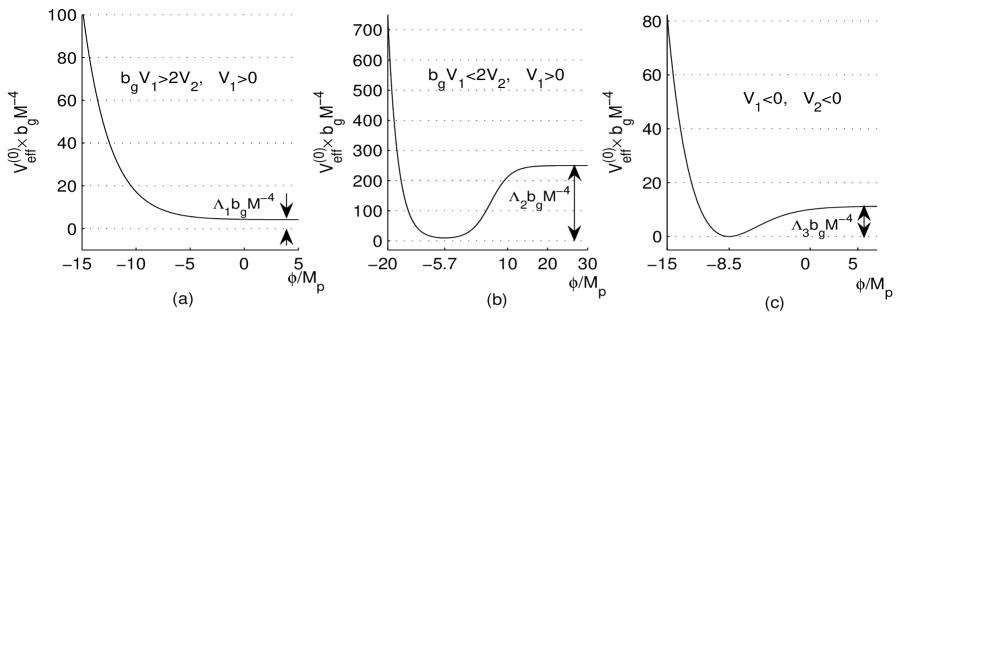
Figure 1: Three possible shapes of the effective potential $V_{eff}^{(0)}(\phi)$ in the models with $b_{g}V_{1}>V_{2}$:  Fig.(a)   $b_{g}V_{1}>2V_{2}$ (in the graph $V_{1}=10M^{4}$ and $V_{2}=4b_{g}M^{4}$);  Fig.(b)   $b_{g}V_{1}<2V_{2}$ (in the graph $V_{1}=10M^{4}$ and $V_{2}=9.9b_{g}M^{4}$). The value of $V_{eff}^{(0)}$ in the minimum $\phi_{min}=-5.7M_{p}$ is larger than zero;  Fig.(c)   $V_{1}<0$, $V_{2}<0$ (in the graph $V_{1}=-30M^{4}$ and $V_{2}=-50b_{g}M^{4}$). $V_{eff}^{(0)}(\phi_{min})=0$ in the minimum $\phi_{min}=-8.5M_{p}$ . In all the cases here as well as in all solutions presented in this paper we choose $\alpha=0.2$.

In the following three sections we consider three different dilaton-gravity cosmological models determined by different choice of the parameters $V_{1}$ and $V_{2}$ in the action with $\delta=0$: two models with $b_{g}V_{1}>V_{2}$ and $V_{1}>0$ and one model with $V_{1}<0$. The appropriate three possible shapes of the effective potential $V_{eff}^{(0)}(\phi)$ are presented in Fig.1. A special case with the fine tuned condition $b_{g}V_{1}=V_{2}$ is discussed in Appendix D where we show that equality of the couplings to measures $\Phi$ and $\sqrt{-g}$ in the action (equality $b_{g}V_{1}=V_{2}$ is one of the conditions for this to happen) gives rise to a symmetric form of the effective potential.

IV Cosmological Dynamics in the Model With $b_{g}V_{1}>2V_{2}$ and $\delta=0$:  Early Power Law Inflation Ending With Small $\Lambda$ Driven Expansion

In this model the effective potential (48) is a monotonically decreasing function of $\phi$ (see Fig.1a). As $M^{4}e^{-2\alpha\phi/M_{p}}\gg Max\left(V_{1},V_{2}/b_{g}\right)$, the effective potential (48) behaves as the exponential potential $V_{eff}^{(0)}\approx\frac{1}{4b_{g}}M^{4}e^{-2\alpha\phi/M_{p}}$. So, as $\phi\ll-M_{p}$ the model is able to describe a power law inflation of the early universepower-law if $\alpha<1/\sqrt{2}$. The latter condition will be assumed in all analytic solutions and qualitative discussions throughout the paper.

Applying this model to the cosmology of the late time universe and assuming that the scalar field $\phi\rightarrow\infty$ as $t\rightarrow\infty$, it is convenient to represent the effective potential (48) in the form

$$V_{eff}^{(0)}(\phi)=\Lambda_{1}+V_{q-l}(\phi).$$ (51)

where

$$\Lambda_{1}=\frac{V_{1}^{2}}{4(b_{g}V_{1}-V_{2})}$$ (52)

is the positive cosmological constant and

$$V^{(0)}_{q-l}(\phi)=\frac{(b_{g}V_{1}-2V_{2})V_{1}M^{4}e^{-2\alpha\phi/M_{p}}+(b_{g}V_{1}-V_{2})M^{8}e^{-4\alpha\phi/M_{p}}}{4(b_{g}V_{1}-V_{2})[b_{g}(V_{1}+M^{4}e^{-2\alpha\phi/M_{p}})-V_{2}]}.$$ (53)

We see that the evolution of the late time universe is governed both by the cosmological constant $\Lambda_{1}$ and by the quintessence-like potential $V^{(0)}_{q-l}(\phi)$.

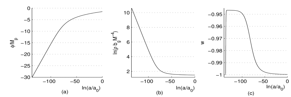
Figure 2: Typical dependence of the field $\phi$ (fig. (a)), the energy density $\rho$ (fig. (b)) and the equation-of-state $w$ (fig. (c)) upon $\ln(a/a_{0})$. Here and in all the graphs of this paper describing scale factor $a$ dependences, $a(t)$ is normalized such that at the end point of the described process $a(t_{end})=a_{0}$. The values of $V_{1}$ and $V_{2}$ are as in Fig.1a. The graphs correspond to the initial conditions $\phi_{in}=-50M_{p}$, $\dot{\phi}_{in}=-5M^{2}b_{g}^{-1/2}$. The early universe evolution is governed by the almost exponential potential (see Fig.1a) providing the power low inflation ($w\approx-0.95$ interval in fig.(c)). After transition to the late time universe the scalar $\phi$ increases with the rate typical for a quintessence scenario. Later on the cosmological constant $\Lambda_{1}$ becomes a dominated component of the dark energy that is displayed by the infinite region where $w\approx-1$ in fig.(c).

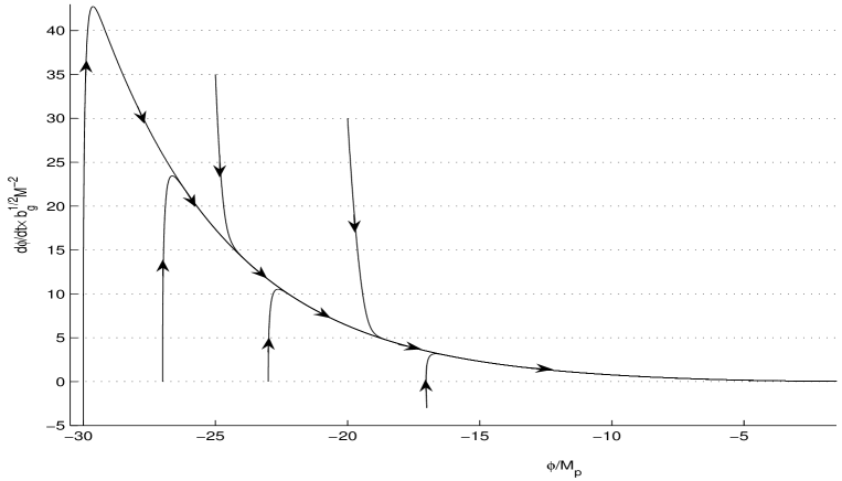
Figure 3: Phase portrait (plot of $\frac{d\phi}{dt}$ versus $\phi$) for the model with $b_{g}V_{1}>2V_{2}$. All trajectories approach the attractor which in its turn asymptotically (as $\phi\rightarrow\infty$) takes the form of the straight line $\dot{\phi}=0$.

The smallness of the observable cosmological constant, in this model given by $\Lambda_{1}$, is known as the new cosmological constant problemWeinberg2 . There are two ways to provide the observable order of magnitude of the present day vacuum energy density by an appropriate choice of the parameters of the theory.

(a) If $V_{2}<0$ then there is no need for $V_{1}$ and $V_{2}$ to be small: it is enough that $b_{g}V_{1}<|V_{2}|$ and $V_{1}/|V_{2}|\ll 1$. This possibility is a kind of seesaw mechanismG1 ,seesaw ). For instance, if $V_{1}$ is determined by the energy scale of electroweak symmetry breaking $V_{1}\sim(10^{3}GeV)^{4}$ and $V_{2}$ is determined by the Planck scale $V_{2}\sim(10^{18}GeV)^{4}$ then $\Lambda_{1}\sim(10^{-3}eV)^{4}$. The range of the possible scale of the dimensionless parameter $b_{g}$ remains very broad.

(b) If $V_{2}>0$ or alternatively $V_{2}<0$ and $b_{g}V_{1}>|V_{2}|$ then $\Lambda^{(0)}\approx\frac{V_{1}}{4b_{g}}$. Hence the second possibility is to choose the dimensionless parameter $b_{g}>0$ to be a huge number. In this case the order of magnitudes of $V_{1}$ and $V_{2}$ could be either as in the above case (a) or to be not too much different (or even of the same order). For example, if $V_{1}\sim(10^{3}GeV)^{4}$ then for getting $\Lambda_{1}\sim(10^{-3}eV)^{4}$ one should assume that $b_{g}\sim 10^{60}$. Note that $b_{g}$ is the ratio of the coupling constants of the scalar curvature to the measures $\sqrt{-g}$ and $\Phi$ in the fundamental action of the theory (9). Taking into account our assumption that the dimensionless parameters $b_{g}$, $b_{\phi}$, $k$ and $h_{i}$ $(i=N,E)$ are of the close order of magnitude, their huge values can be treated as a sort of a correspondence principle in the TMT. In fact, using the notations of the general form of the TMT action (1) in the case of the action (9), one can conclude that if these dimensionless parameters have the order of magnitude $\sim 10^{60}$ then the relation between the ”usual” (i.e. entering in the action with the usual measure $\sqrt{-g}$) Lagrangian $L_{2}$ and the new one $L_{1}$ (entering in the action with the new measure $\Phi$) is roughly speaking $L_{2}\sim 10^{60}L_{1}$. It seems to be very interesting that such a correspondence principle may be responsible for the extreme smallness of the cosmological constant.

Summing the above analysis we conclude that the effective potential (48) provides a possibility for a cosmological scenario which starts with a power law inflation and ends with a small cosmological constant $\Lambda_{1}$. It is very important that the effective potential (48) appears here as the result (in a certain range of parameters) of the TMT model undergoing the spontaneous breakdown of the global scale symmetry.

Results of numerical solutions for such type of scenario are presented in Figs.2 and 3 ($V_{1}=10M^{4}$, $V_{2}=4b_{g}M^{4}$) The early universe evolution is governed by the almost exponential potential (see Fig.1a) providing the power low inflation ($w\approx-0.95$ interval in fig.(c)) with the attractor behavior of the solutions, see Ref.Halliwell . After transition to the late time universe the scalar $\phi$ increases with the rate typical for a quintessence scenario. Later on the cosmological constant $\Lambda_{1}$ becomes a dominated component of the dark energy that is displayed by the infinite region where $w\approx-1$ in fig.(c). The phase portrait in Fig.3 shows that all the trajectories started with $|\phi|\gg M_{p}$ quickly approach the attractor which asymptotically (as $\phi\rightarrow\infty$) takes the form of the straight line $\dot{\phi}=0$. Qualitatively similar results are obtained also when $V_{1}$ is positive but $V_{2}$ is negative.

V Dilaton - Gravity model with $V_{1}>0$ and $V_{2}<b_{g}V_{1}<2V_{2}$

V.1 Cosmological Dynamics in the Case $\delta=0$

In this case the effective potential (48) has the minimum (see Fig.1b)

$$V^{(0)}_{eff}(\phi_{min})=\frac{V_{2}}{b_{g}^{2}}\qquad\text{at}\qquad\phi=\phi_{min}=-\frac{M_{p}}{2\alpha}\ln\left(\frac{2V_{2}-b_{g}V_{1}}{b_{g}}\right).$$ (54)

For the choice of the parameters as in Fig.1b, i.e. $V_{1}=10M^{4}$ and $V_{2}=9.9b_{g}M^{4}$, the minimum is located at $\phi_{min}=-5.7M_{p}$. The character of the phase portrait one can see in Fig.4.

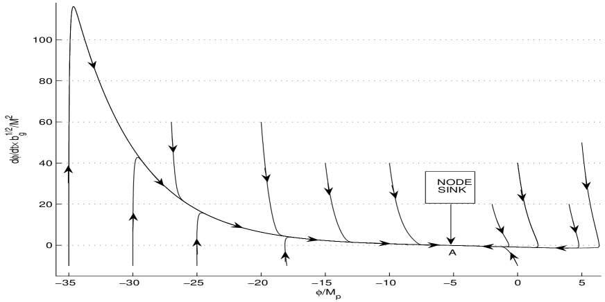
Figure 4: Typical behavior of the phase trajectories in the plane ($\phi$,$\frac{d\phi}{dt}$) for the model with $b_{g}V_{1}<2V_{2}$ and $V_{1}>0$ (the parameters are chosen here as in Fig.1b ). Trajectories started anywhere in the phase plane in a finite time end up at the same point $A(-5.7,0)$ which is a node sink. However there exist two attractors ending up at $A$, one from the left and other from the right in such a way that all phase trajectories starting with $|\phi|\gg M_{p}$ quickly approach these attractors.

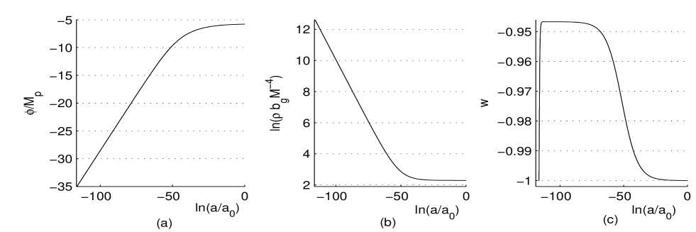
Figure 5: Cosmological dynamics in the model with $b_{g}V_{1}<2V_{2}$ and $V_{1}>0$: typical dependence of $\phi$ (Fig.(a)), the energy density $\rho$ (Fig.(b)) and the equation-of-state $w$ (Fig.(c)) upon $\ln(a/a_{0})$ where the scale factor $a(t)$ normalized as in Fig.2. The graphs correspond to the initial conditions $\phi_{in}=-35M_{p}$, $\dot{\phi}_{in}=-10b_{g}^{-1/2}M^{2}$. The early universe evolution is governed by an almost exponential potential (see Fig.1b) providing the power low inflation ($w\approx-0.95$ interval in Fig.(c)). After arriving the minimum of the potential at $\phi_{min}=-5.7M_{p}$ (see Fig.1b and the point $A(-5.7M_{p},0)$ of the phase plane in Fig.4) the scalar $\phi$ remains constant. At this stage the dynamics of the universe is governed by the constant energy density $\rho=V^{(0)}_{eff}(\phi_{min})$ (see the appropriate intervals $\rho=const$ in Fig.(b) and $w=-1$ in Fig.(c)).

For the early universe as $\phi\ll-M_{p}$, similar to what we have seen in the case of the monotonically decreasing potential in Sec.IV, the model implies the power low inflation. However, the phase portrait Fig.4 shows that now all solutions end up without oscillations at the minimum $\phi_{min}=-5.7M_{p}$ with $\frac{d\phi}{dt}=0$. In this final state of the scalar field $\phi$, the evolution of the universe is governed by the cosmological constant $V^{(0)}_{eff}(\phi_{min})$ determined by Eq.(54). For some details of the cosmological dynamics see Fig.5. The desirable smallness of $V^{(0)}_{eff}(\phi_{min})$ can be provided without fine tuning of the dimensionfull parameters by the way similar to what was done in item (b) of Sec.IV. The absence of appreciable oscillations in the minimum is explained by the following two reasons: a) the non-zero friction at the minimum determined by the cosmological constant $V^{(0)}_{eff}(\phi_{min})$; b) the shape of the potential near to minimum is too flat.

The described properties of the model are evident enough after the shape of the effective potential (20) in the Einstein frame is obtained in TMT. Nevertheless we have presented them here because this model is a particular (fine tuned) case of an appropriate model with $\delta\neq 0$ studied in the next subsection where we will demonstrate a possibility of states with $w<-1$ without phantom in the original action.

V.2 Dilaton - Gravity Cosmological Dynamics in the Case $\delta\neq 0$. Super-acceleration

We return now to the more general models of the scalar sector (see Sec.III) where the parameter $\delta$, defined by Eq.(30), is non zero. However we still ignore here the Higgs dynamics. The appropriate simplified version of the cosmological dynamics is of interest to us because it allows, without non relevant complications, to demonstrate the possibility of solutions for the late time universe with equation-of-state $w<-1$ (super-acceleration), which are favored by the present datasuperaccel ,Starobinsky

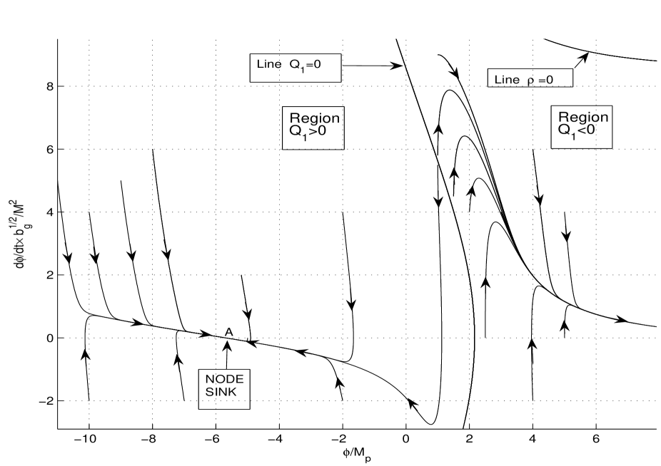
Figure 6: The phase portrait for the model with $\alpha=0.2$, $\delta=0.1$, $V_{1}=10M^{4}$ and $V_{2}=9.9b_{g}M^{4}$. The phase plane is divided up into two dynamically disconnected regions by the line $Q_{1}(\phi,\dot{\phi})=0$. To the left of this line $Q_{1}>0$ and to the right $Q_{1}<0$. The phase portrait in the left hand side, i.e. in the region $Q_{1}>0$, corresponds to processes similar to those of Sec.V.A. Trajectories in the right hand side of phase portrait, i.e. in the region $Q_{1}<0$, correspond to processes with super-accelerating expansion of the universe.

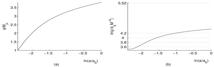
Figure 7: Scalar factor dependence of $\phi$ (Fig.(a)) and of the energy density $\rho$, defined by Eq.(35), (Fig(b)) in the regime of super-acceleration. Both graphs correspond to the initial conditions $\phi_{in}=M_{p}$, $\dot{\phi}_{in}=9M^{4}/\sqrt{b_{g}}$; $\rho$ increases approaching asymptotically $\Lambda_{2}=\frac{M^{4}}{b_{g}}e^{5.52}$.

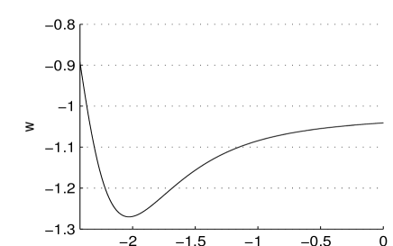
Figure 8: The scale factor dependence of the equation-of-state $w$ for the initial conditions $\phi_{in}=M_{p}$, $\dot{\phi}_{in}=9M^{4}/\sqrt{b_{g}}$.

So, we consider now the dynamics of the FRW cosmology described by Eqs.(45), (35), (37), (40)-(42) where $V_{1}$ and $V_{2}$ are constants and $\upsilon\equiv 0$. Adding the non zero $\delta$ to the parameter space enlarges significantly the number of classes of qualitatively different models. Among the new possibilities the most attractive one is the class of models giving rise to solutions for the late time universe with equation-of-state $w<-1$ without resorting to negative kinetic term in the fundamental action as in the phantom field modelsphantom .

Before choosing the appropriate parameters for numerical studies, let us start from the analysis of Eq.(37). The interesting feature of this equation is that for certain range of the parameters, each of the factors $Q_{i}(\phi,X)$  ($i=1,2,3$) can get to zero. Equation $Q_{i}(\phi,X)=0$ determines a line in the phase plane $(\phi,\dot{\phi})$. In terms of a mechanical interpretation of Eq.(37), the change of the sign of $Q_{1}$ can be treated as the change of the mass of ”the particle”. Therefore one can think of situation where ”the particle” climbs up in the potential with acceleration. It turns out that when the scalar field is behaving in this way, the flat FRW universe undergoes a super-acceleration.

There are a lot of sets of parameters providing this effect. For example we are demonstrating here this effect with the following set of the parameters of the original action(9): $\alpha=0.2$, $V_{1}=10M^{4}$ and $V_{2}=9.9b_{g}M^{4}$ used in Sec.IV but now we choose $\delta=0.1$. The results of the numerical solution are presented in Figs.6-8.

The phase plane, Fig.6, is divided into two dynamically disconnected regions by the line $Q_{1}(\phi,X)=0$. To the left of this line $Q_{1}>0$ and to the right $Q_{1}<0$. Comparing carefully the phase portrait in the region $Q_{1}>0$ with that in Fig.4 of the previous subsection, one can see an effect of $\delta\neq 0$ on the shape of phase trajectories. However the general structure of these two phase portraits is very similar. In particular, they have the same node sink $A(-5.7M_{p},0)$. At this point ”the force” equals zero since $Q_{3}|_{A}=0$. The value $\phi=-5.7M_{p}$ coincides with the position of the minimum of $V_{eff}^{(0)}(\phi)$ because in the limit $\dot{\phi}\rightarrow 0$ the role of the terms proportional to $\delta$ is negligible. Among trajectories converging to node $A$ there are also trajectories corresponding to a power low inflation of the early universe, which is just a generalization to the case $\delta\neq 0$ of the similar result discussed in the previous subsection.

On the right side of the phase plane Fig.6, i.e. in the region $Q_{1}<0$, all trajectories approach the attractor which in its turn asymptotically (as $\phi\rightarrow\infty$) takes the form of the straight line $\dot{\phi}=0$.

For a particular choice of the initial data $\phi_{in}=M_{p}$, $\dot{\phi}_{in}=9M^{4}/\sqrt{b_{g}}$, the features of the solution of the equations of motion are presented in Figs.7 and 8. The main features of the solution as we observe from the figures are the following: 1) $\phi$ slowly increases in time; 2) the energy density $\rho$ slowly increases approaching the constant $\Lambda=\Lambda_{2}$ defined by the same formula as in Eq.(52), see also Fig.1b; for the chosen parameters $\Lambda_{2}\approx\frac{M^{4}}{b_{g}}e^{5.52}$.  3) $w\equiv p/\rho$ is less than $-1$ and asymptotically approaches $-1$ from below.

Qualitative understanding of the fact that the energy density $\rho$ approaches $\Lambda_{2}$ during the super-accelerated expansion of the universe is based on the shape of the effective potential, Fig.1b, that would be in the model with $\delta=0$. However, the possibility of climbing up in the potential with acceleration can be understood only due to the effect of changing sign of $Q_{1}$, Eq.(40), which becomes possible in the model with $\delta\neq 0$. Due to such mechanism of the super-acceleration it becomes clear why qualitatively the same behavior one observes for all initial conditions $(\phi_{in},\dot{\phi}_{in})$ disposed in the region $Q_{1}<0$.

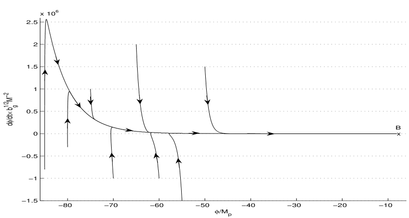
Figure 9: Phase portrait (plot of $\frac{d\phi}{dt}$ versus $\phi$) for the model with $V_{1}<0$ and $V_{2}<0$. All trajectories started with $|\phi|\gg M_{p}$ quickly approach the attractor long before entering the oscillatory regime. The region appropriate to the oscillatory regime is marked by point $B$. The oscillation spiral is not visible in Fig.11 because of the choice of the scale along the axis Y.

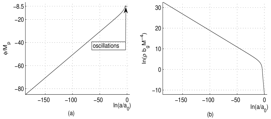
Figure 10: (a) In the model with $V_{1}<0$ the power law inflation ends with damped oscillations of $\phi$ around $\phi_{0}$ determined by Eq.(55). For the choice $V_{1}=-30M^{4}$ Eq.(55) gives $\phi_{0}=-8.5M_{p}$ . (b) The exit from the early inflation is accompanied with approaching zero of the energy density $\rho$. The graphs correspond to the evolution which starts from the initial values $\phi_{in}=-85M_{p}$, $\dot{\phi}_{in}=-8\cdot 10^{5}M^{2}/\sqrt{b_{g}}$.

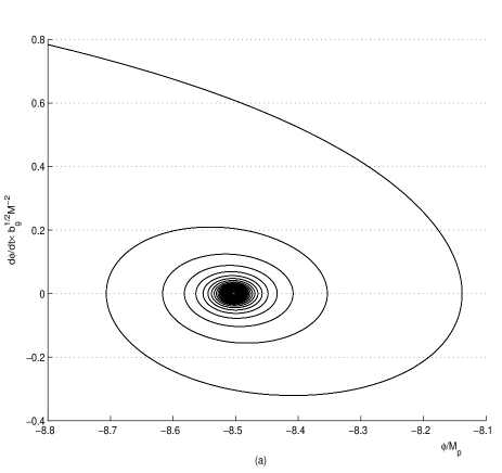
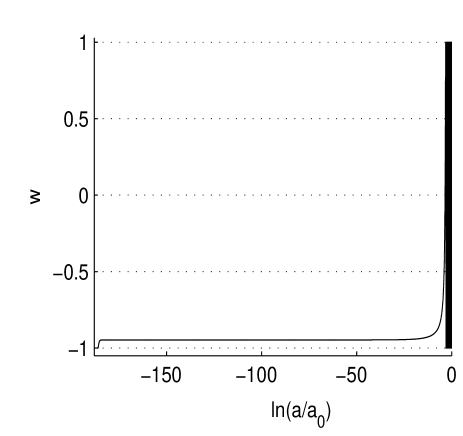
Figure 11: Fig.(a) zoom in on the oscillatory regime which marked by point B in Fig.9.   (b) Equation-of-state $w=p/\rho$ as function of the scale factor for the parameters and initial conditions as in Fig.10. Most of the time the expansion of the universe is a power law inflation with almost constant $w\approx-0.95$; $w$ oscillates between $-1$ and $1$ at the exit from inflation stage, i.e. as $\phi\rightarrow\phi_{0}$ and $\rho\rightarrow 0$

VI Dilaton - Gravity Cosmological Dynamics in the Model with $V_{1}<0$ and $V_{2}<0$. The Old Cosmological Constant Problem and Non Applicability of the Weinberg Theorem

The most remarkable features of the effective potential (48) is that it is proportional to the square of $V_{1}+M^{4}e^{-2\alpha\phi/M_{p}}$. Due to this, as $V_{1}<0$ and $V_{2}<0$, the effective potential has a minimum where it equals zero automatically, without any further tuning of the parameters $V_{1}$ and $V_{2}$ (see also Fig.1c). This occurs in the process of evolution of the field $\phi$ at the value of $\phi=\phi_{0}$ where

$$V_{1}+M^{4}e^{-2\alpha\phi_{0}/M_{p}}=0.$$ (55)

This means that the universe evolves into the state with zero cosmological constant without tuning parameters of the model.

If such type of the structure for the scalar field potential in a usual (non TMT) model would be chosen ”by hand” it would be a sort of fine tuning. But in our TMT model it is not the starting point, it is rather a result obtained in the Einstein frame of TMT models with spontaneously broken global scale symmetry including the shift symmetry $\phi\rightarrow\phi+const$. Later on we will see the same effect in more general models including also the Higgs field as well as in models with $\delta\neq 0$. Note that the assumption of scale invariance is not necessary for the effect of appearance of the perfect square in the effective potential in the Einstein frame and therefore for the described mechanism of disappearance of the cosmological constant, see Refs.GK2 -G1 and Appendix E.

On the first glance this effect contradicts the no-go Weinberg theoremWeinberg1 which states that there cannot exist a field theory model where the cosmological constant is zero without fine tuning. Recall that one of the basic assumptions of this no-go theorem is that all fields in the vacuum must be constant. However, this is not the case in TMT. In fact, in the vacuum determined by Eq.(55) the scalar field $\zeta\equiv\frac{\Phi}{\sqrt{-g}}$ is non zero, see Eq.(46). The latter is possible only if all the $\varphi_{a}$ ($a=1,2,3,4$) fields (in the definition of $\Phi$ by means of Eq.(2)) or the 3-index potential $A_{\alpha\beta\gamma}$ (when using the definition of $\Phi$ by means of Eq.(3)) have non vanishing space-time gradients. Moreover, exactly in the vacuum $\phi=\phi_{0}$ the scalar field $\zeta$ has a singularity. However, in the conformal Einstein frame all physical quantities are well defined and this singularity manifests itself only in the vanishing of the vacuum energy density. We conclude therefore that the Weinberg theoremWeinberg1 is not applicable in the context of the TMT models studied here. In fact, the possibility of such type of situation was suspected by S. Weinberg in the footnote 8 of his reviewWeinberg1 where he pointed out that when using a 3-index potential with non constant vacuum expectation value, his theorem does not apply.

The results of numerical solutions are evident enough, but we want to present them here because they will be useful for comparison with the results of the next section. For the potential of Fig.1c (where we have chosen $V_{1}=-30M^{4}$ and $V_{2}=-50b_{g}M^{4}$) the results of numerical solutions are presented in figures 9,10,11.

VII Higgs-Inflaton Symbiosis: Inflation, Exit From Inflation And New Cosmological Mechanism for gauge symmetry breaking

VII.1 General Discussion

Turning now to the general case of the scalar sector, Sec.III, where both dilaton and Higgs dynamics are taken into account, we have to make some nontrivial choices for the Higgs pre-potentials $V_{1}(\upsilon)$ and $V_{2}(\upsilon)$. We will see that for achieving a gauge symmetry breakdown there is no need for tachyonic mass terms in $V_{1}(\upsilon)$ and $V_{2}(\upsilon)$ and even for selfinteraction terms. We make the following simplest choice

$$V_{1}=V_{1}^{(0)}+\mu_{1}^{2}\upsilon^{2};\qquad V_{2}=V_{2}^{(0)}+\mu_{2}^{2}\upsilon^{2}$$ (56)

assuming

$$\mu_{1}^{2}>0,\qquad\mu_{2}^{2}>0\qquad\text{and}\qquad V_{1}^{(0)}<0,\qquad V_{2}^{(0)}<0$$ (57)

In order to understand qualitatively what is the mechanism of the gauge symmetry breaking it is useful to start from the model with $\delta=0$. Then from Eqs.(20) and (33) we get for $\delta=0$

$$V_{eff}(\phi,\upsilon)=\frac{[V_{1}^{(0)}+\mu_{1}^{2}\upsilon^{2}+M^{4}e^{-2\alpha\phi/M_{p}}]^{2}}{4\left[\left(b_{g}V_{1}^{(0)}-V_{2}^{(0)}\right)+\left(b_{g}\mu_{1}^{2}-\mu_{2}^{2}\right)\upsilon^{2}+b_{g}M^{4}e^{-2\alpha\phi/M_{p}}\right]}$$ (58)

Even in this simple model the effective potential of the scalar sector contains a very non-trivial coupling between dilaton, playing the role of inflaton, and Higgs fields. It is easy to see that this coupling disappears in the limit $\phi\ll-M_{p}$ corresponding to the very early universe:

$$V_{eff}(\phi,\upsilon)|_{early\,universe}\approx\frac{1}{4b_{g}}M^{4}e^{-2\alpha\phi/M_{p}}+\frac{1}{4b_{g}^{2}}(b_{g}\mu_{1}^{2}+\mu_{2}^{2})\upsilon^{2}+const.$$ (59)

Therefore, in the very early universe, the minimization of $V_{eff}$ is achieved at $\upsilon=0$ which means that the Higgs field is in an unbroken symmetry phase without resorting to high temperature effects. So, in the very early cosmological epoch, we have $V_{1}=V_{1}^{(0)}<0$,   $V_{2}=V_{2}^{(0)}<0$ and $V_{eff}\approx\frac{1}{4b_{g}}M^{4}e^{-2\alpha\phi/M_{p}}$ and therefore one can use the results of Sec.VI in what it concerns to the early inflationary epoch. It turns out, however, that this preliminary analysis is unable to give a complete scenario of the early inflationary epoch, see the next two subsections.

If we want $V_{eff}(\phi,\upsilon)$ to be positive definite and the symmetry broken state to be the absolute minimum we have to assume in addition that

$$b_{g}V_{1}^{(0)}\geq V_{2}^{(0)},\qquad b_{g}\mu_{1}^{2}\geq\mu_{2}^{2}$$ (60)

This will be our choice.

It is interesting that in the particular case $b_{g}\mu_{1}^{2}=\mu_{2}^{2}$ the effective potential (58) can be written in the form of the Ginzburg-Landau type potential for the Higgs field $\upsilon$

$$V_{eff}(\phi,\upsilon)|_{b_{g}\mu_{1}^{2}=\mu_{2}^{2}}=\lambda(\phi)[\upsilon^{2}-\sigma^{2}(\phi)]^{2},$$ (61)

where the coupling ”constant” $\lambda$ and the mass parameter $\sigma$ are the following functions of $\phi$:

$$\lambda(\phi)=\mu_{1}^{4}\left[4\left(b_{g}V_{1}^{(0)}-V_{2}^{(0)}+b_{g}M^{4}e^{-2\alpha\phi/M_{p}}\right)\right]^{-1};\qquad\sigma^{2}(\phi)=\mu_{1}^{-2}\left(|V_{1}^{(0)}|-M^{4}e^{-2\alpha\phi/M_{p}}\right).$$ (62)

If the Higgs field were to remain in the unbroken phase $\upsilon=0$, then according to Sec.VI, the power law inflation would be ended with oscillations of the $\phi$-field accompanied with approaching zero of the energy density. However decreasing $M^{4}e^{-2\alpha\phi/M_{p}}$ causes that $\partial^{2}V_{eff}/\partial\upsilon^{2}$ gets to be zero. The continuation of this process changes the shape of the Higgs dependence of the effective scalar sector potential such that $\upsilon=0$ turns into local maximum and a nonzero $\upsilon=<\upsilon>\neq 0$ appears as the true minimum of the effective scalar field potential (58) in the $\upsilon$ direction. This happens as $<\upsilon>^{2}$ and $\phi=\phi_{0}$ satisfy the equation of the following curve

$$V_{1}^{(0)}+\mu_{1}^{2}<\upsilon>^{2}+M^{4}e^{-2\alpha\phi_{0}/M_{p}}=0,$$ (63)

which at the same time, is also the condition for the minimum in the $\phi$ direction (see also Eqs.(37)-(43) as $\delta=0$). The remarkable feature of the effective potential (58) is that in this minimum it equals zero without fine tuning of the parameters of the action. This vacuum with zero cosmological constant is degenerate. Notice however that this degeneracy has no relation to any symmetry of the action.

This degeneracy is a particular manifestation of the well known more general feature of the systems with two interacting scalar fields: if both of them are dynamically important then as noted in Ref.Liddle , there is no attractor behavior giving a unique route into the potential minimum, as it happens in the single field case. However, numerical and analytic solutions show that in spite of this general statement, for the system under consideration, in a broad enough range of the parameters $\alpha$, $\delta$, $V_{1}^{(0)}<0$,   $V_{2}^{(0)}<0$,   $\mu_{1}^{2}>0$ and $\mu_{2}^{2}>0$, both fields, i.e $\phi$ and $\upsilon$, are dynamically important but there exists an attractor behavior. As a result of this there is only one very short segment in the line (63) where all the phase trajectories end in the process of the cosmological evolution. In other words, the magnitudes of $<\upsilon>^{2}$ and $\phi_{0}$ are determined by the values of the parameters of the model but dependence upon the initial values $\phi_{in}$,   $\dot{\phi}_{in}$,   $\upsilon_{in}$ and $\dot{\upsilon}_{in}$ is extremely weak.

For the study of numerical and analytical solutions as well as for detailed qualitative analysis of all the stages of the scalar sector evolution during the cosmological expansion it will be sometimes convenient to work with the equations of motion (37)-(43) written in terms of dimensionless parameters and variables. Then Eqs.(37) and (38) take the following form (here we restrict ourselves with the choice $\delta=0$)

$$\frac{d^{2}\varphi}{d\tau^{2}}+\sqrt{3\epsilon}\frac{d\varphi}{d\tau}-\alpha e^{-2\alpha\varphi}\frac{\left(\tilde{V}_{1}(\tilde{\upsilon})+e^{-2\alpha\varphi}\right)\left(\tilde{V}_{1}(\tilde{\upsilon})-2\tilde{V}_{2}(\tilde{\upsilon})+e^{-2\alpha\varphi}\right)}{2\left(\tilde{V}_{1}(\tilde{\upsilon})-\tilde{V}_{2}(\tilde{\upsilon})+e^{-2\alpha\varphi}\right)^{2}}=0$$ (64)

$$\frac{d^{2}\tilde{\upsilon}}{d\tau^{2}}+\sqrt{3\epsilon}\frac{d\tilde{\upsilon}}{d\tau}$$ (65)

$$+ \left(\frac{M_{p}}{M}\right)^{2}\frac{\tilde{V}_{1}(\tilde{\upsilon})+e^{-2\alpha\varphi}}{2\left(\tilde{V}_{1}(\tilde{\upsilon})-\tilde{V}_{2}(\tilde{\upsilon})+e^{-2\alpha\varphi}\right)^{2}}\left[\tilde{\mu}^{2}_{1}\left(\tilde{V}_{1}(\tilde{\upsilon})-2\tilde{V}_{2}(\tilde{\upsilon})+e^{-2\alpha\varphi}\right)+\tilde{\mu}^{2}_{2}\left(\tilde{V}_{1}(\tilde{\upsilon})+e^{-2\alpha\varphi}\right)\right]\tilde{\upsilon}=0$$

where Eq.(45) and the following dimesionless parameters and variables have been used

$$\tilde{V}_{1}^{(0)}=\frac{V_{1}^{(0)}}{M^{4}};\quad\tilde{V}_{2}^{(0)}=\frac{V_{2}^{(0)}}{b_{g}M^{4}};\quad\tilde{\mu}_{1}^{2}=\frac{\mu_{1}^{2}}{M^{2}};\quad\tilde{\mu}_{2}^{2}=\frac{\mu_{2}^{2}}{b_{g}M^{2}};\quad$$

$$\tau=\frac{M^{2}}{M_{p}\sqrt{b_{g}}}t;\qquad\varphi=\frac{\phi}{M_{p}};\quad\tilde{\upsilon}=\frac{\upsilon}{M};\quad\tilde{V}_{i}(\tilde{\upsilon})=\tilde{V}_{i}^{(0)}+\tilde{\mu}_{i}^{2}\tilde{\upsilon}^{2},\quad i=1,2$$ (66)

and

$$\epsilon=\frac{b_{g}}{M^{4}}\rho=\tilde{X}+\frac{1}{2}\left(\frac{M}{M_{p}}\right)^{2}\left(\frac{d\tilde{\upsilon}}{d\tau}\right)^{2}+V_{eff}^{(0)}(\varphi,\tilde{\upsilon}),$$ (67)

where

$$V_{eff}(\varphi,\tilde{\upsilon})=\frac{\left(\tilde{V}_{1}^{(0)}+\tilde{\mu}_{1}^{2}\tilde{\upsilon}^{2}+e^{-2\alpha\varphi}\right)^{2}}{4\left[\tilde{V}_{1}^{(0)}-\tilde{V}_{2}^{(0)}+\left(\tilde{\mu}_{1}^{2}-\tilde{\mu}_{2}^{2}\right)\tilde{\upsilon}^{2}+e^{-2\alpha\varphi}\right]},$$ (68)

$$\tilde{X}=\frac{1}{2}\left(\frac{d\varphi}{d\tau}\right)^{2}=\frac{b_{g}}{M^{4}}X;\quad\left(\frac{d\tilde{\upsilon}}{d\tau}\right)^{2}=\frac{b_{g}M_{p}^{2}}{M^{6}}\left(\frac{d\upsilon}{dt}\right)^{2}$$ (69)

and $X$ is defined by Eq.(34).

In terms of the dimensionless quantities, the equation for the manifold of the true vacuum (63) takes the form

$$e^{-2\alpha\varphi_{0}}=|\tilde{V}_{1}^{(0)}|-\tilde{\mu}_{1}^{2}<\tilde{\upsilon}>^{2}.$$ (70)

It follows from the positivity of the r.h.s. of Eq.(70) that

$$<\tilde{\upsilon}>^{2}\,<\,\frac{|\tilde{V}_{1}^{(0)}|}{\tilde{\mu}_{1}^{2}}.$$ (71)

Vacuum expectation value $<\tilde{\upsilon}>$ is indeed a minimum of the effective potential (68) in the $\tilde{\upsilon}$ direction if the frequency squared of the $\tilde{\upsilon}$ oscillations around the vacuum manifold (70) is positive:

$$\omega^{2}(<\tilde{\upsilon}>^{2})\equiv\frac{\partial^{2}V_{eff}}{\partial\tilde{\upsilon}^{2}}|_{vacuum\,manifold}=\frac{2\tilde{\mu}_{1}^{2}\tilde{\mu}_{2}^{2}<\tilde{\upsilon}>^{2}}{|\tilde{V}_{2}^{(0)}|-\tilde{\mu}_{2}^{2}<\tilde{\upsilon}>^{2}}\,>\,0,$$ (72)

We conclude from (71) and (72) that the vacuum expectation value $<\tilde{\upsilon}>^{2}$ has to satisfy the upper bound

$$<\tilde{\upsilon}>^{2}\quad<\quad Min\left(\frac{|\tilde{V}_{1}^{(0)}|}{\tilde{\mu}_{1}^{2}},\quad\frac{|\tilde{V}_{2}^{(0)}|}{\tilde{\mu}_{2}^{2}}\right)$$ (73)

VII.2 Numerical Solutions and Their Physical Meaning

We are presenting here the results of the numerical solutions for equations of motion in the model with the following set of the parameters:

$$\alpha=0.2,\quad M=10^{-2}M_{p}\sim 10^{16}GeV,\quad V_{1}^{(0)}=-30M^{4},\,V_{2}^{(0)}=-50b_{g}M^{4},\,\mu_{1}^{2}=20M^{2},\,\mu_{2}^{2}=10M^{2}.$$ (74)

The choice of the GUT scale for the integration constant $M$ seems to us to be the most natural. But restricting with a single Higgs field we proceed actually in a toy model.

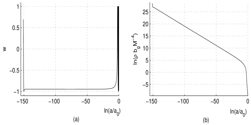
Figure 12: Behavior of the equation-of-state $w$, Fig.(a), and the energy density $\rho$, Fig.(b), as functions of $ln(a/a_{0})$, typical for all sets of the initial conditions, Eqs(75). (76). During a short time at the beginning $w>0$ because of the big value of the inflaton kinetic energy. The graph of $w$ exhibit that most of the time of the evolution the equation-of-state is close to the constant $w\approx-0.95$. This power low inflation ends (i.e. $w\approx-\frac{1}{3}$. ) as $\ln a/a_{0}\approx-3$. After the end of inflation the energy density $\rho$ quickly approaches zero. The equation-of-state at this period is not well defined due to oscillations of the Higgs field.

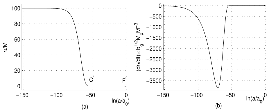
Figure 13: The scale factor dependence of the Higgs field $\upsilon$, Fig.(a), and its time derivative, Fig.(b), typical for all the initial conditions, Eq.(75); here the solution for the set (4) of the initial conditions is displayed. During the first stage of the inflation (the GSB inflation, see the main text) $\upsilon$ varies very slowly from its initial value $\upsilon_{in}$. After the point $C^{\prime}$, i.e. during the GSR inflation, $\upsilon$ is very close to zero (oscillates around $\upsilon=0$). After the point $F^{\prime}$ the Higgs-inflaton system fulfils a transition to ”zero cosmological constant and broken gauge symmetry” phase where the Higgs field oscillates with decaying amplitude around the vacuum manifold (63).

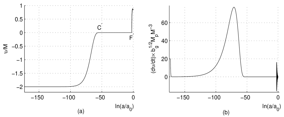
Figure 14: The same as in Fig.13 for the set (2) of the initial conditions.

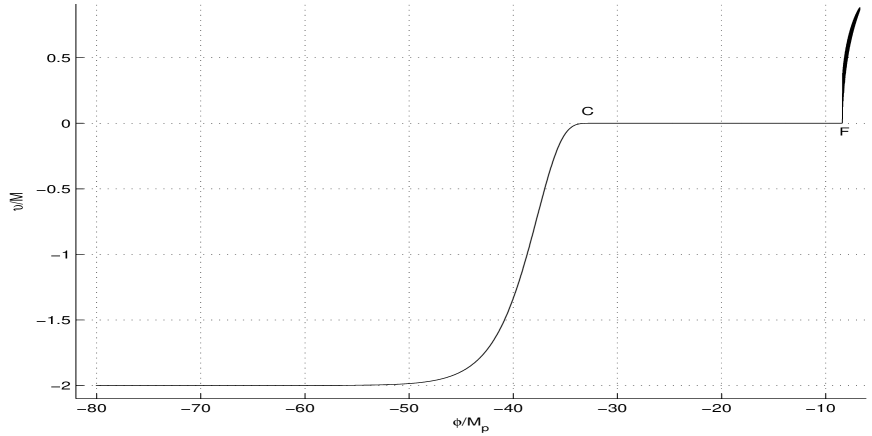
Figure 15: Projection on the plane $(\phi,\upsilon)$ of the 4-dimensional phase trajectory corresponding to the solution for the set (2) of the initial conditions. The function $\upsilon(\phi)$ starts from $\upsilon=-2M$ and changes very slowly during the GSB inflation. After transition to the GSR inflation (after the point $C$) the phase trajectory approaches the attractor ($\dot{\phi}=0$, $\upsilon=0$, $\dot{\upsilon}=0$) via oscillations of $\upsilon$ around $\upsilon=0$, see below. The last phase transition during of which the Higgs-inflaton system evolves (with damping oscillations of $\upsilon$) along the vacuum manifold (70) is presented by the ”horn” after the point $F$. The middle line of the horn is in fact the vacuum manifold (70).

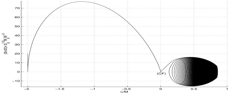
Figure 16: Typical behavior of the projections of the 4-dimensional phase trajectories on the plane $(\upsilon,\dot{\upsilon})$; here the solution for the set (2) of the initial conditions has been used. The vertical line $\upsilon\approx-2$ exhibits the stage of the GSB inflation. The large curve corresponds to the transition from the GSB inflation to the GSR inflation. The point labeled by $(CF)$ is the projection of the interval $CF$ in Fig.15 on the $(\upsilon,\dot{\upsilon})$ plane. After $(CF)$ the Higgs field $\upsilon$ evolves via oscillations from the practically zero value to the gauge symmetry broken phase with the vacuum expectation value $<\upsilon>$ which in the graph is about 0.84M.

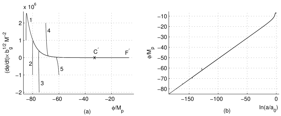
Figure 17: Projections on the phase plane $(\phi,\dot{\phi})$ of five 4-dimensional phase trajectories corresponding to five sets of the initial conditions (75), Fig.(a). Similar to Fig.11 in Sec.VI, the trajectories exhibit quick approach to the attractor $\dot{\phi}=0$. Point $C^{\prime}$ corresponds to the beginning of the second stage of inflation (the GSR inflation) which succeeds the first stage of inflation (the GSB inflation). The phase trajectories become very close to the attractor $\dot{\phi}=0$ long before the point $C^{\prime}$. Point $F^{\prime}$ corresponds to the start of the phase transition to the ”zero cosmological constant and broken gauge symmetry” phase. Fig.(b) includes the scale factor dependence of the inflaton for five sets of the initial conditions (75).

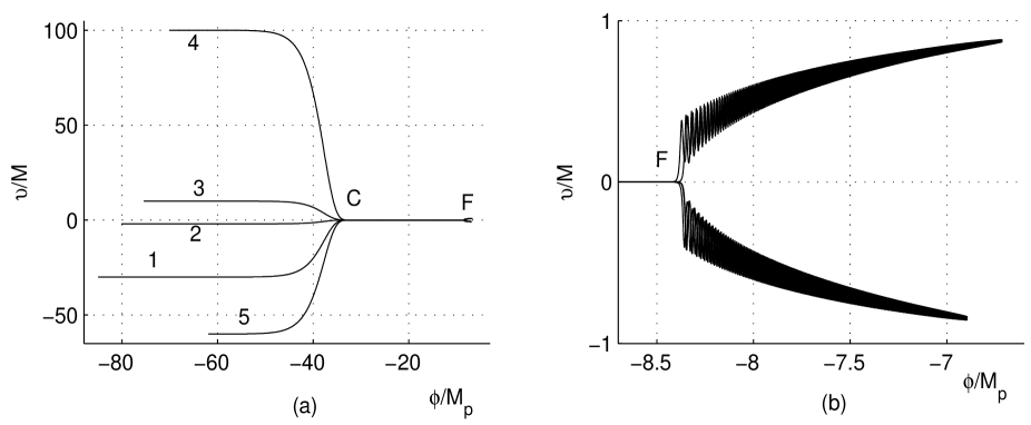
Figure 18: Projections on the phase plane $(\phi,\upsilon)$ of five 4-dimensional phase trajectories corresponding to five sets of the initial conditions (75). A surprising feature of the dynamics consists in the observed fact that independently of the initial conditions, all the phase trajectories achieve the line $\upsilon=0$ at the same value of $\phi$, i.e. the point C is the common point for all phase trajectories. Moreover, it turns out that points F for different phase trajectories are also very close to each other: see Fig.(b) which zooms in on the the behavior of the five phase trajectories after the point F. Two horns show that the five phase trajectories are divided into two directions giving $<\upsilon>$ of both signs (recall that this sign has no physical meaning). The final values of $|<\upsilon>|$ corresponding to different conditions are very close (see however the appropriate discussion in the main text).

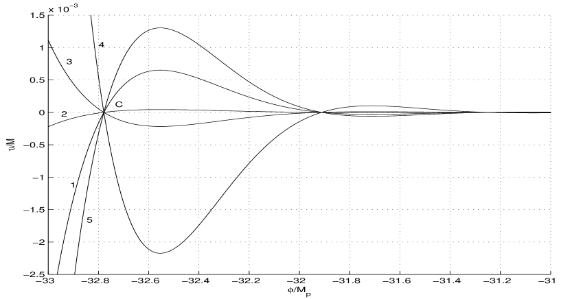
Figure 19: This figure zooms in on the behavior of the five phase trajectories (corresponding to the five sets of the initial conditions (75)) near and after the point $C$ in Fig.18a. Solutions $\upsilon(\phi)$ exhibit the behavior typical for Bessel functions. This feature as well as the reason of an observed synchronism will be explained in Sec.VIIC.

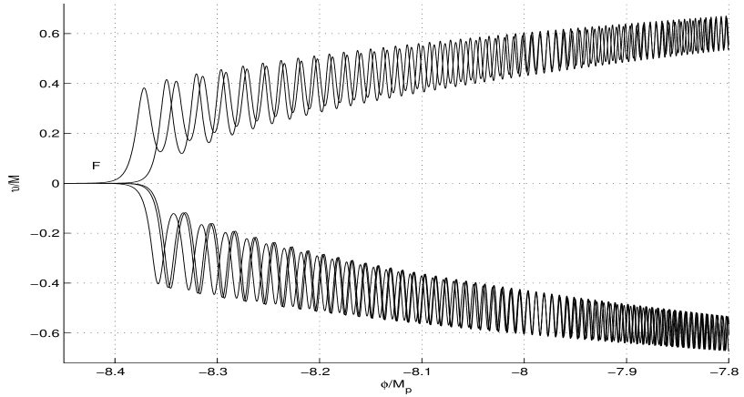
Figure 20: This figure zooms in on two horns in Fig.18b. One can see that amplitudes of the oscillations of $\upsilon$ around the line of the vacuum manifold quickly become practically equal for solutions with different initial conditions. Frequency of oscillations increases with $\upsilon$, see Eq.(72).

In the main part of this subsection we choose $\delta=0$. But afterwards, at the end of the subsection, we show that the main results holds even if $\delta\neq 0$.

To explore the effect of the initial conditions ($\phi_{in},\dot{\phi}_{in},\upsilon_{in},\dot{\upsilon}_{in})$ on the evolution of the inflaton $\phi$ and the Higgs field $\upsilon$ we have solved the equations for six sets of the initial conditions. Figures 12-20 demonstrate the results for following five sets of them:

$$(1) \varphi_{in}=-85,\quad\tilde{\upsilon}_{in}=-30,\quad\frac{d\varphi}{d\tau}|_{in}=10^{6},\quad\frac{d\tilde{\upsilon}}{d\tau}|_{in}=-20;$$ (75)

$$(2) \varphi_{in}=-80,\quad\tilde{\upsilon}_{in}=-2,\quad\frac{d\varphi}{d\tau}|_{in}=-10^{6},\quad\frac{d\tilde{\upsilon}}{d\tau}|_{in}=20;$$

$$(3) \varphi_{in}=-75,\quad\tilde{\upsilon}_{in}=10,\quad\frac{d\varphi}{d\tau}|_{in}=-2\cdot 10^{6},\quad\frac{d\tilde{\upsilon}}{d\tau}|_{in}=50;$$

$$(4) \varphi_{in}=-70,\quad\tilde{\upsilon}_{in}=100,\quad\frac{d\varphi}{d\tau}|_{in}=2\cdot 10^{6},\quad\frac{d\tilde{\upsilon}}{d\tau}|_{in}=-30;$$

$$(5) \varphi_{in}=-60,\quad\tilde{\upsilon}_{in}=-60,\quad\frac{d\varphi}{d\tau}|_{in}=-10^{6},\quad\frac{d\tilde{\upsilon}}{d\tau}|_{in}=40.$$

The results for the sixth set of the initial conditions

$$(6) \varphi_{in}=-70,\quad\tilde{\upsilon}_{in}=-0.01,\quad\frac{d\varphi}{d\tau}|_{in}=-2\cdot 10^{6},\quad\frac{d\tilde{\upsilon}}{d\tau}|_{in}=-5$$ (76)

are shortly presented separately in Fig.21. This is done just for technical reason because $\tilde{\upsilon}_{in}$ is too small.

So we are exploring the numerical solutions in the broad enough range of the initial values of the Higgs field $\upsilon$

$$10^{14}GeV\leq\upsilon_{in}\leq 10^{18}GeV$$ (77)

while according to (73) the true vacuum expectation value $<\tilde{\upsilon}>$ is bounded by

$$|<\upsilon>|<1.22\cdot 10^{16}GeV$$ (78)

Fig.12 shows the behavior of the energy density and equation-of-state typical for all the initial conditions we have checked. For the set of the initial conditions (4), Eq.(75), Fig.13 shows the evolution of $\upsilon$ and $\dot{\upsilon}$ as functions of the scale factor. Using as a pattern the set of the initial conditions (2), Eq.(75), in Figs.14-16 we demonstrate the main features of the cosmological evolution of the Higgs-inflaton system. Figs.17-20 allow to show that dependence of these features upon the initial conditions is very weak. In Fig.21 we show that the interval of the initial conditions may be significantly expanded without altering the latter conclusion. In Fig.22 we present the scale factor dependence of the Higgs field for four sets of initial conditions different from those in Eqs.(75) and (76). Figs.23 and 24 show two additional facts: 1) the inflaton also oscillates during the transition to the symmetry broken phase, although its amplitudes are much less that those of the Higgs field; 2) exact detection of the finishing point $(\phi_{0},<\upsilon>)$ of the pure classical transition to the symmetry broken phase is problematic. Finally, in Figs.25-26 we show that the effect of the parameter $\delta$ on the the main features of the cosmological evolution of the Higgs-inflaton system, including the final gauge symmetry broken phase, is also very weak.

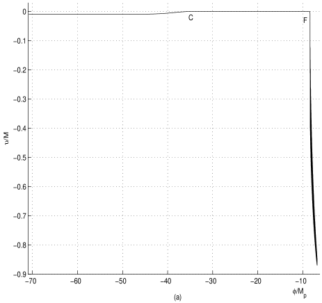
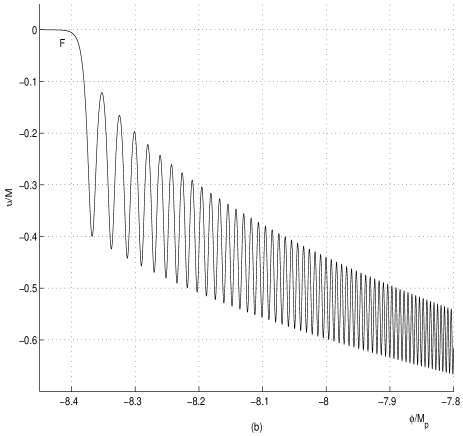
Figure 21: The effects displayed for the sets of the initial conditions (75) hold for larger range of the initial values of $\upsilon$. Here for example we present the solution for the set (76) of the initial conditions where $\tilde{\upsilon}_{in}=-0.01$. The locations of points C and F are the same as in Fig.18b; amplitudes of the oscillations of $\upsilon$ around the line of the vacuum manifold are very close to those in Fig.20. The final value of $|<\upsilon>|$ is very close to those we have observed for the sets of the initial conditions (75).

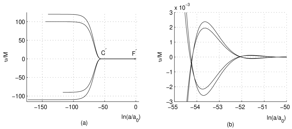
Figure 22: Fig.(a) Scale factor dependence of the Higgs field for four different initial conditions with $\tilde{\upsilon}_{in}\sim 10^{2}$ exhibits that the GSR inflation starts about 50 e-folding before the end of inflation. Fig.(b) zooms in on the interval near and after the point $C^{\prime}$.

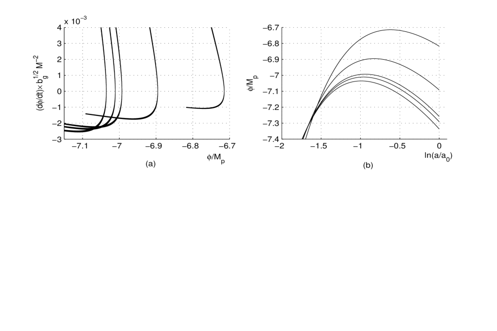
Figure 23: Fig.(a) zooms in on the behavior of the five phase trajectories in Fig.17a in the region after the point $F^{\prime}$: evolving together with $\upsilon$ along the vacuum manifold (70), $\phi$ performs a recoil with change of the sign of $d\phi/dt$ from positive to negative as the period average of $d\phi/dt$ gets to zero. Fig.(b) shows details of the scalar factor dependence of $\phi$ at the end of the process displayed in Fig.17b (i.e. during the transition to the gauge symmetry broken phase) for the same five sets of the initial conditions (75).

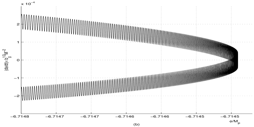
Figure 24: Figure zooms in on one of the trajectories in Fig.23a (namely for the trajectory with the set of the initial conditions (2) in (75)) near to the region where the period average of $d\phi/dt$ gets to zero.

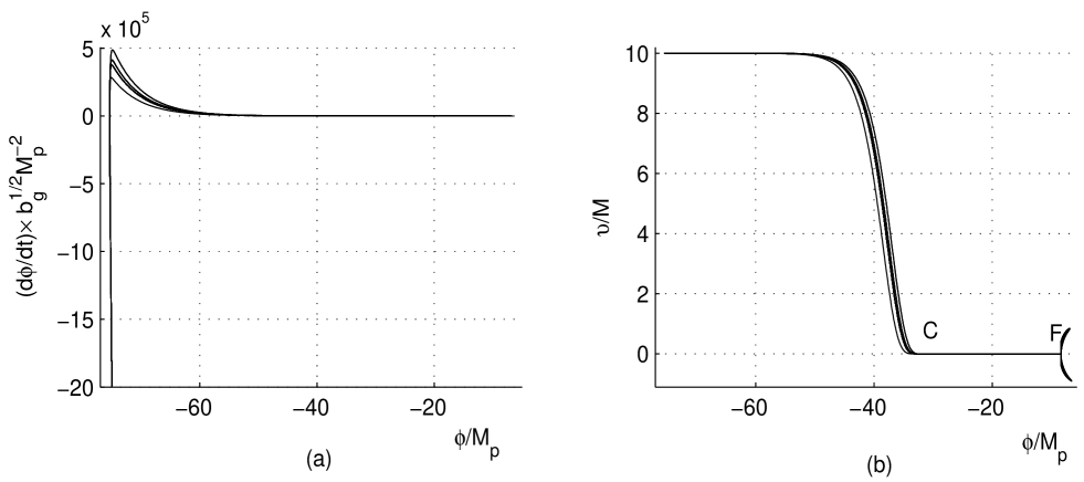
Figure 25: The effect of the parameter $\delta$, Eq.(30), on the dynamics of the Higgs-inflaton symbiosis. Four graphs in Figs. (a) and (b) correspond to the solutions with the fixed initial conditions (3) in Eq.(75) while for the parameter $\delta$ we have chosen the values $\delta=0$,   $\delta=0.2$,   $\delta=0.5$,   $\delta=0.7$.

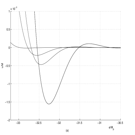
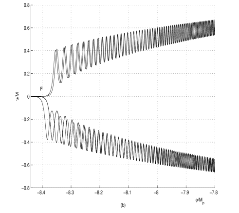
Figure 26: Figures zoom in on the graphs in Fig.25b near and after C, and near and after F. Although location of the point C is $\delta$-dependent (as we see in Fig.(a)), the oscillatory regime of the approach of the Higgs field to the final value of $<\upsilon>$ is practically independent of $\delta$.

Fig.12b demonstrates the fact discussed in detail after Eq.(63)), that transition to the gauge symmetry broken phase at the same time is the transition to the state with zero vacuum energy density.

Fig.12a demonstrates that most of the time of the evolution the equation-of-state is close to the constant $w\approx-0.945$. This corresponds to a power low inflation which ends (i.e. $w\approx-\frac{1}{3}$) as $\ln a/a_{0}\approx-3$ and $\phi/M_{p}\approx-10$ (the latter one can see analyzing Figs.12b and 17b). The qualitative explanation of this effect is evident enough. In fact, with our choice of the order of magnitudes of the parameters and initial conditions, contributions of $e^{-2\alpha\varphi}$ strongly dominate over all the terms both in numerator and denominator of the potential (68) as $\varphi\leq-15$, i.e in terms of the dimensionless quantities(66):

$$e^{-2\alpha\varphi}\gg Max\left[\left(\frac{M}{M_{p}}\cdot\frac{d\tilde{\upsilon}}{d\tau}\right)^{2},\tilde{V}_{1}^{(0)},\tilde{V}_{2}^{(0)},\tilde{\mu}_{1}^{2}\tilde{\upsilon}^{2},\tilde{\mu}_{2}^{2}\tilde{\upsilon}^{2}\right]$$ (79)

Therefore for $\varphi\leq-15$ the back reaction of the Higgs field on the inflaton dynamics is negligible. Therefore ignoring all what is related to the Higgs field, the scalar sector potential $V_{eff}$, Eq.(68), acts as an exponential one depending only on the field $\varphi$ (see also Eq.(59)), and our model coincides with the well studied power law inflation modelpower-law . With our choice of $\alpha=0.2$ the slow-roll parameterLiddle is a constant

$$\epsilon(\phi)=\frac{1}{2}M_{p}^{2}\left(\partial_{\phi}V_{eff}/V_{eff}\right)^{2}=2\alpha^{2}=0.08.$$ (80)

Here are some other important features of the Higgs-inflaton cosmological evolution we observe in the numerical solution:

1. In spite of a practically constant equation-of state $w$, Fig.12a, it is convenient to distinguish between two stages of the inflation according to the value of the Higgs field. Starting from a non zero initial value, $\upsilon$ varies very slowly during an initial stage of the inflation for two reasons: (a) a huge friction (the Hubble parameter $\sim\sqrt{\epsilon}$, see the second term in Eq.(65)); (b) the third term in Eq.(65) remains constant with very high accuracy as $\varphi\ll-1$. We will refer to this initial stage of the inflation as the gauge symmetry broken (GSB) inflation. When the Hubble parameter decreases significantly, the Higgs field falls to its minimum $\upsilon=0$ or, more exactly it performs a transition to the phase where it oscillates with decaying amplitude around $\upsilon=0$. Some features of this second stage of the inflation one can see in Figs.13, 14, 15, 17, 18a, 19, 21 and 22. We will refer to this stage of inflation as the gauge symmetry restored (GSR) inflation. It lasts during the time corresponding to the interval which starts from the point $C$ and ends a little bit before the point $F$.

2. Projections of all phase trajectories on the plane $(\phi,\dot{\phi})$ (see Fig.17a) approach very closely the attractor long before the end of inflation and even before transition to the GSR inflation. It becomes clear now that the effect of the rapid approach to the attractor, we have observed in the simpler model of Sec.VI, has a key role for the extremely weak dependence of the Higgs field vacuum expectation value $<\upsilon>$ upon the initial values of $\phi_{in}$ and $\dot{\phi}_{in}$.

3. In the process of the transition from the GSB inflation to the GSR inflation, the Higgs field gets to its first zero at the same value of $\phi$ for all the phase trajectories corresponding to different initial conditions, see point $C$ in Figs.18a and 19. The explanation of this surprising effect will be given in the next subsection on the the basis of an analytic solution. After point $C$ all the phase trajectories quickly approach the attractor ($\dot{\phi}=0,\upsilon=0,\dot{\upsilon}=0)$. This approach occurs through the damped oscillations of $\upsilon$ around $\upsilon=0$.

4. By means of graphs in Figs.12a and 17b one can check that with our choice of the parameters the inflation ends as $\ln a/a_{0}\approx-3$ and $\phi\approx-10M_{p}$. However it follows from Figs.13a, 14a, 15, 17b, 18, 21 and 22a that the last phase transition starts as $\ln a/a_{0}\approx-2$ and $\phi\approx-8.5M_{p}$. Therefore the transition to the ”zero cosmological constant and broken gauge symmetry” phase starts after the end of inflation. This result is also independent of the initial conditions.

5. The initial stage of the exit from inflation happens as $e^{-2\alpha\varphi}\rightarrow|\tilde{V}_{1}^{0}|$ and, as a result, the scalar sector energy density $\epsilon$, Eqs.(67) and (68), starts to go to zero (see Fig.12b). The difference from the simple model of Sec.VI here is that in the continuation of the exit from inflation, instead of entering the regime of oscillations of the inflaton, the modulus of the Higgs field starts to increase in such a way that the Higgs-inflaton system very fast approaches the vacuum manifold (63), i.e. the Higgs field $\upsilon$ appears in the new phase where $\upsilon\neq 0$. Afterwards the Higgs-inflaton evolution proceeds along the vacuum manifold (see the horn in Fig.15) via oscillations of both the Higgs field $\upsilon$ and the inflaton $\phi$. However there is an essential difference between the character of their oscillations: $d\upsilon/dt$ oscillates around zero while $d\phi/dt$ generically oscillates without changing its sign. Besides, the amplitude of the $\upsilon$-oscillations is a few orders of magnitude larger than that of the inflaton. The character of the damped oscillations of $\upsilon$ one can see in Figures.16, 18b, 20, 21. Some details concerning the $\phi$ oscillations are presented in Fig.24.

6. The point $(\phi_{0},<\upsilon>)$ of the vacuum manifold (63) where the Higgs-inflaton system stops its classical evolution depends generically on the initial conditions. Due to the attractor behavior of the phase trajectories discussed in items 2 and 3, the initial conditions can affect the values of $<\upsilon>$ and $\phi_{0}$ only through the following two ways: a) the amplitudes of the residual oscillations of $\upsilon$ around $\upsilon=0$ (see Fig.19) which are extremely small in the region close to point $F$ in Fig.18a: up to $\phi/M_{p}<-15$ the amplitudes of the classical oscillations decay about 30 orders of magnitude according to the behavior of the Bessel function, see the next subsection and Fig.28 therein; b) the residual velocity of the inflaton $\dot{\phi}$ which is also very small in the region close to point $F$. These two circumstances explain why for different initial conditions $\phi_{in}$, $\dot{\phi}_{in}$, $\upsilon_{in}$, $\dot{\upsilon}_{in}$ there is only one short segment in the line (63) where all the phase trajectories end in the process of the cosmological evolution. We have found that for our choice of the parameters (74) the value of $|<\tilde{\upsilon}>|$ approaches the interval $(0.83-0.88)$.

7. Analyzing the behavior of the numerical solution after the point $F$ we conclude that most of the Higgs field kinetic energy accumulated in the $\tilde{\upsilon}$ oscillations around the mean value $<\tilde{\upsilon}>$ which monotonically evolves together with $\varphi$. The kinetic energy of $\varphi$ consists of two parts: the one due to the residual velocity of the monotonic evolution of $\varphi$ and the other due to oscillations of $\dot{\varphi}$, see Fig.24. This circumstance causes a behavior anomalous on the first glance: after the period average of $\dot{\varphi}$ goes through zero, the Higgs and inflaton fields start to go back, that one can see in Figs.14a, 17b, 23 and 24. This recoil with the change of the sign of $d\varphi/d\tau$ from positive to negative can happen in the process of the $\tilde{\upsilon}$-oscillations at the moment when $\tilde{V}_{1}(\tilde{\upsilon})+e^{-2\alpha\varphi}$ appears to be negative (see Eq.(64)). Once $\varphi$ starts to evolve backwards, this causes the same for $<\upsilon>$. After some time the period average of $\dot{\varphi}$ goes through zero again and the recoil with the change of the sign of $d\varphi/d\tau$ from negative to positive happens now. This process has apparently a tendency to repeat itself with decaying amplitude of the period average of $\dot{\varphi}$, but attempts of more exact numerical solutions with the aim to obtain a definite final value of $|<\tilde{\upsilon}>|$, where the evolution of our system finishes, run against a computational problem: enlarging running time of the process in our computations it is impossible (or may be very hard) to observe a certain point in the interval of vacuum manifold (although short enough) where the trajectories stop. The main reason consists in the fact that not only the elastic forces in Eqs.(64) and (65) approach zero (due to approaching zero the amplitude of the oscillations around zero of the factor $\tilde{V}_{1}(\tilde{\upsilon})+e^{-2\alpha\varphi}$) but also the friction caused by the cosmological expansion $\sim\sqrt{\epsilon}$ approaches zero. This makes the classical mechanism of dissipation of the residual kinetic energies of $\varphi$ and $\upsilon$ practically ineffective. However the described problem should disappear after taking into account evident quantum effects, see Sec.VIIE.

8. We have chosen $a_{0}$ to be the value of the scale factor at the end of the studied evolution process. In this section $a_{0}$ is the value of the scale factor when the (last) transition to the ”zero cosmological constant and broken gauge symmetry” phase practically ends. On the other hand, as we already discussed (see the item 3), after the point $C$ in Fig.18a all the phase trajectories corresponding to different initial conditions appear to be very close to the attractor $(\dot{\phi}=0,\upsilon=0,\dot{\upsilon}=0)$ and this fact holds true till the last phase transition. This explains why in the interval of $ln(a/a_{0})$ from its value corresponding to the fall to the point $C$ up to $ln(a/a_{0})=0$, we observe practically the same pictures for all initial conditions (see for example Fig.22). In particular with our choice of the parameters, we have found that the transition from the GSB inflation to the GSR inflation ends about 50 e-folding before the end of inflation, and this result is practically independent of the initial conditions.

9. We have checked by means of numerical solutions that in models with $\delta\neq 0$ all the above conclusions are not affected, see Figs.25 and 26. This is clear enough because contributions of the terms with $\delta$ in equations of Sec.IIIA become negligible as the inflaton kinetic term is very small. But this is exactly what happens due to the attractor behavior of the phase trajectories.

VII.3 Analytic Solution for GSB and GSR Stages of Inflation

To understand the mechanism responsible for the character of the attractor behavior of the phase trajectories (observed in the numerical solution) as they approach the point $C$ of the line $v(\phi)=0$ in Figs.18a and 19, one should to take into account in Eqs.(64)-(69) the inequalities (79) which hold for $\varphi\equiv\phi/M_{p}\leq 15$. When doing this in a consistent way one can rewrite Eqs.(64) and (65), for $\varphi\leq 15$, with high enough accuracy in the following simplified form

$$\frac{d^{2}\varphi}{d\tau^{2}}+\sqrt{3}\left[\frac{1}{2}\left(\frac{d\varphi}{d\tau}\right)^{2}+\frac{1}{4}e^{-2\alpha\varphi}\right]^{1/2}\frac{d\varphi}{d\tau}-\frac{\alpha}{2}e^{-2\alpha\varphi}=0,$$ (81)

$$\frac{d^{2}\tilde{\upsilon}}{d\tau^{2}}+\sqrt{3}\left[\frac{1}{2}\left(\frac{d\varphi}{d\tau}\right)^{2}+\frac{1}{4}e^{-2\alpha\varphi}\right]^{1/2}\frac{d\tilde{\upsilon}}{d\tau}+\frac{1}{2}\left(\frac{M_{p}}{M}\right)^{2}(\tilde{\mu}_{1}^{2}+\tilde{\mu}_{2}^{2})\tilde{\upsilon}=0,$$ (82)

while in the energy density $\epsilon$ in Eq.(67) only the inflaton contribution has to be taken into account.

It is well known that Eqs.(81) and (45) allow an exact solution corresponding to the power low inflationpower-law

$$a(\tau)=a(\tau_{in})\left(\tau/\tau_{in}\right)^{1/2\alpha^{2}},\qquad\varphi=\varphi_{in}+\frac{1}{\alpha}\ln\frac{\tau}{\tau_{in}},$$ (83)

where $\tau_{in}$ and $\varphi_{in}$ satisfy the condition

$$l\equiv\tau_{in}e^{-\alpha\varphi_{in}}=\sqrt{\frac{3}{\alpha^{4}}-\frac{2}{\alpha^{2}}}.$$ (84)

Note that in addition to the above restriction $\varphi\leq 15$, the solution (83) may be non applicable for a relatively short period of time from the very beginning where $\frac{d\varphi}{d\tau}$ may be non monotonic, see Fig.17a and 12a.

Using the solution (83) for $\varphi(\tau)$ one can rewrite Eq.(82) in the form of the equation for $\tilde{\upsilon}=\tilde{\upsilon}(\varphi)$:

$$\frac{d^{2}\tilde{\upsilon}}{d\varphi^{2}}+\left(\sqrt{\frac{9}{4\alpha^{2}}-1}-\alpha\right)\frac{d\tilde{\upsilon}}{d\varphi}+\frac{1}{2}\left(\frac{M_{p}}{M}\right)^{2}(\tilde{\mu}_{1}^{2}+\tilde{\mu}_{2}^{2})\left(\frac{3}{\alpha^{2}}-2\right)e^{2\alpha\varphi}\tilde{\upsilon}=0$$ (85)

To obtain the analytic solution of this equation we use the following change of variable:

$$z=exp\left[\left(\alpha-\frac{3}{2\alpha}\right)\varphi\right].$$ (86)

Then Eq.(85) takes the form

$$\frac{d^{2}\tilde{\upsilon}}{dz^{2}}+\frac{2(\tilde{\mu}_{1}^{2}+\tilde{\mu}_{2}^{2})}{3-2\alpha^{2}}\left(\frac{M_{p}}{M}\right)^{2}z^{-3/(3-2\alpha^{2})}\tilde{\upsilon}=0$$ (87)

General solution of Eq.(87) may be written in the form

$$\tilde{\upsilon}(z)=z^{1/2}\left[C_{1}J_{\nu}(\beta z^{\gamma})+C_{2}Y_{\nu}(\beta z^{\gamma})\right]$$ (88)

where

$$\nu=\frac{1}{2}\left(\frac{3}{2\alpha^{2}}-1\right),\qquad\beta=\frac{M_{p}}{M\alpha^{2}}\sqrt{\frac{1}{2}(\tilde{\mu}_{1}^{2}+\tilde{\mu}_{2}^{2})(3-2\alpha^{2})},\qquad\gamma=-\left(\frac{3}{2\alpha^{2}}-1\right)^{-1},$$ (89)

$J_{\nu}(\beta z^{\gamma})$ and $Y_{\nu}(\beta z^{\gamma})$ are the Bessel function of the first kind and the second kind respectively and $C_{1}$, $C_{2}$ are two arbitrary constants. Returning to the original variable $\varphi$, we obtain the general solution of Eq.(85):

$$\tilde{\upsilon}(\varphi)=\left[C_{1}J_{\nu}\left(\beta e^{\alpha\varphi}\right)+C_{2}Y_{\nu}\left(\beta e^{\alpha\varphi}\right)\right]\cdot exp\left[-\left(\frac{3}{4\alpha}-\frac{\alpha}{2}\right)\varphi\right]$$ (90)

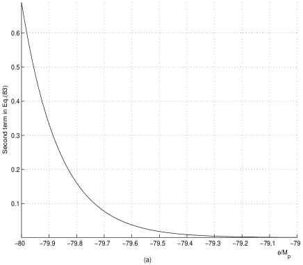
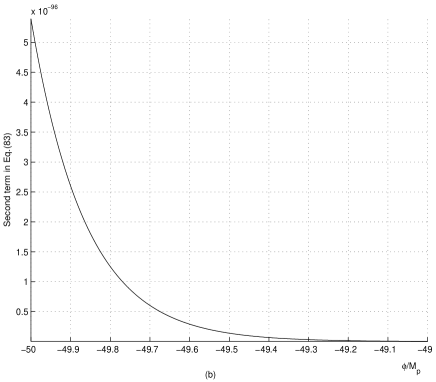
Figure 27: Behavior of the second term $I\equiv C_{2}Y_{\nu}\left(\beta e^{\alpha\varphi}\right)\cdot exp\left[-\left(\frac{3}{4\alpha^{2}}-\frac{\alpha}{2}\right)\varphi\right]$ in Eq.(90) is very singular: to provide the initial value of $I$ to be of the order of one as $\varphi_{in}=-80$ (Fig.(a)) we are forced to choose the value of the constant $C_{2}\sim 10^{-197}$. Then for example $I\sim 10^{-96}$ as $\varphi=-50$ (Fig.(b)).

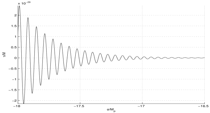
Figure 28: Here the analytic solution (91) has been used in order to zoom in on one of the five patterns of the phase trajectories shown in Figs.18a and 19. This graph illustrates a degree of damping of the Higgs field oscillations as $\varphi$ is close to -15 (i.e. near to the end of the interval where the solution (91) is applicable).

To compare this analytic solution with the results of the numeric solutions of subsection B we have used the same set of the values of the parameters (74) as in Sec.B. One can show that the graph of the first term proportional to $J_{\nu}\left(\beta e^{\alpha\varphi}\right)$ has the shape which for five sets of the initial conditions (75) results in the graphs which coincide with those in Fig.19. But the graph of the second term proportional to $Y_{\nu}\left(\beta e^{\alpha\varphi}\right)$ exhibits a very singular behavior, see Fig.27. Therefore when trying to satisfy the initial conditions with natural, i.e. non anomalously large values of $\tilde{\upsilon}(\varphi_{in})$ and $\left(d\tilde{\upsilon}/d\varphi\right)|_{\varphi=\varphi_{in}}$, we obtain that $C_{2}$ is very close to zero. Because of the extremely rapid decay of the second term, its contribution into the solution (90) quickly becomes negligible with growth of $\varphi$. Hence with very high accuracy one can proceed with the following analytic solution of Eq.(85):

$$\tilde{\upsilon}(\varphi)=C_{1}J_{\nu}\left(\beta e^{\alpha\varphi}\right)\cdot exp\left[-\left(\frac{3}{4\alpha^{2}}-\frac{\alpha}{2}\right)\varphi\right]$$ (91)

Choosing now the values of $C_{1}$ so that $\tilde{\upsilon}_{in}=\tilde{\upsilon}(\varphi_{in})$ equals to the initial values considered in the numerical solutions in Sec.VIIB, we obtain the same five graphs as in Figs.18a and 19 (but here only in the interval $\varphi\leq 15$). The curves $\tilde{\upsilon}(\varphi)$, which are the projections of the 4-dimensional phase trajectories on the $(\varphi,\tilde{\upsilon})$-plane, have the following characteristic features:

• From the beginning the solution $\tilde{\upsilon}(\phi)$ remains almost constant in a long enough $\phi$-interval, that corresponds to the GSB stage of the inflation The analytic solution (91) provides such a regime: the Bessel function of the first kind $J_{\nu}\left(\beta e^{\alpha\varphi}\right)$ starts from very small values and increases exponentially; it turns out that the decaying exponential factor in Eq.(91) compensates the growth of the Bessel function $J_{\nu}\left(\beta e^{\alpha\varphi}\right)$ with very high accuracy resulting in a very slow change of $\tilde{\upsilon}(\phi)$ during an initial long enough stage of the power law inflation (see Fig.18a). Note that in contrast to this the Bessel function of the second kind $J_{\nu}\left(\beta e^{\alpha\varphi}\right)$ decreases exponentially and therefore its product with the decaying exponential factor in Eq.(90) makes its relative contribution to the solution negligible very quickly.

• Analytic solutions $\tilde{\upsilon}(\phi)$ with different initial conditions fall to the same point $C$ of the line $\tilde{\upsilon}(\varphi)=0$, exactly as in the numerical solutions in Sec.VIIB, Figs.18a and 19. But now we have the mathematical explanation of this effect: the point $C$ is the first zero of the Bessel function. Since the choice of the initial value $\tilde{\upsilon}(\varphi_{in})$ determines only the appropriate value of the factor $C_{1}$ in Eq.(91), it becomes clear why independently of initial values $\tilde{\upsilon}(\varphi_{in})$ all the phase trajectories fall to the same point $C$.

• After the point $C$ (see Figs.18a, 19, 28) all the 4-dimensional phase trajectories approach the attractor $\left(\frac{d\varphi}{d\tau}=0,\,\tilde{\upsilon}=0,\,\frac{d\tilde{\upsilon}}{d\tau}=0\right)$ whose projection on the $(\varphi,\tilde{\upsilon})$-plane we observe in Figs.17a as the straight interval after the point $C(-32.8,0)$. As we see in Figs.19, 28, approaches to this attractor occur through the very strong damping of the oscillations of the Higgs field around its zero value. Note also that locations of all the zeros of the Bessel function $J_{\nu}\left(\beta e^{\alpha\varphi}\right)$ are determined only by the parameters of the model and are independent of the initial conditions.

After the point $(\varphi\approx-15,\tilde{\upsilon}=0)$, the presented analytic solution is not applicable since the inequality(79) does not hold for $\varphi>-15$ and therefore ignoring the back reaction of the Higgs field on the inflaton dynamics does not hold anymore.

The fall of all the phase trajectories (corresponding to different initial conditions) to the same point $C$ of the attractor $\tilde{\upsilon}=0$, along with the attractor behavior with respect to $\frac{d\varphi}{d\tau}=0$, has a decisive role in the observed effect: the magnitudes of $<\upsilon>^{2}$ and $\phi_{0}$ where $\upsilon$ and $\phi$ stop in the vacuum manifold (63) depend very weak of the initial conditions. In fact, if different phase trajectories would fall to different points of the attractor $\tilde{\upsilon}=0$ then the degree of damping of their oscillations right before they enter into the regime of the last phase transition (region $F$ in Fig.18a) could be generically very different. Those of them whose deviations from the attractor were not small would have the limiting point $(\phi_{0},<\upsilon>^{2})$ of the phase transition significantly different from others.

VII.4 Higgs-Inflaton Symbiosis: Comparison with Hybrid Inflation and Summary of the Main Features

The cosmological scenario studied in this section includes a number of dynamical effects demonstrating a strong enough tendency of the inflaton and Higgs fields to coexistence and interference. This is why we will refer to the appropriate phenomena as Higgs-Inflaton Symbiosis (HIS). The dynamics of the HIS model resembles the hybrid inflation modelLinde-hybrid but there are essential differences.

Hybrid inflation modelsLinde-hybrid contain more than one scalar fields one of which (the inflaton $\phi$) drives the early (long) stage of inflation and the dynamics of the other(s) determines the character of the final (very short) stage of inflation. One usually assumesLinde-hybrid that the extra scalar $\sigma$ is the Higgs field. Due to a direct inflaton-Higgs coupling the Higgs effective mass is $\phi$ dependent. During the early stage of inflation the Higgs effective mass square is positive and may be very large. This is the reason why the Higgs field is in the false vacuum $\sigma=0$ during the early stage of inflation. Afterwards, slow roll of the inflaton below a certain value causes the change of the sign of the Higgs effective mass square. In other words, the inflaton plays the role of a trigger which causes transition of the Higgs field into the true minimum of the scalar sector potential in the Higgs direction. This transition starts before the end of inflation because locations of the minima in the directions of the inflaton and the Higgs field do not coincide. The end of inflation and spontaneous breaking of the gauge symmetry appears to be intrinsically correlated: the last stages of inflation are supported not by the inflaton potential $V(\phi)$ but by the ”noninflationary” potential $V(\sigma)$. To provide a desirable scenario there is a need in strong enough restrictions on the parameters of the model. Note also that this type of models preserves the original feature of the standard approach to gauge symmetry breaking - the presence of a tachyonic mass term in the action.

Here we summarize the main features of the HIS model including a number of differences from hybrid inflation models.

• Incorporation of both the inflation and the gauge symmetry breaking is achieved without tachyonic mass terms in the original action (see Eqs.(9) and (56),(57)).

• The inflaton-Higgs coupling in Eq.(58) disappears in the inflationary epoch, i.e as the inflaton $\phi\ll-M_{p}$, see Eq.(59). Therefore the effective Higgs mass is constant during the inflation.

• The positivity of the effective mass square of the Higgs field in the inflationary epoch (see Eq.(59)) results directly from the positivity of the original mass square parameters $\mu_{1}^{2}$ and $\mu_{2}^{2}$ in the pre-potentials, Eqs.(56),(57).

• As a direct result of TMT, the effective scalar sector potential (58) has a structure which provides automatically a common location of the minima in the inflaton and the Higgs field directions. These minima form the line (63) in the plane $(\phi,\upsilon)$. Each point of this line describes a gauge symmetry broken state with zero vacuum energy density. Instead of resorting to tachyonic mass terms, these minima are achieved by assigning negative values to the constant parts $V_{1}^{(0)}$, $V_{2}^{(0)}$ of the pre-potentials, Eqs.(56),(57).

• Constancy of the effective Higgs mass during a significant part of the early stage of inflation allows for the Higgs field $\upsilon$ to remain practically equal to its initial value when the Hubble parameter is very large (GSB inflation).

• The fall of the Higgs field to the state $\upsilon=0$ (GSR inflation) occurs at a quite definite value of the e-folding before the end of inflation. This value of the e-folding is practically independent of the initial conditions.

• After falling to $\upsilon=0$ the Higgs field performs quickly damping oscillations around $\upsilon=0$.

• At the end of inflation (i.e. when $w=-1/3$) all the phase trajectories corresponding to different initial conditions appear to be very close to the attractor $\left(\frac{d\varphi}{d\tau}=0,\,\tilde{\upsilon}=0,\,\frac{d\tilde{\upsilon}}{d\tau}=0\right)$.

• The effective mass square of the Higgs field becomes negative after the end of inflation. Exponential form of the $\phi$ dependence in Eq.(58) makes this trigger effect very sharp. The demonstrated extreme closeness of all phase trajectories (corresponding to different initial conditions) to the attractor provides that the phase transition to the gauge symmetry broken phase occurs into a very short interval of the values of $<\upsilon>$ (and appropriate values of $\phi_{0}$) in the vacuum manifold(63).

• The remarkable structure of the scalar sector effective potential (58) (generated in the Einstein frame in our TMT model) automatically provides that the effective potential in the vacuum manifold (63) is equal to zero without fine tuning of the parameters of the action and the initial conditions.

• Note finally that in contrast with the hybrid inflation models where strong enough restrictions on the parameters are needed, in the HIS model qualitatively the same results are obtained in a very broad range of the parameters satisfying the conditions (57), (60).

VII.5 Particle Creation and Its Effects on Primordial Perturbations and
the Phase Transition: Qualitative Discussion

In the previous sections we did not touch quantum effects and their possible role in the studied processes. One of the most important quantum effects is the particle creation. Here we want to discuss on the qualitative level what kind of influence one can expect from the particle creation on the studied processes. In our qualitative discussion we have to take into account that in the HIS evolution there are two very different stages where oscillations of the Higgs field must cause matter creation.

(1) The first oscillatory stage consists of the transition from GSB to GSR inflation and the GSR inflation itself. A rapid transition of the Higgs field from a nonzero value to the $\upsilon=0$ phase has to be accompanied with particle creation. The subsequent coherent damping oscillations of the Higgs field around $\upsilon=0$, studied in detail in Secs.VIIB and VIIC must be responsible for creation of massless particles, like for example massless gauge bosons. This dissipative process results in an additional damping of the Higgs field oscillations. Hence the quantum effect of particle creation acts here as an additional factor which forces the phase trajectories corresponding to different initial conditions to achieve closer unification with the attractor $\left(\frac{d\varphi}{d\tau}=0,\,\tilde{\upsilon}=0,\,\frac{d\tilde{\upsilon}}{d\tau}=0\right)$. As a result of this the final values of $<\upsilon>$ and $\phi_{0}$ in the symmetry broken phase become more strongly independent of the initial conditions than in the pure classical model discussed in the preceding subsections.

One should note that with the chosen parameters, the reheating caused by the first stage of the particle creation can not play an essential role in the thermal history of the universe because it happens about 50 e-folding before the end of inflation. However possible effect of the appropriate thermal fluctuations on the primordial density perturbations perhaps deserves a special study.

(2) The second stage of the particle creation is realized after the end of inflation during the transition from $\tilde{\upsilon}=0$ phase to the gauge symmetry broken phase. Coherent oscillations of the Higgs field around the vacuum manifold discussed in detail in Sec. VIIB may serve as a very effective mechanism of the preheating, for example via gauge bosons creation. This effect has to be studied in detail, but it is beyond the goals of this paper. Nevertheless it is interesting to point out that the back reaction of the particle creation on the finish of the phase transition may be very important. Indeed, as we discussed in the preceding subsections, the characteristic feature of the final stage of the classical evolution of the Higgs-inflaton system is that the scalar sector energy density $\rho$ approaches zero. If there is no other matter, the friction $\sim\sqrt{\rho}$ caused by the cosmological expansion also approaches zero and therefore the finish of the classical evolution of the Higgs-inflaton system becomes problematic (see item 8 in Sec.VIIB). However, if one takes into account the quantum effects of matter creation due to the Higgs field oscillations around the vacuum manifold, this immediately produces additional friction in the Higgs field equation non related to the cosmological expansion. Besides, the presence of massive gauge bosons, photons and fermions in addition to the scalar sector (the energy density of the latter is very close to zero) means that the universe has entered into a radiation/matter dominated era. Therefore the friction caused by the cosmological expansion (both in the inflaton and in the Higgs field equations) is now $\sim\sqrt{\rho_{tot}}$ where $\rho_{tot}$ includes also the radiation/matter energy density. Due to these two back reaction effects the Higgs and inflaton fields must quickly dissipate their kinetic energy and the evolution of the Higgs-inflaton system has to finish in a certain point of the vacuum manifold which is practically independent of the initial conditions.

One should finally point out that in this paper we have restricted ourselves only with a homogeneous distribution of the initial values of the Higgs field. However the discussed practical independence of $<\upsilon>$ of the initial conditions in the framework of the homogeneous problem may serve as an indication that in a more realistic case of inhomogeneous distribution of the initial values of the Higgs field, its value in the final gauge symmetry broken phase will be practically the same everywhere in our universe.

VIII Discussion and Conclusion

VIII.1 Differences of TMT from the standard field theory in curved space-time

The main idea of TMT is that the general form of the action $\int L\sqrt{-g}d^{4}x$ is not enough in order to account for some of the fundamental problems of particle physics and cosmology. The key difference of TMT from the standard field theory in curved space-time consists in the hypothesisGK1 -GK3 that in addition to the term in the action with the volume element $\sqrt{-g}d^{4}x$ there should be one more term where the volume element is metric independent but rather it is determined either by four (in the 4-dimensional space-time) scalar fields $\varphi_{a}$ or by a three index potential $A_{\alpha\beta\gamma}$, see Eqs.(1)-(3). We would like to emphasize that including in the action of TMT the coupling of the Lagrangian density $L_{1}$ with the measure $\Phi$, we modify in general both the gravitational and matter sectors as compared with the standard field theory in curved space-time. Besides we made two more assumptions: the measure fields ($\varphi_{a}$ or $A_{\alpha\beta\gamma}$) appear only in the volume element; one should proceed in the first order formalism. These assumptions constitute all the modifications of the general structure of the theory we have made as compared with the standard field theory in curved space-time. In fact, the Lagrangian densities $L_{1}$ and $L_{2}$ in the models we have studied in the present paper, contain all types of terms which should be present if the standard model would be formulated in curved space-time. However we do not consider any exotic terms and it turns out that there is no need for any exotic term in order to achieve desirable results. In particular there is no need for the phantom type terms in $L_{1}$ and $L_{2}$ in order to obtain super-acceleration at the late time universe; there is no need for tachyonic mass terms in the Higgs pre-potentials $V_{1}$ and $V_{2}$ in order to obtain spontaneous breakdown of gauge symmetry.

After making use of the variational principle and formulating the resulting equations in the Einstein frame, we have seen that in the absence of fermions, the dynamics of the scalar sector is described by the effective action (44) which is a concrete realization of the $k$-essencek-essence obtained from first principles.

VIII.2 Short summary of results

VIII.2.1 The early universe inflation

For pedagogical reasons in Secs.IV-VI we have studied first models without Higgs field. As $\delta=0$, the dynamics of $\phi$ can be analyzed by means of its effective potential (48). As $\phi\ll-M_{p}$ the effective $\phi$ potential has the exponential form. We have seen that independently of the values of the parameters $V_{1}$, $V_{2}$ and under very general initial conditions, solutions rapidly approach a regime characterized by a power law inflation. If $\delta\neq 0$, we deal with the intrinsically $k$-essence dynamics. The numerical solutions in this case have showed that there is no qualitative difference of the power law inflation from the case with $\delta=0$.

For the model with the Higgs field and $\delta=0$, we have seen that with the choice of positive mass squared parameters $\mu_{1}^{2}$ and $\mu_{2}^{2}$, the effective potential of the scalar sector in the very early universe, Eq.(59), describes the Higgs field with positive mass square, i.e. the minimization of the effective potential (59) in the Higgs direction in the inflationary epoch is achieved if the Higgs field is in the unbroken symmetry phase $\upsilon=0$. The inflationary epoch with $\upsilon=0$ we called the GSR inflation. However in contrast with the hybrid inflationLinde-hybrid , before the GSR inflation the universe suffers a long lasting GSB inflation, where the Higgs field is in a broken gauge symmetry phase with slow varying $\upsilon\neq 0$. With our choice of the parameters, the transition from the GSB inflation to the GSR inflation occurs about 60 e-folding before the end of inflation, see Fig.22.

VIII.2.2 End of inflation in models without the Higgs field

In these toy models there are three regions of the parameters $V_{1}$ and $V_{2}$ and appropriate three shapes of the effective potentials, Fig.1. Therefore three different types of scenarios for exit from inflation can be realized:

a) $V_{1}>0$ and $b_{g}V_{1}>2V_{2}$,   Sec.IV. In this case the power law inflation monotonically transforms to the late time inflation asymptotically governed by the cosmological constant $\Lambda_{1}$.

b) $V_{2}<b_{g}V_{1}<2V_{2}$,   Sec.V. In this case the power law inflation is ended without oscillations at the final value $\phi_{min}$, corresponding to the (non zero) minimum of the effective potential,.

c) $V_{1}<0$ and $V_{2}<0$,   Sec.VI. In this case the power law inflation is ended with damped oscillations of $\phi$ approaching the point of the phase plane ($\phi=\phi_{0},\dot{\phi}=0$) where the vacuum energy $V_{eff}^{(0)}(\phi_{0})=0$. This occurs without fine tuning of the parameters $V_{1}$, $V_{2}$, $\delta$ and the initial conditions.

VIII.2.3 New cosmological mechanism for gauge symmetry breaking
and reheating

.

From the summary of the main features of the HIS (see Sec. VIID) one can conclude that our TMT model implies a new cosmological mechanism for a transition to a gauge symmetry broken phase soon after the end of inflation. From the field theory point of view, one of the advantages of the model is that the gauge symmetry breaking is obtained without tachyonic mass terms in the original action. Another important advantage of the model is that the inflaton driven transition to the the gauge symmetry broken phase is automatically (i.e. without tuning) accompanied with approaching zero of the scalar sector energy density. From the point of view of the realistic cosmology, the scenario based on the HIS model exhibits a new mechanism of reheating which most likely may be very effective: coherent oscillations of the Higgs field must result in intensive creation of the gauge bosons. Besides, transition to the gauge symmetry broken phase starts soon after the end of the GSR inflation where $\upsilon=0$ and therefore masses of quantum of all the gauge fields are very close to zero at the beginning of the reheating.

VIII.2.4 Cosmological constant problems

The old cosmological constant problem. In Secs.VI and VII, we have seen in details that if $V_{1}<0$ then, for a broad range of other parameters, the vacuum energy turns out to be zero without fine tuning; this is possible both in the model with $\phi$ as the scalar sector and in the model with $\phi$ and $\upsilon$. This effect is a direct consequence of the result of the TMT: the effective scalar sector potential generated in the Einstein frame is proportional to a perfect square. If such type of the structure for the scalar field potential in a usual (non TMT) model would be chosen ”by hand” it would be a sort of fine tuning.

There is a need to explain how this result avoids the well known no-go theorem by WeinbergWeinberg1 stating that generically in field theory one cannot have zero value of the potential in the minimum without fine tuning. The reason why this theorem is not applicable here is that one of the basic assumptions of the theorem does not hold. Indeed in the mentioned theorem, it is assumed that all fields in the vacuum are constants. In our case, the basic assumption that the measure of integration in the action $\Phi\neq 0$ implies that all the measure fields ($\varphi_{a}$ ($a=1,2,3,4$) in the definition (2) or $A_{\alpha\beta\gamma}$ in the definition (3)) have non vanishing space-time gradients.

In this paper we have restricted ourselves with the simplest form (56) of the Higgs field dependence of the pre-potentials $V_{1}$ and $V_{2}$. If however we had studied models with more complicated Higgs field dependence in $V_{1}$ and $V_{2}$, including for example the quartic Higgs self-interactions, then there could be vacua with zero cosmological constant disconnected from each other (again without fine tuning). This is an explicit realization of the ”Multiple Point Principle” proposalNielsen which is based on the idea that if there is a mechanism that sets a certain state to have a zero cosmological constant then the same mechanism may act also in other field configurations with the same result.

The new cosmological constant problem.

Interesting result following from the general structure of the scale invariant TMT model with $V_{1}>0$ is that the cosmological constant $\Lambda_{1}$, Eq.(52), is a ratio of quantities constructed from pre-potentials $V_{1}$, $V_{2}$ and the dimensionless parameter $b_{g}$. Such structure of $\Lambda_{1}$ allows to propose at least two independent ways (see Sec.IV) for resolution of the problem of the smallness of $\Lambda_{1}$ that should be $\Lambda_{1}\sim(10^{-3}eV)^{4}$.

The first way is a kind of a seesaw mechanismseesaw . For instance, if $V_{1}\sim(10^{3}GeV)^{4}$ and $V_{2}\sim(10^{18}GeV)^{4}$ then $\Lambda_{1}\sim(10^{-3}eV)^{4}$.

The second way is realized if the dimensionless parameters $b_{g}$, $b_{\phi}$, etc. of the action (9) are huge numbers. For example, if $V_{1}\sim(10^{3}GeV)^{4}$ then for getting $\Lambda_{1}\sim(10^{-3}eV)^{4}$ one should assume that $b_{g}\sim 10^{60}$. It is interesting that this idea may be treated as an indication that there is a connection between the resolution of the new cosmological constant problem and a new type of the correspondence principle in the action, see details in item (b) of Sec.IV.

VIII.2.5 Possibility of the late time super-acceleration. Speculations about realistic cosmological scenario.

We have seen in this paper that even restricting ourselves with only the scalar sector we discover a number of interesting effects which may be useful in the construction of a realistic scenario of the evolution of the universe. Studying these effects makes it difficult in the same paper to address also questions like particle creation, perturbations, etc.. For this reason we cannot yet present a more complete cosmological scenario. In particular, we have seen in Sec.V that there is a region of the parameters where the late time universe can evolve with equation-of-state $w<-1$ without introducing explicit phantom terms in the action. This occurs due to the very interesting effect of the classical field dynamics described in Sec.V in detail. However it is impossible to obtain a pure classical solution which connects the early universe inflation with the late time super-acceleration. This problem may be related with the toy character of the scenario where the role of the matter has been ignored.

In TMT, the effects related to particle creation can change the dynamics of the scalar sector. In fact, if the particle creation results in the matter domination epoch, then in the presence of fermions, the constraint (29) differs from the constraint in the absence of fermions, Eq.(33). Therefore in the stage of a transition from the scalar sector (dark energy) domination epoch to the matter domination epoch, $\zeta$ must significantly vary that will lead to a change in the dynamics of the scalar sector due to the $\zeta$-dependence of the scalar sector potential (20). Similar conclusion is true also for the dynamics of the scalar sector in the matter domination epoch itself. In such a case the matter creation and subsequent matter domination epoch might be ”bridges” connecting the early inflation with the possible late time super-acceleration. This should include also a so far unclear mechanism responsible for the freezing of the Higgs vacuum expectation value $<\upsilon>$ to survive till the late time universe. This kind of questions we are going to study in the near future.

VIII.3 What can we expect from quantization

In this paper we have studied only classical two measures field theory and its effects in the context of cosmology. However quantization of TMT as well as influence of quantum effects on the processes explored in this paper may have a crucial role. We summarize here some ideas and speculations which gives us a hope that quantum effects can keep and even strengthen the main results of this paper.

1) Recall first two fundamental facts of TMT as a classical field theory: (a) The measure degrees of freedom appear in the equations of motion only via the scalar $\zeta$, Eq.(7); (b) The scalar $\zeta$ is determined by the constraint which is nothing but a consistency condition of the equations of motion (see Eqs.(92), (95) and (96) in Appendix B). Therefore the constraint plays a key role in TMT. Note however that if we were ignore the gravity from the very beginning in the action (9) then instead of the constraint (96) we would obtain Eq.(92) (where one has to put zero the scalar curvature). In such a case we would deal with a different theory. This notion shows that the gravity and matter intertwined in TMT in a much more complicated manner than in GR. Hence introducing the new measure of integration $\Phi$ we have to expect that the quantization of TMT may be a complicated enough problem. Nevertheless we would like here to point out that in the light of the recently proposed idea of Ref.Giddings , the incorporation of four scalar fields $\varphi_{a}$ together with the scalar density $\Phi$, Eq.(2), (which in our case are the measure fields and the new measure of integration respectively), is a possible way to define local observables in the local quantum field theory approach to quantum gravity. We regard this result as an indication that the effective gravity $+$ matter field theory has to contain the new measure of integration $\Phi$ as it is in TMT.

2) The assumption formulated in item 2 in Sec.IIA, that the measure fields $\varphi_{a}$ (or $A_{\alpha\beta\gamma}$) appear in the action (1) only via the measure of integration $\Phi$, has a key role in the TMT results and in particular for the resolution of the old cosmological constant problem, see Sec.VI. In principle one can think of breakdown of such a structure by quantum corrections. However, fortunately there exists an infinite dimensional symmetry mentioned in item 2 of Sec.IIA which, as we hope, is able to protect the postulated structure of the action from a deformation caused by quantum corrections or at least to suppress such a quantum anomaly in significant degree. Therefore one can hope that the proposed resolution of the old cosmological constant problem holds in the quantized TMT as well.

3) As we have noticed in Sec.VIIA, the vacuum manifold (63) of the HIS is degenerate: the effective potential of the scalar sector remains equal to zero when shifting along this line in the $(\phi,\upsilon)$ plane. However this degeneracy has no relation to any symmetry of the action, and in particular the kinetic energy of the scalar sector does not respect this shift as a symmetry. Therefore there are no reasons for quantum corrections not to break this shift symmetry of the vacuum manifold. Disappearance of the degeneracy of the vacuum manifold provides us with two important conclusions: a) our model is out of danger to run against the problem of the appearance of a pseudo-Goldstone boson; b) transition to the gauge symmetry broken phase will end in a certain point $(\phi_{0},<\upsilon>^{2})$ instead of a short interval of the line (63) as it was in the pure classical problem studied in Sec.VII.

4) Recall finally that such quantum effects as the first and the second stages of particle creation discussed in details in Sec.VIIE, supplement and strengthen the obtained classical results: the first stage of particle creation allows to hope that VEV of the Higgs field is independent of the initial conditions; the second stage of particle creation should work as a mechanism of dissipation responsible for realization of the final state of the HIS in the gauge symmetry broken phase.

Exploration of the quantization problems of TMT will be the subject of forthcoming research.

IX Acknowledgements

We thank L. Amendola, S. Ansoldi, R. Barbieri, J. Bekenstein, A. Buchel, A. Dolgov, S.B. Giddings, P. Gondolo, J.B. Hartle, B-L. Hu, P.Q. Hung, D. Kazanas, D. Marolf, D.G. McKeon, J. Morris, V. Miransky, H. Nielsen, Y.Jack Ng, H. Nishino, E. Nissimov, S. Pacheva, L. Parker, R. Peccei, M. Pietroni, S. Rajpoot, R. Rosenfeld, V. Rubakov, E. Spallucci, A. Vilenkin, S. Wetterich and A. Zee for helpful conversations on different stages of this research. Our special gratitude to M. Gedalin for his advice concerning some questions of dynamical systems and to L. Prigozhin for great help in implementation of numerical solutions.

Appendix A Equations of motion in the original frame

Variation of the measure fields $\varphi_{a}$ with the condition $\Phi\neq 0$ leads, as we have already seen in Sec.II, to the equation $L_{1}=sM^{4}$ where $L_{1}$ is now defined, according to Eq. (1), as the part of the integrand of the action (9) coupled to the measure $\Phi$. Equation (5) in the context of the model (9) reads (with the choice $s=1$):

$$\left[-\frac{1}{\kappa}R(\omega,e)+\frac{1}{2}g^{\mu\nu}\phi_{,\mu}\phi_{,\nu}+\frac{1}{2}g^{\mu\nu}(D_{\mu}H)^{{\dagger}}D_{\nu}H\right]e^{\alpha\phi/M_{p}}-V_{1}e^{2\alpha\phi/M_{p}}+L_{fk}e^{\alpha\phi/M_{p}}$$

$$-\frac{\upsilon}{\sqrt{2}}\left[f_{N}\overline{N}N+f_{E}\overline{E}E\right]=M^{4},$$ (92)

where the representation of the Higgs field $H$ in the unitary gauge

$$H=\begin{pmatrix}0\\ 2^{-1/2}\upsilon(x)\end{pmatrix}$$ (93)

has been used in the last term of the l.h.s. of Eq.(92); to simplify the coming calculations it is convenient in the meanwhile not to do this explicitly with $D_{\mu}H$ which includes interactions to gauge fields.

It can be noticed that the appearance of a nonzero integration constant $M^{4}$ spontaneously breaks the scale invariance (8).

Variation of the action (9) with respect to $e^{a\mu}$ yields

$$(\zeta+b_{g})\left[-\frac{2}{\kappa}R_{a,\mu}(\omega,e)+e^{\beta}_{a}(D_{\mu}H)^{{\dagger}}D_{\beta}H\right]+(\zeta+b_{\phi})e^{\beta}_{a}\phi_{,\mu}\phi_{,\beta}+\frac{1}{\sqrt{-g}}\frac{\partial(\sqrt{-g}L_{gauge})}{\partial e^{a,\mu}}e^{-\alpha\phi/M_{p}}$$ (94)

$$+ g_{\mu\beta}e^{\beta}_{a}\left[\frac{b_{g}}{\kappa}R(\omega,e)-\frac{b_{\phi}}{2}g^{\mu\nu}\phi_{,\mu}\phi_{,\nu}-\frac{b_{g}}{2}g^{\mu\nu}(D_{\mu}H)^{{\dagger}}D_{\nu}H+V_{2}e^{\alpha\phi/M_{p}}\right]$$

$$+ g_{\mu\beta}e^{\beta}_{a}\left[-kL_{fk}+\frac{\upsilon}{\sqrt{2}}\left(h_{N}f_{N}\overline{N}N+h_{E}f_{E}\overline{E}E\right)e^{\frac{1}{2}\alpha\phi/M_{p}}\right]$$

$$+ (\zeta+b)\frac{i}{2}\left[\overline{L}_{L}\left(\gamma^{a}\overrightarrow{D}_{\mu}-\overleftarrow{D}_{\mu}\gamma^{a}\right)L_{L}+\overline{E}_{R}\left(\gamma^{a}\overrightarrow{D}_{\mu}-\overleftarrow{D}_{\mu}\gamma^{a}\right)E_{R}+\overline{N}_{R}\left(\gamma^{a}\overrightarrow{D}_{\mu}-\overleftarrow{D}_{\mu}\gamma^{a}\right)N_{R}\right]=0.$$

Contraction of Eq.(94) with $e^{a,\mu}$ gives

$$(\zeta-b_{g})\left[-\frac{1}{\kappa}R(\omega,e)++\frac{1}{2}g^{\mu\nu}(D_{\mu}H)^{{\dagger}}D_{\nu}H\right]+(\zeta-b_{\phi})\frac{1}{2}g^{\mu\nu}\phi_{,\mu}\phi_{,\nu}+2V_{2}e^{\alpha\phi/M_{p}}+\frac{1}{2}(\zeta-3k)L_{fk}$$ (95)

$$+ \frac{2\upsilon}{\sqrt{2}}\left(h_{N}f_{N}\overline{N}N+h_{E}f_{E}\overline{E}E\right)e^{\frac{1}{2}\alpha\phi/M_{p}}=0,$$

where the identity $e^{a\mu}\left(\partial\sqrt{-g}L_{gauge}/\partial e^{a\mu}\right)\equiv 0$ has been used.

Excluding $R(\omega,e)$ from Eqs.(92) and (95) we obtain the consistency condition of these two equations:

$$(\zeta-b_{g})\left(M^{4}e^{-\alpha\phi/M_{p}}+V_{1}e^{\alpha\phi/M_{p}}\right)+2V_{2}e^{\alpha\phi/M_{p}}+(b_{g}-b_{\phi})\frac{1}{2}g^{\mu\nu}\phi_{,\mu}\phi_{,\nu}-\frac{1}{2}(\zeta-2b_{g}+3k)L_{fk}$$ (96)

$$+ \frac{\upsilon}{\sqrt{2}}\left[(\zeta-b_{g}+2h_{N})f_{N}\overline{N}N+(\zeta-b_{g}+2h_{E})f_{E}\overline{E}E)\right]e^{\frac{1}{2}\alpha\phi/M_{p}}=0,$$

It is well known that the Lagrangian for a single fermion field $\Psi$ equals zero on the mass-shell. This results from the linearity of the Lagrangian both in $\Psi$ and in $\overline{\Psi}$. The same is true for a system of fermion fields in our case because in spite of the presence of interactions, the fermion sector in (9) is linear in all fermion degrees of freedom. Therefore we have

$$(\zeta+k)L_{fk}=\frac{\upsilon}{\sqrt{2}}\left[(\zeta+h_{N})f_{N}\overline{N}N+(\zeta+h_{E})f_{E}\overline{E}E\right]e^{\frac{1}{2}\alpha\phi/M_{p}}$$ (97)

Inserting $L_{fk}$ into the consistency condition, Eq.(96), we get the constraint (in the original frame)

$$(\zeta-b_{g})\left(M^{4}e^{-2\alpha\phi/M_{p}}+V_{1}\right)+2V_{2}+(b_{g}-b_{\phi})e^{-\alpha\phi/M_{p}}\frac{1}{2}g^{\mu\nu}\phi_{,\mu}\phi_{,\nu}$$ (98)

$$+ \frac{\upsilon}{2\sqrt{2}(\zeta+k)}e^{-\frac{1}{2}\alpha\phi/M_{p}}\sum_{i=N,E}(\zeta-\zeta_{1}^{(i)})(\zeta-\zeta_{1}^{(2)})\overline{\Psi}_{i}\Psi_{i}=0.$$

where $\Psi_{i}$ ($i=N,E$) is the general notation for the primordial fermion fields $N$ and $E$ and

$$\zeta_{1,2}^{(i)}=\frac{1}{2}\left[k-3h_{i}\pm\sqrt{(k-3h_{i})^{2}+8b_{g}(k-h_{i})-4kh_{i}}\,\right],\qquad i=N,E.$$ (99)

Contracting Eq.(94) with factor $e^{a}_{\nu}$ and using Eqs.(95), (97) we get

$$\frac{2}{\kappa}R_{\mu\nu}(\omega,e) = \frac{\zeta+b_{\phi}}{\zeta+b_{g}}\phi_{,\mu}\phi_{,\nu}+(D_{\mu}H)^{{\dagger}}D_{\nu}H+\frac{2}{\sqrt{-g}}\frac{\partial\sqrt{-g}L_{gauge}}{\partial g_{\mu\nu}}e^{-\alpha\phi/M_{p}}$$ (100)

$$- g_{\mu\nu}\frac{1}{\zeta+b_{g}}\left[b_{g}M^{4}e^{-\alpha\phi/M_{p}}+(b_{g}V_{1}-V_{2})e^{\alpha\phi/M_{p}}-(b_{g}-b_{\phi})\frac{1}{2}g^{\alpha\beta}\phi_{,\alpha}\phi_{,\beta}\right]$$

$$+ \frac{\zeta+k}{\zeta+b_{g}}\frac{i}{2}e_{a\nu}\left[\overline{L}_{L}\left(\gamma^{a}\overrightarrow{D}_{\mu}-\overleftarrow{D}_{\mu}\gamma^{a}\right)L_{L}+\overline{E}_{R}\left(\gamma^{a}\overrightarrow{D}_{\mu}-\overleftarrow{D}_{\mu}\gamma^{a}\right)E_{R}+\overline{N}_{R}\left(\gamma^{a}\overrightarrow{D}_{\mu}-\overleftarrow{D}_{\mu}\gamma^{a}\right)N_{R}\right]$$

$$+ g_{\mu\nu}\frac{\upsilon}{\sqrt{2}(\zeta+k)}e^{\frac{1}{2}\alpha\phi/M_{p}}\left[(h_{N}-k)f_{N}\overline{N}N+(h_{E}-k)f_{E}\overline{E}E\right].$$

The scalar field $\phi$ equation of motion in the original frame can be written in the form

$$\frac{1}{\sqrt{-g}}\partial_{\mu}\left[e^{\alpha\phi/M_{p}}(\zeta+b_{\phi})\sqrt{-g}g^{\mu\nu}\partial_{\nu}\phi\right]$$ (101)

$$- \frac{\alpha}{M_{p}}e^{\alpha\phi/M_{p}}\left[(\zeta+b_{g})M^{4}e^{-\alpha\phi/M_{p}}+[(b_{g}-\zeta)V_{1}-2V_{2}]e^{\alpha\phi/M_{p}}+(b_{g}-b_{\phi})\frac{1}{2}g^{\alpha\beta}\phi_{,\alpha}\phi_{,\beta}\right]$$

$$= -\frac{\alpha}{M_{p}}e^{\frac{3}{2}\alpha\phi/M_{p}}\frac{\upsilon}{2\sqrt{2}(\zeta+k)}\sum_{i=N,E}(\zeta-\zeta_{1}^{(i)})(\zeta-\zeta_{1}^{(2)})\overline{\Psi}_{i}\Psi_{i},$$

where Eqs.(92) and (97) have been used.

In the vacuum of the gauge fields, the Higgs field equation in the unitary gauge reads

$$\frac{1}{\sqrt{-g}}\partial_{\mu}\left[e^{\alpha\phi/M_{p}}(\zeta+b_{g})\sqrt{-g}g^{\mu\nu}\partial_{\nu}\upsilon\right]+e^{2\alpha\phi/M_{p}}[\zeta V^{\prime}_{1}+V^{\prime}_{2}]=-\frac{\upsilon}{\sqrt{2}}\,e^{\frac{3}{2}\alpha\phi/M_{p}}\sum_{i=N,E}f_{i}(\zeta+h_{i})\overline{\Psi}_{i}\Psi_{i},$$ (102)

where $V_{i}^{\prime}\equiv dV_{i}/d\upsilon$, $(i=1,2)$.

The gauge field $B_{\mu}$ equation in the unitary gauge and in the fermion vacuum reads

$$\partial_{\nu}\left[\sqrt{-g}g^{\alpha\mu}g^{\beta\nu}B_{\alpha\beta}\right]+e^{\alpha\phi/M_{p}}(\zeta+b_{g})\sqrt{-g}g^{\mu\nu}\frac{1}{8}g^{\prime 2}\upsilon^{2}B_{\nu}=0$$ (103)

and similar for $\vec{W}_{\mu}$.

The fermion $\Psi_{i}$ equation in the unitary gauge and for simplicity, in the gauge fields vacuum has the following form

$$ie_{a}^{\mu}\left[\gamma^{a}\vec{\partial}_{\mu}+\frac{1}{4}\omega_{\mu}^{cd}\left(\gamma^{a}\sigma_{cd}+\sigma_{cd}\gamma^{a}\right)\right]\Psi_{i}+\frac{ie^{-\alpha\phi/M_{p}}}{2(\zeta+k)\sqrt{-g}}\left[\partial_{\mu}\left((\zeta+k)\sqrt{-g}e^{\alpha\phi/M_{p}}e_{a}^{\mu}\right)\right]\gamma^{a}\Psi_{i}$$ (104)

$$- \frac{\zeta+h_{i}}{\zeta+k}e^{\frac{1}{2}\alpha\phi/M_{p}}\frac{f_{i}\upsilon}{\sqrt{2}}\Psi_{i}=0.$$

Appendix B Connection in the original and Einstein frames

We present here what is the dependence of the spin connection $\omega_{\mu}^{ab}$ on $e^{a}_{\mu}$, $\zeta$, $\Psi$ and $\overline{\Psi}$. Varying the action (9) with respect to $\omega_{\mu}^{ab}$ and making use that

$$R(V,\omega)\equiv-\frac{1}{4\sqrt{-g}}\varepsilon^{\mu\nu\alpha\beta}\varepsilon_{abcd}e^{c}_{\alpha}e^{d}_{\beta}R_{\mu\nu}^{ab}(\omega)$$ (105)

we obtain

$$\varepsilon^{\mu\nu\alpha\beta}\varepsilon_{abcd}\left[(\zeta+b_{g})e^{c}_{\alpha}D_{\nu}e^{d}_{\beta}+\frac{1}{2}e^{c}_{\alpha}e^{d}_{\beta}\left(\zeta_{,\nu}+\frac{\alpha}{M_{p}}\phi_{,\nu}\right)\right]+\frac{\kappa}{4}\sqrt{-g}(\zeta+k)e^{c\mu}\varepsilon_{abcd}\overline{\Psi}\gamma^{5}\gamma^{d}\Psi=0,$$ (106)

where

$$D_{\nu}e_{a\beta}\equiv\partial_{\nu}e_{a\beta}+\omega_{\nu a}^{d}e_{d\beta}$$ (107)

The solution of Eq. (106) is represented in the form

$$\omega_{\mu}^{ab}=\omega_{\mu}^{ab}(e)+K_{\mu}^{ab}(e,\overline{\Psi},\Psi)+K_{\mu}^{ab}(\zeta,\phi)$$ (108)

where

$$\omega_{\mu}^{ab}(e)=e_{\alpha}^{a}e^{b\nu}\{^{\alpha}_{\mu\nu}\}-e^{b\nu}\partial_{\mu}e_{\nu}^{a}$$ (109)

is the Riemannian part of the spin-connection,

$$K_{\mu}^{ab}(e,\overline{\Psi},\Psi)=\frac{\kappa}{8}\frac{\zeta+k}{\zeta+b_{g}}\eta_{cn}e_{d\mu}\varepsilon^{abcd}\overline{\Psi}\gamma^{5}\gamma^{n}\Psi$$ (110)

is the fermionic contribution that differs from the familiar one ..,Gasperini by the factor $\frac{\zeta+k}{\zeta+b_{g}}$ and

$$K_{\mu}^{ab}(\zeta,\phi)=\frac{1}{2(\zeta+b_{g})}\left(\zeta_{,\alpha}+\frac{\alpha}{M_{p}}\phi_{,\alpha}\right)(e_{\mu}^{a}e^{b\alpha}-e_{\mu}^{b}e^{a\alpha})$$ (111)

is the non-Riemannian part of the spin-connection originated by specific features of TMT.

In the Einstein frame, i.e. in terms of variables defined by Eq.(16), the spin-connection read

$$\omega^{\prime ab}_{\mu}=\omega^{ab}_{\mu}(\tilde{e})+\frac{\kappa}{8}\eta_{cn}\tilde{e}_{d\mu}\varepsilon^{abcd}\overline{\Psi}^{\prime}\gamma^{5}\gamma^{n}\Psi^{\prime}$$ (112)

which is exactly the spin-connection of the Einstein-Cartan space-timeGasperini with the vierbein $\tilde{e}^{a}_{\mu}$.

Appendix C General Relativity and Regular Fermions

C.1 Reproducing Einstein Equations and Regular Fermions

In Sec.III we have seen that in the absence of fermions case (and if $\delta=0$) the gravitational equations (18) coincide with the Einstein equations. Analyzing Eqs.(18)-(23) in more general cases it is easy to see that Eqs.(18) and (19) are reduced to the Einstein equations in the appropriate field theory model (i.e. when the scalar field, electromagnetic field and massive fermions are sources of gravity) if $\zeta$ is constant and

$$\Lambda_{dyn}^{ferm}=0\qquad\text{or at least}\qquad|T_{\mu\nu}^{(ferm,noncan)}|\ll|T_{\mu\nu}^{(ferm,can)}|.$$ (113)

According to Eqs.(21)-(23), in the case when a single massive fermion is a source of gravity, the condition (113) is realized if

$$Z_{i}(\zeta)\approx 0\quad\Longrightarrow\quad\zeta=\zeta_{1}^{i}\quad or\quad\zeta=\zeta_{2}^{i},\quad i=N^{\prime},E^{\prime},$$ (114)

where $\zeta_{1,2}^{i}$ are defined in Eqs.(22).

Recall that existence of a noncanonical contribution to the energy-momentum tensor (21), along with the $\zeta$ dependence of the fermion mass (23) discovered in Sec.IIC, displays the fact that generically primordial fermion is very much different from the regular one (see definitions in item (ii) of the Introduction section). To answer the question what are the characteristic features of the regular massive fermion we have to take into account the undisputed fact that the classical tests of GR deal only with regular fermionic matter. Hence we should identify the regular fermions with states of the primordial fermions satisfying the condition (114).

C.2 Meaning of the Constraint and Regular Fermions

We are going now to understand the meaning of the constraint (29). We start from the detailed analysis of two limiting cases: (a) in space-time regions without fermions;   (b) in space-time regions occupied by regular fermions;   and afterwards we will be able to formulate the meaning of the constraint in general case.

We will proceed choosing the parameters $V_{1}$, $V_{2}$ and/or $b_{g}$ as in Sec.IV. It is convenient to divide the analysis into a few steps:

(1) It follows from the condition $b_{g}V_{1}>2V_{2}$ that $\zeta_{0}(\phi)$ determined by the constraint in the absence of fermions case, Eq.(46), has the same order of magnitude as the parameter $b_{g}$.

(2) Recall that $V_{eff}^{(0)}(\phi)$, Eq.(48), having the order of magnitude typical for the dark energy density (in the absence of fermions case) is obtained from $V_{eff}(\phi;\zeta)$, Eq.(20), as $\zeta=\zeta_{0}(\phi)$. Therefore with the help of the item (1) we conclude that each time when $\zeta$ has the order of magnitude close to that of the parameter $b_{g}$ (and if no special tuning is assumed) $V_{eff}(\phi;\zeta)$, Eq.(20), has the order of magnitude close to that of the dark energy density (in the absence of fermions case).

(3) It is easy to see that each time when $\zeta$ has the order of magnitude close to that of the parameter $b_{g}$ (if no special tuning is assumed and in particular $\zeta\neq\zeta_{0}(\phi)$), the left hand side (l.h.s.) of the constraint (29) has the order of magnitude close to that of $V_{eff}(\phi;\zeta)$, Eq.(20), i.e. the l.h.s. of the constraint has the order of magnitude close to that of the dark energy density in the absence of fermions case.

(4) Let us now turn to the right hand side (r.h.s.) of the constraint (29) in the presence of a single massive primordial fermion. It contains factor $m_{i}(\zeta)\overline{\Psi}^{\prime}_{i}\Psi^{\prime}_{i}$,   ($i=N^{\prime},E^{\prime}$) which have typical order of magnitude of the fermion canonical energy density $T_{00}^{(ferm,can)}$. If the primordial fermion is in a state of a regular fermion then according to the conclusion made at the end of the previous subsection, in the space-time region where the fermion is localized, the scalar $\zeta$ must be $\zeta=\zeta_{1}^{i}$ (or $\zeta=\zeta_{2}^{i}$). Therefore in the space-time region occupied by a single regular fermion, the r.h.s. of (29) is

$$\Lambda_{dyn}^{(ferm)}|_{regular}\equiv Z_{i}(\zeta_{1,2}^{i})m_{i}(\zeta_{1,2}^{i})\left(\overline{\Psi^{\prime}_{i}}\Psi^{\prime}_{i}\right)_{regular}$$ (115)

Due to our assumption that the dimensionless parameters $b_{g}$, $b_{\phi}$, $k$, $h_{N}$ and $h_{E}$ have close orders of magnitude (see paragraph after Eq.(15)), it follows from the definitions (22) that both $\zeta_{1}^{i}$ and $\zeta_{2}^{i}$ have the order of magnitude close to that of $b_{g}$. Hence in the space-time region occupied by a single regular fermion, the l.h.s. of (29) has the order of magnitude close to that of the dark energy density in the fermion vacuum. It is evident that in normal particle physics conditions (see the last paragraph of Sec.II), that is when the energy density of a single fermion $\sim m_{i}(\zeta)\overline{\Psi}^{\prime}_{i}\Psi^{\prime}_{i}$ is tens of orders of magnitude larger than the fermion vacuum energy density, the balance dictated by the constraint is satisfied in the present day universe just due to the condition (114).

5 In more general cases, i.e. when primordial fermion is in a state different from the regular one, the meaning of the constraint is similar: the balance between the scalar dark energy contribution to the l.h.s. of the constraint and the fermionic contribution to the r.h.s. of the constraint is realized due to the factors $Z_{i}(\zeta)$. In other words, the constraint describes the local balance between the fermion energy density and the scalar dark energy density in the space-time region where the wave function of the primordial fermion is not equal to zero; by means of this balance the constraint determines the scalar $\zeta(x)$. Note also that due to this balance, the degree of localization of the fermion and values of $\zeta(x)$ may be strongly interconnected.

One can suggest the following two alternative approaches to the question of how a primordial fermion can be realized as a regular one:

The first approach discussed in Refs.GK4 , GK5 , is based on the idea of the ”maximal economy”. We start from one primordial fermion field for each type of fermions: one neutral primordial lepton field $N$, one charged primordial lepton field $E$ and similar for quarks. In other words we start from one generation of fermions. Splitting of the primordial fermions into families occurs only in normal particle physics conditions, i.e. when the fermion energy density is huge in comparison with the vacuum energy density. One of the possibilities for this to be realized is the above mentioned condition $Z_{i}(\zeta)\approx 0$. The appropriate two constant solutions for $\zeta$, i.e. $\zeta=\zeta_{1,2}^{i}$, correspond to two different states of the primordial fermions with different constant masses determined Eqs.(23) where we have to substitute $\zeta_{1,2}^{i}$ instead of $\zeta$. So, in the normal particle physics conditions, the scalar $\zeta$ plays the role of an additional degree of freedom determining different mass eigenstates of the primordial fermions which we want to identify with different fermion generations. Note that the classical tests of GR deal in fact with matter built of the fermions of the first generation (may be with a small touch of the second generation). This is why one can identify the states of the primordial fermions realized as $\zeta=\zeta_{1,2}^{i}$ with the first two generations of the regular fermions. For example, if the free primordial electron $E$ is in the state with $\zeta=\zeta_{1}^{(E)}$ (or $\zeta=\zeta_{2}^{(E)}$), it is detected as the regular electron $e$ (or muon $\mu$) and similar the primordial neutrino $N$ splits into the regular electron and muon neutrinos with masses respectively:

$$m_{e(\mu)}=\frac{\mu_{E}(\zeta_{1(2)}^{(E)}+h_{E})}{(\zeta_{1(2)}^{(E)}+k)(\zeta_{1(2)}^{(E)}+b_{g})^{1/2}};\quad m_{\nu_{e}(\nu_{\mu})}=\frac{\mu_{N}(\zeta_{1(2)}^{(N)}+h_{N})}{(\zeta_{1(2)}^{(N)}+k)(\zeta_{1(2)}^{(N)}+b_{g})^{1/2}}$$ (116)

It turns out that there is only one more additional possibility to satisfy the constraint (29) when primordial fermion is in the normal particle physics conditions. This is the solution $\zeta^{i}=\zeta_{3}^{i}\approx-b_{g}$ which one can associate with the third generation of fermions (for details see Refs.GK4 , GK5 ). It is interesting that in contrast to the first two generations, the third generation defined by this way, may have gravitational interaction with unusual features since the condition (113) may not hold. The described splitting of the primordial fermions into three generations in the normal particle physics conditions is the family replication mechanism proposed in Refs.GK4 , GK5 .

The second approach is based on the idea that the three families of fermions of the standard model exist from the beginning in the original action, i.e. not to use the family replication mechanism for explanation of the observed three generations of fermions. In this case again, exactly as it was in the first approach, the primordial fermions turn into the regular fermions only in the normal particle physics conditions. Now however if we interpret the state of the primordial fermions with, for example, $\zeta^{(i)}=\zeta_{1}^{(i)}$ as the observable regular fermions, then some role should be assigned to the states with $\zeta^{(i)}=\zeta_{2}^{(i)}$ and $\zeta^{(i)}=\zeta_{3}^{(i)}$. By means of a choice of the parameters one can try for example to provide very large masses of the regular fermions with $\zeta^{(i)}=\zeta_{2}^{(i)}$ and $\zeta^{(i)}=\zeta_{3}^{(i)}$ that might explain the reason why they are unobservable so far. However these questions are beyond of the goals of this paper and together with many other aspects of fermions in TMT will be studied in a separate publication.

C.3 Resolution of the 5-th Force Problem for Regular Fermions

Reproducing Einstein equations when the primordial fermions are in the states of the regular fermions is not enough in order to assert that GR is reproduced. The reason is that at the late universe, as $\phi\gg M_{p}$, the scalar field $\phi$ effective potential is very flat and therefore due to the Yukawa-type coupling of massive fermions to $\phi$, (the r.h.s. of Eq.(24)), the long range scalar force appears to be possible in general. The Yukawa coupling ”constant” is $\alpha\frac{m_{i}(\zeta)}{M_{p}}Z_{i}(\zeta)$. Applying our analysis of the meaning of the constraint in two previous subsections, it is easy to see that for regular fermions with $\zeta^{(i)}=\zeta_{1,2}^{(i)}$ the factor $Z_{i}(\zeta)$ is of the order of the ratio of the vacuum energy density to the regular fermion energy density. Thus we conclude that the 5-th force is extremely suppressed for the fermionic matter observable in classical tests of GR. It is very important that this result is obtained automatically, without tuning of the parameters and it takes place for both approaches to realization of the regular fermions in TMT discussed in previous subsection.

Appendix D Asymmetry between early and late time dynamics of the universe as result of asymmetry in the couplings to measures $\Phi$ and $\sqrt{-g}$ in the action.

The results of the previous three sections depend very much on the choice of the parameters $V_{1}$, $V_{2}$ and $\delta$ in the action (9). Let us recall that the curvature term in the action (9) couples to the measure $\Phi+b_{g}\sqrt{-g}$ while the $\phi$ kinetic term couples to the measure $\Phi+b_{\phi}\sqrt{-g}$. This is the reason of $\delta\neq 0$. If we were choose the fine tuned condition $\delta=0$ then both the curvature term and the $\phi$ kinetic term would be coupled to the same measure $\Phi+b_{g}\sqrt{-g}$. One can also pay attention that depending on the choice of one of the alternative conditions $b_{g}V_{1}>2V_{2}$ or $b_{g}V_{1}>2V_{2}$ we realize different shapes of the effective potential if $b_{g}V_{1}>V_{2}$ (see Fig.1). And again, if instead we were choose the fine tuned condition $b_{g}V_{1}=V_{2}$ then the action would contain only one prepotential coupled to the measure $\Phi+b_{g}\sqrt{-g}$.

So, in order to avoid fine tunings we have introduced asymmetries in the couplings of the different terms in the Lagrangian densities $L_{1}$ and $L_{2}$ to measures $\Phi$ and $\sqrt{-g}$. In order to display the role of these asymmetries it is useful to consider what happens if such asymmetries are absent in the action at all. In other words we want to study the gravity+dilaton model where both $\delta=0$ and $b_{g}V_{1}=V_{2}$. In such a case the action contains only one Lagrangian density coupled to the measure $\Phi+b_{g}\sqrt{-g}$:

$$S=\int(\Phi+b_{g}\sqrt{-g})d^{4}xe^{\alpha\phi/M_{p}}\left(-\frac{1}{\kappa}R+\frac{1}{2}g^{\mu\nu}\phi_{,\mu}\phi_{,\nu}-Ve^{\alpha\phi/M_{p}}\right),$$ (117)

where $V=V_{1}=V_{2}/b_{g}$. An equivalent statement is that $L_{1}=b_{g}L_{2}$; it is an example of the very special class of the TMT models where $L_{1}$ is proportional to $L_{2}$.

To see the cosmological dynamics in this model one can use the results of Sec.IIIB. If we assume in addition $b_{g}>0$ and $V_{1}>0$, then after the shift $\phi\rightarrow\phi+\Delta\phi$ where $\Delta\phi=-{M_{p}}{2\alpha}\ln(V/M^{4})$ (which is not a shift symmetry in this case), the effective potential (48) takes the form

$$V_{eff}^{(symm)}(\phi)=\frac{V^{2}}{b_{g}M^{4}}\cosh^{2}(\alpha\phi/M_{p}).$$ (118)

In contrast to general cases ($b_{g}V_{1}\neq V_{2}$) this potential has no flat regions and it is symmetric around a certain point in the $\phi$-axis. This form of the potential (with an additional constant) has been used in a model of the early inflationBarrow .

Appendix E Some remarks on the measure fields independence of $L_{1}$ and $L_{2}$

Although we have assumed in the main text that $L_{1}$ and $L_{2}$ are $\varphi_{a}$ independent, a contribution equivalent to the term $\int f(\Phi/\sqrt{-g})\Phi d^{4}x$ can be effectively reproduced in the action (1) if a nondynamical field (Lagrange multipliers) is allowed in the action. For this purpose let us consider the contribution to the action of the form

$$S_{auxiliary}=\int[\sigma\Phi+l(\sigma)\sqrt{-g}]d^{4}x$$ (119)

where $\sigma$ is an auxiliary nondynamical field and $l(\sigma)$ is an analytic function. Varying $\sigma$ we obtain $dl/d\sigma\equiv l^{\prime}(\sigma)=-\Phi/\sqrt{-g}$ that can be solved for $\sigma$: $\sigma=l^{\prime-1}(-\Phi/\sqrt{-g})$ where $l^{\prime-1}$ is the inverse function of $l^{\prime}$. Inserting this solution for $\sigma$ back into the action (119) we obtain

$$S_{aux.integrated}=\int f(\Phi/\sqrt{-g})\Phi d^{4}x$$ (120)

where the auxiliary field has disappeared and

$$f(\Phi/\sqrt{-g})\equiv l^{\prime-1}(-\Phi/\sqrt{-g})+l(l^{\prime-1}(-\Phi/\sqrt{-g}))\frac{\sqrt{-g}}{\Phi}.$$ (121)

To see the difference between effect of this type of auxiliary fields as compared with a model where the $\sigma$ field is equipped with a kinetic term, let us consider two toy models including gravity and $\sigma$ field: one - without kinetic term

$$S_{toy}=\int\left[\left(-\frac{1}{\kappa}R+\sigma\right)\Phi+b\sigma^{2}\sqrt{-g}\right]d^{4}x$$ (122)

and the other - with a kinetic term

$$S_{toy,k}=\int\left[\left(-\frac{1}{\kappa}R+\sigma+\frac{1}{2}g^{\alpha\beta}\frac{\partial_{\alpha}\sigma\partial_{\beta}\sigma}{\sigma^{2}}\right)\Phi+b\sigma^{2}\sqrt{-g}\right]d^{4}x$$ (123)

where $b$ is a real constant. For both of them it is assumed the use of the first order formalism. The first model is invariant under local transformations $\Phi\rightarrow J\Phi$,   $g_{\mu\nu}\rightarrow Jg_{\mu\nu}$,   $\sigma\rightarrow J^{-1}\sigma$ where $J$ is an arbitrary space-time function while in the second model the same symmetry transformations hold only if $J$ is constant.

Variation of the measure fields $\varphi_{a}$ in the model (123) leads (if $\Phi\neq 0$) to

$$-\frac{1}{\kappa}R+\sigma+\frac{1}{2}g^{\alpha\beta}\frac{\partial_{\alpha}\sigma\partial_{\beta}\sigma}{\sigma^{2}}=M^{4},$$ (124)

where $M^{4}$ is the integration constant. On the other hand varying the action (123) with respect to $g^{\mu\nu}$ gives

$$\chi\left(-\frac{1}{\kappa}R_{\mu\nu}+\frac{1}{2}\frac{\partial_{\mu}\sigma\partial_{\nu}\sigma}{\sigma^{2}}\right)-\frac{1}{2}b\sigma^{2}g_{\mu\nu}=0,$$ (125)

where $\chi\equiv\frac{\Phi}{\sqrt{-g}}$. The corresponding equation in the model (122) is obtained from (125) by omitting the term with gradients of $\sigma$. It follows from Eqs.(124) and (125) that

$$\frac{1}{\chi}=\frac{M^{4}-\sigma}{2b\sigma^{2}}$$ (126)

This result holds in both model.

In the model (122), variation of $\sigma$ results in $\frac{1}{\chi}=-\frac{1}{2b\sigma}$ which is consistent with Eq.(126) only if the integration constant $M=0$. This means that through the classical mechanism displayed in TMT, it is impossible to achieve spontaneous breakdown of the local scale invariance the first model possesses.

Transition to the Einstein frame where the space-time becomes Riemannian is implemented by means of the conformal transformation $\tilde{g}_{\mu\nu}=\chi g_{\mu\nu}$. For the model (122) the gravitational equations in the Einstein frame read

$$\frac{1}{\kappa}G_{\mu\nu}(\tilde{g}_{\alpha\beta})=\frac{1}{8b}\tilde{g}_{\mu\nu}.$$ (127)

This means that the model (122) with auxiliary (nondynamical) field $\sigma$ intrinsically contains a constant vacuum energy.

In the model (123), where $\sigma$ appears as a dynamical field, the gravitational equations in the Einstein frame results from Eq.(125)

$$\frac{1}{\kappa}G_{\mu\nu}(\tilde{g}_{\alpha\beta})=\frac{(M^{4}-\sigma)^{2}}{8b\sigma^{2}}\tilde{g}_{\mu\nu}+\frac{1}{2}\left(\frac{\partial_{\mu}\sigma\partial_{\nu}\sigma}{\sigma^{2}}-\frac{1}{2}\tilde{g}_{\mu\nu}\tilde{g}^{\alpha\beta}\frac{\partial_{\alpha}\sigma\partial_{\beta}\sigma}{\sigma^{2}}\right).$$ (128)

It is convenient to rewrite this equation in terms of the scalar field $\ln\sigma\equiv\phi$:

$$\frac{1}{\kappa}G_{\mu\nu}(\tilde{g}_{\alpha\beta})=V_{eff}(\phi)\tilde{g}_{\mu\nu}+\frac{1}{2}\left(\partial_{\mu}\phi\partial_{\nu}\phi-\frac{1}{2}\tilde{g}_{\mu\nu}\tilde{g}^{\alpha\beta}\partial_{\alpha}\phi\partial_{\beta}\phi\right),\qquad where\qquad V_{eff}(\phi)=\frac{1}{8b\sigma^{2}}(M^{4}e^{-\phi}-1)^{2}.$$ (129)

The $\phi$-equation reads $\Box\phi+V_{eff}^{\prime}(\phi)=0$. Similar to the general discussion in the main text we see that if the $\sigma$ field is dynamical then TMT provides the vacuum with zero energy without fine tuning.

Hence the main difference between the TMT models with auxiliary and dynamical scalar field consists in radically different results concerning the cosmological constant problem.

However it is very unlikely that a nondynamical scalar field will not acquire a kinetic term after quantum correctionsGross-Neveau . Then it becomes dynamical which restores the above results for the model (123). This is why we have ignored the rather formal possibility of introducing the nondynamical scalars into the fundamental action of the models studied in this paper.

References

- (1) S. Weinberg, Rev. Mod. Phys. 61, 1 (1989).
- (2) S. Weinberg, astro-ph/0005265;
- (3) S.M.Carroll, Living Rev. Rel. 4, 1 (2001); J. Garriga, A. Vilenkin Phys.Rev.D64:023517,2001.
- (4) A. G. Riess et al., Astron. J. 116, 1009 (1998); S. Perlmutter et al., Astrophys. J. 517, 565 (1999); N. Bahcall, J.P. Ostriker, S.J. Perlmutter and P.J. Steinhardt, Science 284, 1481 (1999); D.N. Spergel, et al. [WMAP collaboration], Astrophys. J. Suppl. 148, 175 (2003); A. C. S. Readhead, et al. Astrophys. J. 609, 498 (2004); J. H. Goldstein et al., Astrophys.J. 599, 773-785 (2003); R. Rebolo, et al., astro-ph/0402466; M. Tegmark, et al. Phys.Rev. D69, 103501 (2004); E. Hawkins et al., Mon.Not.Roy.Astron.Soc. 346, 78 (2003); W. L. Freedman, et al., Astrophys.J. 553, 47 (2001); R. Daly, S.G. Djorgovski, Astrophys.J. 597, 9, (2003).
- (5) I. Zlatev, L Wang and P. Steinhardt, Phys. Rev. Lett. 82, 896 (1999).
- (6) V. Sahni, A.A. Starobinsky Int.J.Mod.Phys.D9:373-444,2000; P.J.E. Peebles and B. Ratra, Rev. Mod. Phys. 75, 559 (2003); T. Padmanabhan, Phys. Rep. 380, 235 (2003);
- (7) U. Alam., V. Sahni and A.A. Starobinsky, JCAP 0406:008 (2004)
- (8) J.R. Ellis, astro-ph/0304183; J.R. Primack, Nucl.Phys.Proc.Suppl.124, 3 (2003) ; astro-ph/0205391
- (9) C. Wetterich, Nucl. Phys. B302, 668 (1988). B. Ratra and P.J.E. Peebles , Phys. Rev. D37, 3406 (1988); P.J.E. Peebles and B. Ratra, Astrophys. J. 325, L17 (1988). R. Caldwell, R. Dave and P. Steinhardt, Phys. Rev. Lett. 80, 1582 (1998); N. Weiss, Phys. Lett. B197, 42 (1987); Y. Fujii and T. Nishioka, Phys. Rev. D42, 361 (1990); M.S. Turner and M. White, Phys. Rev. D56, R4439 (1997); P. Ferreira and M.Joyce, Phys. Rev. Lett. 79, 4740 (1997); Phys. Rev. D58, 023503 (1998). E. Copeland, A. Liddle and D. Wands, Phys. Rev. D57, 4686 (1998); P. Steinhardt, L Wang and I. Zlatev, Phys. Rev. D59, 123504 (1999).
- (10) L. Amendola, Phys. Rev. D62, 043511 (2000); L Amendola and D. Tocchini-Valentini, Phys. Rev. D 64, 043509 (2001)
- (11) T. Chiba, T.Okabe and M Yamaguchi, Phys.Rev.D62 023511 (2000); C. Armendariz-Picon, V. Mukhanov and P.J. Steinhardt, Phys.Rev.Lett. 85 4438, 2000; Phys.Rev.D63 103510 (2001); J.K. Erickson, R.R. Caldwell, P.J. Steinhardt, C. Armendariz-Picon, V. Mukhanov, Phys.Rev.Lett. 88121301 (2002); T. Chiba, Phys.Rev.D66 063514 (2002) .
- (12) J.A.Casas, J. Garcia-Bellido and M. Quiros, Class. Quant. Grav. 9, 1371 (1992); G.W. Anderson and S.M. Carroll, astro-ph/9711288; D. Comelli, M. Pietroni and A. Riotto, Phys. Lett. B571, 115 (2003).
- (13) L.P. Chimento, A.S. Jakubi and D. Pavon, Phys. Rev. D62, 063508 (2000); W. Zimdahl, D. Schwarz, A. Balakin and D. Pavon Phys. Rev. D64, 063501 (2001); L.P. Chimento, A.S. Jakubi, D. Pavon and W. Zimdahl, Phys. Rev. D67,083513 (2003); A.A. Sen and S. Sen, Mod. Phys. Lett. A 16, 1303 (2001). D.J. Holden and D. Wands, Phys. Rev. D61, 043506 (2000); A.P. Billyard and A.A. Coley, Phys. Rev. D61, 083503 (2000); N. Bartolo and M. Pietroni, Phys. Rev. D61, 023518 (2000); M. Gasperini, Phys. Rev. D64, 043510 (2001); A. Albrecht, C.P. Burges, F. Ravndal and C. Skordis, astro-ph/0107573; L.P. Chimento, A.S. Jakubi and D. Pavon, Phys. Rev. D62, 063508 (2000); W. Zimdahl, D. Schwarz, A. Balakin and D. Pavon Phys. Rev. D64, 063501 (2001); L.P. Chimento, A.S. Jakubi, D. Pavon and W. Zimdahl, Phys. Rev. D67,083513 (2003); A.A. Sen and S. Sen, Mod. Phys. Lett. A16, 1303 (2001); G.R. Farrar and P.J.E. Peebles, astro-ph/0307316M; Axenides, K. Dimopoulos, JCAP 0407, 010,2004; M. Nishiyama, M. Morita, M. Morikawa, astro-ph/0403571; R. Catena, M. Pietroni and L. Scarabello, Phys.Rev. D70, 103526 (2004).
- (14) A.Y. Kamenshchik, U. Moschella and V. Pasquier, Phys. Lett. B511, 265 (2001); N. Bilic, G.B. Tupper and R.D. Viollier, Phys. Lett. B535, 17 (2002); M.C. Bento, O. Bertolami and A.A. Sen, Phys. Rev. D66 (2002);
- (15) R.R. Caldwell, Phys.Lett. B545, 23 (2002); G.W. Gibbons, hep-th/0302199; P. Singh, M. Sami, N. Dadhich, Phys.Rev. D68 023522 (2003); M. Sami, A. Toporensky, Mod.Phys.Lett. A19, 1509 (2004); P.F. Gonzalez-Diaz, Phys.Lett. B586 1 (2004); A. Vikman, Phys.Rev. D71, 023515 (2005); P.F. Gonzalez-Diaz, C.L. Siguenza Nucl.Phys. B697 363 2004; Wayne Hu, Phys.Rev. D71 047301 (2005); R.-G. Cai, A. Wang, JCAP 0503 (2005); S. Nojiri, S. D. Odintsov, S. Tsujikawa , Phys.Rev. D71 063004 (2005); E. Elizalde, S. Nojiri, S.D. Odintsov, P. Wang , Phys.Rev. D71 103504 (2005); H. Stefancic, Phys.Rev. D71 124036 (2005); L. Amendola, S. Tsujikawa, M. Sami, Phys.Lett. B632, 155 (2006).
- (16) G.W. Gibbons, Phys. Lett. B537, 1 (2002); M. Fairbairn and M.H.G. Tytgat, Phys.Lett.B546, 1 (2002); S. Mukohyama, Phys. Rev. D66, 024009 (2002); A.V. Frolov, L. Kofman, A.A. Starobinsky, Phys.Lett. B545, 8 (2002); Y.-S. Piao, R.-G. Cai, X. Zhang and T.-Z. Zhang, Phys. Rev. D66, 121301 (2002); T. Padmanabhan and T.R. Chounhury, Phys. Rev. D66, 081301 (2002); A. Feinstein, Phys.Rev. D66, 063511 (2002).
- (17) L. Randall and R. Sundrum, Phys. Rev. Lett. 83, 4690 (1999); M. Gogberashvili, Int.J.Mod.Phys. D11, 635 (2002); T. Shiromizu, K. Maeda and M. Sasaki, Phys. Rev. D62, 024012 (2000); R. Maartens, D. Wands, B. Bassett and I. Heard, Phys. Rev. D62 041301 (2000); H. Collins and B. Holdom, Phys. Rev. D62, 105009 (2000); C. Deffayet, G. Dvali and G. Gabadadze, Phys. Rev. D65, 044023 (2002); V. Sahni and Y. Shtanov, JCAP 0311, 013 (2003).
- (18) S. Matarrese, C. Baccigalupi and F. Perrotta, Phys.Rev. D70 061301 (2004)
- (19) S. Capozziello, V.F. Cardone, S. Carloni and A. Troisi, Int.J.Mod.Phys. D12 1969 (2003); A. D. Dolgov and M. Kawasaki, Phys. Lett B573, 1 (2003); S.M.Carroll , A. De Felice , V. Duvvuri , D.A. Easson, M. Trodden and M.S. Turner, Phys.Rev. D71 063513 (2005).
- (20) M. Pietroni, Phys.Rev. D 67, 103523 (2003).
- (21) E.I. Guendelman and A.B. Kaganovich, Phys. Rev. D53, 7020 (1996); Mod. Phys. Lett. A12, 2421 (1997); Phys. Rev. D55, 5970 (1997); Mod. Phys. Lett. A12, 2421 (1997); Phys. Rev. D55, 5970 (1997); ibid. D57, 7200 (1998); Mod. Phys. Lett. A13, 1583 (1998).
- (22) E.I. Guendelman and A.B. Kaganovich, Phys. Rev. D56, 3548 (1997).
- (23) E.I. Guendelman and A.B. Kaganovich, Phys. Rev. D60, 065004 (1999).
- (24) E.I. Guendelman, Mod. Phys. Lett. A14, 1043 (1999); Class. Quant. Grav. 17, 361 (2000); gr-qc/9906025; Mod. Phys. Lett. A14, 1397 (1999); gr-qc/9901067; hep-th/0106085; Found. Phys. 31, 1019 (2001);
- (25) A.B. Kaganovich, Phys. Rev. D63, 025022 (2001).
- (26) E.I. Guendelman and O. Katz, Class. Quant. Grav., 20, 1715 (2003).
- (27) E.I. Guendelman, Phys. Lett. B412, 42 (1997); E.I. Guendelman, gr-qc/0303048; E.I. Guendelman and E. Spallucci, hep-th/0311102.
- (28) E.I. Guendelman and A.B. Kaganovich, Int. J. Mod. Phys. A17, 417 (2002).
- (29) E.I. Guendelman and A.B. Kaganovich, Mod. Phys. Lett. A17, 1227 (2002).
- (30) E.I. Guendelman, A.B. Kaganovich, gr-qc/0603070, to appear in Int.J.Mod.Phys.A.
- (31) H. Nishino, S. Rajpoot, Mod.Phys.Lett. A21, 127 (2006).
- (32) E.I. Guendelman, Class.Quant.Grav. 17, 3673 (2000); E.I. Guendelman, Phys. Rev. D63, 046006 (2002); E.I. Guendelman, A.B. Kaganovich, E. Nissimov, S. Pacheva, Phys. Rev. D66, 046003 (2002); hep-th/0210062; hep-th/0304269; E.I. Guendelman, A. Kaganovich, E. Nissimov, S. Pacheva, Phys.Rev. D72, 086011 (2005).
- (33) S.M. Carroll, Phys. Rev. Lett. 81, 3067 (1998).
- (34) J.M. Overduin and F.I. Cooperstock, Phys. Rev. D 58, 043506 (1998); V. Sahni and A. Starobinsky, Int. J. Mod. Phys. D 9, 373 (2000).
- (35) R.D. Ball and A.M. Matheson, Phys. Rev. D 45, 2647 (1992); L. Parker and Y. Zhang, ibid., 47, 416 (1993); R.H. Brandenberger and A.R. Zhitnitsky, ibid., 55, 4640 (1997).
- (36) I. Dymnikova and M. Khlopov, Gravitation and Cosmology 4, 50 (1998); Mod. Phys. Lett. A 15, 2305 (2000).
- (37) D.G. Caldi and A. Chodos, hep-ph/9903416; B.A. Bassett, M. Kunz, D. Parkinson and C. Ungarelli, Phys. Rev. D 68, 043504 (2003); T. Inagaki, X. Meng and T. Murata, hep-ph/0306010.
- (38) L.F. Abbott, M.B. Wise, Nucl.Phys. B244, 541 (1984); F. Lucchin, S. Matarrese, Phys.Rev. D32, 1316 (1985); J.D. Barrow, Phys.Lett. B187, 12 (1987); J. Yokoyama, Kei-ichi Maeda, Phys.Lett. B207, 31 (1988); A.R. Liddle, Phys.Lett. B220, 502 (1989); V. Muller, H.J. Schmidt, A.A. Starobinsky, Class.Quant.Grav. 7, 1163 (1990); B. Ratra, Phys.Rev. D45, 1913 (1992).
- (39) J.J. Halliwell, Phys. Lett. B185, 341 (1987).
- (40) N. Arkani-Hamed, L.J. Hall, C.F. Kolda, H.Murayama, Phys.Rev.Lett. 85, 4434 (2000).
- (41) D. Huterer and A. Cooray, Phys. Rev. D71, 023506 (2005); Y. Wang and M. Tegmark, Phys. Rev. D71, 103513 (2005); R. Lazkoz, S. Nesseris L. Perivolaropoulos, astro-ph/0503230.
- (42) A.R. Liddle and D.H. Lyth, Phys.Rept 231, 1 (1993); A.R. Liddle, astro-ph/9901124.
- (43) A.D. Linde, Phys.Rev.D49:748-754,1994.
- (44) D.L. Bennett, H.B. Nielsen, I. Picek, Phys.Lett. B208, 275 (1988); D.L. Bennett, H.B. Nielsen, Int.J.Mod.Phys. A9, 5155 (1994); C.D. Froggatt, H.B. Nielsen, Phys.Lett. B368, 96 (1996); Origin of symmetries, World Scientific, Singapore (1991).
- (45) S.B. Giddings, D. Marolf, J.B. Hartle, hep-th/0512200.
- (46) F.W. Hehl, P. v. d. Heyde and G. Kerlick, Reviews of Modern Physics 48, 393 (1976); V. de Sabbata and M. Gasperini, Introduction to Gravitation, (World Scientific Publishing, Singapure, 1985).
- (47) J.B. Barrow, Phys. Rev. D49, 3055 (1994).
- (48) D.J. Gross, A. Neveu, Phys.Rev. D10, 3235 (1974).