Probabilities in the landscape: The decay of nearly flat space

Abstract

We discuss aspects of the problem of assigning probabilities in eternal inflation. In particular, we investigate a recent suggestion that the lowest energy de Sitter vacuum in the landscape is effectively stable. The associated proposal for probabilities would relegate lower energy vacua to unlikely excursions of a high entropy system. We note that it would also imply that the string theory landscape is experimentally ruled out. However, we extensively analyze the structure of the space of Coleman-De Luccia solutions, and we present analytic arguments, as well as numerical evidence, that the decay rate varies continuously as the false vacuum energy goes through zero. Hence, low-energy de Sitter vacua do not become anomalously stable; negative and zero cosmological constant regions cannot be neglected.

I Introduction

In any theory with more than one metastable or stable vacuum, the question arises with what probability certain low energy physics phenomena will be observed. It is not enough to count vacua BP ; Dou03 ; DenDou04b with the specified property and fold in anthropic constraints, because the cosmological evolution may favor some vacua over others. Whether and how inflationary expansion factors, decay rates, and initial conditions affect the probability to be in a given vacuum is a major challenge in theoretical cosmology. Even once string theory and its vacuum structure BP ; KKLT ; DasRaj99 ; GidKac01 ; DenDou05 ; DenDou04 ; ConQue05 ; BerMay05 ; BalBer05 ; SalSil04 ; SalSil204 ; MalSil02 ; Ach02 ; CarLuk04 ; CurKra05 ; GurLuk04 ; BecBec03 ; BecCur04 ; BruAlw04 ; GukKac03 ; BucOvr03 ; DewGir05 , or “landscape” Sus03 , are fully understood, the theory will become predictive only if this problem is solved.

At the core of the problem is the phenomenon of eternal inflation. In a global description, an infinite number of infinitely large regions containing each vacuum are produced, after unlimited volume expansion of the preceding vacua. Elegant proposals to regulate these infinities have been advanced (see Ref. Vil06 for a recent review, and Ref. LinLin94 for an early discussion), but so far no prescription stands out uniquely, and each has some counterintuitive properties.

Proposals for probabilities, and indeed the phenomenon of eternal inflation itself, are usually formulated in terms of a global, semiclassical geometry. In a separate publication BouYan06 , it will be argued that such a description does not exist. Independently of this point, however, one has reason to be sceptical of any simultaneous description of regions that are forever causally separated. In the context of black hole formation and evaporation, it is impossible to reconcile a global description with quantum mechanical unitarity and linearity SusTho93 . A good theory should be capable of describing any one observer’s experience, for example an observer inside the black hole, or an observer remaining forever outside. A description of two causally disconnected observers at once, however, does not correspond to any feasible experiment, and if attempted, leads to contradictions. Adaptations of this lesson to the cosmological horizon of de Sitter space include Refs. CEB2 ; Fis00b ; Ban00 ; Bou00a ; Bou00b ; BanFis01a ; DysKle02 ; Sus03 .

This suggests that eternal inflation should be reformulated in terms of a single causally connected region, or causal diamond Bou00a . (A causal diamond is the overlap of the causal past of $q$ with the causal future of $p$, where $p$ and $q$ are any two points on a worldline. The maximal area on the boundary of a causal diamond is an upper bound on the entropy in the region it encloses CEB1 ; CEB2 .) Perhaps a compelling definition of probabilities can be given in this observer-centered language.

This program is straightforward to implement for a potential landscape whose lowest point has positive vacuum energy. Because the entire system has finite entropy, it will probe its whole phase space over and over, and the relative probabilities are easy to obtain. Under unitary ergodic evolution, the relative amount of time spent in a given vacuum, and thus its relative probability, is proportional to the number of states it contains, ${\cal N}_{i}$. (We neglect anthropic factors in this discussion.)

The entropy a de Sitter vacuum is given by the area of its cosmological horizon: ${\cal S}=A_{i}/4$, where $A_{i}=12\pi/\Lambda_{i}$. Hence,

$${\cal N}_{i}=\exp(3\pi/\Lambda_{i})$$ (1)

for a vacuum with cosmological constant $\Lambda_{i}$. The lowest vacuum has the largest entropy and can be thought of as a highly degenerate ground state for the landscape. Its exitations correspond to less entropic configurations, such as a nonempty de Sitter space. The other vacua are also merely particular excitations of the lowest vacuum.

While a landscape with only positive energy vacua is pleasantly simple, it is also experimentally ruled out. Dyson, Kleban, and Susskind DysKle02 showed on statistical grounds that our universe cannot have arisen from the unitary, ergodic evolution of a completely stable de Sitter spacetime. Their analysis can be adapted to any landscape whose lowest point has positive vacuum energy, with the same conclusion. Unless one of the assumptions (unitarity, ergodicity) breaks down, this implies that the true landscape contains vacua with nonpositive cosmological constant.

Indeed, the string theory landscape is expected to contain valleys with negative cosmological constant as well as supersymmetric regions with vanishing vacuum energy KKLT . The latter pose a significant challenge for a causal definition of probabilites, in that they tend to attract all of the probability, at least according to very simple probability measures one might propose. (This is reminiscent of the difficulties with the global prescription of Ref. Vil98c , where the probability has support only on nonpositive vacua.)

To see this, consider two very simple proposals. First, let us suppose that the probability for a given vacuum is still proportional to the amount of time one can spend in it. This probability measure has support only for vanishing cosmological constant. This is because all the de Sitter vacua decay after a finite time, and all the vacua with negative cosmological constant suffer collapse into a big crunch after a finite time of order $|\Lambda_{i}|^{-1/2}$. The $\Lambda=0$ regions, however, are open FRW universes that live forever, so they dominate.

Second, suppose that the probability of each vacuum is set by the maximum entropy. More precisely, suppose it is proportional to the number of quantum states that can exist within a causal diamond contained in a corresponding region. The maximum entropy is set by the largest area on the boundary of the causal diamond Bou00a , which goes like an inverse power of the cosmological constant. In particular, one finds that this area is finite for de Sitter vacua (because of the cosmological horizon), as well as for negative energy vacua (because of their finite lifetime). On the other hand, the causal diamonds in open FRW regions with vanishing cosmological constant can become arbitrarily large, so they dominate.

This would seem to suggest that a more refined probability measure is required. Banks and Johnson BJ have recently proposed a different approach, in which the description of the full string theory landscape would be quite similar to that of the above toy landscape with only positive energy vacua. The lowest positive energy vacuum would play the role of a degenerate ground state in which the system spends most of its time. 

In support of this proposal, Banks and Johnson presented numerical and analytic arguments suggesting that very low energy de Sitter vacua are anomalously long-lived. That is, a vacuum with $\Lambda_{\rm small}$ much smaller than the barrier height would be significantly more stable than a zero-cosmological constant vacuum obtained by shifting the entire potential down by the tiny amount $\Lambda_{\rm small}$. More precisely, the lifetime of the $\Lambda_{\rm small}$ vacuum would diverge as $\Lambda_{\rm small}$ approaches zero from above, but would become finite again when $\Lambda_{\rm small}=0$.

We feel that the Banks-Johnson proposal does not remove the difficulties with $\Lambda=0$ vacua, whose entropy and lifetime can be arbitrarily large. Moreover, the proposal involves ad hoc assumptions that contradict semiclassical results in a regime where the latter are expected to be valid. This includes the unavailability of vacua with small negative cosmological constant, and the ability of negative energy vacua to “decay back up” to the putative de Sitter ground state so as to establish detailed balance.

But if these obstacles could be overcome, the Banks-Johnson proposal would in fact rule out the string theory landscape. (This was not noted in Ref. BJ .) This is because the arguments of Dyson, Kleban, and Susskind DysKle02 would then apply, and the universe we observe would be overwhelmingly unlikely to arise dynamically.

In any case, the suggestion that low energy de Sitter vacua are anomalously stable is of independent interest and warrants careful investigation. It is a radical claim in that it conflicts with locality. When a bubble of true vacuum appears it is typically of microphysical size, and one would not expect it to matter whether the universe has a cosmological horizon out at, say, $10^{4}$ Mpc. Yet, according to Ref. BJ , it matters a lot: the addition of a small amount of vacuum energy (the smaller, the better!) would drastically suppress the decay of flat space.

In this paper we find that the decay rate is continuous as the false vacuum energy passes through zero. Hence the low energy vacua are not anomalously long lived, i.e., not much longer lived than the flat space vacua they would be shifted into.

Depending on the detailed shape of the potential, a $\Lambda=0$ vacuum can be completely stable. Then continuity demands that the decay of a false de Sitter vacuum related by a shift of the potential become arbitrarily suppressed as the false vacuum energy approaches zero. (The numerical data presented in Ref. BJ actually pertain to this case and thus did not support the conclusions drawn there.) Thus, our results do not exclude the possibility of extremely long-lived de Sitter vacua (up to $\log t_{\rm decay}\sim\Lambda^{-1}$). What we rule out is that they will generically be far more stable than the flat space vacua obtained by shifting the potential down.

It may be that the $\Lambda=0$ vacua in the landscape are necessarily supersymmetric. (Why else would the contributions to the cosmological constant cancel precisely?) Then they would all be stable. However, this does not automatically imply that the low energy de Sitter vacua have lifetimes comparable to the recurrence time, since it is not clear in which sense those vacua are close to supersymmetric. In the real landscape, we do not get to shift the potential continuously. A low energy de Sitter vacuum may be very far from a supersymmetric region in field space.

The observation of Banks and Johnson stands that the decay of de Sitter space is exponentially suppressed while negative energy regions meet their demise in polynomial time. The potential significance of this asymmetry remains to be explored. It would be premature to conclude, however, that negative energy vacua can simply be neglected. In any case, a more immediate challenge is that the $\Lambda=0$ vacua appear to dominate, both in terms of entropy and in terms of their lifetime. This is problematic because we do not appear to live in one.

This paper is structured as follows. In Sec. II we review the instanton calculus describing the decay of a false vacuum in the presence of gravity. In Sec. III, we demonstrate the continuity of the decay rate. The key ingredient in our argument is to show and exploit that singular solutions nearby the regular instantons behave continuously as the false vacuum energy is taken to zero, unlike the regular instanton geometry itself.

In Sec. IV we give a thorough analysis of the space of solutions to the Coleman-De Luccia equations, depending on the initial value of the field, and on the energy of the false vacuum. We now also explore regions where the latter is far from zero. In Sec. V we present numerical evidence supporting our analytical results.

II Coleman-De Luccia tunneling

In this section, we briefly review the decay of a false vacuum, following the analysis of Coleman and De Luccia CDL . (For earlier work that neglects effects of gravity, see Refs. Col77 ; CalCol77 .) We set up notation, mostly following Banks and Johnson BJ .

Consider a scalar field $\phi$ with potential $V(\phi)$. We assume that $V$ has two local minima, at $\phi_{\rm F}$ and $\phi_{\rm T}$, with $V(\phi_{\rm F})>V(\phi_{\rm T})$. Examples are shown in Fig. 4 and Fig. 5 below. Without loss of generality, we take the top of the barrier to be at $\phi=0$ and the true vacuum at $\phi_{\rm T}>0$.

Let us assume that initially the field is in the false vacuum thoughout space: $\phi=\phi_{\rm F}$. Classically, it would remain there forever. Quantum mechanically, it may be possible for it to lower its energy by tunneling through the barrier towards the true vacuum. The path integral for this process can be approximated by a regular Euclidean solution, or instanton.

The most symmetric (and, presumably, dominant) nontrivial Euclidean solution is $SO(4)$ invariant, with metric

$$ds^{2}=dt^{2}+\rho(t)^{2}d\Omega_{3}^{2}~{},$$ (2)

Here $d\Omega_{3}^{2}$ is the metric on the unit three-sphere; we will think of the parameter $t$ as Euclidean time. Thus the instanton is described by two functions $\phi(t)$ and $\rho(t)$.

The equations of motion are Euclidean versions of the FRW equations for a closed universe with a scalar field:

$$\ddot{\rho}=-\frac{4\pi}{3M_{\rm Pl}^{2}}\rho\left[\dot{\phi}^{2}+V(\phi)\right]~{},$$ (3)

$$\ddot{\phi}+3\frac{\dot{\rho}}{\rho}\dot{\phi}=V^{\prime}(\phi)~{},$$ (4)

where an overdot (prime) denotes differentiation with respect to $t$ ($\phi$). They obey the constraint

$$\dot{\rho}^{2}-1=\frac{8\pi}{3M_{\rm Pl}^{2}}\rho^{2}\left[\frac{\dot{\phi}^{2}}{2}-V(\phi)\right]~{}.$$ (5)

Thus, the scalar field behaves like a particle moving in the Euclidean potential $U=-V$ (see Fig. 1), with friction proportional to $\dot{\rho}/\rho$.

There are compact and noncompact solutions. Noncompact solutions have one pole (a value of $t$, conventionally taken to be zero, at which $\rho$ vanishes), and have the topology of $\mathbf{R}^{4}$. Compact instantons have two poles and have the topology of a four-sphere. For compact solutions, $\dot{\rho}$, and thus the friction, eventually becomes negative.

At any pole, continuity of the field gradient requires

$$\dot{\phi}=0~{}~{}~{}~{}~{}(\mbox{at}~{}\rho=0)~{}.$$ (6)

Moreover, the absence of a conical singularity requires the boundary condition

$$|\dot{\rho}|=1~{}~{}~{}~{}~{}(\mbox{at}~{}\rho=0)~{}.$$ (7)

At the first pole, from which the equations are integrated, this is imposed as a boundary condition. For compact solutions, the constraint equation (5) guarantees that Eq. (7) will automatically be satisfied at the second pole, as long as it has been ensured that the scalar field energy

$$E=\frac{\dot{\phi}^{2}}{2}-V(\phi)$$ (8)

remains bounded. For compact solutions, Eq. (7) implies divergent antifriction at the far pole.

Let us first consider the case where the false vacuum has zero or negative energy: $V(\phi_{\rm F})\leq 0$. Decay is mediated by an instanton that is asymptotic to the background, i.e., to Euclidean flat or AdS space. Hence, the instanton must be noncompact, with $\phi\to\phi_{\rm F}$ for $\rho\to\infty$. It must contain a bubble of true vacuum: $\phi>0$ at $\rho=0$. As we shall discuss in more detail below, it is by no means automatic that such an instanton exists. If it does not, the false vacuum is stable. If it does, then the rate of decay per unit volume is given by

$$\Gamma\sim\exp[-(S_{\rm inst}-S_{\rm bg})]~{}.$$ (9)

Here, $S_{\rm inst}$ is the Euclidean action of the instanton, and $S_{\rm bg}$ is the action of the background solution. (This is the solution corresponding to $\phi(t)=\phi_{\rm F}$ for all $t$, i.e., Euclidean flat or AdS space.)

The action is given by

$$S=\int d^{4}x\sqrt{g}\left[-\frac{M_{\rm Pl}^{2}}{16\pi}\ R+\frac{1}{2}(\nabla\phi)^{2}+V(\phi)\right]~{}.$$ (10)

On shell, this becomes simply

$$S=-\int d^{4}x\sqrt{g}V(\phi)~{}.$$ (11)

The energy obeys

$$\dot{E}=-3\frac{\dot{\rho}}{\rho}\dot{\phi}^{2}~{}.$$ (12)

Since $\dot{\rho}>0$ for noncompact solutions, it is clear that energy will be lost to friction. Hence, the scalar must start out, at $\rho=0$, at some value $\phi_{0}$ where the Euclidean potential is higher than in the true vacuum: $U(\phi_{0})>U(\phi_{\rm T})$. A suitable point may or may not exist. By the same token, it is clear that there is never an instanton describing the formation of bubbles of false vacuum in a true vacuum with nonpositive energy.

Now let us turn to the case where the false vacuum is de Sitter space: $V(\phi_{\rm F})>0$. (The above equations for the action and the energy still stand.) In this case the background action in Eq. (9) is finite, and tunneling is always allowed. (If all else fails, the Hawking-Moss instanton, $\phi\equiv 0$, describes tunneling to the top of the barrier HawMos83 ; see also Ref. Lin98 .) However, if the background action dominates over the instanton action, tunneling will be extremely suppressed: $\log\Gamma\sim\exp S_{\rm bg}$, corresponding to a lifetime of order the Poincaré recurrence time in the background de Sitter space.

The instanton, in this case, will be compact and will not reach either $\phi_{\rm T}$ or $\phi_{\rm F}$ exactly. As we will discuss in more detail in Sec. IV, there can be several such instantons. We will be most interested in one-pass instantons, which cross the barrier precisely once. An example (type I) is an instanton that resembles the de Sitter four-sphere background solution except in a small region containing a bubble of true vacuum. Then the action difference results from the bubble region alone, and the rate will not depend strongly on the background cosmological constant. Another example (type II) is an instanton that does not spend much time near $\phi_{\rm F}$. Then the background action dominates, and tunneling is suppressed by the inverse background cosmological constant in the exponent.

In the following we will investigate how the tunneling rate depends on overall shifts of the potential. We write

$$V(\phi)=V_{0}(\phi)+V_{\rm F}~{},$$ (13)

where $V_{0}(\phi_{\rm F})=0$. The additive constant $V_{\rm F}$ shifts the entire potential up or down, with $V_{\rm F}$ being the false vacuum energy.

Although we will explore the parameter space quite broadly, we are interested mainly in confirming the continuity of the rate as the false vacuum energy passes through zero. For potentials $V$ that permit the decay of flat space, we will find that the addition of a small cosmological constant $V_{\rm F}$ does not change the rate much, leading to a type I decay. If flat space is stable, then the addition of a small cosmological constant leads to a highly suppressed, type II decay of the resulting de Sitter space. These results express the continuity of the decay rate.

In the next section we develop analytical arguments in support of these assertions. Global properties of the solution space will be discussed in Sec. IV. The final section contains numerical evidence.

III Continuity of the decay rate of nearly flat space

In this section, we present our argument that the decay rate is continuous as the potential is shifted by a constant and the false vacuum energy approaches zero from above ($V_{\rm F}=0$). Our argument combines a number of intermediate results, which will also be useful in later sections. Hence we will structure this section by developing individual results in separate subsections.

We will rely heavily on the properties of singular solutions. Hence, from here on, when we say “solutions”, this includes singular solutions, i.e., integrals of the equations of motion that run into a singularity. We will write explicitly “singular solutions” or “regular solutions” to refer specifically to one of these classes. “Instanton” means “regular solution”. When we say “compact”, we mean that the radius approaches a second zero, independently of whether it does so in a singular or regular way. Throughout the paper, we use the term “generic” in the technical sense: namely, a feature is generic if it occurs in an open set of moduli space. In other words, generic means “unchanged by infinitesimal perturbations.”

III.1 Solutions are generically compact, and all singular solutions are compact

It is important to our method that solutions are generically compact, so we will give a careful argument. By construction, all of our solutions start with regular initial conditions at $\rho=0$; then we evolve in Euclidean time to find the full solution. We claim that generically $\rho$ returns to $0$; in particular, it will do so for all singular solutions.

For the sake of this argument, we assume that outside the region of interest the Euclidean potential is negative everywhere and has no extrema, and also that it stays finite everywhere. Recall that we are assuming that the local minimum in the Euclidean potential is negative, and that the potential has no other extrema.

There are three ways one might imagine that the radius $\rho$ can fail to return to zero:

(1) $\rho$ could remain finite and the solution could remain smooth as $t\to\infty$.

(2) Evolution could stop at a singularity at finite $\rho$.

(3) $\rho$ could asymptotically approach infinity as $t\to\infty$.

(4) $\rho$ could diverge at finite $t$.

We will see that possibilities (1), (2), and (4) are forbidden by the equations of motion, while possibility (3) occurs nongenerically. An example of option (3) is the usual instanton which mediates the decay of a false non-de Sitter vacuum.

To see that possibility (1) is forbidden, we focus on the evolution of the Hubble parameter, $H=\dot{\rho}/\rho$. Combining the FRW equations (3) gives

$$\dot{H}=-4\pi M_{\rm Pl}^{-2}\dot{\phi}^{2}-1/\rho^{2}~{}.$$ (14)

The right side is negative semidefinite, so $H$ can only decrease.

We argue by contradiction. Suppose there exists a maximum radius $\rho_{\rm max}$. Then $\dot{H}$ is bounded above by $-1/\rho_{\rm max}^{2}$. This implies that $H\to-\infty$ as $t\to\infty$. Now

$$\rho(t)=\int_{0}^{t}{dt^{\prime}\dot{\rho}(t^{\prime})}=\int_{0}^{t}{dt^{\prime}\rho(t^{\prime})H(t^{\prime})}$$ (15)

By assumption, $\rho(t)$ stays finite, and it must be positive because it is the radius of the $3$-spheres. Since we have just shown that $H$ diverges to negative infinity and by assumption $\rho(t)$ is finite and positive, the integral diverges. This contradicts our assumption that $\rho$ remains finite.

Possibility (2) is a singularity at finite $\rho$. To achieve a singularity at finite $\rho$, we would need $\dot{\rho}$ and/or $\dot{\phi}$ to diverge. We choose the singularity to occur at $t=0$ and characterize the divergent behavior of $\dot{\rho}$ and $\dot{\phi}$ there. In order for $\dot{\rho}$ to diverge without $\rho$ diverging, we need $\rho\sim t^{p}$ for $0>p>-1$. The FRW equation is

$$\dot{\rho}^{2}-1=\frac{8\pi}{6M_{\rm Pl}^{2}}\rho^{2}\left[\frac{\dot{\phi}^{2}}{2}-V(\phi)\right]~{}.$$ (16)

By assumption, $V$ is finite everywhere and the singularity forms at finite $\rho$. Keeping just the singular terms the equation becomes

$$\dot{\rho}^{2}=\frac{8\pi}{6M_{\rm Pl}^{2}}\rho^{2}\dot{\phi}^{2}~{},$$ (17)

implying that $\dot{\phi}$ diverges in the same way as $\dot{\rho}$, $\dot{\phi}\sim t^{p}$. Now the equation of motion for $\phi$, keeping divergent terms, is

$$\ddot{\phi}+3\frac{\dot{\rho}}{\rho}\dot{\phi}=0~{}.$$ (18)

With our assumptions so far, the first term diverges as $t^{p-1}$, while the second term diverges as $t^{2p}$. Since we require $0>p>-1$, the two terms diverge as different powers of $t$ and the equation cannot be solved.

Possibility (4) is forbidden because

$$\rho(t)=\rho(t_{0})\exp\left(\int_{t_{0}}^{t}H(t^{\prime})dt^{\prime}\right)~{}.$$ (19)

By Eq. (14), H is monotonically decreasing. Thus, if $\rho$ and $H$ are finite at some time $t_{0}$, then $\rho$ cannot diverge in finite time.

This leaves only possibility (3), a regular solution in which $\rho\to\infty$. This is not forbidden, but as we will now show, it is nongeneric, as it requires infinite fine-tuning of the initial conditions. The basic idea is that if the radius $\rho$ is to approach infinity, then the field will have to asymptotically approach one of the vacua so as to provide a resting place with negative cosmological constant. Since the field must come to rest at a local maximum of the Euclidean potential, this requires infinite tuning.

To show that the field must approach a vacuum, let us recall that $\dot{H}$ is negative semidefinite and $H$ must remain nonnegative for a noncompact solution. Hence, $\dot{H}$ must approach zero as $\rho\to\infty$. Further, Eq. (14) indicates that $\dot{H}\to 0$ requires $\dot{\phi}\to 0$. Using this information, the Friedmann equation Eq. (5) becomes, as $\rho\to\infty$,

$$H^{2}=-\frac{8\pi}{3M_{\rm Pl}^{2}}V(\phi),$$ (20)

which requires the potential $V$ to be negative.

Finally, recall that the equation of motion for $\phi$ is

$$\ddot{\phi}+3\frac{\dot{\rho}}{\rho}\dot{\phi}=V^{\prime}(\phi)~{}.$$ (21)

We have already established that $\dot{\phi}\to 0$, so we can ignore the second term. In order for $\dot{\phi}$ to remain zero, we need $\ddot{\phi}\to 0$, so $V^{\prime}(\phi)\to 0$. Hence the field approaches a critical point of the potential. Since we also showed that $V<0$ as $\rho\to\infty$, this means that $\phi$ asymptotes to one of the vacua. (As discussed in the next section, this is necessarily the false vacuum, though this is not crucial here.)

Now it is easy to argue that this solution is nongeneric. Approaching the top of a hill as $\rho\to\infty$ is highly unstable. An infinitesimal perturbation of the starting point will cause the field to overshoot or undershoot the top of the hill, leading to a compact singular solution.

This completes our argument that compact solutions are generic. We have also seen that noncompact solutions are necessarily regular. Hence, all singular solutions are compact.

III.2 Noncompact regular solutions are one-pass

Noncompact solutions have no anti-friction; as shown above, $H\geq 0$ throughout the solution. Since there is no anti-friction, the energy can only decrease. If the field starts near the false vacuum, it has no hope of achieving the true vacuum, which is at a higher Euclidean energy. If it starts near the true vacuum, it cannot have a turning point because a turning point requires $E<U_{\rm F}<U_{\rm T}$, so the field will never have enough energy to ascend to the top of either vacuum.

To summarize, the only possible noncompact solution is a one-pass, regular solution with the field near the true vacuum at the origin and asymptoting to the true vacuum at infinity.

For oddly shaped potentials, there may even be more than one such solution. Such potentials can retain their odd properties under small deformations, so using our technical definition we cannot call them nongeneric.

III.3 The field escapes to $\pm\infty$ at the singularity

We showed above that all singular solutions are compact, with the singularity developing as the second zero of $\rho$ is approached. It follows that the behavior of the fields near the singularity is universal. In particular, the field $\phi$ escapes in the direction indicated by the values of $\dot{\phi}$ sufficiently close to the second pole.

To show this, recall that the potential is finite everywhere. We write the equations of motion, keeping only terms which will diverge near the pole.

$$\ddot{\phi}+3H\dot{\phi} = 0$$ (22)

$$H^{2}=4\pi M_{\rm Pl}^{-2}\dot{\phi}^{2} + 1/\rho^{2}$$ (23)

To find the divergent behavior, we assume that $\dot{\phi}$ and $\rho$ are both power-law in $t$. We find

$$a(t)=At^{1/3}\ \ \ \ \ \ \ \dot{\phi}(t)=B/t$$ (24)

where we have taken the pole to be at $t=0$. Note that $\dot{\phi}$ remains of constant sign, as advertised. The field value $\phi$ diverges logarithmically.

III.4 Across a regular compact solution, the number of passes generically changes by one.

Consider perturbing the starting point of a compact instanton. If the perturbation is very small, then the new solution is virtually unchanged for a long time. But we know that near the opposite pole the field must blow up. This is because the new solution will fail to approach the pole with just the right conditions to achieve $\dot{\phi}=0$ at the pole, and diverging anti-friction will magnify the mistake.

Generically, perturbing the starting point in opposite directions will result in opposite runaway of the field at the far pole. A perturbation in one direction will result in $\dot{\phi}$ reaching zero already for finite (small) $\rho$. Then the field changes direction, and the singular behavior of Eq. (24) will push it off to infinity. Hence, it will have one additional pass compared to the regular solution.

Under a perturbation of the starting point in the other direction, $\dot{\phi}$ will not reach the zero that it reached for the unperturbed instanton at the far pole. The divergence will push it off to infinity with no additional pass compared to the regular solution. Hence, the number of passes changes by one across a regular compact solutions.

Things are more complicated for noncompact instantons. Because there is no anti-friction, we cannot appeal to the universal divergent behavior of Eq. (24). Hence, the details of the potential can be important. There is no general rule about how the number of oscillations changes across a noncompact instanton. Indeed, we will provide analytic and numerical evidence that jumps can be by more than one oscillation.

Going in the other direction, we expect that if two nearby starting points $\phi_{1}$ and $\phi_{2}$ result in singular solutions with different number of passes $p_{1}$ and $p_{2}$, there will be at least one regular solution with starting point between $\phi_{1}$ and $\phi_{2}$. However, we do not prove this rigorously.

III.5 The decay rate is continuous near $V_{\rm F}=0$

What makes it hard to rule out a discontinuity in the tunneling rate at $V_{\rm F}=0$ is the fact that the regular instanton does change form: for $V_{\rm F}>0$ it is compact, while for $V_{\rm F}=0$ it is noncompact. As a result, doing perturbation theory in $V_{\rm F}$ around the point $V_{\rm F}=0$ is confusing. We circumvent this problem by perturbing the singular solutions near the instanton.

There are two cases. We defer the case where flat space is stable, and begin with the more interesting case where it can decay. Thus, we assume that there exists a noncompact instanton mediating the decay at $V_{\rm F}=0$. We want to prove the existence of an instanton for infinitesimal positive $V_{\rm F}$ whose action scales with the de Sitter radius in the false vacuum.

Consider perturbing the starting point of the $V_{\rm F}=0$ instanton by a small amount $\delta\phi$. The instanton itself is a solution in which the field starts near the true vacuum at $\rho=0$ and approaches the false vacuum as $\rho\to\infty$. Generically, perturbing the starting point in one direction will cause the field to overshoot the false vacuum, leading to a singular one-pass solution, while perturbing the starting point in the other direction will cause the field to undershoot the false vacuum, resulting in a singular solution with at least two passes. The instanton is at the boundary between the singular one-pass overshooting solution and the singular multi-pass undershooting solution.

So there is the regular $V_{\rm F}=0$ instanton, with starting point $\phi_{0}$, and on either side of it there are singular solutions with starting points $\phi_{0}\pm\delta\phi$. The regular instanton arrives at the false vacuum at $t=\infty$. The overshooting solution arrives at the false vacuum too soon. However, the time when it does goes to infinity as $\delta\phi\to 0$. Similarly, the undershooting solution reaches its turning point ($\dot{\phi}=0$) at a time which goes to infinity as $\delta\phi\to 0$.

Now let us ask what happens to the singular solutions if we increase $V_{\rm F}$ while leaving the starting point fixed. This is a perturbation of the potential rather than of the initial value. If $V_{\rm F}$ is very small, then the undershooting solution will still undershoot and the overshooting solution will still overshoot. By the results of Sec. III.4, between these two singular solutions must lie at least one regular compact instanton.

Having demonstrated the existence of an instanton, we will now argue that the associated rate of decay changes continuously as $V_{\rm F}$ is increased away from zero. We have noted that the time at which the singular solutions at $V_{\rm F}=0$ hit the singularity can be made arbitrarily large by choosing the perturbation $\delta\phi$ to be small. By continuity of the singular solutions and by interpolation, this implies that a regular instanton exists at positive $V_{\rm F}$ whose size increases without bound as $V_{\rm F}\to 0$. Continuity and interpolation also imply that the size of the true vacuum bubble is roughly the same both for the singular and regular solutions, and both at $V_{\rm F}=0$ and infinitesimal positive $V_{\rm F}$. Hence the $V_{\rm F}>0$ singular solutions will spend all but a fixed amount of their time near the false vacuum before over- or undershooting. Therefore, the regular $V_{\rm F}>0$ instanton will be virtually identical to the background de Sitter space over a volume that diverges as $V_{\rm F}\to 0$, differing only in a “bubble volume” that remains finite as $V_{\rm F}\to 0$. Hence, we expect the $V_{\rm F}>0$ decay rate to be comparable to the $V_{\rm F}=0$ decay rate.

In the case where flat space is stable, continuity simply means that the decay rate should vanish as $V_{\rm F}\to 0$. The assumption of stability requires that any compact regular solution at some infinitesimal $V_{\rm F}>0$ is deformed into a regular solution that is still compact, with finite action, at $V_{\rm F}=0$. Meanwhile, the background instanton action diverges as $V_{\rm F}\to 0$. By Eq. (9), the decay rate approaches zero.

IV The CDL solution space

IV.1 Classification and diagrams

In this section, we use the results derived above to develop a full picture of the Coleman-De Luccia solution space. We will be interested in how regular solutions can appear or disappear as the false vacuum energy $V_{\rm F}$ is varied beyond the infinitesimal neighborhood of $V_{\rm F}=0$. We continue to distinguish the two important cases discussed above: whether tunneling is allowed at $V_{\rm F}=0$ or not.

For each of these cases, we have picked a simple potential $V_{0}$. Figures 3 and 2 show solutions as a function of the starting point $\phi_{0}$ and the parameter $V_{\rm F}$. More complicated diagrams are possible for different potentials. Our goal here is to analyze what appear to be the two simplest situations. Their structure is surprisingly rich. Here we will analytically explain the features they show; in the following section, we will confirm them numerically.

Recall that the top of the barrier (the minimum of the Euclidean potential $U$) has been chosen to reside at $\phi=0$. As long as $U(0)<0$, a generic starting point $(V_{\rm F},\phi_{0})$ will yield a singular solution. We classify each starting point by how many times the field passes through the local minimum of the Euclidean potential before escaping to infinity, the number of passes. These two-dimensional sets of points will be separated by one-dimensional lines corresponding to the regular solutions.

Figure 1: The Euclidean potentials we are interested range from that shown in (a) to that in (b).

Figure 2: A diagram showing solutions with starting point $\phi(0)$ at the regular pole, in a potential shifted vertically by $V_{\rm F}$. The numbers indicate the number of passes for each solution before the field escapes to infinity. The lines divide regions with different numbers of passes and represent regular solutions. In this example, tunneling is allowed for $V_{\rm F}=0$. The instanton of interest is the thick line. For positive $V_{\rm F}$, the instanton is compact, and the part of the line at negative $\phi(0)$ represents the same solution, thinking of the opposite pole as the starting point. For $V_{\rm F}\leq 0$, the instanton becomes noncompact so there is only one origin of polar coordinates.

Figure 3: Here, tunneling is forbidden for $V_{\rm F}\leq 0$. The single-pass instanton is the thick line; for a given $V_{\rm F}$, there are two values of $\phi(0)$ which represent the field values at the two poles. For negative $V_{\rm F}$ the instanton remains compact, so it no longer mediates decay.

Note that in these diagrams a regular compact solution with an odd number of passes is represented by two points in the diagram, because either pole could be considered the starting point. All other solutions, in particular all singular solutions, are represented by one point, the value of the field at the regular pole.

The fact that we can define the number of passes on a space consisting of the starting point and $V_{\rm F}$ , as sketched in the diagrams, immediately tells us that regular solutions cannot simply disappear as we dial $V_{\rm F}$; they must annihilate with other regular solutions in a consistent way. For example, a fairly general phenomenon is the following. As $V_{\rm F}$ is increased, raising the potential up to higher cosmological constant, some instantons disappear, annihilating at $\phi=0$. What is happening is that near the bottom of the Euclidean potential well there is a characteristic frequency of oscillation which is independent of $V_{\rm F}$. There is also a characteristic de Sitter time given by the size of the instanton with the field sitting at the bottom- the Hawking-Moss instanton. Increasing $V_{\rm F}$ decreases the de Sitter time, so there is no longer enough time to have as many oscillations. In the figure, one can see the regions with multiple oscillations disappearing one by one as $V_{\rm F}$ grows until eventually only the Hawking-Moss instanton is left (the vertical line at $\phi=0$).

In our figures, the numbers increase monotonically towards $\phi=0$ for fixed $V_{\rm F}$ , meaning that starting points closer to the minimum allow more oscillations. This is a common situation, but as described by Hackworth and Weinberg HacWei04 , more interesting possibilities are not difficult to arrange.

Our method is extremely useful in constraining the presence and location of regular solutions, and it generalizes to a variety of situations. For example, one could consider a bigger family of deformations rather than simply shifts of the potential. In other words, one could include any number of parameters on the same footing as $V_{\rm F}$ in the analysis. In the region of parameter space where regular solutions are nongeneric, our method should apply. We consider a space in which one axis sets the initial condition $\phi(0)$ and the other axes represent the values of the parameters. The number of passes is a well-defined function on this space. As above, regular solutions generically appear at the boundaries where the number of passes changes.

IV.2 Differences between the diagrams

Now let us discuss the differences between figures 2 and 3. When tunneling is forbidden at $V_{\rm F}=0$ (figure 3), nothing dramatic happens to the regular single-pass instanton as $V_{\rm F}\to 0$. That it remains compact may be seen by noting that at $V_{\rm F}=0$ there are two regular single pass solution points, one at positive $\phi$ and one at negative $\phi$. These two points are really the same solution; either pole of the sphere can be considered the starting point. For $V_{\rm F}\leq 0$ our regular solutions persist, but since they are compact they do not describe tunneling.

In contrast, figure 2 describes a situation where tunneling is allowed at $V_{\rm F}=0$. This figure may look more fine-tuned than the one which does not allow tunneling, because various lines meet right at $V_{\rm F}=0$. However, this behavior is required, based on the results of the previous section showing that the regular instanton is getting very large as $V_{\rm F}\to 0$. The false vacuum pole of the one-pass instanton (on the left of the diagram) gets closer and closer to the extremum. This allows the field to remain near the false vacuum for a very long time, resulting in a big instanton that looks mostly like the background false vacuum de Sitter solution. (This behavior results in the singular one-pass region on the left side of the diagram getting squeezed away and disappearing in the limit.)

Also, on the right side of figure 2, the regular one- and two-pass solutions must approach each other as $V_{\rm F}\to 0$, squeezing the singular two-pass region. The two-pass instanton BouLin98 is a Euclidean solution which is symmetric about the equator, so $\dot{\phi}=0$ at the equator. For very large instantons, two-pass solutions require $\dot{\phi}$ to be zero at the equator, while one-pass solutions require $\dot{\phi}$ to be miniscule at the equator so that it will be zero at the opposite pole. As $V_{\rm F}\to 0$ and the instanton gets very large, the distinction between these two conditions goes away and the instantons merge, becoming the single-pass noncompact instanton for $V_{\rm F}\leq 0$.

Our diagrammatic method demonstrates other surprising properties of the Euclidean solutions. For example, when tunneling is allowed, then a solution which starts extremely close to the false vacuum will pass the origin twice before escaping to infinity, while if tunneling is not allowed it will only pass the origin once, and escape to the opposite side. There is no obvious reason this property is related to tunneling, but our diagram suggests it is the case and we have verified this numerically for some potentials.

IV.3 Starting close to $\phi=0$

Let us explain another notable feature of our figures: The number of oscillations at small amplitude decreases as the cosmological constant increases.

For any value of the parameters, there is a trivial solution where the field just sits at the local minimum of the Euclidean potential, the Hawking-Moss instanton. Since we assume that this point has positive vacuum energy ($U(0)<0$), the geometry is a four-sphere. For sufficiently small perturbations about this instanton, we can compute analytically the number of passes. Because the field probes only the immediate neighborhood of its minimum, the Euclidean potential can be approximated as a simple harmonic oscillator in this limit. Also, the geometry can be taken to be just the Hawking-Moss instanton, since corrections to the geometry due to oscillations of the field are quadratic in the amplitude of the oscillations.

The Hawking-Moss instanton is

$$ds^{2}=dt^{2}+\rho(t)^{2}d\Omega_{3}^{2}$$ (25)

with

$$\rho(t)=\frac{1}{H_{0}}\sin(H_{0}t)~{}.$$ (26)

Here $H_{0}$ is the Hubble constant determined by the value of the potential at the Hawking-Moss instanton,

$$H_{0}^{2}=\frac{8\pi}{3M_{\rm Pl}^{2}}V(0)~{}.$$ (27)

Small oscillations are then governed by the equation

$$\ddot{\phi}+3H_{0}\cot(H_{0}t)\dot{\phi}=-U^{\prime\prime}(0)\phi~{}.$$ (28)

Defining the dimensionless variable $\tilde{t}=H_{0}t$, the equation takes the form of the eigenvalue equation for the Laplacian on a $4$-sphere,

$$\ddot{\phi}+3\cot(\tilde{t})\dot{\phi}=-{U^{\prime\prime}(0)\over H_{0}^{2}}\phi,$$ (29)

where $\dot{\phi}$ is now the derivative with respect to $\tilde{t}$. The quantity $U^{\prime\prime}(0)/H_{0}^{2}$ plays the role of the eigenvalue.

Regular solutions exist only if the eigenvalue is of the form $n(n+3)$ for a positive integer $n$. These solutions are spherical harmonics which are homogeneous on the three-sphere. They have $n$ zeroes, so for our purposes they are $n$-pass solutions. Of course the approximation we are using is only valid for infinitesimal oscillations, so the physical statement is that as we shift the potential, infinitesimal-amplitude regular solutions only exist at special values. This is consistent with our general rule that regular solutions are nongeneric.

The number of passes will change as we shift the potential; $H_{0}$ changes if we add a constant $V_{\rm F}$ to the potential, while $U^{\prime\prime}(0)$ is unaffected. Recall that we denote the vertical shift of the potential by $V_{\rm F}$, so even though these solutions do not care about the value of the energy in the false vacuum, in our notation we say that infinitesimal-amplitude solutions exist at special values of $V_{\rm F}$. Between values of $V_{\rm F}$ allowing a regular solution with $n$ passes and a regular solution with $n+1$ passes, the singular solutions have $n+1$ passes. So for singular solutions the number of passes is given by the smallest integer $n$ such that

$$n(n+3)>{U^{\prime\prime}(0)\over H_{0}^{2}}~{}.$$ (30)

For sufficiently large positive $V_{\rm F}$, it is clear from the formula that the number of passes will be $n=1$. This happens because the Hubble time for the Hawking-Moss instanton becomes short compared to the period of the harmonic oscillator.

Once again, we see that regular solutions exist at the boundary between singular solutions with different numbers of passes. As explained by Gratton and Turok GraTur00 , the number of passes is equal to the number of negative modes for perturbations around the Hawking-Moss solution. (The number of negative modes is important for the interpretation of the instanton, but in this paper we are mainly interested in the structure of the solution space.)

IV.4 Behavior as the maximum of the potential approaches $V=0$

So far, we have assumed that the maximum of the potential (the Hawking-Moss point) has positive energy: $V(0)>0$. What happens if we allow $V(0)=0$? This corresponds to the local minimum of the Euclidean potential moving up to $U=0$. The results are dramatic. We can no longer argue that solutions are generically compact, or generically singular, because there is a new possible asymptotic behavior: the field can asymptotically approach $\phi=0$ while the geometry continues to grow ($\rho\to\infty$). This is possible because the potential is now zero at the minimum, so asymptotically flat solutions are possible.

Furthermore, this asymptotic behavior is stable under small perturbations, since the field approaches a local minimum of the Euclidean potential. So generic initial conditions can result in noncompact, regular solution. Specifically, all starting points with Euclidean potential energy less than $U_{\rm F}$, the Euclidean potential of the false vacuum, lead to this asymptotically flat behavior; depending on parameters, a somewhat bigger set of starting points leads to asymptotically flat solutions. In fact, for the potentials we will consider numerically $any$ starting point between $\phi_{\rm F}$ and $\phi_{\rm T}$ will lead to a noncompact solution with $\phi\to 0$.

To see that this is reasonable, recall the FRW equation

$$H^{2}=\frac{8\pi}{3M_{\rm Pl}^{2}}\left[\frac{\dot{\phi}^{2}}{2}+U(\phi)\right]+{1\over\rho^{2}}~{}.$$ (31)

As long as the field does not escape the region of interest, $H$ cannot go to zero except at $\rho=\infty$ because the Euclidean potential $U$ is nonnegative in this region. If $H$ cannot go to zero then it cannot become negative, so no anti-friction is available. So solutions starting with energy less than $U_{\rm F}$ have no hope of escaping because no anti-friction is available until after they escape, and they would need to gain energy in order to escape. Solutions beginning near the true vacuum, with more potential energy than $U_{\rm F}$, can hope to overshoot on the first pass, but whether this is possible depends on parameters.

There must be a dramatic signal of this lurking noncompactness as the maximum of the potential approaches zero from above. One place we can see this is in our formula for small oscillations around the Hawking-Moss solution. Note that in this limit the Hubble constant $H_{0}$ of the Hawking-Moss instanton approaches zero because the cosmological constant of the Hawking-Moss solution is approaching zero. According to our formula Eq. (30) the number of passes approaches infinity as $H_{0}\to 0$. The reason is that as $H_{0}\to 0$ the Hubble time goes to infinity while the period of the harmonic oscillator stays fixed, so there is time for an infinite number of oscillations.

We have thus discovered an accumulation point, with an infinite number of regular solutions appearing at $H_{0}\to 0$. This is shown schematically in figures 3 and 2, and will also appear in our numerical data.

IV.5 Starting close to the vacua

Here we explain the behavior seen in both Fig. 2 and Fig. 3 for starting points very close to the false vacuum. We will also be able to explain some aspects of the behavior just to the left of the regular single-pass instanton and just to the right of the true vacuum. Note in the diagrams that the number of passes is one for solutions whose starting point is just to the right of the false vacuum as long as $V_{\rm F}>0$. However, as $V_{\rm F}$ becomes more negative the number of passes increases.

It is clear that the number of passes must be one for $V_{\rm F}$ positive. The reason is that there is a regular compact solution with the field sitting on the false vacuum- just the usual false vacuum de Sitter solution. Also, starting points to the left of the false vacuum must lead to zero passes by our assumptions about the potential. Since the number of passes must change by one across a compact regular solution, starting points just to the right of the false vacuum must lead to one-pass solutions.

This logic no longer holds once $V_{\rm F}\leq 0$. There is still a regular solution where the field sits on top of the false vacuum forever, represented by the vertical line in the diagram, but this solution is now noncompact. We have no general rules about how the number of passes can change across a noncompact regular solution.

To see that starting points just to the right of the false vacuum might result in a large number of passes for $V_{\rm F}$ negative, imagine a situation where $V_{\rm F}$ is very negative so that both vacua are at very negative cosmological constant. (Note that we are no longer interested in the limit of the previous section where the Hawking-Moss solution becomes noncompact; here we assume that it is compact.) If the field starts very close to the false vacuum, it will sit there a long time before beginning to oscillate, so that it essentially begins to oscillate at large $\rho$ compared to all other scales.

Recalling equation (14), the change in the Hubble parameter is given by

$$\Delta H=-\int(4\pi M_{\rm Pl}^{-2}\dot{\phi}^{2}+1/\rho^{2})dt~{}.$$ (32)

We ignore the second term because we are at large $\rho$. The change in $H$ over one oscillation, given by the above formula, is determined by the potential. It is basically constant as we shift the potential vertically. Now before the field starts oscillating the Hubble parameter is positive, and its magnitude is determined by the cosmological constant at the false vacuum, so its magnitude is large for $V_{\rm F}\ll 0$. As a result, one oscillation of the field produces a small change in $\Delta H/H$.

We have shown in section III.1 that any solution, singular or nonsingular, starting near the false vacuum must be compact. Since the solution must be compact, $H$ must become negative. But since one oscillation leads to a small change in $\Delta H/H$, it will take many oscillations before $H$ can become negative. Further, the field experiences no anti-friction as long as $H\geq 0$, so it is guaranteed to keep oscillating until $H$ becomes negative.

Once $H$ becomes negative, more oscillations are necessary before the field can escape (recall that generically the field escapes to $\pm\infty$), because the magnitude of $H$ is bounded below by the vacuum energy,

$$H^{2}\geq\frac{8\pi}{3M_{\rm Pl}^{2}}U(\phi)~{}.$$ (33)

Another way to think about it is that the field has lost energy to Hubble friction during its oscillations, and it must undergo more oscillations during the phase of anti-friction to recover enough energy to approach one of the vacua. These two points of view are related by the FRW equation in the limit $\rho\to\infty$,

$$H^{2}=\frac{8\pi}{3M_{\rm Pl}^{2}}E~{},$$ (34)

where $E={1\over 2}\dot{\phi}^{2}+U(\phi)$ is the Euclidean energy of the field.

Generically, the field will not return precisely to one of the vacua after these oscillations; it will escape with the radius is still extremely large.

To summarize, for starting points just to the right of the false vacuum, the generic solution consists of a very large region where the field is essentially in the false vacuum. When the field begins to oscillate there may be a large number of oscillations at large $\rho$, after which the field escapes and the radius returns to zero. The field generically escapes at large radius.

Since there is a separation in scales between the size of the false vacuum region and the characteristic period of oscillation, these solutions should be well captured by the thin wall approximation. The thin wall approximation will allow us to make more concrete statements about the number of passes. In order to capture the potentially large number of oscillations, we slightly generalize the thin wall approximation: we allow ourselves to stack multiple domain walls on top of each other, each domain wall representing one pass.

We want to construct, within the thin wall approximation, a solution (singular or nonsingular) which has the features described above. It should have a regular pole surrounded by an enormous false vacuum region surrounded by a stack of domain walls at infinity. On the other side of the stack of domain walls, the radius should decrease back to zero. We want to allow solutions with a singularity at one pole as usual. Within the thin wall approximation, the only possible singularity is a conical deficit. With a conical deficit, the metric becomes

$$ds^{2}=dt^{2}+f^{2}\rho(t)^{2}d\Omega_{3}^{2}~{},$$ (35)

where $\rho(t)$ takes the usual Euclidean AdS form, $\rho(t)=R\sinh(t/R)$, and $f>0$. (For $f=1$ there is no conical deficit or excess.)

To summarize, we are seeking a thin wall solution which has a regular pole surrounded by an enormous false vacuum region. The false vacuum region is surrounded by a stack of domain walls. On the other side of the domain walls, we can have a region of true or false vacuum which generically has a conical deficit. We expect that the thin-wall solution is a good representation of the full solution in the false vacuum; we also expect it to capture correctly the number of field oscillations required before the field has enough energy to escape. However, as mentioned above the field generically escapes at large radius, and after this point it is not near either of the vacua, so the thin wall approximation must be wrong. Nevertheless, the thin wall approximation should be a good one for predicting the number of oscillations.

The Israel junction condition relates the jump in extrinsic curvature across the stack of domain walls to the tension. For the situation we are considering, in which the radius decreases as we move away from the domain wall in either direction, it is

$$\sqrt{{1\over(f_{1}\rho)^{2}}+{1\over R_{1}^{2}}}+\sqrt{{1\over(f_{2}\rho)^{2}}+{1\over R_{2}^{2}}}=n\sigma~{},$$ (36)

where $R_{1}$ and $R_{2}$ are the AdS radii on either side of the wall, $f_{1}$ and $f_{2}$ are related to the conical deficits, $\sigma$ is proportional to the tension of one domain wall, and $n$ is the number of domain walls in the stack. The left side of the equation is bounded below by $1/R_{1}+1/R_{2}$ . Since the first pole is nonsingular by construction, we set $f_{1}=1$.

IV.5.1 Vanishing false vacuum energy

We first consider the special case where the false vacuum has zero cosmological constant, $R_{\rm F}=\infty$. Above, we claimed that if the false vacuum has very negative cosmological constant, the number of passes (the number of domain walls in the thin wall approximation) will be large. On the other hand, if the false vacuum has zero cosmological constant we will see that one or two domain walls is sufficient. The simplest solution would be a large region of false vacuum, one domain wall at large radius, and a region of true vacuum on the other side. In this case the left side of Eq. (36) is bounded below by $1/R_{\rm T}$. If the tension is big enough, $\sigma>1/R_{\rm T}$, a solution exists. In this case, for sufficiently large $\rho$, we can always solve the junction condition for the conical deficit parameter $f$.

On the other hand, if $\sigma\leq 1/R_{\rm T}$, no solution exists. In this case, we will need two domain walls to solve the junction condition. With an even number of domain walls we have false vacuum on both sides. The junction condition becomes

$${1\over\rho}+{1\over f\rho}=2\sigma$$ (37)

This equation can be solved for any tension $\sigma$, because the left side can take any value. For fixed sufficiently large $\rho$ we can again solve for $f$.

So we need one domain wall if $\sigma>1/R_{\rm T}$ and two domain walls if $\sigma<1/R_{\rm T}$ But $\sigma<1/R_{\rm T}$ is precisely the condition that the false vacuum can decay! Equivalently, it is the condition that a noncompact regular instanton exists. The conclusion is that if tunneling is forbidden (Fig. 3), starting points just to the right of the false vacuum have one pass, while if tunneling is allowed (Fig. 2) they have two passes.

Another way to understand that two domain walls are required when tunneling is allowed is to note that Euclidean AdS space has finite extrinsic curvature at infinity. Hence, joining an AdS region to a flat region across a three-sphere requires a jump in the extrinsic curvature that remains finite even as the location of the domain wall $\rho$ goes to infinity. If tunneling is allowed, the tension is too small to account for this finite change.

Now let us move to the right part of Fig. 2. We can infer the behavior of solutions which start just to the left of the single-pass noncompact instanton, that is, solutions which barely undershoot the false vacuum. The regular single-pass instanton achieves the false vacuum at very large $\rho$; a slightly undershooting solution will spend a long time close to the false vacuum before falling back. Since we have just analyzed solutions which spend a long time and grow to large radius near the false vacuum, the subsequent evolution will be the same.

In the thin wall approximation, the equivalent statement is that the single-pass instanton and the pure false vacuum solution have the same asymptotics, so we can replace the false vacuum region in our previous solution by the single-pass regular instanton. The conclusion is that a solution starting just to the left of the regular instanton will have one more pass than a solution which starts just to the right of the false vacuum. This explains why the number of passes jumps from one to three across the regular instanton.

IV.5.2 Negative false vacuum energy

Next, let us consider the lower part of Fig. 2 and Fig. 3, the region with $V_{\rm F}<0$. Again we folcus on starting points just to the right of the false vacuum. Now it is no longer clear that we can have a solution with two domain walls, because even the false vacuum has finite extrinsic curvature as $\rho\to\infty$; as we argued below Eq. (32) a large number of domain walls may be necessary. Two types of solutions are possible: with an even number of domain walls, we have false vacuum on both sides, and for a solution to exist we need

$$1/R_{\rm F}+1/R_{\rm T}<n\sigma,\ \ \ \ n\ {\rm even.}$$ (38)

For an odd number of domain walls, we have true vacuum on one side, and for a solution to exist we need

$$1/R_{\rm F}+1/R_{\rm T}<n\sigma,\ \ \ \ n\ {\rm odd.}$$ (39)

The minimum number of passes is determined by the smallest number $n$ of domain walls such that one of the inequalities is satisfied. It is clear that as $V_{\rm F}$becomes more negative the required number of passes $n$ becomes larger. This is reflected in both diagrams.

Additionally, if tunneling is allowed for a given $V_{\rm F}\leq 0$, then the minimum number of passes always occurs for $n$ even. This is because the condition that tunneling is allowed is $1/R_{\rm T}-1/R_{\rm F}<\sigma$. When this is satisfied, equation (38) is always satisfied for smaller $n$ than equation (39). The result is that along the left side of the diagram, all numbers should be even for $V_{\rm F}\leq 0$ as long as tunneling is allowed.

Let us move to the right of the figures. As in the $V_{\rm F}=0$ case, we parlay our results about solutions starting near the false vacuum into information about starting points just to the left of the single-pass regular instanton. Once again the number of passes just to the left of the noncompact instanton should be one greater than the number of passes for a starting point just to the right of the false vacuum for fixed $V_{\rm F}$.

Hence, if tunneling is allowed, only odd numbers should appear immediately to the left of the regular instanton. On the other hand, if tunneling is forbidden then as we dial $V_{\rm F}$ the number of passes $n$ near the false vacuum will change by one at a time, though there will be much more parameter space where the number is even.

V Numerical Evidence

V.1 Method

In order to exhibit the features discussed in the previous sections, we turn to numerical solutions of the CDL instanton equations (3).

Following Ref. BJ , we rescale the physical quantities to yield dimensionless variables. The potential for $\phi$ can be written

$$V(\phi)=\mu^{4}v(x)~{},$$ (40)

where

$$x=\phi/M~{}.$$ (41)

Here, $M$ is the scale over which the potential has nontrivial features, and $\mu^{4}$ is a characteristic energy density. We assume that $\mu\ll M\leq M_{\rm Pl}$ where $M_{\rm Pl}$ is the Planck scale. The two mass scales have been extracted so that $v$ is a function that can be approximated as a polynomial with coefficients of order one.

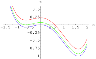
Figure 4: A graph of the potential $v(x)$ for $b=1$, and $z=\{1,0,-1\}$.

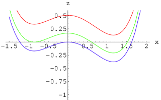
Figure 5: A graph of the potential $v(x)$ for $b=0.3$, and $z=\{1,0,-1\}$.

We employ the same quartic potential used in Ref. BJ , which takes the form

$$v(x)=f(x)-(1+z)f(x_{\rm F})~{},$$ (42)

where

$$f(x)=\frac{x^{4}}{4}-\frac{bx^{3}}{3}-\frac{x^{2}}{2}~{}.$$ (43)

The function $f(x)$ has two negative local minima at $x_{\rm F}$ and $x_{\rm T}$, with $f(x_{\rm F})>f(x_{\rm T})$, and a local maximum at $x=0$. The potential $v(x)$ share these properties.

The adjustable parameter $z$ allows us to tune the false vacuum energy by shifting the entire potential with $v(x_{\rm F})\propto z$. Thus, $z$ plays the role of the shift $V_{\rm F}$ in the previous sections. In particular, the interesting limit $V_{\rm F}\to 0$ corresponds to $z\to 0$. (Note that $f(x_{\rm F})<0$, so $z>0$ corresponds to $V_{\rm F}>0$.)

The parameter $b$, which we take to be strictly positive, controls both the width $x_{\rm T}-x_{\rm F}$ and relative heights of the vacua $v(x_{\rm F})-v(x_{\rm T})$. Figures 4 and 5 show plots of $v(x)$ of $b=1$ and $0.3$, respectively, for various values of $z$.

The radius and time can also be made dimensionless by rescaling by appropriate powers of the mass scales $\mu$ and $M$:

$$r = \frac{\mu^{2}\rho}{M}~{},$$ (44)

$$s = \frac{\mu^{2}t}{M}~{},$$ (45)

$$\epsilon = \frac{M}{\sqrt{3}M_{\rm Pl}}~{}.$$ (46)

We have also defined a dimensionless quantity $\epsilon$ controlling the strength of gravity. For $\epsilon\ll 1$, gravity has a negligible effect on the decay rate, but when $\epsilon$ is of order one, gravity can be important. For example, it can completely suppress the decay of flat space.

Let us rewrite the Euclidean CDL equations (3) and (5) in terms of these dimensionless variables:

$$\ddot{r}=-\epsilon^{2}r\left[\dot{x}^{2}+v(x)\right]~{},$$ (47)

$$\ddot{x}+3\frac{\dot{r}}{r}\dot{x}=v^{\prime}(x)~{},$$ (48)

$$\dot{r}^{2}-1=\epsilon^{2}r^{2}\left[\frac{\dot{x}^{2}}{2}-v(x)\right]~{}.$$ (49)

where an overdot (prime) denotes differentiation with respect to $s$ ($x$).

Using Mathematica, we numerically integrate these equations with initial boundary conditions

$$\dot{r}(0)=1 r(0)=0~{},$$ , (50)

$$\dot{x}(0)=0 x(0)=x_{0}$$ , (51)

to yield functions $r(s)$ and $x(s)$. The initial position $x_{0}$ along with $z$, $b$, and $\epsilon$ form a set of four adjustable parameters on which the solutions depend.

By numerically constructing many solutions, both singular and regular, for a variety of parameters, we will be able to verify the assertions made in sections III and IV. For generic choices of parameters, the numerical integration produces compact singular solutions where the field $x(s)$ inevitably escapes to $\pm\infty$, as explained in Sec. III.3. For regular compact solutions, the unbounded anti-friction as $r\to 0$ makes the numerics difficult to control near the far pole. By tuning $x_{0}$, however, regular solutions can be very well approximated. The range of $r$ over which $x(s)$ can be made to remain near $x_{\rm T}$ or $x_{\rm F}$ before rolling off to $\pm\infty$ is limited only by the tuning of $x_{0}$ and calculational precision.

Noncompact solutions can likewise be approximated by fine-tuning $x_{0}$. In accordance with the arguments of section III, these are necessarily regular one-pass solutions starting at the true vacuum and asymptoting to the false vacuum. As with the approximately regular compact solutions, the inevitable result of imperfect tuning of $x_{0}$ is that $x(s)$ eventually either over- or under-shoots $x_{\rm F}$, leading to a singularity. However, with sufficient tuning, we can obtain a large (in $s$) region where $\dot{r}=1$ and reach a large maximum $r$ before the singularity.

V.2 The decay of nearly flat space

Our first goal is to confirm the result of Sec. III that the decay rate is continuous as $z\to 0$.

As was pointed out in Ref. CDL , for certain potentials a seemingly metastable Minkowski space ($z=0$) can be stabilized by gravitational effects. To exhibit this effect, we tune $\epsilon$ which controls the strength of gravitational corrections. Keeping $b=1$ fixed, we find a critical value of $\epsilon\approx.35$. Below this value, the $z=0$ one-pass solution is noncompact, implying the instanton corresponds to an actual decay of Minkowski space. Above the critical value, the regular one-pass solution is compact at $z=0$ and therefore does not represent decay. A similar transition occurs when varying $b$ for fixed $\epsilon$. For fixed $\epsilon=0.6$, for example, the $z=0$ regular one-pass solutions are compact below $b\approx 0.74$ and noncompact above this value.

We now turn to the question discussed in Sec. III: the behavior of compact, regular one-pass $z>0$ solutions in the limit where $z\to 0$. The asserted continuity of the decay rate translates into different behavior, depending on whether the false vacuuum at $z=0$ is stable or not. We chose $\epsilon=0.6$, $b=.3$ to study the stable case and $\epsilon=0.6$, $b=1$ for the unstable case.

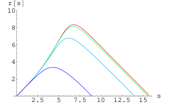
Figure 6: This graph shows a family of one-pass solutions with $b=0.3$, $\epsilon=0.6$, and $z=\{1,0.1,0.01,0\}$. As $z\to 0$, these compact solutions smoothly approach the $z=0$ solution, which for this value of $(b,\epsilon)$ is also compact. The decay of flat space is forbidden. This reproduces the results of BJ

For each case, we probed the $z\to 0$ limit by numerically computing a family of regular single-pass solutions with $z=\{1,0.1,0.01,0\}$. The stable case is shown in figure 6. As expected, the family of compact solutions smoothly approaches the compact $z=0$ solution. This is the behavior anticipated in Sec. III.

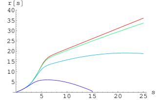
Figure 7: This graph shows a family of one-pass solutions with $b=1$, $\epsilon=0.6$, and $z=\{1,0.1,0.01,0\}$. As $z\to 0$, these compact solutions smoothly approach a noncompact $z=0$ solution. Flat space decays.

In the unstable case, the compact $z>0$ solutions dramatically grow in size as $z\to 0$, as shown in figure 7. For $z\leq 0.1$ we lack the numerical precision to follow the solution all the way to the far pole at $s>30$ because the corresponding dS spheres are growing so large. For $z=0.1$ at least the equator where $\dot{r}=0$ at $s=22$ is still within our computational range. We can clearly infer, though, that as $z\to 0$ the compact instantons are growing so as to reach infinite size in the limit. The $z=0.01$ and $z=0$ solutions are virtually indistinguishable. Again, this supports the behavior anticipated in Sec. III.

In summary, our analytic argument that the decay rate is continuous is borne out by the numerical evidence.

V.3 Plots of the solution space

Our next numerical goal is to verify the broader analysis of the CDL solution space provided in section IV. For fixed $\epsilon=0.6$, we considered the two important cases $b=1$ (flat space decays) and $0.3$ (flat space is stable). For each case, we computed the number of passes for $10^{6}$ solutions with $z\in[-1,9]$ and $x_{0}\in[x_{\rm F},x_{\rm T}]$. The resolution is approximately $\delta x_{0}\sim 10^{-3}$ and $\delta z\sim 10^{-2}$.

The results are shown in figures 8 and 9.

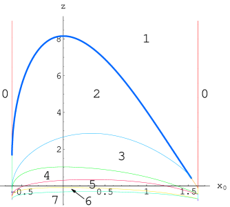
Figure 8: The $(x_{0},z)$ solution space for $b=1$ and $\epsilon=0.6$. This numerical plot reproduces the general features of figure 2. Here, tunneling is allowed at $z=0$. The numbers $0$ to $7$ denote the number of passes for solutions in a given region. The curves at the boundaries between regions are regular solutions. The vertical lines are the trivial solutions at $x_{\rm T}$ and $x_{\rm F}$, and the thick blue line is the single-pass instanton. The Hawking-Moss solution (a vertical line at $x=0$) is hidden by the axis. Features near $x_{\rm T}$ and $x_{\rm F}$ are not well-resolved; see figures 10 and 11

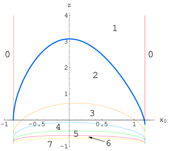
Figure 9: The $(x_{0},z)$ solution space for $b=0.3$ and $\epsilon=0.6$. This numerical plot reproduces the general features of figure 3. Tunneling is not allowed at $z=0$. The numbers $0$ to $7$ denote the number of passes for solutions in a given region, and the curves represent both regular solutions and the boundaries between regions. The vertical lines are the trivial solutions at $x_{\rm T}$ and $x_{\rm F}$, and the thick blue line is the single-pass instanton. Features near $x_{\rm T}$ and $x_{\rm F}$ are not well-resolved; see figures 12 and 13

The number of passes for each region is labeled. The curves demarcating the boundaries between regions with different numbers of passes are the locations of the regular solutions.

To better access features near $x_{\rm F}$ and $x_{\rm T}$, we also ran $10^{5}$ points close to each edge for each value of $b$, with exponentially decreasing step size in $x_{0}$ as the edge was approached. Our resolution was then $\delta\log(x_{0})\sim 10^{-1}$ and $\delta z\sim 10^{-2}$. The magnified left edges of figures 8 and 9 are shown in figures 10 and 12. Likewise, figures 11 and 13 zoom in on the right edge.

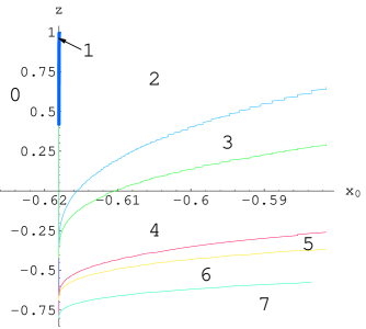
Figure 10: A close-up of the lower-left corner fig. 8 (tunneling allowed at $z=0$), showing the numerically computed $(x_{0},z)$ solution space with $b=1$ and $\epsilon=0.6$. The thick, blue one-pass curve is nearly vertical and is merging with the $x_{\rm F}$ solution. Although we expect that they meet at $z=0$, our limited precision makes them appear to merge at higher $z$.

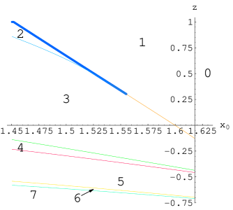
Figure 11: A close-up of the lower right corner of fig. 8 (tunneling allowed at $z=0$) showing the numerically computed $(x_{0},z)$ solution space with $b=1$ and $\epsilon=0.6$. The regular one- (thick, blue line) and two-pass solutions merge as $z$ decreases. Due to our limited precision, they appear to meet at $z=0.3$ rather than at $z=0$ as expected.

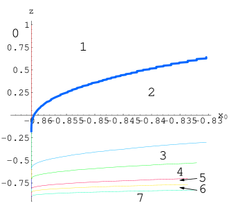
Figure 12: A close-up of the lower left corner fig. 9 (tunneling forbidden at $z=0$) showing the numerically computed $(x_{0},z)$ solution space with $b=0.3$ and $\epsilon=0.6$. One can see that the one-pass regular solution passes through $z=0$ without merging.

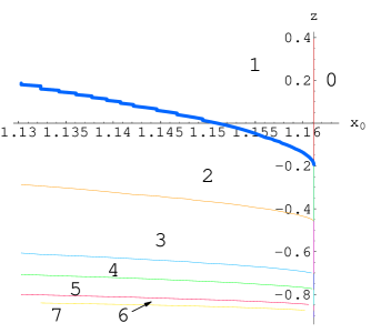
Figure 13: A close-up of the lower right corner fig. 9 (tunneling forbidden at $z=0$) showing the numerically computed $(x_{0},z)$ solution space with $b=0.3$ and $\epsilon=0.6$. Again, one can see that the one-pass regular solution passes through $z=0$ without merging.

V.4 Discussion

A number of important features predicted in figures 2 and 3 are reproduced numerically in figures 8 and 9. As we argued in Sec. III.4, when crossing any regular compact solution, the number of passes should jump by one. This can be seen in figures 8 and 9. It can also be seen that curves representing noncompact solutions separate singular regions whose number of passes differ by as much as seven.

Another notable feature of the $z\to 0$ limit in the unstable case (figure 2) was the merging of solutions as $z\to 0$. As explained in section IV.2, the regular one-and two-pass solutions on the right merge into each other at $z=0$, as do the zero- and one-pass solutions on the left. This was the most obvious feature distinguishing the unstable from the stable diagram (figure 3).

This merger can be roughly made out in our numerical plot for the unstable case, figure 8; and it is notably absent in the stable plot, figure 9. This is best seen in the refined plots for the left and right edge; note how the thick blue line passes through $z=0$ in figures 12 and 13). This supports our arguments in Sec. IV.2.

However, neither figure 8, nor its refinements, figures 10 or 11, are able to show that the merger takes place exactly at $z=0$. The curves become so close together that even at $z=0.1$, a resolution of $\delta x_{0}\sim 10^{-10}$ is insufficient to detect the region between them.

The plots also confirm the estimate in Sec. IV.3 for the number of oscillations for solutions near $x_{0}=0$: The regular solution with the largest number of passes at a given $z>-1$ is given by the largest integer $n$ satisfying Eq. (30), which in dimensionless variables is

$$n(n+3)<\frac{|v^{\prime\prime}(0)|}{\epsilon^{2}v(0)}~{}.$$ (52)

For example, in the $b=1$ case, at $z=1$ the right-hand side of Eq. (52) is $18.3$ which yields $n=3$. From figure 8, we can see the curve of regular three-pass solutions crosses the origin just above $z=1$. Below it, in particular at $z=1$ near $x=0$, are singular three-pass solutions.

Confirming a prediction from Sec. IV.4, the regular solution curves begin to pile up when $z\to-1$, in both figure 8 and figure 9. Ultimately, the resolution is insufficient to detect every transition between constant-pass regions. As $z\to-1$ the number of oscillations increases rapidly, the amplitude decreases, and the size of the solutions grow very large, $s\gg 1$. For example, when $b=1$ , $z=0.99$, and $|x_{0}-x_{\rm T}|=10^{-5}$, $x(s)$ oscillates for so long around the Hawking-Moss solution, that the numerical precision is insufficient to follow the solution back to $r=0$, and instead errors build up and lead to a singularity at $s\sim 130$.

The plots also connect with the discussion in Sec. IV. For $z<0$, the regular solutions appear to merge in pairs before reaching $x_{\rm F}$ or $x_{\rm T}$. However, we can resolve the two curves, and, when we zoom in on the edges by plotting figures 10 and 12 logarithmically in $x_{0}-x_{\rm F}$ in or figures 11 and 13 logarithmically in $x_{\rm T}-x_{0}$, we can see the curves reach $x_{\rm F}$ or $x_{\rm T}$ at separate points.

- (1) R. Bousso and J. Polchinski: Quantization of four-form fluxes and dynamical neutralization of the cosmological constant. JHEP 06, 006 (2000), hep-th/0004134.
- (2) M. R. Douglas: The statistics of string / M theory vacua. JHEP 05, 046 (2003), hep-th/0303194.
- (3) F. Denef and M. R. Douglas: Distributions of flux vacua. JHEP 05, 072 (2004), hep-th/0404116.
- (4) S. Kachru, R. Kallosh, A. Linde and S. P. Trivedi: De Sitter vacua in string theory. Phys. Rev. D 68, 046005 (2003), hep-th/0301240.
- (5) K. Dasgupta, G. Rajesh and S. Sethi: M theory, orientifolds and g-flux. JHEP 08, 023 (1999), hep-th/9908088.
- (6) S. B. Giddings, S. Kachru and J. Polchinski: Hierarchies from fluxes in string compactifications. Phys. Rev. D 66, 106006 (2002), hep-th/0105097.
- (7) F. Denef, M. R. Douglas, B. Florea, A. Grassi and S. Kachru: Fixing all moduli in a simple F-theory compactification (2005), hep-th/0503124.
- (8) F. Denef, M. R. Douglas and B. Florea: Building a better racetrack. JHEP 06, 034 (2004), hep-th/0404257.
- (9) J. P. Conlon, F. Quevedo and K. Suruliz: Large-volume flux compactifications: Moduli spectrum and D3/D7 soft supersymmetry breaking. JHEP 08, 007 (2005), hep-th/0505076.
- (10) P. Berglund and P. Mayr: Non-perturbative superpotentials in F-theory and string duality (2005), hep-th/0504058.
- (11) V. Balasubramanian, P. Berglund, J. P. Conlon and F. Quevedo: Systematics of moduli stabilisation in Calabi-Yau flux compactifications. JHEP 03, 007 (2005), hep-th/0502058.
- (12) A. Saltman and E. Silverstein: A new handle on de Sitter compactifications (2004), hep-th/0411271.
- (13) A. Saltman and E. Silverstein: The scaling of the no-scale potential and de Sitter model building. JHEP 11, 066 (2004), hep-th/0402135.
- (14) A. Maloney, E. Silverstein and A. Strominger: De Sitter space in noncritical string theory (2002), hep-th/0205316.
- (15) B. S. Acharya: A moduli fixing mechanism in M theory (2002), hep-th/0212294.
- (16) B. de Carlos, A. Lukas and S. Morris: Non-perturbative vacua for M-theory on G(2) manifolds. JHEP 12, 018 (2004), hep-th/0409255.
- (17) G. Curio, A. Krause and D. Lust: Moduli stabilization in the heterotic / IIB discretuum (2005), hep-th/0502168.
- (18) S. Gurrieri, A. Lukas and A. Micu: Heterotic on half-flat. Phys. Rev. D 70, 126009 (2004), hep-th/0408121.
- (19) K. Becker, M. Becker, P. S. Green, K. Dasgupta and E. Sharpe: Compactifications of heterotic strings on non-Kaehler complex manifolds. II. Nucl. Phys. B678, 19 (2004), hep-th/0310058.
- (20) M. Becker, G. Curio and A. Krause: De Sitter vacua from heterotic M-theory. Nucl. Phys. B693, 223 (2004), hep-th/0403027.
- (21) R. Brustein and S. P. de Alwis: Moduli potentials in string compactifications with fluxes: Mapping the discretuum. Phys. Rev. D 69, 126006 (2004), hep-th/0402088.
- (22) S. Gukov, S. Kachru, X. Liu and L. McAllister: Heterotic moduli stabilization with fractional Chern-Simons invariants. Phys. Rev. D 69, 086008 (2004), hep-th/0310159.
- (23) E. I. Buchbinder and B. A. Ovrut: Vacuum stability in heterotic M-theory. Phys. Rev. D 69, 086010 (2004), hep-th/0310112.
- (24) O. DeWolfe, A. Giryavets, S. Kachru and W. Taylor: Type IIA moduli stabilization. JHEP 07, 066 (2005), hep-th/0505160.
- (25) L. Susskind: The anthropic landscape of string theory (2003), hep-th/0302219.
- (26) A. Vilenkin: Probabilities in the landscape (2006), hep-th/0602264.
- (27) A. Linde, D. Linde and A. Mezhlumian: From the big bang theory to the theory of a stationary universe. Phys. Rev. D 49, 1783 (1994), gr-qc/9306035.
- (28) J. Garriga, D. Schwartz-Perlov, A. Vilenkin and S. Winitzki: Probabilities in the inflationary multiverse. JCAP 0601, 017 (2006), hep-th/0509184.
- (29) R. Easther, E. A. Lim and M. R. Martin: Counting pockets with world lines in eternal inflation (2005), astro-ph/0511233.
- (30) J. Garriga and A. Vilenkin: A prescription for probabilities in eternal inflation. Phys. Rev. D 64, 023507 (2001), gr-qc/0102090.
- (31) R. Bousso and I.-S. Yang: to appear.
- (32) L. Susskind, L. Thorlacius and J. Uglum: The stretched horizon and black hole complementarity. Phys. Rev. D 48, 3743 (1993), hep-th/9306069.
- (33) R. Bousso: Holography in general space-times. JHEP 06, 028 (1999), hep-th/9906022.
- (34) W. Fischler: Taking de Sitter seriously. Talk given at Role of Scaling Laws in Physics and Biology (Celebrating the 60th Birthday of Geoffrey West), Santa Fe, Dec. 2000.
- (35) T. Banks: Cosmological breaking of supersymmetry or little Lambda goes back to the future II (2000), hep-th/0007146.
- (36) R. Bousso: Positive vacuum energy and the N-bound. JHEP 11, 038 (2000), hep-th/0010252.
- (37) R. Bousso: Bekenstein bounds in de Sitter and flat space. JHEP 04, 035 (2001), hep-th/0012052.
- (38) T. Banks and W. Fischler: M-theory observables for cosmological space-times (2001), hep-th/0102077.
- (39) L. Dyson, M. Kleban and L. Susskind: Disturbing implications of a cosmological constant. JHEP 10, 011 (2002), hep-th/0208013.
- (40) R. Bousso: A covariant entropy conjecture. JHEP 07, 004 (1999), hep-th/9905177.
- (41) B. Freivogel and L. Susskind: A framework for the landscape (2004), hep-th/0408133.
- (42) T. Banks: Landskepticism: or why effective potentials don’t count string models (2004), hep-th/0412129.
- (43) R. Bousso: Cosmology and the S-matrix. Phys. Rev. D 71, 064024 (2005), hep-th/0412197.
- (44) R. Bousso and B. Freivogel: Asymptotic states of the bounce geometry (2005), hep-th/0511084.
- (45) A. Vilenkin: Unambiguous probabilities in an eternally inflating universe. Phys. Rev. Lett. 81, 5501 (1998), hep-th/9806185.
- (46) T. Banks and M. Johnson: Regulating eternal inflation (2005), hep-th/0512141.
- (47) F. Denef and M. R. Douglas: Computational complexity of the landscape. I (2006), hep-th/0602072.
- (48) S. Coleman and F. D. Luccia: Gravitational effects on and of vacuum decay. Phys. Rev. D 21, 3305 (1980).
- (49) S. Coleman: The fate of the false vacuum. 1. Semiclassical theory. Phys. Rev. D 15, 2929 (1977).
- (50) C. G. Callan and S. Coleman: The fate of the false vacuum. 2. First quantum corrections. Phys. Rev. D 16, 1762 (1977).
- (51) S. W. Hawking and I. G. Moss: Fluctuations in the inflationary universe. Nucl. Phys. B224, 180 (1983).
- (52) A. Linde: Quantum creation of an open inflationary universe. Phys. Rev. D 58, 083514 (1998), gr-qc/9802038.
- (53) J. C. Hackworth and E. J. Weinberg: Oscillating bounce solutions and vacuum tunneling in de Sitter spacetime. Phys. Rev. D 71, 044014 (2005), hep-th/0410142.
- (54) R. Bousso and A. Linde: Quantum creation of a universe with : Singular and non-singular instantons. Phys. Rev. D 58, 083503 (1998), gr-qc/9803068.
- (55) S. Gratton and N. Turok: Homogeneous modes of cosmological instantons. Phys. Rev. D 63, 123514 (2001), hep-th/0008235.