March 14, 2006 xxx

EFI-06-03

Toward the End of Time

Emil J. Martinec, Daniel Robbins and Savdeep Sethi

Enrico Fermi Institute, University of Chicago, Chicago, IL 60637, USA

The null-brane space-time provides a simple model of a big crunch/big bang singularity. A non-perturbative definition of M-theory on this space-time was recently provided using matrix theory. We derive the fermion couplings for this matrix model and study the leading quantum effects. These effects include particle production and a time-dependent potential. Our results suggest that as the null-brane develops a big crunch singularity, the usual notion of space-time is replaced by an interacting gluon phase. This gluon phase appears to constitute the end of our conventional picture of space and time.

1 Introduction

One of the major gaps in our understanding of string theory is how it resolves space-like singularities. A related issue is how to formulate dynamics in time-dependent backgrounds non-perturbatively. The various gauge/gravity correspondences subsume a resolution of space-like singularities when they are localized inside black hole event horizons. Implicitly, there must be encoded the experience of a freely falling observer who sees a time-dependent background culminating in a space-like singularity. One might then wonder whether there is a regularization of cosmological singularities via gauge theory.

Recently, some examples of such regularizations via gauge theory have been concretely described in [1, 2, 3, 4, 5, 6, 7, 8, 9, 10, 11, 12, 13, 14]. These holographic models, based on matrix theory [15], appear to contain the right degrees of freedom to describe physics at large blue shifts. In each case the semi-classical picture of the space-time singularity is replaced by a gluon phase. We will find further evidence for this picture in this work. Quantum effects in such models are quite fascinating have been examined recently in [16, 17].

Our goal is to develop this matrix approach when applied to M-theory in the particular background known as the null-brane space-time [18, 19]. The matrix model for this space-time was introduced recently in [20]. The null-brane is constructed using a particularly simple way of generating time dependence: namely, by orbifolding Minkowski space by a discrete subgroup of the Poincaré group. This can yield a time-dependent background. For appropriate choices of orbifold group generators, this background can be singular.

The null-brane is actually a non-singular solution of M-theory defined by choosing an $\mathbb{R}^{1,3}$ subspace of $\mathbb{R}^{1,10}$ with coordinates

$$x^{\pm}=\frac{1}{\sqrt{2}}(x^{0}\pm x^{1}),\,x,\,z,$$

and the usual flat metric $ds^{2}=-2dx^{+}dx^{-}+dx^{2}+dz^{2}$. We act on these coordinates by an element of the 4-dimensional Poincaré group

$$g=\exp(2\pi iK);\quad K=\frac{\lambda}{\sqrt{2}}(J^{0x}+J^{1x})+LP^{z},$$ (1)

where $L$ has dimensions of length. Under this action which depends on $(\lambda,L)$,

$$X=\left(\begin{array}[]{c}x^{+}\\ x^{-}\\ x\\ z\\ \end{array}\right)\ \rightarrow\quad g\cdot X=\left(\begin{array}[]{c}x^{+}\\ x^{-}+2\pi\lambda x+2\pi^{2}\lambda^{2}x^{+}\\ x+2\pi\lambda x^{+}\\ z+2\pi L\\ \end{array}\right).$$ (2)

When $L$ goes to zero, the geometry has a null singularity at $x^{+}=0$. This space-time is depicted in figure 1.

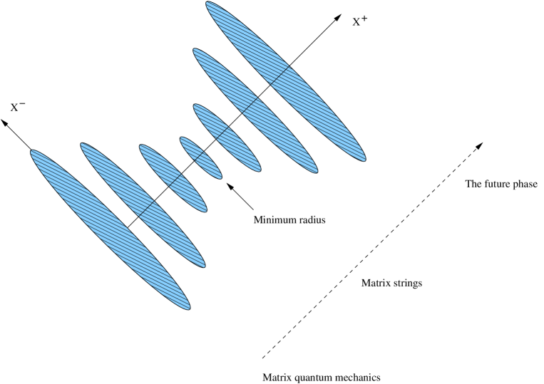
Figure 1: The circle radius shrinks to a minimum size $L$ at $x^{+}=0$.

For $L$ large compared to the Planck scale, this is simply a smooth time-dependent background of M-theory or string theory with a well-defined S-matrix. String perturbation theory on this background has been studied in [21, 22, 23] while the semi-classical stability of this space-time has been examined in [24, 25]. Not surprisingly, string perturbation theory breaks down as $L\rightarrow 0$. Holographic descriptions of string cosmologies, in the spirit of AdS/CFT, have been studied in [26, 27, 28]. In the case of the null-brane, these descriptions involve space-time non-commutative Yang-Mills theories.

By contrast, the matrix description is obtained by performing an additional light-like compactification $x^{-}\sim x^{-}+2\pi R$ which commutes with the orbifold identification $(\ref{quotgroup})$. This results in a discrete light-cone quantized description of the theory. In close analogy to the flat space case [29], there is a decoupling limit [20] that reduces the matrix model to the low-energy dynamics of D0-branes moving in the orbifold (2).

The matrix theory description can also be thought of as viewing the system from the perspective of a highly boosted frame. It does not directly describe the space-time vacuum, but rather describes objects in space-time that carry large $p^{+}$, and therefore preserve at most one-half of the supersymmetries. In the case of the null-brane, the one-half of the supersymmetries preserved by the orbifold identification are incompatible with the one-half of the supersymmetries preserved by boosting along the light-cone direction. Thus the null-brane matrix model preserves no supersymmetry. We will see this explicitly when we evaluate the one-loop effective potential of the model, and compute the amplitude for particle production.

We can understand the dynamics of a D0-brane in this orbifold background from the perspective of the covering space of the orbifold group action $(\ref{quotgroup})$. On the covering space, we see a D0-brane together with an array of boosted images constrained to move in a manner invariant under the identification $(\ref{quotgroup})$. The interactions between the image branes arise from the usual velocity-dependent forces between D0-branes.

Semi-classically, when the brane and enough of its images are contained within their Schwarzschild radius, a black hole forms. For finite $L$, the black hole eventually decays and we can compute a conventional S-matrix. However, as $L$ becomes small, this black hole becomes larger eventually filling all of space [25]. We will find a quite different picture of this process from the matrix model which, in particular, includes degrees of freedom not seen in the semi-classical picture.

T-dualization of this system of D0-branes along the $z$ direction circle yields a D1-brane matrix string theory description. The evolution from matrix quantum mechanics to matrix strings near the singularity is also depicted in figure 1. Physics near the singularity is controlled by $1+1$-dimensional field theory dynamics rather than quantum mechanics. In principle, the future phase is a return to matrix quantum mechanics as the z circle becomes large again (and the T-dual field theory circle becomes small).

However, strong quantum effects near the singularity can drastically alter the future description. Determining these quantum effects at one-loop in the matrix model is our primary task. We will find that a potential is generated in the matrix model which turns off at early and late times. This supports the consistency of the model since we need exact flat directions in the far past and future to recover a semi-classical picture of space-time.

The potential tends to attract gravitons more and more strongly as they approach $x^{+}=0$ and as we tune $L\rightarrow 0$. This effective potential as a function of the impact parameter for two gravitons is displayed in figure 2. As the gravitons approach each other, the off-diagonal matrix degrees of freedom become lighter and our notion of space-time becomes fuzzy and is eventually replaced by matrix dynamics. At this level of approximation, it appears that there is no escape from this gluon phase as $L\rightarrow 0$.

Figure 2: The potential given in $(\ref{finalpot})$ as a function of impact parameter with various choices of $L$. The smaller $L$, the deeper the potential well. The choice of parameters is described in section 3.4.

The attraction of gravitons as $x^{+}$ and $L$ go to zero is a reflection of their interaction with one another’s images under the orbifold group. In fact, even a single graviton interacts with its own images and can generate a spacelike singularity at the null-brane neck at $x^{+}=0$; even if the vacuum does not evolve to a singularity, excited states can do so. The null-brane matrix model describes objects (such as gravitons) carrying longitudinal momentum in the null-brane background, rather than being a description of the null-brane vacuum directly. Thus even the ground state of the matrix model can evolve to a singularity when $L$ is small enough. This property is related to the lack of supersymmetry of the null-brane matrix model.

The formation of such singularities by excitations on the null-brane was analyzed by Horowitz and Polchinski from the point of view of the dual gravitational theory in [25]. They argued that a spacelike singularity will form in the null-brane orbifold whenever the gravitational radius of excitations exceeds the proper size $L$ of the null-brane neck at $x^{+}=0$. For $d>4$ noncompact spatial dimensions, the singularity that results is a finite-sized black hole; outside the black hole there is no big crunch singularity. The gravitational radius of the black hole is

$$r_{0}=\Bigl{(}\frac{G_{\!N}\,p^{+}}{L^{2}}\Bigr{)}^{\frac{1}{d-4}}$$ (3)

in terms of the effective $d+1$ dimensional Newton constant $G_{N}$ and momentum $p^{+}$ of the initial excitation. In particular, the size of the black hole grows to infinity as $L\to 0$. For $d=4$, no black hole forms for large $L$, and an infinite mass black hole forms for small $L$. For $d<4$, a spacelike singularity of infinite extent always forms.

The interesting regime of $d<4$ is outside the reach of matrix theory. Matrix theory constructions describe gravity in terms of a dual field theory for $d>5$, and a dual “little string theory” for $d=5$; there are no constructions for $d<5$ (because the growth of the density of states is too rapid to be described by a field theory or nongravitational string theory). Thus, for finite $L$, matrix theory is only capable of describing the regime where the outcome of objects falling through the neck of the null-brane is a finite-sized black hole. The size of that black hole grows to infinity as $L/\ell_{p}$ goes to zero. One might view the matrix theory as a description of the cosmological horizon that forms in this limit.

Black holes are well-approximated in matrix theory at finite $N$ provided their entropy is less than $N$ [31, 32, 33]. Therefore, the growing size of the final state black hole with decreasing $L$ puts a lower bound on $N$

$$N_{\rm min}\sim\Bigl{(}\frac{\ell_{p}^{3}p^{+}}{L^{2}}\Bigr{)}^{\frac{d-1}{d-4}}$$ (4)

in order to have the matrix model approximate well the bulk gravitational physics. A conservative order of limits sends $N\to\infty$ first, then $L\to 0$ to achieve a cosmological singularity. The dynamics may sensitively depend on this order of limits, however an intriguing possibility is that one could obtain a useful picture of the cosmological singularity by taking $L\to 0$ for finite $N$ and then subsequently the large $N$ limit. The $L\to 0$ limit of the finite $N$ theory accesses the perturbative regime of the gauge theory; if this order of limits is germane, the cosmological singularity devolves to a kind of free gluon phase. If on the other hand the order of limits does not commute, one will need to contend with the strong coupling, large $N$ physics of the gauge theory; still, the matrix model seems to provide a resolution of the cosmological singularity.

This picture of the null brane is very much in accord with the model studied in [1, 17] in which time begins in a free gluon phase. While our understanding of the gluon phase (free or otherwise) in the null-brane is still quite preliminary with much to be understood, it is exciting that the matrix model appears to be a complete description containing all the ingredients necessary for understanding the fate of the S-matrix and, indeed, the fate of space and time.

2 The Matrix Action

Our first task is to determine the complete action for the matrix description of M-theory on the null-brane. The bosonic couplings were determined in [20], but we also require the fermion couplings to compute quantum corrections.

2.1 Parameters, scales and sectors

It is important to keep track of the scales appearing in this system. The space-time physics depends on the matrix theory parameters $(\ell_{p},R)$ as well as the orbifold parameters $(L,\lambda)$. The former are related to string theory parameters $(\ell_{s},g_{s})$ via

$$\ell_{p}=g_{s}^{1/3}\ell_{s},\quad\qquad R=g_{s}\ell_{s}.$$ (5)

We will express the matrix action in terms of string parameters and set $\ell_{s}=1$ for simplicity. The bosonic couplings in the matrix model describing M-theory on the null-brane with $p^{+}=N/R$ are given by a $1+1$-dimensional $U(N)$ gauge theory with action [20]

$$S = \frac{1}{g_{s}}\int d\tau d\sigma\,{\rm Tr\,}\left(\vphantom{\frac{i\tau}{\sqrt{2}}}(D_{0}x^{i})^{2}+(D_{0}x)^{2}-L^{2}(D_{1}x^{i})^{2}-L^{2}(D_{1}x)^{2}-\sqrt{2}\lambda(x-\tau D_{0}x)F\right.$$ (6)

$$\hskip 85.35826pt\left.+(L^{2}+\frac{1}{2}\lambda^{2}\tau^{2})F^{2}+{1\over 2}\left[x^{i},x^{j}\right]^{2}+(\left[x,x^{i}\right]+{i\tau\lambda\over\sqrt{2}}D_{1}x^{i})^{2}\right),$$

where $0\leq\sigma\leq 2\pi$. Here $\tau$ can be identified with the coordinate $x^{+}$ and $\sigma$ is a coordinate T-dual to $z$.

There are $7$ scalar fields $x^{i}$ rotated by an $SO(7)$ symmetry. There is an additional scalar field $x$ distinguished by the orbifold identification $(\ref{quotgroup})$ and a $U(N)$ gauge field with field strength $F$. Each of these adjoint-valued fields has canonical mass dimension $1$ while $\sigma,\tau$ and $L$ have length dimension $1$. These are the natural dimension assignments from the perspective of gauge theory. Lastly, we note that as $\lambda\rightarrow 0$, we recover standard matrix string theory [34, 35, 36].

The singularity that develops in space-time as $L\rightarrow 0$ is reflected classically in the matrix model by the appearance of a new flat directions at $\tau=0$. These flat directions correspond to $\sigma$ fluctuations of the $x^{i}$ fields which are suppressed by the couplings,

$$(L^{2}+\frac{1}{2}\lambda^{2}\tau^{2})(D_{1}x^{i})^{2},$$ (7)

which vanish at $L=\tau=0$. We will examine how this classical picture is modified quantum mechanically.

This model can also be extended to describe string theory on the null-brane, or more generally M-theory on products of tori with the null-brane. This extension is straightforward and involves promoting some of the $x^{i}$ to gauge-fields while increasing the dimension of the field theory in the usual way [37]

$$x^{i}\rightarrow A^{i}.$$ (8)

These extensions are already interesting for the case of string theory on the null-brane. Type IIA on the null-brane involves an extension of type IIB matrix string theory [38, 35] in which time-dependent non-perturbative field theory effects should play an important role. On the other hand, type IIB on the null-brane involves a $3+1$-dimensional time-dependent gauge theory generalizing [39, 40]. The action of S-duality in this theory should be quite fascinating. We will not pursue these directions here.

Lastly we note that the M-theory on the null-brane has superselection sectors specified by the quantized amount of graviton momentum on the z circle. This circle is large at infinity so these excitations are finite energy. Each sector with non-zero momentum can be studied in the matrix model by analyzing the quantum dynamics expanded around a classical background with non-zero electric flux.

2.2 Decoupling revisited and the large $N$ scaling

The decoupling limit for the null-brane matrix model can be understood along the lines of the original argument given in [15]. Let us return to the orbifold perspective where we consider an array of D0-branes to make the connection between the arguments and determine how to take the large $N$ limit.

The D0-brane action in string units has the schematic form

$${\cal S}=\frac{1}{g_{s}\ell_{s}}\int\!dt\,\Bigl{(}(\partial_{t}x)^{2}+[x,x]^{2}/\ell_{s}^{4}+{\rm fermions}\Bigr{)}\ .$$ (9)

The matrix theory limit sends the dimensionless parameter $g_{s}$ to zero, holding fixed the dimensionless quantities

$$\hat{t}=g_{s}^{1/3}t/\ell_{s}=Rt/\ell_{p}^{2},\quad\qquad\hat{x}=g_{s}^{-1/3}x/\ell_{s}=x/\ell_{p}.$$ (10)

The action expressed in terms of these parameters refers only to quantities in the resulting eleven-dimensional theory

$${\cal S}=\int\!d\hat{t}\,\Bigl{[}\Bigl{(}\frac{\partial\hat{x}}{\partial\hat{t}}\Bigr{)}^{2}+[\hat{x},\hat{x}]+{\rm fermions}\Bigr{]}\ .$$ (11)

At these scales the interactions are of unit strength.

We now come to the issue of scaling the parameters $(L,\lambda)$ of the null-brane orbifold. First of all, we should hold fixed $L/\ell_{p}$, the size of the neck in the geometry at $\tau=0$ in eleven-dimensional Planck units. The scaling of $\lambda$ is can be understood from the underlying D0-brane picture which is related to the 1+1 QFT appearing in (6) as a T-dual representation.

In the D0-brane picture, one has groups of D0-branes in relative motion on different fundamental domains of the covering space of the orbifold. Strings stretching between image branes are represented by the Fourier modes of the 1+1 field theory. The D0-brane representation is, however, useful for understanding the matrix theory scaling limit of the null brane orbifold. The kinetic energy of relative D0-brane motion is excess energy above the BPS threshold

$$E_{\rm YM}=E-N/R=\sqrt{(N/R)^{2}+\vec{p}^{2}}-N/R=\frac{\vec{p}^{2}}{2N/R}+\dots$$ (12)

where the subleading terms in the last expression vanish in the scaling limit. The time scale (10) means the energy in the D0-brane dynamics should scale in order to keep $E_{\rm YM}\ell_{s}g_{s}^{-1/3}$ fixed. Equivalently, we are holding fixed

$$\ell_{p}^{2}\vec{p}^{2}=E_{\rm YM}\cdot 2N(\ell_{p}^{2}/R)\ .$$ (13)

Now, D0-branes on neighboring images of the covering space have relative kinetic energy

$$\ell_{p}^{2}(p-g\cdot p)^{2}=(2\pi\lambda\ell_{p}/R)^{2}\ .$$ (14)

In order to hold this quantity fixed, $\lambda$ must scale as $\lambda\sim g_{s}^{2/3}$. This is the scaling limit proposed in [20]. In particular, standard matrix theory arguments for the decoupling of both higher string modes and ten-dimensional gravitational physics may be directly carried over to the null-brane matrix model.

More precisely, decoupling holds as long as one takes the scaling limit first holding fixed

$$L/\ell_{p},\quad\ell_{p}^{2}E_{\rm YM}/R,\quad\lambda/g_{s}^{2/3},$$ (15)

for fixed $N$. One can then contemplate further taking $L/\ell_{p}$ to zero, or $N$ to infinity, in various combinations.

Consider now the large $N$ limit. In order to hold the invariant mass (13) fixed as we scale $N$, the Yang-Mills energy $E_{\rm YM}$ should scale as $1/N$. Since there are $N$ D0-branes, the kinetic energy $v^{2}/R$ of each must scale as $1/N^{2}$, or $v\sim 1/N$ (i.e. the velocity slows canonically as one boosts the frame by dialing $N$). The relative velocity of D0-branes related by $g^{n}$ is $2\pi n\lambda$; thus $\lambda\sim 1/N$.

2.3 Fermion couplings from the quotient action

To derive the fermion couplings, we can use the orbifold description of the null-brane. We will begin by studying the Euclidean instanton problem and then extend the result to D0-branes moving on the null-brane. The Euclidean instanton problem was also studied in [41].

The supersymmetric instanton action in flat space is given by

$$S=-{\rm Tr\,}\left(\frac{1}{4}\left[X_{\mu},X_{\nu}\right]\left[X^{\mu},X^{\nu}\right]-\bar{\Theta}\gamma_{\mu}\left[X^{\mu},\Theta\right]\right),$$ (16)

where $X^{\mu}$ are bosons with $\mu=0,\ldots,9$. The fermion, $\Theta$, is the dimensional reduction of a Majorana-Weyl spinor in ten dimensions. Both $X^{\mu}$ and $\Theta$ are in the adjoint representation of the gauge group. We will take the gauge group to be $U(N)$. For the moment, we will take all fields to be dimensionless.

We can express the action of the null-brane quotient group on the $X^{\mu}$ in the following way

$$X\,\rightarrow\,\exp(\omega)X+a$$ (17)

where

$$\omega^{\mu}\vphantom{\omega}_{\nu}=\eta^{\mu\rho}\omega_{\rho\nu},$$ (18)

and

$$\omega_{x+}=-\omega_{+x}=2\pi\lambda,\qquad a^{z}=2\pi L,$$ (19)

with all other components vanishing.

The actions on the fermions can then be easily computed. The translations have no effect on a spinor representation, while the Lorentz transformation acts via

$$\Theta\,\rightarrow\,\exp\left(\frac{1}{4}\omega_{\mu\nu}\gamma^{\mu\nu}\right)\Theta=\left(1-\pi\lambda\gamma^{+x}\right)\Theta.$$ (20)

Note that half of the fermions, those that are annihilated by $\gamma^{+}$, are invariant under the quotient action. This is equivalent to the statement that the background preserves one-half of the supersymmetries.

2.3.1 Instantons on the quotient space

We are now ready to study instantons on the quotient. This should really be viewed as a formal exercise on route to determining couplings for dynamical D-branes on the null-brane. So we view $X^{\mu}$ and $\psi$ as infinite matrices satisfying the constraints imposed by invariance under the quotient action

$$X^{+,i}_{m+k,n+k} = X^{+,i}_{mn},$$

$$X_{m+k,n+k} = X_{mn}+2\pi k\lambda X^{+}_{mn},$$

$$X^{-}_{m+k,n+k} = X^{-}_{mn}+2\pi k\lambda X_{mn}+2\pi^{2}k^{2}\lambda^{2}X^{+}_{mn},$$ (21)

$$Z_{m+k,n+k} = Z_{mn}+2\pi kL\delta_{mn},$$

$$\Theta_{m+k,n+k} = \left(1-\pi k\lambda\gamma^{+x}\right)\Theta_{mn}.$$

As usual, we Fourier transform this system (see [20] for this procedure applied to the bosons in this case). The matrix $\Theta_{mn}$ is replaced by the operator

$$\Theta(\sigma,\sigma^{\prime})=\sum_{m,n}e^{i(n\sigma^{\prime}-m\sigma)}\Theta_{mn}=\left[\theta(\sigma)-\frac{i\lambda}{2}\gamma^{+x}\theta(\sigma)\partial_{\sigma}\right]\,\delta(\sigma-\sigma^{\prime})$$ (22)

where $0\leq\sigma\leq 2\pi$. The function $\theta(\sigma)$ appearing in $(\ref{Fourier})$ is not Hermitian but this can be corrected by defining

$$\tilde{\theta}=\theta+\frac{i\lambda}{4}\gamma^{+x}\theta^{\prime},$$ (23)

where the prime denotes a $\sigma$-derivative. Expressed in terms of $\tilde{\theta}$, the operator $\Theta$ is Hermitian:

$$\Theta=\tilde{\theta}-\frac{i\lambda}{4}\gamma^{+x}\tilde{\theta}^{\prime}-\frac{i\lambda}{2}\gamma^{+x}\tilde{\theta}\partial_{\sigma}.$$ (24)

Under a gauge transformation, $\tilde{\theta}$ transforms according to the rule

$$\tilde{\theta}\rightarrow u\tilde{\theta}u^{\dagger}+\frac{i\lambda}{4}\gamma^{+x}\left(u^{\prime}\tilde{\theta}u^{\dagger}-u\tilde{\theta}u^{{\dagger}\prime}\right)$$ (25)

where $u(\sigma)$ is an element of $U(N)$ for the case of $N$ instantons. This is an unconventional gauge transformation rule. With $L\neq 0$, we can define a natural gauge covariant fermion,

$$\hat{\theta}=\tilde{\theta}+\frac{\lambda}{4L}\gamma^{+x}\left\{z,\tilde{\theta}\right\}.$$ (26)

If we also define the covariant derivative, $D_{1}=\partial_{\sigma}-iL^{-1}z$, then we see that

$$\Theta=\hat{\theta}-\frac{i\lambda}{4}\gamma^{+x}\left\{D_{1},\hat{\theta}\right\}$$ (27)

which is manifestly Hermitian and covariant.

We can combine this expression with the analogous operator expressions for the bosons found in [20]

$$X^{+,i}=x^{+,i},$$

$$X=\hat{x}+\frac{i\lambda}{2}\left\{x^{+},D_{1}\right\},$$

$$X^{-}={\hat{x}}^{-}+\frac{i\lambda}{2}\left\{\hat{x},D_{1}\right\}-\frac{\lambda^{2}}{2}D_{1}\cdot x^{+}\cdot D_{1},$$

$$Z=iLD_{1},$$ (28)

to compute the Yukawa coupling appearing in $(\ref{instaction})$

$${\rm Tr\,}\left(\bar{\Theta}\gamma_{\mu}\left[X^{\mu},\Theta\right]\right) = {1\over 2\pi}\int d\sigma\,{\rm Tr\,}\left(\vphantom{\frac{\lambda^{2}}{8}}iL\bar{\theta}\gamma^{z}D_{1}\theta+\bar{\theta}\left[-\gamma^{-}x^{+}-\gamma^{+}{\hat{x}}^{-}+\gamma^{x}\hat{x}+\gamma^{i}x^{i},\theta\right]\right.$$ (29)

$$\left.+\frac{i\lambda}{4}\left(\bar{\theta}\gamma^{+-x}\left\{\theta,D_{1}x^{+}\right\}+\bar{\theta}\gamma^{+xi}\left\{\theta,D_{1}x^{i}\right\}-D_{1}\bar{\theta}\gamma^{x}\left\{\theta,x^{+}\right\}\right.\right.$$

$$\left.\left.+\bar{\theta}\gamma^{x}\left\{D_{1}\theta,x^{+}\right\}+D_{1}\bar{\theta}\gamma^{+}\left\{\theta,\hat{x}\right\}-\bar{\theta}\gamma^{+}\left\{D_{1}\theta,\hat{x}\right\}\right)\right.$$

$$\left.+\frac{\lambda^{2}}{8}\left(D_{1}\bar{\theta}\gamma^{+}\left[D_{1}\theta,x^{+}\right]-D_{1}\bar{\theta}\gamma^{+}\left[\theta,D_{1}x^{+}\right]\right.\right.$$

$$\left.\left.-\bar{\theta}\gamma^{+}\left[D_{1}\theta,D_{1}x^{+}\right]\right)\vphantom{\frac{\lambda^{2}}{8}}\right).$$

We have dropped the hats on each $\theta$ appearing in $(\ref{yukawa})$ to avoid notational clutter. Some of the terms above are not manifestly Hermitian but this is not problematic since they can be made Hermitian by adding total derivatives. We will see momentarily that those terms vanish in the decoupling limit.

In the abelian case where $N=1$, this Yukawa simplifies to the form

$$\bar{\Theta}\gamma_{\mu}\left[X^{\mu},\Theta\right] = {1\over 2\pi}\int d\sigma\left(iL\bar{\theta}\gamma^{z}D_{1}\theta+\frac{i\lambda}{2}\left(\bar{\theta}\gamma^{+-x}\theta D_{1}x^{+}+\bar{\theta}\gamma^{+xi}\theta D_{1}x^{i}\right.\right.$$ (30)

$$\left.\vphantom{\frac{i\lambda}{2}}\left.+2x^{+}\bar{\theta}\gamma^{x}D_{1}\theta-2x\bar{\theta}\gamma^{+}D_{1}\theta\right)\right).$$

It is worth noting that only couplings involving two fermions appear in the action. No four fermion couplings are generated. This is natural since since we are considering a smooth quotient of flat space which has vanishing curvatures.

2.3.2 The extension to quantum mechanics

Let us recall the procedure which we followed in the boson sector to go from the instanton action to the Lorentzian theory describing D0-branes. We let our ten matrices $X^{\mu}_{mn}$ be functions of $\tau$ and we added a kinetic term $D_{0}X_{\mu}D_{0}X^{\mu}$ to the action. This term was reasonable because it was invariant under the ten-dimensional Poincaré symmetry, if we assumed that $\tau$ itself did not transform under this symmetry. Finally we gauge-fixed one of the coordinates

$$X^{+}_{mn}={\tau\over\sqrt{2}}\delta_{mn}.$$ (31)

This procedure has the advantage of being completely covariant until the final step, while also reproducing the correct couplings in all static cases. Note that $\tau$ like $\sigma$ and $L$ is currently dimensionless. We will restore all dimensionful factors below.

Let us try to do the same with the fermions. We first note that in the quantum mechanics describing the D0-branes moving on the quotient space prior to Fourier transforming, the fermion kinetic term descends from the ambient flat space expression. All of the complications arising from the Fourier transform are captured by the Yukawa coupling $(\ref{yukawa})$. We can then apply the decoupling limit to $(\ref{yukawa})$ which amounts to scaling $\lambda\sim\epsilon$ and dropping terms that vanish as $\epsilon\rightarrow 0$. Let us call the $1+1$-dimensional fermion $\psi$. The proposed $1+1$-dimensional action after decoupling is given by

$$S = \frac{1}{g_{s}}\int d\tau d\sigma{\rm Tr\,}\left(\vphantom{\frac{i\tau}{\sqrt{2}}}(D_{0}x^{i})^{2}+(D_{0}x)^{2}-L^{2}(D_{1}x^{i})^{2}-L^{2}(D_{1}x)^{2}-\sqrt{2}\lambda(x-\tau D_{0}x)F\right.$$ (32)

$$\left.+(L^{2}+\frac{1}{2}\lambda^{2}\tau^{2})F^{2}+{1\over 2}\left[x^{i},x^{j}\right]^{2}+(\left[x,x^{i}\right]+{i\tau\lambda\over\sqrt{2}}D_{1}x^{i})^{2}+i\bar{\psi}\gamma^{0}D_{0}\psi+iL\bar{\psi}\gamma^{z}D_{1}\psi\right.$$

$$\left.+\bar{\psi}\left[\gamma^{x}\hat{x}+\gamma^{i}x^{i},\psi\right]-\frac{i\tau\lambda}{\sqrt{2}}D_{1}\bar{\psi}\gamma^{x}\psi\right)$$

where $i=1,\ldots,7$ and we have set $\ell_{s}=1$. In the abelian case, the action simplifies to become

$$S = \frac{1}{g_{s}}\int d\tau d\sigma\,\left((\partial_{0}x^{i})^{2}+(\partial_{0}x)^{2}-(L^{2}+\frac{1}{2}\lambda^{2}\tau^{2})(\partial_{1}x^{i})^{2}-L^{2}(\partial_{1}x)^{2}-\sqrt{2}\lambda(x-\tau\partial_{0}x)F\right.$$ (33)

$$\left.+(L^{2}+\frac{1}{2}\lambda^{2}\tau^{2})F^{2}+i\bar{\psi}\gamma^{0}\partial_{0}\psi+i\bar{\psi}(L\gamma^{z}+\frac{\tau\lambda}{\sqrt{2}}\gamma^{x})\partial_{1}\psi\right).$$

Note that the matrix $L\gamma^{z}+(\tau\lambda/\sqrt{2})\gamma^{x}$ squares to give $(L^{2}+\frac{1}{2}\lambda^{2}\tau^{2})$ times the identity matrix. It should also be possible to derive the fermion couplings from the DBI action taking carefully account of the $B$-field and dilaton along the lines described in [42, 43, 44].

3 The Leading Quantum Corrections

We now turn to quantum corrections to the effective dynamics. The moduli space for the $1+1$-dimensional theory defined by $(\ref{complete})$ is parametrized by a choice of vacuum expectation value for $(x^{i},x)$ and a choice of Wilson line in the $\sigma$ direction. We will put aside the choice of Wilson line for the moment.

For example, for gauge group $SU(2)$ we parametrize the moduli space by the $Spin(7)$ and gauge-invariant combinations

$$\langle{\rm Tr\,}(x^{i})^{2}\rangle={b^{2}\over 2},\qquad\langle{\rm Tr\,}(x^{2})\rangle={c^{2}\over 2}.$$ (34)

The choice of a $U(2)$ gauge group describes the interactions of two gravitons moving on the null-brane space-time. Restricting to $SU(2)$ factors out the center of mass motion.

Now a glance at $(\ref{complete})$ shows that the $g_{s}$ plays the role of $\hbar$. We will compute the static potential energy as a function of $(b,c)$ to leading order in $g_{s}$. To do so, we employ the background field method.

3.1 Gauge-fixing the action

The first step needed to compute the quantum corrections to the action is to fix the gauge symmetry, and determine the ghost content of the theory. We need to implement a background field gauge condition. The usual gauge-fixing condition used in [45] for D0-branes in flat space is

$$G=-i\dot{A}_{0}+\eta_{\mu\nu}\left[X^{\mu}_{b},X^{\nu}\right]=0$$ (35)

where $(A_{0},X^{\nu})$ are fluctuating fields while $X^{\mu}_{b}$ are background fields. This choice of gauge fixing term ensures that the resulting quantum effective action is invariant under gauge transformations of the background fields.

Into this expression, we insert the operators appearing in $(\ref{bigoperators})$ after taking the decoupling limit. The resulting gauge-fixing term takes the form

$$G = -i\dot{A}_{0}+i\Lambda A_{1}^{\prime}+\frac{i\tau\lambda}{\sqrt{2}}x^{\prime}+\left[x^{i}_{b},x^{i}\right]+\left[x_{b},x\right]+\frac{\tau\lambda}{\sqrt{2}}\left[x_{b},A_{1}\right]$$ (36)

$$+\frac{\tau\lambda}{\sqrt{2}}\left[(A_{1})_{b},x\right]+\left[(A_{0})_{b},A_{0}\right]+\Lambda\left[(A_{1})_{b},A_{1}\right],$$

where $\Lambda=L^{2}+{1\over 2}\lambda^{2}\tau^{2}$. Here a dot represents differentiation with respect to $\tau$, while a prime indicates differentiation with respect to $\sigma$.

The ghost action is obtained from the variation of $G$ with respect to a gauge transformation acting on the fluctuating fields. Explicitly for the case at hand, the infinitessimal transformations with gauge parameter $\omega$ are

$$\delta x^{i} = i\left[\omega,x^{i}+x^{i}_{b}\right],$$

$$\delta x = i\left[\omega,x+x_{b}\right],$$ (37)

$$\delta A_{1} = \omega^{\prime}+i\left[\omega,A_{1}+(A_{1})_{b}\right],$$

$$\delta A_{0} = \dot{\omega}+i\left[\omega,A_{0}+(A_{0})_{b}\right].$$

Finally one also adds a gauge-fixing term to the action $(\ref{complete})$ given by

$$S_{\mathrm{gauge-fixing}}={1\over g_{s}}\int d\tau d\sigma\,{\rm Tr\,}\left(G^{2}\right).$$ (38)

3.2 Warm-up: the abelian case

Our real intention is to compute the effective potential for the moduli fields $b$ and $c$. However, as a warm-up exercise let us consider the abelian case where we expand around the constant background configuration

$$x_{b}=x_{0},\quad x^{i}_{b}=x^{i}_{0},\quad(A_{0})_{b}=0,\quad(A_{1})_{b}=0.$$ (39)

In this case we use the gauge-fixing term,

$$G=-i\dot{A}_{0}+{i\Lambda}A_{1}^{\prime}+\frac{i\tau\lambda}{\sqrt{2}}x^{\prime},$$ (40)

which varies under a gauge transformation in the following way:

$$\delta G=i\left(-\ddot{\omega}+\Lambda\omega^{\prime\prime}\right).$$ (41)

This leads to the ghost action

$$S_{\mathrm{ghost}}={1\over g_{s}}\int d\tau d\sigma\,C^{\ast}\left(-\partial_{0}^{2}+\Lambda\partial_{1}^{2}\right)C.$$ (42)

This, in part, explains the time-dependence appearing in the gauge-fixing term $(\ref{fixed})$. The ghosts, like the gauge fields, see a time-dependent $\sigma$ circle.

To obtain the other pieces of the action, we replace $x^{\mu}$ by $x^{\mu}+x_{0}^{\mu}$ in $(\ref{complete})$ and add the gauge-fixing term. The result is

$$S = {1\over g_{s}}\int d\tau d\sigma\left\{\left(\dot{x}^{i}\right)^{2}+\dot{x}^{2}-\dot{A}_{0}^{2}+2\Lambda\dot{A}_{0}A_{1}^{\prime}+\sqrt{2}\tau\lambda\dot{A}_{0}x^{\prime}-\Lambda\left(x^{i\,\prime}\right)^{2}-\Lambda\left(x^{\prime}\right)^{2}-\Lambda^{2}\left(A_{1}^{\prime}\right)^{2}\right.$$ (43)

$$\left.-\sqrt{2}\tau\lambda\Lambda A_{1}^{\prime}x^{\prime}-\sqrt{2}\lambda\left(x+x_{0}-\tau\dot{x}\right)F+\Lambda F^{2}+i\bar{\psi}\gamma^{0}\dot{\psi}+i\bar{\psi}\left(L\gamma^{z}+\frac{\tau\lambda}{\sqrt{2}}\gamma^{x}\right)\psi^{\prime}\right\}$$

where

$$F=\dot{A}_{1}-A_{0}^{\prime}.$$ (44)

In this abelian case, the coupling dependence appearing in $(\ref{gfabelian})$ is irrelevant so we will drop the $1/g_{s}$ factor.

The bosonic part of this action has non-standard kinetic terms. To correct this, we must perform a field redefinition. Define

$$\tilde{x}=x+\frac{\tau\lambda}{\sqrt{2}}A_{1}.$$ (45)

This definition does not respect gauge-invariance but since we have already gauge-fixed, this is not a problem. With these redefinitions, the bosonic action simplifies to

$$S=\int d\tau d\sigma\left\{\left(\dot{x}^{i}\right)^{2}+\dot{\tilde{x}}^{2}+\dot{A}_{1}^{2}-\dot{A}_{0}^{2}-\Lambda\left[\left(x^{i\prime}\right)^{2}+\left(\tilde{x}^{\prime}\right)^{2}+\left(A_{1}^{\prime}\right)^{2}-\left(A_{0}^{\prime}\right)^{2}\right]+2\sqrt{2}\lambda\tilde{x}A_{0}^{\prime}\right\}.\,$$ (46)

We decompose the fields into their Fourier modes labeled by $n$. At each level, we find eight bosons of “mass” $m^{2}=-n^{2}(L^{2}+\lambda^{2}\tau^{2}/2)$ with conventional kinetic terms. The operator governing quadratic fluctuations is

$$H=-\partial_{\tau}^{2}-n^{2}\left(L^{2}+{\tau^{2}\lambda^{2}\over 2}\right)\ .$$ (47)

Integrating over the quadratic fluctuations for each such boson generates a factor,

$$\exp\left(i\int d\tau d\sigma\,V_{\rm eff}\right)={\det}^{-1/2}(H)={\det}^{-1/2}\left(-\partial_{\tau}^{2}-n^{2}(L^{2}+{\tau^{2}\lambda^{2}\over 2})\right).$$ (48)

To express this as an effective potential, we use a proper time representation for the determinant,

$${\det}^{-1/2}(H)=\exp\left({1\over 2}\int{d\tau d\sigma\over 2\pi}\int\frac{dt}{t}{e^{-it(H-i\epsilon)}}(\tau,\tau)\right),$$ (49)

where $t$ is the Lorentzian proper time, and an $i\epsilon$ is inserted for convergence. The integral over $\sigma$ is not part of the trace but can be inserted harmlessly in this case because $\sigma$ does not appear in the kernel.

The only information we require is the propagator for $H$, given by a continuation of Mehler’s formula for the simple harmonic oscillator

$$e^{-itH}(\tau_{1},\tau_{2}) = e^{in^{2}L^{2}t}\left({in\lambda\over 2\pi\sqrt{2}\sinh(\sqrt{2}n\lambda t)}\right)^{1/2}$$

$$\hskip 56.9055pt\times\exp\left[{in\lambda\over\sqrt{2}\sinh(\sqrt{2}n\lambda t)}\left({\textstyle\frac{1}{2}}(\tau_{1}^{2}+\tau_{2}^{2})\cosh(\sqrt{2}n\lambda t)-\tau_{1}\tau_{2}\right)\right]\ .$$

The large $t$ behavior of $(\ref{defdet})$ corresponds to the infrared contribution to the potential. From $(\ref{Mehler})$, we see that this contribution is highly suppressed by both the $n^{2}L^{2}$ mass term, the time-dependent $n\tau^{2}$ term, and the $\sinh(\sqrt{2}n\lambda t)$ prefactor. This is what we expect for a massive particle with a growing time-dependent mass.

Now there are two additional bosons $\tilde{x}$ and $A_{0}$. This is a coupled system that is more subtle to analyze. Path-integrating over $\tilde{x}$ and $A_{0}$ results in the determinant,

$${\det}^{-1/2}(H^{2}+q^{2})$$ (51)

where $q^{2}=2n^{2}\lambda^{2}$. Note that the spectrum of $H^{2}+q^{2}$ is well-behaved because $H$ is Hermitian, and gapped because of $q$. There is a convenient way to represent the determinant $(\ref{harderdet})$ using the product,

$${\det}^{-1/2}(H+iq)\times{\det}^{-1/2}(H-iq).$$ (52)

The reason this is convenient is that we can directly use the kernel $(\ref{Mehler})$ to represent the effective potential. This results in complex masses,

$$m^{2}=n^{2}(L^{2}+{\tau^{2}\lambda^{2}\over 2})\pm\sqrt{2}in\lambda,$$ (53)

which really require different proper time representations $(\ref{defdet})$ (differing in the sign of $t$) depending on the sign of the imaginary part of the mass. We will avoid this issue and directly compute the determinant $(\ref{harderdet})$.

The complex ghosts with action $(\ref{abeliangh})$ simply cancel the contribution of $2$ of the $8$ bosons with mass $m^{2}=n^{2}(L^{2}+\tau^{2}\lambda^{2}/2)$. We are left with the fermions. To find the fermion mass spectrum, it is convenient to introduce complex masses much as we could have done in the $(\tilde{x},A_{0})$ system. The path-integral over the real fermions gives the Pfaffian of the operator,

$$-i\partial_{\tau}+i\gamma^{0}\left(L\gamma^{z}+\frac{\tau\lambda}{\sqrt{2}}\gamma^{x}\right)\partial_{\sigma}.$$ (54)

This is a Hermitian operator with real eigenvalues. It is more convenient to rewrite this Pfaffian as $\sqrt{\det(\raisebox{0.71114pt}{$\,\raisebox{0.6458pt}{/}missing$}D)}$ in terms of the Dirac operator. The square of the Dirac operator unlike the square of $(\ref{pfaf})$ takes a nice form:

$$\left(i\gamma^{0}\partial_{\tau}+i\left(L\gamma^{z}+\frac{\tau\lambda}{\sqrt{2}}\gamma^{x}\right)\partial_{\sigma}\right)^{2}=\partial_{\tau}^{2}-\Lambda\partial_{\sigma}^{2}-{\lambda\over\sqrt{2}}\gamma^{0}\gamma^{x}\partial_{\sigma}.$$ (55)

The eigenvalues of the matrix $n^{2}\Lambda-(in\lambda/\sqrt{2})\gamma^{0}\gamma^{x}$ are complex: $n^{2}\Lambda+in\lambda/\sqrt{2}$ and $n^{2}\Lambda-in\lambda/\sqrt{2}$. The $16$ real fermions therefore contribute for each $n$ a factor

$${\det}^{4}\left[\partial_{\tau}^{2}+n^{2}\Lambda-{in\lambda/\sqrt{2}}\right]\times{\det}^{4}\left[\partial_{\tau}^{2}+n^{2}\Lambda+{in\lambda/\sqrt{2}}\right]$$ (56)

which we express as

$${\det}^{4}\left[H^{2}+q^{2}/4\right].$$ (57)

Collecting together these results, we need to compute

$${\det}^{-1/2}\left[{H^{6}(H^{2}+q^{2})\over\left(H^{2}+q^{2}/4\right)^{4}}\right]=\exp{\rm Tr\,}\left[2\log(H^{2}+q^{2}/4)-{1\over 2}\log(H^{6}(H^{2}+q^{2}))\right]$$ (58)

to determine the potential. We will expand the logarithms formally in inverse powers of $H$,

$$2\log(H^{2}+q^{2}/4)-{1\over 2}\log(H^{6}(H^{2}+q^{2}))={3\over 16}{q^{4}\over H^{4}}-{5\over 32}{q^{6}\over H^{6}}+{63\over 512}{q^{8}\over H^{8}}-{51\over 512}{q^{10}\over H^{10}}+\ldots.$$ (59)

Now we can represent inverse powers of $H$ using a Lorentzian proper time formalism

$$\left({1\over H}\right)^{n}(\tau,\tau)={(i)^{n}\over(n-1)!}\int dt\,t^{n-1}e^{-it(H-i\epsilon)}(\tau,\tau).$$ (60)

This amount to the replacement

$$\left({1\over H}\right)^{n}\,\rightarrow\,{1\over t}{(it)^{n}\over(n-1)!}$$ (61)

in the series $(\ref{expansion})$. On substituting, we find the series

$${1\over 32t}\left({(qt)^{4}}+{1\over 24}{(qt)^{6}}+{1\over 1280}{(qt)^{8}}+{17\over 1935360}{(qt)^{10}}+\ldots\right)={8\over t}\sinh^{4}\left({qt\over 4}\right).$$ (62)

This results in the following Lorentzian proper time expression for the effective potential,

$$iV_{\rm eff} = {1\over 2\pi}\int\frac{dt}{t}\sum_{n=0}^{\infty}8\sinh^{4}\left({n\lambda t\over 2\sqrt{2}}\right)e^{in^{2}L^{2}t}$$ (63)

$$\hskip 56.9055pt\times\Bigl{(}\frac{in\lambda}{2\pi\sqrt{2}\sinh\left(\sqrt{2}n\lambda t\right)}\Bigr{)}^{1/2}\,\exp\Bigl{[}\frac{in\lambda\tau^{2}}{\sqrt{2}}\,\tanh\left({\textstyle\frac{n\lambda t}{\sqrt{2}}}\right)\Bigr{]}.$$

Note that this potential $(\ref{Lorv})$ has an apparent large $t$ infrared divergence which we will revisit after rotating to Euclidean space.

There are a few points worth noting. Let us rewrite the $8\sinh^{4}\left({n\lambda t\over 2\sqrt{2}}\right)$ term in the form

$${1\over 2}\Bigl{[}8-2+2\cosh(\sqrt{2}n\lambda t)-8\cosh\left({\textstyle\frac{n\lambda t}{\sqrt{2}}}\right)\Bigr{]}.$$ (64)

This is the collection of prefactors we would have obtained had we directly represented $(\ref{factor})$ and $(\ref{fermdet})$ using the same proper time representation regardless of the sign of the imaginary part of the mass. If we restrict to $n=0$, we see that there are effectively $8+2-2$ net bosonic determinants which are precisely canceled by the fermionic determinants. This reflects the underlying supersymmetry present in the $n=0$ sector.

Similarly, the leading UV divergence also cancels in the effective potential. This comes about because the $\cosh$ prefactors that distinguish the fermion and $(\tilde{x},A_{0})$ effective potential terms do not change the leading $t\rightarrow 0$ behavior of the determinants; the underlying supersymmetry still kills the $1/t^{2}$ divergence characteristic of $1+1$-dimensional field theory in the proper time integral in $(\ref{defdet})$.

We can now rotate $(\ref{Lorv})$ to both Euclidean proper time and Euclidean time sending

$$t\rightarrow it,\qquad\lambda\rightarrow-i\lambda,\qquad\tau\rightarrow i\tau.$$ (65)

The reason we need to rotate $\lambda$ is to ensure that the $\sinh$ factors in $(\ref{Lorv})$ continue in a sensible way to Euclidean space. One finds

$$iV_{\rm eff} = {4\over\pi}\int\frac{ds}{s}\sum_{n=0}^{\infty}\sinh^{4}\left(\frac{s}{2\sqrt{2}}\right)\,e^{-nL^{2}s/\lambda}\left(\frac{n\lambda}{2\pi\sqrt{2}\sinh\left(\sqrt{2}s\right)}\right)^{1/2}$$ (66)

$$\hskip 56.9055pt\times\exp\Bigl{[}-\frac{n\lambda\tau^{2}}{\sqrt{2}}\,\tanh\left(\frac{s}{\sqrt{2}}\right)\Bigr{]},$$

where we have defined $s=n\lambda t$.

We see that either $n\tau^{2}\lambda\gg 1$ or $nL^{2}/\lambda\gg 1$ forces $s\ll 1$; in other words, $n\Lambda/\lambda\gg 1$ implies only $s\ll 1$ contributes to the integral. In this regime, we have

$$2\pi V_{\rm eff} \sim \int\frac{ds}{s}\;s^{4}\sum_{n=1}^{\infty}e^{-n\Lambda s/\lambda}\Bigl{(}\frac{n\lambda}{\pi s}\Bigr{)}^{1/2}$$ (67)

$$\sim {1\over\sqrt{\pi}}\zeta(3)\Gamma(7/2)\frac{\lambda^{4}}{\Lambda^{7/2}}$$

This result is easily understood from the D0-brane picture as arising from the one-loop $v^{4}/r^{7}$ interaction of matrix theory, summed over images under the orbifold group.

When $s$ becomes sufficiently large, the effective potential $(\ref{effpotl})$ can have an infrared divergence. This occurs roughly when

$$nL^{2}\lesssim\lambda/\sqrt{2}.$$ (68)

From $(\ref{adjact})$, we see that the right hand side is the coupling constant in the abelian theory mixing the modes of $(\tilde{x},A_{0})$, so the divergence occurs when the energy of the lightest Kaluza-Klein mode is of order the scale set by the coupling constant. Strong coupling physics appears in the low energy regime of the matrix model, where the dimensionful Yang-Mills coupling becomes effectively large. The infrared divergence appears to herald the onset of strong coupling, and the breakdown of perturbation theory.

Given that the ultraviolet contribution to the potential collapses to the $v^{4}/r^{7}$ interaction, it seems quite possible that the non-renormalization theorems for this and higher velocity interactions [46] can be extended to this potential.

The result (67) yields a time-dependent contribution to the energy of the center-of-mass dynamics of the system that depends on the orbifold parameters $(L,\lambda)$ but is independent of the center of mass position and velocity. This energy indicates the time-dependent scale of supersymmetry breaking in the system.

3.3 Particle production

A time-dependent background generically results in particle production. While there is no particle production in the null-brane vacuum because of the existence of a null killing vector, there is particle production in the matrix description. This is because the matrix theory describes objects carrying longitudinal momentum which preserves a different set of supersymmetries than the null-brane background.

The linearized dynamics of the bosonic fields is solved by parabolic cylinder functions (our discussion here follows [47]),

$$[-\partial_{\tau}^{2}-\omega^{2}\tau^{2}]\psi_{\nu}(\tau)=\nu\psi_{\nu}(\tau),$$ (69)

$$\psi_{\nu}=\alpha\,\frac{e^{-\mu\pi/4}}{(2\omega)^{1/4}}\;D_{-i\mu-\frac{1}{2}}\Bigl{(}e^{\frac{i\pi}{4}}\sqrt{2\omega}\,\tau\Bigr{)}\ +\ \beta\,\frac{e^{-\mu\pi/4}}{(2\omega)^{1/4}}\;D^{*}_{-i\mu-\frac{1}{2}}\Bigl{(}e^{\frac{i\pi}{4}}\sqrt{2\omega}\,\tau\Bigr{)},$$

where the Bogolubov coefficients $(\alpha,\beta)$ satisfy $|\alpha|^{2}-|\beta|^{2}=1$, and

$$\mu=\frac{\nu}{2\omega}=\frac{nL^{2}}{\sqrt{2}\lambda}.$$ (70)

We use the values $\omega=n\lambda/\sqrt{2}$ and $\nu=n^{2}L^{2}$ relevant to the dynamics of the $n^{\rm th}$ mode of $x^{i}$. Note that $\mu$ is simply the dimensionless ratio of the energy cost and the coupling of a given mode, see equation (68).

The parabolic cylinder functions have the asymptotics

$$D_{-i\mu-\frac{1}{2}}\Bigl{(}e^{\frac{i\pi}{4}}\sqrt{2\omega}\,\tau\Bigr{)}\sim\begin{cases}\frac{e^{\mu\pi/4}}{\sqrt{2\omega\tau}}e^{-i(\frac{\omega}{2}\tau^{2}+\mu\log(\sqrt{\omega}\tau))}&\tau\to+\infty\cr&\cr\frac{e^{\mu\pi/4}}{\sqrt{2\omega|\tau|}}\Bigl{[}ie^{-\pi\mu}e^{-i(\frac{\omega}{2}\tau^{2}+\mu\log(\sqrt{\omega}|\tau|))}&\cr\qquad\qquad+e^{i\gamma}(1+e^{-2\pi\mu})^{\frac{1}{2}}e^{+i(\frac{\omega}{2}\tau^{2}+\mu\log(\sqrt{\omega}|\tau|))}\Bigr{]}&\tau\to-\infty\cr\end{cases}$$ (71)

where $\gamma$ is the phase

$$\gamma=-\frac{i}{2}\log\Biggl{[}{\Gamma(\frac{1}{2}-i\mu)\over\Gamma(\frac{1}{2}+i\mu)}\Biggr{]}+\mu\log 2.$$ (72)

The Bogolubov coefficient $\beta$ expressing the probability amplitude for particle production may be read from (71):

$$|\beta|=e^{-\pi\mu}=\exp\Bigl{[}-\frac{\pi nL^{2}}{\sqrt{2}\lambda}\Bigr{]}.$$ (73)

Thus the mode production rate becomes of order one as the effective coupling of a mode becomes of order one. This feature is related to the onset of infrared divergences in the one-loop determinants calculated in the previous subsection; the infrared singularities and the copious mode production are both signals of the breakdown of the weak-coupling perturbative expansion.

The above calculation of mode production is nicely reproduced from the underlying picture of D0-branes on the null-brane orbifold. Consider a D0-brane and its image under the orbifold group (2). They undergo a scattering process which at leading order in string perturbation theory was calculated in [48]. The real part of this annulus amplitude can be interpreted as the eikonal phase shift of scattering D-branes (see for instance [48, 49]); the imaginary part of the phase shift gives the probability of vacuum decay. Alternatively, the imaginary part is the pair production probability of open strings stretching between the branes via the optical theorem. These stretched strings are the Fourier modes in the T-dual field theory, and so the production amplitude of these stretched strings should agree with the field theoretic calculation above.

In the matrix theory limit, the annulus amplitude becomes the one-loop amplitude in the field theory (32), leading to the collection of determinants evaluated in the previous subsection (integrated over $\tau$). The result of [48, 49] for the scattering phase shift of a D0-brane and its image under $g^{n}$ is

$$\delta_{n}=-\frac{1}{2}\int_{0}^{\infty}\frac{ds}{s}e^{-snL^{2}/\lambda}\frac{1}{\sin(s/\sqrt{2})}\left(4\cos(s/\sqrt{2})-\cos(\sqrt{2}s)-3\right)$$ (74)

$$e^{i\delta_{n}}=\tanh^{2}\left(\frac{\pi nL^{2}}{\sqrt{2}\lambda}\right)\left[\frac{\sqrt{2}inL^{2}+\lambda}{\sqrt{2}inL^{2}-\lambda}\right]^{\frac{1}{2}}\left[\frac{\Gamma\left(-\frac{inL^{2}}{\sqrt{2}\lambda}\right)\Gamma\left(\frac{1}{2}+\frac{inL^{2}}{\sqrt{2}\lambda}\right)}{\Gamma\left(\frac{inL^{2}}{\sqrt{2}\lambda}\right)\Gamma\left(\frac{1}{2}-\frac{inL^{2}}{\sqrt{2}\lambda}\right)}\right]^{2}.$$ (75)

The result (74) is simply the local expression for the determinants in $\tau$, given in equation (66), integrated over $\tau$ and continued back in $\lambda$. The full phase shift sums this result for $\delta_{n}$ over the images labelled by $n$, which is the same as the sum over modes in the T-dual field theory.

How is this decay probability related to the Bogolubov coefficient calculated above? The decay probability is the overlap of the in- and out-vacua, $|_{\rm\,out}\!\langle 0|0\rangle_{\rm in}|^{2}$. The Bogolubov transformation of (uncharged) bosonic creation/annihilation operators

$$a_{\rm out}=\alpha a_{\rm in}+\beta a^{\dagger}_{\rm in}$$ (76)

(with $|\alpha|^{2}-|\beta|^{2}=1$) allows one to write the out vacuum as

$$|{0}\rangle_{\rm out}=\frac{1}{\sqrt{\alpha}}\,\exp\Bigl{[}-\frac{\beta}{2\alpha}(a_{\rm in}^{\dagger})^{2}\Bigr{]}|{0}\rangle_{\rm in}$$ (77)

and thus

$$-\log\Bigl{(}\bigl{|}\!\,_{\rm\,out}\!\langle 0|0\rangle_{\rm in}\bigr{|}^{2}\Bigr{)}=\log|\alpha|={\textstyle\frac{1}{2}}\log[1+|\beta|^{2}].$$ (78)

The analogous calculation for fermions yields,

$$-{\textstyle\frac{1}{2}}\log[1-|\beta|^{2}],$$ (79)

because in this case the Bogolubov coefficients are related by $|\alpha|^{2}+|\beta|^{2}=1$. Finally,

$$\log\left(\frac{1+|\beta|^{2}}{1-|\beta|^{2}}\right)=-\log\tanh(\log|\beta|^{-1})$$ (80)

connects the decay probability to (75). Note also that we can understand the real part of the phase shift $\delta$ as the phase $\gamma$, appearing in (72), accumulated in propagating over the inverted oscillator barrier (taking into account the frequency shifts involved for the various bosons and fermions).

This relation between the two results (73) and (75) yields $\beta=e^{-\pi\mu}=e^{-\pi b^{2}/2v}$. The group element $g^{n}$ of the orbifold generates an image D0-brane whose impact parameter is $b=nL$ and relative velocity $v=n\lambda/\sqrt{2}$.

We see in the result (73) the effect of the order of limits, and the various scales. If we send $L\to 0^{+}$ at fixed $\lambda$, mode production is of order one for all the $N^{2}$ modes of the system. The dynamics after passing through the neck of the geometry involves energies that grow with $N$ and will not have a uniform large $N$ limit. On the other hand, this is a DLCQ artifact. Recall from our discussion in section 2.2 that $\lambda\sim 1/N$ because it is a velocity in the boosted frame of the matrix model.

Taking the large $N$ limit first, particle production is an effect suppressed by $e^{-cN}$ for some constant $c$, and thus totally unimportant. Note, however, that strings that thread through $k\sim N$ D0-branes have an action cost that is not suppressed parametrically in $N$; these strings will be produced in the passage through the neck, however this effect is a collective multi-particle excitation from the point of view of the perturbative matrix model, not governed directly by the production rate (73). It is an open question whether such collective excitations are well-behaved in the large $N$ limit. The answer to this question is central to the issue of whether matrix theory gives a well-defined answer to what happens at the cosmological singularity at small $L$ and large $N$.

3.4 The non-abelian theory

Now let us to the case of a broken $U(2)$ gauge group. We expand around the vacuum configuration $(\ref{vacuum})$ generalized to permit velocities with the explicit choice of background fields

$$x_{b}^{i}=\frac{b^{i}+\beta^{i}\tau}{2}\sigma^{3},\quad x_{b}=\frac{c+\gamma\tau-\frac{\lambda d}{\sqrt{2}L}\tau^{2}}{2}\sigma^{3},\quad(A_{1})_{b}=\frac{d+\delta\tau}{2}\sigma_{3},\quad(A_{0})_{b}=0,$$ (81)

where $\sigma^{a}$ are the Pauli matrices. The unusual form of $x_{b}$ is required to satisfy the classical equations of motion which include mixing of $x$ and $F$. However, if we again make a change of variables to $\tilde{x}=x+\lambda\tau A_{1}/\sqrt{2}$, then we have the simpler setup

$${\tilde{x}}_{b}=\frac{c+\tilde{\gamma}\tau}{2}\sigma^{3},\quad\tilde{\gamma}=\gamma+\frac{\lambda d}{\sqrt{2}}.$$ (82)

Since the dependence on the relative velocities $\gamma$, $\beta^{i}$, and $\delta$ follows from Galilean invariance, we suppress the velocity dependence for the moment but will restore it later. We then consider the fluctuations around this background,

$$x^{i}_{n}=\frac{1}{2}\left(x^{i\,0}_{n}{\bf{1}}+x^{i\,a}_{n}\sigma^{a}\right),\ {\mathrm{etc.}}$$ (83)

As usual, we will we ignore the $U(1)$ center of mass physics and focus on the interacting non-abelian theory.

We will repeat the procedure used in the abelian case except we will work directly with complex masses. We find a collection of particles with masses conveniently parametrized in terms of

$$r_{\pm}^{2}=L^{2}(d\pm n)^{2}+{b}^{2}+\left(c\pm\frac{n\lambda\tau}{\sqrt{2}}\right)^{2}.$$ (84)

For each $n$, there are $8$ massive bosons with masses, $m^{2}=r_{+}^{2}$ and $8$ with masses $m^{2}=r_{-}^{2}$. There is also one complex ghost with $m^{2}=r_{+}^{2}$ and one with $m^{2}=r_{-}^{2}$. The shift in $\tau$ induced by $c$ in $(\ref{defr})$ is physically significant when we allow the moduli fields to vary slowly as functions of space-time.

In addition to these particles, there are again a pair of real bosons with $m^{2}=r_{+}^{2}\pm\sqrt{2}in\lambda$ and a pair of bosons with $m^{2}=r_{-}^{2}\pm\sqrt{2}in\lambda$. The complex masses appear for exactly the same reasons as in the abelian case.

Finally, the fermions also split into two groups with the first $16$ real fermions generating a factor of

$${\det}^{4}\left[\partial_{\tau}^{2}+r_{+}^{2}-{in\lambda/\sqrt{2}}\right]\times{\det}^{4}\left[\partial_{\tau}^{2}+r_{+}^{2}+{in\lambda/\sqrt{2}}\right],$$ (85)

while the second $16$ real fermions generate the determinants

$${\det}^{4}\left[\partial_{\tau}^{2}+r_{-}^{2}-{in\lambda/\sqrt{2}}\right]\times{\det}^{4}\left[\partial_{\tau}^{2}+r_{-}^{2}+{in\lambda/\sqrt{2}}\right].$$ (86)

The potential therefore splits into the sum of two contributions,

$$V_{\rm eff}=V_{\rm eff}^{+}+V_{\rm eff}^{-},$$ (87)

where

$$V_{\rm eff}^{\pm} = {1\over 4\pi}\int\frac{dt}{t}\,\sum_{n=0}^{\infty}\left(8-2+2\cosh(\sqrt{2}n\lambda t)-8\cosh\left({n\lambda t\over\sqrt{2}}\right)\right){K_{\pm}(t,{\sqrt{2}c\over n}\pm\lambda\tau,n)},$$ (88)

$$= {4\over\pi}\int\frac{dt}{t}\,\sum_{n=0}^{\infty}\sinh^{4}\left({n\lambda t\over 2\sqrt{2}}\right){K_{\pm}(t,{\sqrt{2}c\over n}\pm\lambda\tau,n)},$$

using Euclidean proper time, and

$$K_{\pm}(t,\tau,n)=e^{-((n\pm d)^{2}L^{2}+b^{2})t}\left({n\lambda\over 2\pi\sqrt{2}\sinh(\sqrt{2}n\lambda t)}\right)^{1/2}\exp\left[-{n\lambda\tau^{2}\over\sqrt{2}}\tanh\left({n\lambda t\over\sqrt{2}}\right)\right].$$ (89)

Note that from the discussion in the abelian case, we see that the potential is UV finite (i.e. as $t\to 0$). There is an infrared divergence when

$$(n\pm d)^{2}L^{2}+b^{2}\lesssim n\lambda/\sqrt{2}\ .$$ (90)

As in the abelian case, this appears to signal the breakdown of perturbation theory.

Once again, for $nr^{2}/v\gg 1$ the dominant contribution is from the UV region $t\to 0$. As in the abelian case, we can understand the effective potential as due to the sum over orbifold group images of $v_{\pm}^{4}/r_{\pm}^{7}$, where

$$v_{\pm}^{2} = \vec{\beta}^{2}+(\tilde{\gamma}\pm\frac{n\lambda}{\sqrt{2}})^{2}+\delta^{2}$$

$$r_{\pm}^{2} = (\vec{b}+\vec{\beta}\tau)^{2}+(c+\tilde{\gamma}\tau\pm\frac{n\lambda}{\sqrt{2}}\tau)^{2}+(d+\delta\tau\pm n)^{2}L^{2}.$$ (91)

and we have restored the full dependence on the velocities. We have been a little cavalier about the sign of the potential. However, from the D0-brane picture, we can see that a potential that originates from the $v^{4}/r^{7}$ interaction will have the same sign as the kinetic terms in the action [50]; the potential is therefore attractive.

The potential is decaying rapidly with $|\tau|$. This implies that the flat directions are restored as $|\tau|\rightarrow\infty$ and we recover the conventional picture of gravity in matrix theory, at least in terms of the structure of the potential. We can get some feel for the potential by setting $c=d=0$ along with the velocities $\beta^{i}=\tilde{\gamma}=\delta=0$ and $\lambda=1$. The corresponding static potential as a function of $\tau$ appears in figure 3. The static potential as a function of impact parameter for various choices of $L$ appears in figure 2.

Figure 3: The potential as a function of time with $b=2$ and $L=1$.

3.5 Final comments

There are a few obvious generalizations of the above analysis. As we described briefly in section 2.1, one can compactify additional dimensions. For instance, a toroidal compactification in $p$ additional directions will extend the 1+1-dimensional field theory to a theory on $T^{p+1}$, one of whose cycles has time-dependent proper size $\Lambda$. The most obviously interesting cases are $p=1$ and $p=2$ where we expect novel field theory phenomena to occur: for $p=1$, time-dependent instanton effects while for $p=2$ we expect to find a version of S-duality.

However, there are other ways to compactify. We could have all the cycles undergo a bounce like the bounce in the $z$-direction by combining the translational identification with a boost as in (1); then each cycle has a time-dependent size $(L_{i}^{2}+\frac{1}{2}\lambda_{i}^{2}\tau^{2})^{1/2}$.

An object passing through the neck of such a bouncing $T^{p}$ generates a singularity as we send the $L_{i}$ to zero. Again, for small but nonzero $L_{i}$, what initially forms is a black $p$-brane filling the torus. As the torus expands after the bounce, this $p$-brane will experience a Gregory-Laflamme instability and break up into a collection of black holes. This result is reminiscent of the proposal of [51] for a cosmology whose initial state is a dense gas of black holes. Of course, in the present case the gas of black holes is anisotropic, filling only those directions that are compactified; we do not currently have a non-perturbative description of the situation when all spatial directions are compact.

References

- [1] B. Craps, S. Sethi, and E. P. Verlinde, “A matrix big bang,” JHEP 10 (2005) 005, hep-th/0506180.
- [2] M. Li, “A class of cosmological matrix models,” hep-th/0506260.
- [3] M. Li and W. Song, “Shock waves and cosmological matrix models,” hep-th/0507185.
- [4] S. Kawai, E. Keski-Vakkuri, R. G. Leigh, and S. Nowling, “Brane decay from the origin of time,” hep-th/0507163.
- [5] Y. Hikida, R. R. Nayak, and K. L. Panigrahi, “D-branes in a big bang / big crunch universe: Misner space,” hep-th/0508003.
- [6] S. R. Das and J. Michelson, “pp wave big bangs: Matrix strings and shrinking fuzzy spheres,” hep-th/0508068.
- [7] B. Chen, “The time-dependent supersymmetric configurations in M- theory and matrix models,” hep-th/0508191.
- [8] J.-H. She, “A matrix model for Misner universe,” hep-th/0509067.
- [9] J.-H. She, “Winding string condensation and noncommutative deformation of spacelike singularity,” hep-th/0512299.
- [10] B. Chen, Y.-l. He, and P. Zhang, “Exactly solvable model of superstring in plane-wave background with linear null dilaton,” hep-th/0509113.
- [11] T. Ishino, H. Kodama, and N. Ohta, “Time-dependent Solutions with Null Killing Spinor in M- theory and Superstrings,” hep-th/0509173.
- [12] S. R. Das and J. Michelson, “Matrix membrane big bangs and D-brane production,” hep-th/0602099.
- [13] S. R. Das, J. Michelson, K. Narayan, and S. P. Trivedi, “Time dependent cosmologies and their duals,” hep-th/0602107.
- [14] F.-L. Lin and W.-Y. Wen, “Supersymmteric null-like holographic cosmologies,” hep-th/0602124.
- [15] T. Banks, W. Fischler, S. H. Shenker, and L. Susskind, “M theory as a matrix model: A conjecture,” Phys. Rev. D55 (1997) 5112–5128, hep-th/9610043.
- [16] M. Li and W. Song, “A One Loop Problem of the Matrix Big Bang Model,” hep-th/0512335.
- [17] B. Craps, A. Rajaraman, and S. Sethi, “Effective dynamics of the matrix big bang,” hep-th/0601062.
- [18] J. Figueroa-O’Farrill and J. Simon, “Generalized supersymmetric fluxbranes,” JHEP 12 (2001) 011, hep-th/0110170.
- [19] J. Simon, “The geometry of null rotation identifications,” JHEP 06 (2002) 001, hep-th/0203201.
- [20] D. Robbins and S. Sethi, “A matrix model for the null-brane,” hep-th/0509204.
- [21] D. Robbins and S. Sethi, unpublished.
- [22] H. Liu, G. W. Moore, and N. Seiberg, “Strings in time-dependent orbifolds,” JHEP 10 (2002) 031, hep-th/0206182.
- [23] M. Fabinger and J. McGreevy, “On smooth time-dependent orbifolds and null singularities,” JHEP 06 (2003) 042, hep-th/0206196.
- [24] A. Lawrence, “On the instability of 3D null singularities,” JHEP 11 (2002) 019, hep-th/0205288.
- [25] G. T. Horowitz and J. Polchinski, “Instability of spacelike and null orbifold singularities,” Phys. Rev. D66 (2002) 103512, hep-th/0206228.
- [26] S. Elitzur, A. Giveon, D. Kutasov, and E. Rabinovici, “From big bang to big crunch and beyond,” JHEP 06 (2002) 017, hep-th/0204189.
- [27] A. Hashimoto and S. Sethi, “Holography and string dynamics in time-dependent backgrounds,” Phys. Rev. Lett. 89 (2002) 261601, hep-th/0208126; J. Simon, “Null orbifolds in AdS, time dependence and holography,” JHEP 10 (2002) 036, hep-th/0208165; M. Alishahiha and S. Parvizi, “Branes in time-dependent backgrounds and AdS/CFT correspondence,” JHEP 10 (2002) 047, hep-th/0208187; R. G. Cai, J. X. Lu and N. Ohta, “NCOS and D-branes in time-dependent backgrounds,” Phys. Lett. B 551, 178 (2003) [arXiv:hep-th/0210206]; B. L. Cerchiai, “The Seiberg-Witten map for a time-dependent background,” JHEP 0306, 056 (2003) [arXiv:hep-th/0304030]; D. Robbins and S. Sethi, “The UV/IR interplay in theories with space-time varying non-commutativity,” JHEP 0307, 034 (2003) [arXiv:hep-th/0306193]. K. Dasgupta, G. Rajesh, D. Robbins and S. Sethi, “Time-dependent warping, fluxes, and NCYM,” JHEP 0303, 041 (2003) [arXiv:hep-th/0302049]; A. Hashimoto and K. Thomas, “Dualities, twists, and gauge theories with non-constant non-commutativity,” JHEP 01 (2005) 033, hep-th/0410123.
- [28] T. Hertog and G. T. Horowitz, “Towards a big crunch dual,” JHEP 07 (2004) 073, hep-th/0406134; T. Hertog and G. T. Horowitz, “Holographic description of AdS cosmologies,” JHEP 04 (2005) 005, hep-th/0503071; V. E. Hubeny, M. Rangamani, and S. F. Ross, “Causal structures and holography,” hep-th/0504034; C.-S. Chu and P.-M. Ho, “Time-dependent AdS/CFT duality and null singularity,” hep-th/0602054.
- [29] N. Seiberg, “Why is the matrix model correct?,” Phys. Rev. Lett. 79 (1997) 3577–3580, hep-th/9710009.
- [30] R. Gregory and R. Laflamme, “Black strings and p-branes are unstable,” Phys. Rev. Lett. 70 (1993) 2837–2840, hep-th/9301052.
- [31] T. Banks, W. Fischler, I. R. Klebanov, and L. Susskind, “Schwarzschild black holes from matrix theory,” Phys. Rev. Lett. 80 (1998) 226–229, hep-th/9709091.
- [32] G. T. Horowitz and E. J. Martinec, “Comments on black holes in matrix theory,” Phys. Rev. D57 (1998) 4935–4941, hep-th/9710217.
- [33] M. Li and E. J. Martinec, “Probing matrix black holes,” hep-th/9801070.
- [34] L. Motl, “Proposals on nonperturbative superstring interactions,” hep-th/9701025.
- [35] T. Banks and N. Seiberg, “Strings from matrices,” Nucl. Phys. B497 (1997) 41–55, hep-th/9702187.
- [36] R. Dijkgraaf, E. Verlinde, and H. Verlinde, “Matrix string theory,” Nucl. Phys. B500 (1997) 43–61, hep-th/9703030.
- [37] I. Taylor, Washington, “D-brane field theory on compact spaces,” Phys. Lett. B394 (1997) 283–287, hep-th/9611042.
- [38] S. Sethi and L. Susskind, “Rotational invariance in the M(atrix) formulation of type IIB theory,” Phys. Lett. B400 (1997) 265–268, hep-th/9702101.
- [39] L. Susskind, “T duality in M(atrix) theory and S duality in field theory,” hep-th/9611164.
- [40] O. J. Ganor, S. Ramgoolam, and I. Taylor, Washington, “Branes, fluxes and duality in M(atrix)-theory,” Nucl. Phys. B492 (1997) 191–204, hep-th/9611202.
- [41] M. Berkooz, Z. Komargodski, D. Reichmann, and V. Shpitalnik, “Flow of geometries and instantons on the null orbifold,” JHEP 12 (2005) 018, hep-th/0507067.
- [42] D. Marolf, L. Martucci, and P. J. Silva, “Actions and fermionic symmetries for D-branes in bosonic backgrounds,” JHEP 07 (2003) 019, hep-th/0306066.
- [43] D. Marolf, L. Martucci, and P. J. Silva, “The explicit form of the effective action for F1 and D- branes,” Class. Quant. Grav. 21 (2004) S1385–S1390, hep-th/0404197.
- [44] L. Martucci, J. Rosseel, D. Van den Bleeken, and A. Van Proeyen, “Dirac actions for D-branes on backgrounds with fluxes,” Class. Quant. Grav. 22 (2005) 2745–2764, hep-th/0504041.
- [45] K. Becker and M. Becker, “A two-loop test of M(atrix) theory,” Nucl. Phys. B506 (1997) 48–60, hep-th/9705091.
- [46] S. Paban, S. Sethi, and M. Stern, “Constraints from extended supersymmetry in quantum mechanics,” Nucl. Phys. B534 (1998) 137–154, hep-th/9805018; S. Paban, S. Sethi, and M. Stern, “Supersymmetry and higher derivative terms in the effective action of Yang-Mills theories,” JHEP 06 (1998) 012, hep-th/9806028; S. Sethi, “Structure in supersymmetric Yang-Mills theory,” JHEP 10 (2004) 001, hep-th/0404056; S. Sethi and M. Stern, “Supersymmetry and the Yang-Mills effective action at finite N,” JHEP 06 (1999) 004, hep-th/9903049.
- [47] R. Brout, R. Parentani, and P. Spindel, “Thermal properties of pairs produced by an electric field: A Tunneling approach,” Nucl. Phys. B353 (1991) 209–236.
- [48] C. Bachas, “D-brane dynamics,” Phys. Lett. B374 (1996) 37–42, hep-th/9511043.
- [49] M. R. Douglas, D. Kabat, P. Pouliot, and S. H. Shenker, “D-branes and short distances in string theory,” Nucl. Phys. B485 (1997) 85–127, hep-th/9608024.
- [50] H. Liu and A. A. Tseytlin, “Statistical mechanics of D0-branes and black hole thermodynamics,” JHEP 01 (1998) 010, hep-th/9712063.
- [51] T. Banks and W. Fischler, “An holographic cosmology,” hep-th/0111142.