hep-th/0602022 IP/BBSR/2006-9 IPM/P-2006/008 TIFR/TH/06-04 IC/2006/005

Non-Supersymmetric Attractors in $R^{2}$ Gravities
B. Chandrasekhar^a,b , S. Parvizi^b , A. Tavanfar^b,c and H. Yavartanoo^b,d

^a Institute of Physics, Bhubaneswar 751 005, India

^b Institute for Studies in Theoretical Physics and Mathematics (IPM)

P.O. Box 19395-5531, Tehran, Iran

^cTata Institute of Fundamental Research

Homi Bhabha Road, Mumbai, 400 005, INDIA

^dHigh Energy Section,

The Abdus Salam International Centre for Theoretical Physics,

Strada Costiera, 11-34014 Trieste, Italy.

We investigate the attractor mechanism for spherically symmetric extremal black holes in a theory of general $R^{2}$ gravity in $4$-dimensions, coupled to gauge fields and moduli fields. For the general $R^{2}$ theory, we look for solutions which are analytic near the horizon, show that they exist and enjoy the attractor behavior. The attractor point is determined by extremization of an effective potential at the horizon. This analysis includes the backreaction and supports the validity of non-supersymmetric attractors in the presence of higher derivative interactions. To include a wider class of solutions, we continue our analysis for the specific case of a Gauss-Bonnet theory which is non-topological, due to the coupling of Gauss-Bonnet terms to the moduli fields. We find that the regularity of moduli fields at the horizon is sufficient for attractor behavior. For the non-analytic sector, this regularity condition in turns implies the minimality of the effective potential at the attractor point.

1 Introduction

Supersymmetric BPS black holes in string theory are known to exhibit an attractor mechanism, whereby the values of scalar fields at the horizon are determined only in terms of the charges carried by the black hole and are independent of the asymptotic values of these scalar fields [1, 2, 3]. As a result, the black hole solution at the horizon and the resulting entropy turn out to be determined completely in terms of the conserved charges associated with the gauge fields. Following this, the attractor mechanism has been studied extensively in the context of the supergravity and string theory.

It was further discussed in [4, 5], that the attractor mechanism can also work for non-supersymmetric cases. Recently there has been a surge of interest in studying the attractor mechanism without the use of supersymmetry. In particular, important developments are taking place in the context of non-supersymmetric attractor mechanism, in the presence of higher curvature interactions in theories with and without supersymmetry.

The role of non-supersymmetric attractors was further clarified in [6]. By using perturbative methods and numerical analysis it was shown that the attractor mechanism can work for non-supersymmetric extremal black holes. The authors considered theories with gravity, gauge fields and scalars in four and higher dimensions which are asymptotically flat or Anti-De Sitter. It is worth mentioning that the scalar fields do not contain any potential term in the action, so as to allow them to behave as moduli at infinity. However, the coupling of these scalars with the gauge fields acts like an effective potential for the scalars. This is with the foresight to fix the scalar field values in terms of the conserved charges associated with the gauge fields. Varying the effective potential, the values of scalar fields are determined in terms of the charges carried by the black hole. Several examples were presented in [6] and also in the context of string theory [7]. Recently in [8], a c-function was introduced which monotonically decreases from infinity to the horizon and coincides with the area of the horizon at the horizon. Further developments are studied in [9, 10, 11].

Following these developments, it is important to understand whether the attractor mechanism can work in the absence of supersymmetry when there are higher derivative terms in the action. In [12], using the near horizon geometry of extremal black hole to be $AdS_{2}\times S^{2}$, it was explicitly shown that extremizing the ‘entropy function’ with respect to the scalar fields, leads to a generalized attractor mechanism (see also [13]). The Legendre transform of this function with respect to the electric charges, evaluated at the extermum, is proportional to the entropy of the black hole. This method has been used to compute corrections to the entropy of different black holes due to the higher corrections to the effective action [16, 17, 15, 14]. In fact, the addition of a Gauss-Bonnet term reproduces the entropy associated with four charge black holes in the Heterotic string theory, which were earlier computed making heavy use of supersymmetry. All these results also agree with the microscopic counting of entropy [18, 19, 20, 21, 22, 23, 24, 25, 26, 27, 28]. However the existence of a solution is a presumption in [12], though it has the advantage that the action is very general. Recently it has been shown that the Legendre transformation of black hole entropy with respect to the electric charges is related to the generalized prepotential, and this led to the new conjectured relation between the black hole entropy and topological string partition function [29, 30, 31, 32]. Applying the results of these black holes to special case of black holes in Heterotic string theory with purely electric charges, one finds agreement between black hole entropy and the degeneracy of elementary string states [33, 34, 35, 36, 37, 38, 39, 40, 41] even for small black holes with vanishing classical horizon area [42, 43, 44]. Following the approach in [6], we show that the attractor mechanism works for non-supersymmetric theories even after the inclusion of higher derivative $R^{2}$ terms, and in a more specific case, the Gauss-Bonnet terms. In four dimensions, since the Gauss-Bonnet term is a total derivative, its coupling with dilaton field plays an important role. Without this coupling, Gauss-Bonnet term dose not contribute to the equations of motion. Thus, after coupling to the scalar fields we find non-trivial equations of motions and solve all of them together. To solve the equations, we consider the background to be an asymptotically flat extremal black hole and look for scalar fields which are free at infinity and regular at the horizon. It will be shown that subject to these boundary conditions, all solutions of the scalar fields get fixed values at the horizon, independent of their arbitrary moduli values in the asymptotic region. This analysis supports the existence of attractor mechanism for black holes in higher derivative gravity. Since we are faced the situation of dealing with a set of coupled non-linear equations involving the metric and many scalar fields, we solve them by a series solution method. In $R^{2}$ gravity we derive the solutions as a series with analytic behavior near the horizon. For completeness, we consider non-analytic, but regular solutions in the Gauss-Bonnet case. We also make use of a perturbative method in terms of the parameter $\alpha^{\prime}$, for the case of Gauss-Bonnet theory and construct the perturbative solutions on top of the zeroth order solutions of the Einstein-Hilbert gravity given in [6]. In all these cases, we show that, as long as regularity and asymptotic flatness conditions are satisfied, the solutions enjoy the attractor mechanism. The organization of the paper is as follows. In the next section we give a brief review of the non-supersymmetric attractor mechanism in the Einstein-Hilbert theory. In section 3, we discuss the attractor mechanism near the horizon of an extremal black hole, for general higher derivative theories. Section 4 is devoted to $R^{2}$ gravity where we find an analytic series solution for the set of coupled equations. In section 5, we investigate Gauss-Bonnet theory and give as large as possible class of solutions with given boundary conditions. We conclude in section 6.

2 Brief Review of Non-Supersymmetric Attractor Mechanism

Here we collect some important points regarding the non-supersymmetric attractor mechanism in four dimensional asymptotically flat space-time for later use. It is instructive to start with gravity theories coupled to $U(1)$ gauge fields and scalar fields, dictated by following the bosonic action:

$$S=\frac{1}{\kappa^{2}}\int d^{4}x\sqrt{-g}\left(R-2(\partial\phi_{i})^{2}-f_{ab}(\phi_{i})F^{a}_{\mu\nu}F^{b\ \mu\nu}-\frac{1}{2\sqrt{-g}}{\tilde{f}}_{ab}(\phi_{i})F^{a}_{\mu\nu}F^{b}_{\rho\sigma}\epsilon^{\mu\nu\rho\sigma}\right)$$ (1)

where $F^{a}_{\mu\nu},\;a=0,...N$ are gauge fields and $\phi^{i},\;i=1,...n$ are scalar fields. The scalars have no potential terms but determine the gauge coupling constant. We note that $g_{ij}$ refers to the metric in the moduli space and this is different from space time metric, i.e., $g_{\mu\nu}$. The equations of motion derived from the action (1) are as follows:

$$R_{\mu\nu}-2\partial_{\mu}\phi_{i}\partial_{\nu}\phi_{i}=f_{ab}(\phi_{i})\left(2F^{a}_{\phantom{a}\mu\lambda}F^{b\phantom{\nu}\lambda}_{\phantom{b}\nu}-\frac{1}{2}g_{\mu\nu}F^{a}_{\phantom{a}\kappa\lambda}F^{b\kappa\lambda}\right),$$ (2)

(3)

$$\frac{1}{\sqrt{-g}}\partial_{\mu}(\sqrt{-g}\partial^{\mu}\phi_{i})=\frac{1}{4}\partial_{i}(f_{ab})F^{a}_{\phantom{a}\mu\nu}F^{b\mu\nu}-\frac{1}{8}\frac{1}{\sqrt{-g}}\partial_{i}({\tilde{f}}_{ab})F^{a}_{\mu\nu}F^{b}_{\rho\sigma}\epsilon^{\mu\nu\rho\sigma},$$ (4)

(5)

$$\partial_{\mu}\left(\sqrt{-g}f_{ab}(\phi_{i})F^{b\mu\nu}+\frac{1}{2}{\tilde{f}}_{ab}F^{b}_{\rho\sigma}\epsilon^{\mu\nu\rho\sigma}\right)=0.$$ (6)

A spherically symmetric space-time metric in 3+1 dimensions can be taken to be of the form:

$$ds^{2} = -a(r)^{2}dt^{2}+a(r)^{-2}dr^{2}+b(r)^{2}d\Omega^{2}$$ (7)

On the other hand, the Bianchi identity and equations of motion of gauge fields can be solved by taking the gauge field strengths to be of the form:

$$F^{a}=f^{ab}(\phi_{i})(Q_{eb}-\tilde{f}_{bc}Q^{c}_{m})\frac{1}{b^{2}}dt\wedge dr+Q^{a}_{m}\sin\theta d\theta\wedge d\varphi,$$ (8)

where $Q^{a}_{m}$ and $Q_{ea}$ are constants that determine the magnetic and electric charges carried by the gauge fields $F^{a}$, and $f^{ab}$ is inverse of $f_{ab}$. Using the equations of motion it is possible to derive the following second order equations for the unknown functions $a(r)$, $b(r)$ [6]:

$$(a^{2}(r)b^{2}(r))^{{}^{\prime\prime}} = 2,$$ (9)

$$\frac{b^{\prime\prime}}{b} = -(\partial_{r}\phi)^{2},$$ (10)

$$\partial_{r}(2a^{2}b^{2}\partial_{r}\phi_{i}) = \frac{\partial_{i}V_{eff}}{b^{2}},$$ (11)

$$-1+a^{2}b^{\prime 2}+\frac{a^{2^{\prime}}b^{2^{\prime}}}{2} = -\frac{1}{b^{2}}(V_{eff}(\phi_{i}))+a^{2}b^{2}(\partial_{r}\phi)^{2},$$ (12)

with the effective potential given by,

$$V_{eff}(\phi_{i})=f^{ab}(Q_{ea}-\tilde{f}_{ac}Q^{c}_{m})(Q_{eb}-\tilde{f}_{bd}Q^{d}_{m})+f_{ab}Q^{a}_{m}Q^{b}_{m}.$$ (13)

It is useful to note that the equations of motion (10-11) given above, can be derived from the following one-dimensional action:

$$S = \frac{1}{\kappa^{2}}\int dr\left[2-(a^{2}b^{2})^{{}^{\prime\prime}}-2a^{2}bb^{{}^{\prime\prime}}-2a^{2}b^{2}(\partial_{r}\phi)^{2}-\frac{2V_{eff}(\phi_{i})}{b^{2}}\right].$$ (14)

Furthermore, eq. (12) stands for the Hamiltonian constraint which must be imposed in addition. Now two sufficient conditions having the attractor behavior for the moduli fields can be stated as follows [6]. First, for fixed charges, $V_{eff}$ as a function of the moduli, must have a critical point. Let us denote the critical values of the scalars as $\phi^{i}=\phi_{0}^{i}$. Then we have,

$$\partial_{i}V_{eff}(\phi_{i0})=0.$$ (15)

Second, the matrix of second derivatives of the potential at the critical point,

$$M_{ij}=\frac{1}{2}\partial_{i}\partial_{j}V_{eff}(\phi_{i0}),$$ (16)

should have positive eigenvalues. Schematically one can write,

$$M_{ij}>0.$$ (17)

This condition guarantees the stability of the solution. Let us refer to $M_{ij}$ as the mass matrix and the corresponding eigenvalues as masses (more correctly ${\rm mass}^{2}$ terms) for the fields, $\phi$ [6]. Once the two conditions mentioned above are met, it was argued in [6] that the attractor mechanism typically works. There is an extremal Reissner-Nordstrom black hole solution in the theory, where the black hole carries the charges specified by the parameters, $Q_{m}^{a},Q_{ea}$. Further, the moduli take critical values, $\phi_{0}$ at the horizon, which are independent of their values at infinity. In other words, although $\phi$ is free at infinity as a moduli field, it is attracted to a fixed point, $\phi_{0}$ at the horizon.

Let us now consider a constant $\phi_{0}$ solution, in which case, the resulting horizon radius can be shown to be,

$$b_{H}^{2}=V_{eff}(\phi_{i0}),$$ (18)

with the entropy given as:

$$S_{BH}=\frac{1}{4}A=\pi b_{H}^{2}$$ (19)

In the next section, we study the behavior of solutions near the horizon and discuss the attractor conditions for more general theories.

3 Near horizon solution

Consider, a general theory of gravity and gauge fields with higher derivatives interactions. Let us assume that the theory admits an extremal Reissner-Nördstrom(RN) black hole solution as in (7). Let us consider the general action as,

$$S=\int d^{4}x\sqrt{g}\;{\cal L}(g_{\mu\nu},F_{\mu\nu},f_{I}),$$ (20)

where $f_{I}$’s are some couplings in the theory. To include scalar fields, we replace these couplings by some functions of scalars (but not their derivatives) as $f_{I}(\phi)$, and add a kinetic term for the scalars in the action. Besides the modifications to the equations of motion of metric and gauge fields, one also has the equations of motion of scalar fields which take the form,

$$\partial_{r}\left(a^{2}b^{2}\partial_{r}\phi\right)=\frac{1}{b^{2}}\frac{\partial W_{eff}}{\partial\phi},$$ (21)

where $W_{eff}$ comes from the effective Lagrangian density, after inserting the ansatz for the metric and gauge field solutions as background fields in the action.

The near horizon behavior of this equation is important. To a first order approximation, we neglect the backreaction and assume the existence of a black hole with double degenerate horizon. In this case, one expects to have the following forms for $a(r)$ and $b(r)$ near the horizon:

$$a(r)\sim(1-\frac{r_{H}}{r}),$$ (22)

$$b(r)\sim r.$$ (23)

Now, for a regular solution of $\phi(r)$ near the horizon, the left hand side of (21) vanishes, which in turn implies that $W_{eff}$ should have a critical point as $r$ approaches $r_{H}$. Let us denote this critical point by $\phi_{i0}$, such that:

$$\frac{\partial W_{H}}{\partial\phi_{i}}\mid_{\phi_{0}}=0.$$ (24)

Notice that in contrast to the previous section where $V_{eff}$ was $r$-independent, here $W_{eff}$ generically depends on $r$, but its extremum will be meaningful only at $r=r_{H}$. Thus, we use the subscript $H$ which indicates the value of $W_{eff}$ at the horizon.

In the other limit at large $r$, if we assume an asymptotically flat background, then the scalar field should appear as a moduli field with arbitrary asymptotic values. In this way, one can obtain the attractor mechanism, which means that, for any arbitrary values of moduli fields in the asymptotic region, the scalar fields always approach fixed critical values $\phi_{i0}$ at the horizon.

In [6], this behavior was studied by the perturbative methods described above. That is, by setting the asymptotic values of the scalar fields equal to their critical values and then examining what happens when the scalars take values at asymptotic infinity which are somewhat different from their attractor values, $\phi_{i}=\phi_{i0}$.

To this end, one starts with a study of the scalar field equation to first order in perturbation theory, in the RN geometry without including backreaction. Let $\phi_{i}$ be a eigen mode of the matrix of second derivatives, $W_{ij}=\partial_{i}\partial_{j}W_{eff}$. Then, denoting $\delta\phi_{i}\equiv\phi_{i}-\phi_{i0}$, neglecting the gravitational backreaction and working to a first order in $\delta\phi_{i}$, we find that eq.(21) takes the form,

$$\partial_{r}\left((r-r_{H})^{2}\partial_{r}\delta\phi_{i}\right)=\frac{1}{r_{H}^{2}}w_{2i}\delta\phi_{i},$$ (25)

where $w_{2i}$ is the relevant eigenvalue of $W_{ij}$. In the vicinity of horizon, we have replaced $b(r)$ by $r_{H}$. Asymptotically, as $r\rightarrow\infty$, the effects of the gauge fields and higher derivatives interactions die away and eq.(25) reduces to the equation of motion for a free field in flat space. This has two expected solutions, $\delta\phi_{i}\sim const.$ and $\delta\phi_{i}\sim 1/r$, both of which are well behaved. One can now notice that the second order differential equation is regular at all points in between the horizon and infinity. So once we choose the non-singular solution in the vicinity of the horizon it can be continued to infinity without blowing up.

Now one can easily find the solutions of the linearized equations (25), to be [6]:

$$\phi_{i}(r)=C\left(1-\frac{r_{H}}{r}\right)^{\lambda_{i}}$$ (26)

where,

$$\lambda_{i}=\frac{1}{2}\left(-1\pm\sqrt{1+\frac{4w_{2i}}{r_{H}^{2}}}\right).$$ (27)

With a plus sign, this represents a regular solution at the horizon, provided $w_{2i}$ is non-negative. Further, in eqn.(21) $C$ is an arbitrary constant, which denotes the asymptotic value of the scalar field.

Next, one includes the gravitational backreaction. The first order perturbations in the scalars source a second order change in the metric. The resulting equations for metric perturbations are regular between horizon and infinity. The analysis near the horizon and at the infinity shows that a double-zero horizon black hole solution continues to exist which is asymptotically flat after including the perturbations. In case of [6] the analysis was extended to all orders in perturbation theory analytically and it was found that the attractor mechanism works to all orders without any extra conditions.

To conclude, the key feature that leads to the attractor behavior is the fact that solutions to the linearized equation for $\delta\phi$ are well behaved as $r\rightarrow\infty$, and under some conditions there are regular vanishing solutions near the horizon. If one of these features fails then the attractor mechanism may not work. For example, adding a mass term to the scalars, results in one of the two solutions at infinity diverging. Now, as discussed in [6], it is typically not possible to match the well behaved solution near the horizon to the well behaved one at infinity and this makes it impossible to turn on the dilaton perturbation in a non-singular fashion. In the following sections we consider some interesting examples to study the attractor mechanism.

Before going through the examples, we wish to make a comment about the entropy of the black hole. Indeed, following the Wald’s formula or using the prescription for the entropy functional given in [12], one finds the entropy to be proportional to $W_{H}(\phi_{0})$ (see [12, 16, 17, 14]).

4 $R^{2}$-Gravity

In this section, we consider a general $R^{2}$ action coupled to the moduli field and add it to the Lagrangian (1):

$$\mathcal{L}_{2}=G(\phi)\left(\eta R^{2}+\beta R_{\mu\nu}R^{\mu\nu}+\delta R_{\mu\nu\rho\sigma}R^{\mu\nu\rho\sigma}\right).$$ (28)

The most general metric with spherical symmetry is of the form:

$$ds^{2}=-a(r)^{2}dt^{2}+\frac{1}{c(r)^{2}a(r)^{2}}dr^{2}+b(r)^{2}d\Omega_{2}^{2}.$$ (29)

Although it is possible to set $c(r)=1$ by a redefinition of the radial coordinate, we keep $c(r)$ free to derive the complete set of equations, including the Hamiltonian constraint, from the one dimensional action. The gauge field background is same as in eqn. (8). Inserting the metric (29) in the action, we find the following one dimensional action:

$$S = \int dr\;\left[\frac{1}{c}-\frac{c}{2}\left(a^{2}b^{2}\right)^{\prime\prime}-ca^{2}bb^{\prime\prime}-\frac{V(\phi)}{b^{2}c}-2ba^{2}b^{\prime}c^{\prime}-b^{2}ac^{\prime}a^{\prime}\right.$$ (40)

$$+\frac{1}{b^{4}}G(\phi)\left\{2\eta\left(4ac^{2}a^{\prime}bb^{\prime}+cb^{2}a^{\prime}c^{\prime}a+a^{2}c^{2}b^{\prime 2}+c^{2}b^{2}aa^{\prime\prime}+2bca^{2}b^{\prime}c^{\prime}-1\right.\right.$$

$$\left.+c^{2}b^{2}a^{\prime 2}+2bc^{2}a^{2}b^{\prime\prime}\right)^{2}+\beta\left(1-2a^{2}c^{2}b^{\prime 2}+c^{4}b^{4}a^{2}a^{\prime\prime 2}+3c^{4}b^{2}b^{\prime\prime 2}a^{4}-2bca^{2}b^{\prime}c^{\prime}\right.$$

$$+\;8c^{4}b^{2}b^{\prime\prime}a^{3}a^{\prime}b^{\prime}+\;8c^{3}b^{2}b^{\prime 2}c^{\prime}a^{3}a^{\prime}+\;2bc^{4}a^{4}b^{\prime\prime}b^{\prime 2}+\;4a^{3}c^{4}a^{\prime}bb^{\prime 3}+\;3c^{2}b^{2}b^{\prime 2}c^{\prime 2}a^{4}$$

$$+2c^{4}b^{3}a^{3}a^{\prime\prime}b^{\prime\prime}+\;2c^{3}b^{3}a^{3}a^{\prime\prime}b^{\prime}c^{\prime}+\;2c^{3}b^{3}a^{\prime}c^{\prime}a^{3}b^{\prime\prime}+2c^{2}b^{3}a^{\prime}c^{\prime 2}a^{3}b^{\prime}+2c^{4}b^{3}a^{\prime 2}b^{\prime\prime}a^{2}$$

$$+\;6c^{3}b^{2}b^{\prime\prime}a^{4}b^{\prime}c^{\prime}+\;2c^{3}b^{4}a^{2}a^{\prime\prime}a^{\prime}c^{\prime}+\;2c^{4}b^{4}aa^{\prime\prime}a^{\prime 2}+4c^{4}b^{3}a^{2}a^{\prime\prime}a^{\prime}b^{\prime}+\;c^{2}b^{4}a^{\prime 2}c^{\prime 2}a^{2}$$

$$+2c^{3}b^{4}a^{\prime 3}c^{\prime}a+6c^{3}b^{3}a^{\prime 2}c^{\prime}a^{2}b^{\prime}+4c^{4}b^{3}a^{\prime 3}ab^{\prime}+8c^{4}b^{2}a^{2}a^{\prime 2}b^{\prime 2}+c^{4}b^{4}a^{\prime 4}+\;a^{4}c^{4}b^{\prime 4}$$

$$\left.-2bc^{2}a^{2}b^{\prime\prime}-\;4ac^{2}a^{\prime}bb^{\prime}+\;2a^{4}c^{3}b^{\prime 3}bc^{\prime}\right)+\;2\delta\left(1+\;2c^{3}b^{4}a^{2}a^{\prime\prime}a^{\prime}c^{\prime}+\;2c^{4}b^{2}b^{\prime\prime 2}a^{4}\right.$$

$$+c^{4}b^{4}a^{2}a^{\prime\prime 2}+4c^{3}b^{2}b^{\prime\prime}a^{4}b^{\prime}c^{\prime}+c^{2}b^{4}a^{\prime 2}c^{\prime 2}a^{2}+4c^{4}b^{2}b^{\prime\prime}a^{3}a^{\prime}b^{\prime}-2a^{2}c^{2}b^{\prime 2}+c^{4}b^{4}a^{\prime 4}$$

$$+\;\;2c^{2}b^{2}b^{\prime 2}c^{\prime 2}a^{4}+\;4c^{3}b^{2}b^{\prime 2}c^{\prime}a^{3}a^{\prime}+\;2c^{4}b^{4}aa^{\prime\prime}a^{\prime 2}+\;2c^{3}b^{4}a^{\prime 3}c^{\prime}a+\;4c^{4}b^{2}a^{2}a^{\prime 2}b^{\prime 2}$$

$$\left.\left.\left.+a^{4}c^{4}b^{\prime 4}\right)\right\}\right]$$

One derives the equations of motion by varying the above action with respect to $a$, $b$, $c$ and $\phi$. Then we can put $c(r)=1$, and the equation for $c$ turns out to be the Hamiltonian constraint. We call these equations as $EqA$, $EqB$, $EqC$ and $Eq\Phi$, respectively. Though the total effective potential $W_{eff}$ introduced in the previous section has a complicated form in this theory, it is not too hard to find its critical point at the horizon as we show below. It is well known that these equations admit $AdS_{2}\times S^{2}$ as a solution with constant moduli. However we want to address the attractor behavior in solutions which are asymptotically flat. In view of the fact that the four equations governing $(a(r),b(r),\phi(r))$ are a set of highly complicated coupled differential equations of order four. To solve these equations, we follow the Frobenius method. As a variable of expansion we define $x\equiv 1-\frac{r_{H}}{r}$, ranging from 0 to 1 to cover $r\geq r_{H}$ completely. In fact, requiring that the solution:

1. be extremal: meaning that $a(r)=(r-r_{H})^{2}H(r)$, with $H(r)$ being analytic at the horizon, $r=r_{H}$.

2. be asymptotically flat: meaning that $(a(r),b(r),\phi(r))$ tend to $(1,r,\phi_{\infty})$ at asymptotic infinity.

3. be regular at the horizon,

the most general Frobenius expansions of $a(r)$,$\;b(r)$ and $\phi(r)$ take the form:

$$a(r) = \;(x+x^{\lambda_{1}}\;\sum_{n=2}^{\infty}a_{n}x^{n}),$$ (41)

$$b(r) = \;\frac{r_{H}}{(1-x)}\;(1+x^{\lambda_{2}}\sum_{n=1}^{\infty}b_{n}x^{n}),$$ (42)

$$\phi(r) = \;(\phi_{0}+x^{\lambda_{3}}\;\sum_{n=1}^{\infty}\phi_{n}x^{n}),$$ (43)

with $\lambda_{i}\geq 0$. For concreteness, from now on we set both the functions $G(\phi)$, which is the coupling of moduli field to $R^{2}$, and $V(\phi)$, which is the $U(1)$-background contribution to the effective potential, to be of standard dilatonic forms, as inspired by string theory. More precisely, denoting the attractor value of moduli with $\phi_{0}$ we set,

$$G(\phi)\equiv g_{0}\;e^{\sigma(\phi-\phi_{0})}\;\;\;\;;\;\;\;V(\phi)\equiv v_{0}\;e^{\mu(\phi-\phi_{0})}.$$ (44)

We mention that although, in comparison to (13), $V(\phi)$ of (44) is of pure magnetic (electric) type, the case given in (44) is rich enough for our study since the new function $G(\phi)$, mathematically, compensates the role played by the lacking electric (magnetic) term.

Zeroth order results

For the case at hand, it is consistent to set $\lambda_{i}=0$. $EqA$ is automatically satisfied and either of $EqB$ or $EqC$ implies,

$$v_{0}=r_{H}^{2},$$ (45)

while $Eq\Phi$ gives:

$$G(\phi_{0})=\frac{r_{H}^{2}\;\mu}{2\;\sigma\;(\beta+2\delta)}\;.$$ (46)

Notice that equations (45) and (46), together, determine both of the attractor value of the moduli filed and the horizon radius in terms of the parameters of the action. In fact both the above results are meaningful to us. Due to (45) the Bekenstein-Hawking entropy of the solution is given by the value of the parameter $v_{0}$, up to a numerical prefactor. The information encoded in (46) becomes clearer when we note that this relation, together with $(\ref{VG})$, implies:

$$\frac{dV}{d\phi}\;-\;2(\beta+2\delta)\frac{dG}{d\phi}\;=0\;,$$ (47)

which is exactly (24) with,

$$W_{H}(\phi)\equiv V(\phi)-2(\beta+2\delta)G(\phi).$$ (48)

This in fact fixes $\phi_{0}$ at its extremum point. From (43), $\phi_{0}=\phi(r_{H})$ and so the value of the moduli field is fixed at the horizon, regardless of any other information. Thus to complete the proof of the attractor behavior, we should be able to show that the four sets of equations of motion, denoting a coupled system of differential equations, admit the expansions (41), (42) and (43). Furthermore, one should see that there are solutions to all orders in the $x$-expansion with arbitrary asymptotic values at infinity, while the value at the horizon is fixed to be $\phi_{0}$. The existence of a complete set of solutions with desired boundary conditions (considering the fact that we have coupled non-linear differential equations) by itself is not trivial. Moreover, it is easy to show that, in our theory, there is no asymptotically flat solution with everywhere constant moduli.

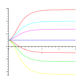
Figure 1: $\phi(r)$ vs. $\log(r)$, where numerical coefficients are $\eta=1,\beta=2,\delta=3,\mu=5$ and $g_{0}=4$. Different curves represent different asymptotic values for $K=\phi_{\infty}$. The attractor point is $\phi_{0}=1$ at the horizon, $r_{H}=1$.

Higher order results

We solve the system of equations $(EqA,EqB,Eq\Phi,EqC)$ order by order in the $x$-expansion. To first order, we find that one variables, say $\phi_{1}$, can not be fixed by the equations. Let us denote the value of $\phi_{1}$ as $K$. We thus find $a_{2}$ and $b_{1}$ as a function of $K$. One can check that at any order $n>2$, one can substitute the resulting values of $(a_{m},b_{m-1},c_{m-1})$, for all $m\leq n$ from the previous orders. Then $(EqB,Eq\Phi,EqC)$ of the current order together with $EqA$ of order $(n-1)$, consistently give,

$$b_{n}=b_{n}(K,g_{0})\;\;\;;\;\;\;a_{n+1}=a_{n+1}(K,g_{0})\;\;\;;\;\;\;\phi_{n}=\phi_{n}(K,g_{0})\;\;\;.$$ (49)

as polynomials of order $n$ in terms of $K$. It is worth noting that $K$ remains a free parameter to all orders in the $x$-expansion. From (41), (42) and (43), the asymptotic values of $(a(r),b(r),\phi(r))$ are given by a sum of all the coefficients in the x-expansion of the corresponding function. Owing to the result (49) we observe that $(a_{\infty},b_{\infty},\phi_{\infty})$ are free to take different values, given different choices for $K$ . The arbitrary value of $\phi$ at infinity is $\phi=\phi_{\infty}$, while its value at the horizon is fixed to be $\phi_{0}$. This is the very attractor mechanism which we were looking for in this model. Figure 1 shows $\phi$ vs. $r$ in logarithmic scale with different asymptotic values $K$.

5 Black Holes in Gauss-Bonnet Gravity

Since the Gauss-Bonnet case is a special sector of general $R^{2}$ gravity, it is obvious that any solution of the form considered in the previous section, enjoys the attractor mechanism. Now we relax the analyticity condition and, instead, only require the solutions to be regular at the horizon. This relaxation, enables us to cover a class of solutions connected to $G\equiv 0$ case discussed in [6], which are not analytic at $x=0$. Black holes in higher order gravity are being actively pursued. It is important to note that string theory predicts the Einstein-Hilbert action to be modified by higher order curvature corrections. The leading correction is quadratic in curvature. Typically, only certain special corrections are considered. At quadratic order, the. combination which is considered is the Gauss-Bonnet term:

$$\mathcal{R}_{\gamma\delta\lambda\sigma}R^{\gamma\delta\lambda\sigma}-4R_{\gamma\delta}R^{\gamma\delta}+R^{2}$$ (50)

We are interested in an Einstein-Gauss-Bonnet theory coupled to the gauge fields and scalars. Since the Gauss-Bonnet term in four dimensions is a topological term, the coupling to the scalar fields is crucial. Without this coupling, the Gauss-Bonnet term does not contribute to the equations of motion. In that case, we are left with the RN solution reviewed in section 2.

5.1 Equations of motion and attractors

Consider a gravity theory coupled to $U(1)$ gauge fields and scalars in the presence of higher order corrections of the Gauss-Bonnet type. The system is dictated by following bosonic action:

$$S=\frac{1}{\kappa^{2}}\int d^{4}x\sqrt{-g}\bigg{(}\;R-2(\partial\phi_{i})^{2}-f_{ab}(\phi_{i})F^{a}_{\mu\nu}F^{b\ \mu\nu}-\frac{1}{2}{\tilde{f}}_{ab}(\phi_{i})F^{a}_{\mu\nu}F^{b}_{\rho\sigma}\epsilon^{\mu\nu\rho\sigma}$$ (51)

(52)

$$+\alpha G(\phi)\mathcal{(}R_{\gamma\delta\lambda\sigma}R^{\gamma\delta\lambda\sigma}-4R_{\gamma\delta}R^{\gamma\delta}+R^{2})\bigg{)},$$ (53)

where $\alpha$ is the Gauss-Bonnet coefficient with dimensions of (length)² and is positive in Heterotic string theory. The function $G(\phi)$ is arbitrary and signifies a dilaton-like coupling. Let us also assume that all quantities are functions of $r$ and take the following ansatz for the metric and gauge fields of a Reissner-Nördstrom- Gauss-Bonnet (RNGB) black hole:

$$ds^{2} = -a(r)^{2}dt^{2}+a(r)^{-2}dr^{2}+b(r)^{2}d\Omega^{2},$$ (54)

$$F^{a} = f^{ab}(\phi_{i})(Q_{eb}-{\tilde{f}}_{bc}Q^{c}_{m})\frac{1}{b^{2}}dt\wedge dr+Q_{m}^{a}sin\theta d\theta\wedge d\phi,$$ (55)

Plugging the above ansatz in the action one finds the following one-dimensional action:

$$S=\frac{1}{\kappa^{2}}\int dr\left[2-(a^{2}b^{2})^{{}^{\prime\prime}}-2a^{2}bb^{{}^{\prime\prime}}-2a^{2}b^{2}(\partial_{r}\phi)^{2}-\frac{2V_{eff}(\phi_{i})}{b^{2}}\right.$$ (56)

(57)

$$+\left.8\,\alpha\,G(\phi)\partial_{r}\left(aa^{\prime}(-1+a^{2}b^{\prime 2})\right)\right].$$ (58)

The Hamiltonian constraint, which must be imposed in addition takes the form:

$$-1+a^{2}b^{{}^{\prime}2}+\frac{a^{2^{\prime}}b^{2^{\prime}}}{2}+\frac{1}{b^{2}}V_{eff}(\phi_{i})-a^{2}b^{2}\phi^{\prime 2}=-4\alpha G^{\prime}\left(aa^{\prime}-3a^{3}a^{\prime}b^{{}^{\prime}2}\right),$$ (59)

where a primes indicates derivation with respect to $r$. The equations of motion following from (56) are:

$$\left(a^{2}b^{2}\phi^{\prime}\right)^{\prime}=\frac{1}{2b^{2}}\frac{dV_{eff}}{d\phi} + 2\alpha\frac{dG}{d\phi}\left(aa^{\prime}\left(1-a^{2}b^{\prime 2}\right)\right)^{\prime},$$ (60)

$$\left(a^{2}b\right)^{\prime\prime}-a^{\prime 2}b-2aa^{\prime}b^{\prime}+a^{2}b\phi^{\prime 2}+\frac{V(\phi)}{b^{3}} = 4\alpha\left(\left(a^{3}a^{\prime}b^{\prime}G^{\prime}\right)^{\prime}+a^{3}a^{\prime}b^{\prime}G^{\prime\prime}\right),$$ (61)

$$bb^{\prime\prime}+b^{2}\phi^{\prime 2} = \alpha\left(-2G^{\prime\prime}+2a^{2}\left(G^{\prime}b^{\prime 2}\right)^{\prime}\right).$$ (62)

To solve the above equations, we take two different approaches: $x$-expansion and $\alpha$-expansion as explained in the following subsections.

5.2 $x$-Expansion series solutions

By $x$-expansion, we mean a set of solutions as a Frobenius series given in (41)-(43). We take a common $\lambda_{i}\equiv\lambda$ for all the solutions and write the series as:

$$\phi(r) = \phi_{0}+Kx^{\lambda}+\cdots,$$ (63)

$$a(r) = x+a_{1}x^{\lambda+1}+\cdots,$$ (65)

$$b(r) = r(1+b_{1}x^{\lambda}+\cdots).$$

Let us also consider Taylor series expansions for $V(\phi)$ and $G(\phi)$ as follows,

$$V(\phi) = v_{0}+v_{1}(\phi-\phi_{0})+\frac{1}{2}v_{2}(\phi-\phi_{0})^{2}+\cdots,$$ (67)

$$G(\phi) = g_{0}+g_{1}(\phi-\phi_{0})+\frac{1}{2}g_{2}(\phi-\phi_{0})^{2}+\cdots\>.$$ (68)

Since integer values of $\lambda$ are included in the results of section 4, we look for non-integer values $\lambda>0$, which give us a regular (though non-analytic) set of solutions at the horizon. By a careful investigation near the horizon, for the lowest power of $x$ which is $x^{\lambda}$, one can solve the set of equations together and find the non-trivial solutions as:

$$\lambda = \frac{1}{2}\left(-1+\sqrt{1+2\frac{(v_{2}+4g_{2})}{r_{H}^{2}}}\right),$$ (69)

$$v_{0}=r_{H}^{2},\;\;\;\;\;\;v_{1}=-4g_{1},$$ (70)

with $g_{1}=a_{1}=b_{1}=0$. However, $v_{2}$, $g_{2}$ and $K$ are undetermined to this order. The value of $\lambda$ in (69) is precisely what we already found in eqn. (27) with $W_{H}=V(\phi)+4G(\phi)$. The second equation in (70) is the extremum condition for $W_{H}$ which gives the attractor value $\phi_{0}$ at the horizon. Notice that we are faced with an extra condition $g_{1}=0$, which indicates that $G$, $V$ and $W_{H}$ are at their extremum at the horizon, simultaneously. Such a case would be the only situation where a non-integer $\lambda$ can be found. Otherwise we have to choose $\lambda=0$ for $g_{1}\neq 0$. The regularity condition for $\phi$ indicates that $\lambda$ should be non-negative and it in turn gives $v_{2}+4g_{2}\geq 0$. This again means that $W_{H}$ is minimum at its extremum point $\phi_{0}$. Higher order terms can be derived in a similar fashion. The important point is that, due to the non-linear nature of equations, they are a mixture of different powers of $\lambda$, like $x^{n\lambda}$ as well as $x^{n\lambda+m}$. To order these powers, we assume $0<\lambda<1$. Then the next leading term would be $x^{2\lambda}$. For higher order terms, since $\lambda$ is already known from the first order result (69), we can distinguish the next order from $x^{3\lambda}$ and $x^{\lambda+1}$. For small enough $\lambda$, it shows that we are generating a power series, $x^{n\lambda}$ as argued in [6]. Notice that in contrast to the analysis of section 3, here we considered all the equations simultaneously. This first means that, in principal, we are taking the backreaction into account. Secondly, since we are dealing with a higher derivative theory, besides the so-called Klein-Gordon equation for $\phi$ field. Other equations also involve the second derivative of $\phi$ and are important in the dynamics of $\phi$. So, they should be investigated as well.

5.3 $\alpha$-Expansion

Motivated by low energy effective actions of string theory, it is be reasonable to consider $\alpha$ as a small parameter (proportional to $\alpha^{\prime}$) and try to solve the set of equations perturbatively in the $\alpha$ parameter. Obviously, to zeroth order, we start with the results in [6]. Let us consider

$$\phi(r) = \phi^{(0)}+\alpha\phi^{(1)}(r)+\alpha^{2}\phi^{(2)}(r)+\cdots,$$ (71)

$$a(r) = \left(1-\frac{r_{H}}{r}\right)+\alpha a^{(1)}(r)+\alpha^{2}a^{(2)}(r)+\cdots,$$ (73)

$$b(r) = r\left(1+\alpha b^{(1)}(r)+\alpha^{2}b^{(2)}(r)+\cdots\right),$$

together with Taylor expansions (67) and (68). Take $\phi^{(0)}=\phi_{0}$, the constant solution at zeroth order. Then we find,

$$\phi^{(1)}=\left(1-\frac{r_{H}}{r}\right)^{(-1+\sqrt{1+2v_{2}/r_{H}})/2}+P_{4}(r),$$ (75)

where $P_{4}$ is a function of $r$ which behaves like a polynomial $x$ of order 4 near the horizon. Moreover $a^{(1)}(r)$ and $b^{(1)}(r)$ can be set to zero consistently. It is worth mentioning that the attractor equation (70) should remain valid to all orders in $\alpha$, so that when expanding in powers of $\alpha$:

$$\frac{dW_{H}}{d\phi} = \frac{d}{d\phi}\left(V(\phi)+4\alpha G(\phi)\right)|_{H}$$ (76)

$$= v_{1}+\left(v_{2}\phi^{(1)}_{H}+4g_{1}\right)\alpha+\frac{1}{2}\left(v_{2}\phi^{(2)}_{H}+v_{3}(\phi^{(1)}_{H})^{2}+8g_{2}\phi^{(1)}_{H}\right)\alpha^{2}+{\cal O}(\alpha^{3}),$$ (78)

$$= 0.$$ (80)

Solving at each order in $\alpha$, one finds:

$$v_{1} = 0,$$ (81)

$$\phi^{(1)}_{H} = -\frac{4g_{1}}{v_{2}},$$ (83)

$$\phi^{(2)}_{H} = \frac{16}{v_{2}^{3}}\left(2g_{1}g_{2}v_{2}-g_{1}^{2}v_{3}\right),$$

where the first equation is the extremum condition to zeroth order in $\alpha$ and the other two equations give the correct boundary value of the first and second order fields at the horizon, respectively.

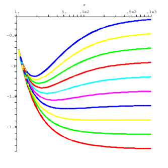
Figure 2: $\phi(r)$ vs. $\log(r)$, where numerical coefficients for the potentials are $g_{2}=v_{i\geq 2}=1$ and $g_{1}=2$. Different curves represent different asymptotic values for $\phi_{\infty}$. The attractor point is $\phi_{0}=0$ at the horizon, $r_{H}=1$.

At the second order, we one can find non-zero $a^{(2)}(r)$, $b^{(2)}(r)$ and $\phi^{(2)}(r)$, in terms of some integration constants. These constants are subject to boundary conditions which we already mentioned in section 4. Of course we have enough integration constants to satisfy all the boundary conditions. Especially, for the scalar field, we set its value at the horizon to be $\phi_{0}$ and at infinity it takes any free value. This proves the attractor behavior of the system for scalar field moduli. The $x$-expansion of $\phi^{(2)}(r)$ shows that it includes terms like $x^{n}\log{x}$ which indicate the non-analytic behavior, though regular, near the horizon. To avoid quoting lengthy results, we demonstrate our results in figure 2.

6 Conclusion

In this paper, we studied the attractor mechanism in a theory of gravity coupled to gauge fields and scalar fields, with higher derivative $R^{2}$ terms in the action. By investigating solutions of the equations of motion, we observed the attractor behavior explicitly. We looked for all possible solutions which admit the criteria of being regular at the horizon and free in the asymptotic region. The near horizon analysis done in section 3 (see also [12]), shows the criteria for attractor behavior. Although, the existence of a consistent set of solutions involving the backreaction remains far from obvious. In $R^{2}$ gravity and especially in Gauss-Bonnet theory, we solved the equations for the background and scalar fields simultaneously which means inclusion of backreaction effects. For the Gauss-Bonnet theory, given flat asymptotic boundary condition for backgrounds, the regularity of scalar fields at the horizon is a sufficient (and obviously necessary) condition to meet the attractor mechanism. The regularity at the horizon, in the non-analytic sector, sets some restriction on the effective potential $W_{H}$ which is indeed its minimality condition at its critical point. The solution with analytic behavior at the horizon appears as a new branch in the set of attractor solutions which gives no minimality restriction on the effective potential, $W_{H}$. So we observe that, compared to the case studied in [6], turning on the $R^{2}$ terms and coupling them to the moduli in the form of (44), a new sector of solutions appear for which the extremality of the effective potential is enough to produce the attractor behavior. Although, for the analysis in this paper we considered asymptotically flat space times, with the same technology, it is easy to check that attractor mechanism works as well for asymptotically (A)ds backgrounds.

Acknowledgement

Authors would like to thank B. Acharya, M. Alishahiha, A. Dabholkar, R. P. Jena, K.S. Narain, S. Randjbar-Daemi and M.M. Sheikh Jabbari for useful discussions and comments, and K. Goldstein for informing us of [5]. A.T. also thanks the Department of Theoretical Physics at TIFR for friendly hospitality. H. Y would like to thank the High Energy Group of the Abdus Salam International Centre for Theoretical Physics for hospitality and support.

References

- [1] S. Ferrara, R. Kallosh and A. Strominger, “N=2 extremal black holes,” Phys. Rev. D 52, 5412 (1995) [arXiv:hep-th/9508072].
- [2] S. Ferrara and R. Kallosh, “Supersymmetry and Attractors,” Phys. Rev. D 54, 1514 (1996) [arXiv:hep-th/9602136].
- [3] S. Ferrara and R. Kallosh, “Universality of Supersymmetric Attractors,” Phys. Rev. D 54, 1525 (1996) [arXiv:hep-th/9603090].
- [4] S. Ferrara, G. W. Gibbons and R. Kallosh, “Black holes and critical points in moduli space,” Nucl. Phys. B 500, 75 (1997) [arXiv:hep-th/9702103].
- [5] G. W. Gibbons, R. Kallosh and B. Kol, “Moduli, scalar charges, and the first law of black hole thermodynamics,” Phys. Rev. Lett. 77, 4992 (1996) [arXiv:hep-th/9607108].
- [6] K. Goldstein, N. Iizuka, R. P. Jena and S. P. Trivedi, “Non-supersymmetric attractors,” [arXiv:hep-th/0507096].
- [7] P. K. Tripathy and S. P. Trivedi, “Non-supersymmetric attractors in string theory,” [arXiv:hep-th/0511117].
- [8] K. Goldstein, R. P. Jena, G. Mandal and S. P. Trivedi, “A C-function for non-supersymmetric attractors,” [arXiv:hep-th/0512138].
- [9] R. Kallosh, “Flux vacua as supersymmetric attractors,” [arXiv:hep-th/0509112].
- [10] R. Kallosh, “New attractors,” JHEP 0512, 022 (2005) [arXiv:hep-th/0510024].
- [11] G. L. Cardoso, B. de Wit, J. Kappeli and T. Mohaupt, “Black hole partition functions and duality,” [arXiv:hep-th/0601108].
- [12] A. Sen, “Black hole entropy function and the attractor mechanism in higher derivative gravity,” JHEP 0509, 038 (2005) [arXiv:hep-th/0506177].
- [13] P. Kraus and F. Larsen, “Microscopic black hole entropy in theories with higher derivatives,” JHEP 0509, 034 (2005) [arXiv:hep-th/0506176]; P. Kraus and F. Larsen, “Holographic gravitational anomalies,” JHEP 0601, 022 (2006) [arXiv:hep-th/0508218].
- [14] M. Alishahiha and H. Ebrahim, “Non-supersymmetric attractors and entropy function,” [arXiv:hep-th/0601016].
- [15] A. Sinha and N. V. Suryanarayana, “Extremal single-charge small black holes: Entropy function analysis,” [arXiv:hep-th/0601183].
- [16] A. Sen, “Entropy function for heterotic black holes,” [arXiv:hep-th/0508042].
- [17] P. Prester, “Lovelock type gravity and small black holes in heterotic string theory,” [arXiv:hep-th/0511306].
- [18] J. M. Maldacena, A. Strominger and E. Witten, “Black hole entropy in M-theory,” JHEP 9712, 002 (1997) [arXiv:hep-th/9711053].
- [19] B. de Wit, “N = 2 electric-magnetic duality in a chiral background,” Nucl. Phys. Proc. Suppl. 49, 191 (1996) [arXiv:hep-th/9602060].
- [20] B. de Wit, “N=2 symplectic reparametrizations in a chiral background,” Fortsch. Phys. 44, 529 (1996) [arXiv:hep-th/9603191].
- [21] K. Behrndt, G. Lopes Cardoso, B. de Wit, D. Lust, T. Mohaupt and W. A. Sabra, “Higher-order black-hole solutions in N = 2 supergravity and Calabi-Yau string backgrounds,” Phys. Lett. B 429, 289 (1998) [arXiv:hep-th/9801081].
- [22] G. Lopes Cardoso, B. de Wit and T. Mohaupt, “Corrections to macroscopic supersymmetric black-hole entropy,” Phys. Lett. B 451, 309 (1999) [arXiv:hep-th/9812082].
- [23] G. Lopes Cardoso, B. de Wit and T. Mohaupt, “Deviations from the area law for supersymmetric black holes,” Fortsch. Phys. 48, 49 (2000) [arXiv:hep-th/9904005].
- [24] G. Lopes Cardoso, B. de Wit and T. Mohaupt, “Macroscopic entropy formulae and non-holomorphic corrections for supersymmetric black holes,” Nucl. Phys. B 567, 87 (2000) [arXiv:hep-th/9906094].
- [25] G. Lopes Cardoso, B. de Wit and T. Mohaupt, “Area law corrections from state counting and supergravity,” Class. Quant. Grav. 17, 1007 (2000) [arXiv:hep-th/9910179].
- [26] T. Mohaupt, “Black hole entropy, special geometry and strings,” Fortsch. Phys. 49, 3 (2001) [arXiv:hep-th/0007195].
- [27] G. Lopes Cardoso, B. de Wit, J. Kappeli and T. Mohaupt, “Stationary BPS solutions in N = 2 supergravity with R**2 interactions,” JHEP 0012, 019 (2000) [arXiv:hep-th/0009234].
- [28] G. L. Cardoso, B. de Wit, J. Kappeli and T. Mohaupt, “Examples of stationary BPS solutions in N = 2 supergravity theories with R**2-interactions,” Fortsch. Phys. 49, 557 (2001) [arXiv:hep-th/0012232].
- [29] H. Ooguri, A. Strominger and C. Vafa, “Black hole attractors and the topological string,” Phys. Rev. D 70, 106007 (2004) [arXiv:hep-th/0405146].
- [30] E. Verlinde, “Attractors and the holomorphic anomaly,” [hep-th/0412139].
- [31] H. Ooguri, C. Vafa and E. P. Verlinde, “Hartle-Hawking wave-function for flux compactifications,” Lett. Math. Phys. 74, 311 (2005) [arXiv:hep-th/0502211].
- [32] R. Dijkgraaf, R. Gopakumar, H. Ooguri and C. Vafa, “Baby universes in string theory,” [arXiv:hep-th/0504221].
- [33] A. Dabholkar, “Exact counting of black hole microstates,” Phys. Rev. Lett. 94, 241301 (2005) [arXiv:hep-th/0409148].
- [34] A. Dabholkar, R. Kallosh and A. Maloney, “A stringy cloak for a classical singularity,” JHEP 0412, 059 (2004) [arXiv:hep-th/0410076].
- [35] A. Sen, “How does a fundamental string stretch its horizon?,” JHEP 0505, 059 (2005) [arXiv:hep-th/0411255].
- [36] V. Hubeny, A. Maloney and M. Rangamani, “String-corrected black holes,” JHEP 0505, 035 (2005) [arXiv:hep-th/0411272].
- [37] D. Bak, S. Kim and S. J. Rey, “Exactly soluble BPS black holes in higher curvature N = 2 supergravity,” [arXiv:hep-th/0501014].
- [38] A. Sen, “Black holes, elementary strings and holomorphic anomaly,” JHEP 0507, 063 (2005) [arXiv:hep-th/0502126].
- [39] A. Dabholkar, F. Denef, G. W. Moore and B. Pioline, “Exact and asymptotic degeneracies of small black holes,” JHEP 0508, 021 (2005) [arXiv:hep-th/0502157].
- [40] A. Sen, “Black holes and the spectrum of half-BPS states in N = 4 supersymmetric string theory,” [arXiv:hep-th/0504005].
- [41] A. Sen, “Stretching the horizon of a higher dimensional small black hole,” JHEP 0507, 073 (2005) [arXiv:hep-th/0505122].
- [42] A. Sen, “Extremal black holes and elementary string states,” Mod. Phys. Lett. A 10, 2081 (1995) [arXiv:hep-th/9504147].
- [43] A. W. Peet, “Entropy and supersymmetry of D-dimensional extremal electric black holes versus string states,” Nucl. Phys. B 456, 732 (1995) [arXiv:hep-th/9506200].
- [44] A. Sen, “Black holes and elementary string states in N = 2 supersymmetric string theories,” JHEP 9802, 011 (1998) [arXiv:hep-th/9712150].