Gauge/String Duality in Confining Theories

Abstract:

This is the content of a set of lectures given at the “XIII Jorge André Swieca Summer School on Particles and Fields”, Campos do Jordão, Brazil in January 2005. They intend to be a basic introduction to the topic of gauge/gravity duality in confining theories. We start by reviewing some key aspects of the low energy physics of non-Abelian gauge theories. Then, we present the basics of the AdS/CFT correspondence and its extension both to gauge theories in different spacetime dimensions with sixteen supercharges and to more realistic situations with less supersymmetry. We discuss the different options of interest: placing D–branes at singularities and wrapping D–branes in calibrated cycles of special holonomy manifolds. We finally present an outline of a number of non-perturbative phenomena in non-Abelian gauge theories as seen from supergravity.

Note:

This set of lectures intends to be a basic introduction to the topic of gauge/gravity duality in confining theories. There are other sources for a nice introduction to these topics [20, 47, 79, 84]. We nevertheless attempted to keep our own perspective on the subject and hope that the final result could be seen as a valuable addition to the existing literature.

1 Lecture I: Strongly Coupled Gauge Theories

Quantum Chromodynamics (QCD) is the theory that governs the strong interaction of quarks and gluons. It is a non-Abelian quantum field theory with (color) gauge group $SU(3)$. The fundamental degrees of freedom are gluons $A_{\mu}^{k\bar{k}}$ $\in F\otimes\bar{F}$ and quarks $q_{\alpha}^{k}$ $\in F$, where $\alpha$ is a flavor index (whose values are customarily taken to be up, down, strange, charm, bottom and top) and $k,\bar{k}$ are color indices. The elementary fields are evidently charged under $SU(3)$, whose local action on the fields is

$$q_{\alpha}\to U~{}q_{\alpha}~{},~{}~{}~{}~{}~{}A_{\mu}\to UA_{\mu}~{}U^{-1}+i~{}(\partial_{\mu}U)~{}U^{-1}~{}.$$ (1)

Mesons and baryons, instead, which are made up of quarks and gluons, are singlets under the color gauge group. The $SU(3)$ invariant Lagrangian is

$${\mathcal{L}}_{QCD}=\frac{1}{4g_{YM,0}^{2}}~{}Tr\ F_{\mu\nu}F^{\mu\nu}+\frac{\theta_{YM,0}}{32\pi^{2}}~{}Tr\ F_{\mu\nu}{}^{*}F^{\mu\nu}+\sum_{\alpha=1}^{N_{f}}\bar{q}_{\alpha}(-i\gamma^{\mu}D_{\mu}+m_{\alpha})q_{\alpha}~{},$$ (2)

where $g_{YM,0}$ and $\theta_{YM,0}$ are, respectively, the bare coupling constant and $\theta$–angle, $m_{\alpha}$ the bare mass matrix of the quarks and $N_{f}$ the number of Weyl fermions. If we set $m_{\alpha}$ to zero, QCD is also invariant under

$$U(N_{f})_{L}\times U(N_{f})_{R}=SU(N_{f})_{L}\times SU(N_{f})_{R}\times U(1)_{V}\times U(1)_{A}~{},$$ (3)

at the classical level, where it also seems conformal (there are no dimensionful parameters in the Lagrangian). At the quantum level, however, instantons break the axial symmetry $U(1)_{A}$ and a quark condensate emerges $<\bar{q}_{Lk}~{}q_{R}^{~{}k}>\neq 0$ which breaks one of the $SU(N_{f})$ factors. We now review some aspects of QCD, including the striking feature that its elementary constituents, the quarks, appear to be weakly coupled at short distances and strongly coupled at long distances.

1.1 Running Coupling Constant and Asymptotic Freedom

Consider the one-loop effective action expanded around a classical QCD background. We will set in what follows $\theta_{YM}=0$. Its computation amounts to the calculus of some functional determinants, as can be immediately seen in the path integral formulation of the theory. After expansion, using the fact that a classical configuration satisfies the Euler–Lagrange equations, $S^{(1)}(\bar{A}_{\mu},\bar{q}_{\alpha})=0$, linear terms vanish (the bar over a quantity refers to its classical value). The resulting integration over the fluctuating fields is Gaussian. This implies, by means of the operatorial identity $\rm Tr\log\mathcal{O}=\log\det\mathcal{O}$, that the result can be written in terms of functional determinants

$$S^{eff}_{1-loop}=\int d^{4}x~{}\Bigg{\{}\frac{1}{4g_{YM,0}^{2}}Tr\bar{F}_{\mu\nu}\bar{F}^{\mu\nu}+\frac{1}{2}Tr\log\Delta_{1}-\frac{N_{f}}{2}Tr\log\Delta_{1/2}\Bigg{\}}~{},$$

where

$$\left(\Delta_{1}\right)^{ab}_{\mu\nu}=-\left(\bar{D}^{2}\right)^{ab}\delta_{\mu\nu}+2f^{ab}_{~{}~{}c}\bar{F}^{c}_{\mu\nu}\,,\quad\,,\quad\Delta_{1/2}=i\gamma^{\mu}\bar{D}_{\mu}~{},$$

$D_{\mu}$ is the covariant derivative and $f^{ab}_{~{}~{}c}$ are the structure constants which appear in the gauge group algebra

$$[T^{a},T^{b}]=f^{ab}_{~{}~{}c}~{}T^{c}~{}.$$

Since determinants are gauge invariant functionals of the fields a series expansion will begin with quadratic contributions in the gauge field strength, which happens to be proportional to the terms appearing in the Yang–Mills Lagrangian. This amounts to a quantum mechanical correction to the gauge coupling. Arising from a one-loop computation, we expect to get a logarithmic divergence

$$S^{eff~{}(quad)}_{1-loop}=\Bigg{(}\frac{1}{4g_{YM,0}^{2}}-\frac{b_{0}}{32\pi^{2}}\log\frac{\mu}{\Lambda}\Bigg{)}\int d^{4}x~{}Tr\bar{F}_{\mu\nu}\bar{F}^{\mu\nu}~{},$$ (4)

where $\mu$ is the energy characterizing the variation of the background field and $\Lambda$ a regulator (the scale at which we impose renormalization), while $b_{0}$ results to be the following number

$$b_{0}=-\frac{11}{3}c_{v}+\frac{4N_{f}}{3}c_{f}=-\left(11-\frac{2}{3}N_{f}\right)~{},$$ (5)

where $c_{v}=N_{c}=3$ and $c_{f}=1/2$ are Casimir values corresponding to the vector and fermion representation of the gauge group,

$$Tr_{\,r}\ (T^{a}T^{b})=c_{r}~{}\delta^{ab}~{}.$$

We immediately extract from Eq.(4) an important result: Quantum effects render $g_{YM}$ scale–dependent

$$\frac{1}{g_{YM}^{2}(\mu)}=\frac{1}{g_{YM,0}^{2}}-\frac{b_{0}}{8\pi^{2}}\log\frac{\mu}{\Lambda}~{}.$$ (6)

When there are few fermions ($N_{f}<17$), this results in a negative $\beta$–function,

$$\beta\ (g_{YM})=\frac{\partial g_{YM}}{\partial\log\frac{\mu}{\Lambda}}=-\frac{g_{YM}^{3}}{(4\pi)^{2}}\left(11-\frac{2}{3}N_{f}\right)~{}.$$ (7)

Strikingly, if we take $\mu\to\infty$, i.e. at high energies, $g_{YM}\to 0$. QCD is a perturbative theory at sufficiently high energies or short distances. The theory is analytically tractable in that regime. This is the remarkable phenomenon known as asymptotic freedom [66]. Notice that, as we reduce the energy at which the theory is probed, the coupling increases. This is shocking and in complete contrast to what happens, for example, in Quantum Electrodynamics (QED).

1.2 Dimensional Transmutation

Let us now compute the renormalization of the gauge coupling assuming $g_{YM}^{2}<<1$ for external gluons of momentum $Q$. The Renormalization Group (RG) equation can be read from the leading Feynman diagrams (Fig.1):

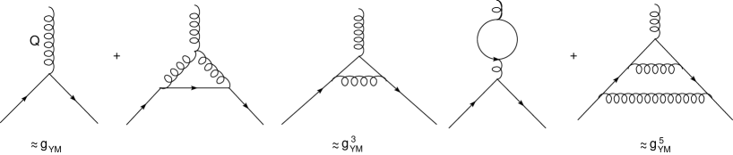
Figure 1: Leading, next-to-leading and next-to-next-to-leading perturbative contributions to the Yang–Mills coupling constant for an external gluon of momentum $Q$.

$$\frac{dg_{YM}}{dt}=\frac{b_{0}}{(4\pi)^{2}}~{}g_{YM}^{3}+\frac{2b_{1}}{(4\pi)^{4}}~{}g_{YM}^{5}+~{}\dots~{}~{}~{}~{}~{}~{}~{}t=\log\frac{Q}{\Lambda}~{},$$ (8)

where $b_{0}$ is the value computed above in (5) and $b_{1}$ is the number

$$b_{1}=-\left(51-\frac{19}{3}N_{f}\right)~{},$$

(negative for $N_{f}<9$) that will not be of great relevance to us. The Renormalization Group equation (8), including the next to leading term, can be rewritten as

$$\frac{dg_{YM}^{-2}}{dt}=-\frac{1}{8\pi^{2}}\left(b_{0}+\frac{b_{1}}{8\pi^{2}}~{}g_{YM}^{2}+~{}\dots\right)~{},$$ (9)

which, in the regime where $g_{YM}^{2}\sim-\frac{8\pi^{2}}{b_{0}}t^{-1}$ is small, can be integrated with the following result:

$$\frac{1}{g_{YM}^{2}}+\frac{b_{0}}{8\pi^{2}}\left(t-\frac{b_{1}}{b_{0}^{2}}\log t\right)+~{}\dots={\rm constant}~{}.$$ (10)

From this expression, it is straightforward to see an extremely significant consequence: we can construct a dimensionful quantity that survives the removal of the regulator:

$$Q~{}\exp\left(\frac{8\pi^{2}}{b_{0}~{}g_{YM}^{2}(Q)}\right)\left(\log\frac{Q}{\Lambda}\right)^{-\frac{b_{1}}{b_{0}^{2}}}\longrightarrow{\rm constant}~{}\Lambda~{},$$ (11)

when $t,Q\to\infty$. An energy scale appears quantum mechanically in an otherwise massless theory! This is the phenomenon known as dimensional transmutation [40]. The dynamically generated scale is customarily called  $\Lambda_{QCD}$. It is an unexpected built-in energy scale of QCD, which is experimentally found to be $\Lambda_{QCD}\approx 200MeV$.

1.3 QCD at Low Energy

As we have seen earlier, at energies high enough (higher than $\Lambda_{QCD}$), the theory is perturbative and we can use Feynman diagrams to compute particle scattering processes. When we decrease the energy,  $g_{YM}$ increases and, at some point it should be of order one or larger. The theory ceases to be well-defined perturbatively. This is in a sense welcome! Indeed, classical non-Abelian gauge theory is very different from the observed world. For QCD to successfully describe the strong force, it must have at the quantum level properties which are dramatically different from the behavior of the classical theory or perturbation theory built from it. This is telling us that the theory is strongly coupled at low energies. In particular, the following phenomena have been observed in the laboratory:

• Mass Gap:  there is a $\Delta>0$ such that every excitation of the vacuum has energy at least $\Delta$.

• Quark Confinement:  even though the theory is described in terms of elementary fields, the physical particle states (baryons, mesons, glueballs) are $SU(3)$ invariant. In a sense, the $SU(3)$ symmetry disappears in the infrared (IR).

• Chiral Symmetry Breaking:  when the quark bare masses vanish the vacuum is invariant only under a certain subgroup of the full symmetry group acting on the quark fields.  The $SU(N_{f})\times SU(N_{f})$ chiral flavor symmetry of the QCD Lagrangian is broken, as explained above, in the vacuum of the theory.  Besides, let us remind that there is also a UV breaking of a global $U(1)$ –the one that we called $U(1)_{A}$ in (3)–,

  $$q_{\alpha}~{}\to~{}e^{i\varphi\Gamma_{5}}q_{\alpha}~{},$$

  to a discrete subgroup, due to the contribution of instantons.

These are conjectured to be non-perturbative phenomena that govern the low-energy physics of QCD. There are other aspects of this nature that we will mention below. To show that this phenomenology can be actually derived from the theory of quantum chromodynamics is still an open problem. These phenomena take place in a regime of the theory which is not tractable by analytic means. How do we study strongly coupled gauge theories?.

1.4 Strings in QCD

It is natural to think that, as soon as the theory becomes strongly coupled, the relevant degrees of freedom cease to be the elementary point–like excitations of the original quantum fields. The phenomenon of color confinement might be telling us that the appropriate objects to be described are not the building blocks of classical QCD, quarks and gluons, but, for example, the confining strings formed by the collimated lines of chromoelectric flux. The underlying idea is that at low energies magnetic monopoles might become relevant, condense, and squeeze the otherwise spread chromoelectric flux into vortices (in analogy with Abrikosov vortices formed in ordinary superconductors). Thus, when studying QCD at low energies, we should change the theory to, say, a (perturbative) theory of strings describing the dynamics of these collimated flux tubes. What kind of strings are these? First of all, they are thick strings. Their thickness should be of order $1/\Lambda_{QCD}$. This seems very different from the fundamental object studied in string theory, which has zero thickness. Remarkably, it is possible to argue that thickness might be a holographic phenomenon due to the existence of extra dimensions where the strings can propagate [119].

There is another coincidence between QCD and string theory: they have a similar particle spectrum given by an infinite set of resonances, mesons and hadrons, with masses on a Regge trajectory

$$M_{J}^{2}\sim M_{0}^{2}+\frac{J}{\alpha^{\prime}}~{},$$ (12)

where $J$ is the spin and $\alpha^{\prime}$ sets the length scale (in the string picture, $1/\alpha^{\prime}$ is the string tension), that is, $\alpha^{\prime}\sim\Lambda_{QCD}^{-2}$. These were actually the reasons behind the original ideas about strings in the context of the theory of strong interactions.

Once we accept that a non–Abelian gauge theory as QCD admits a description in terms of closed strings –that is, quantum gravity– in a higher dimensional background, another important issue comes to mind. It was shown by Bekenstein [15] and Hawking [75] that the entropy of a black hole is proportional to the area of its event horizon. If gravity behaves as a local field theory we would expect, from elementary notions in statistical mechanics, the entropy of a gravitational system to be proportional to its volume. Somehow, this suggests that quantum gravity is related, to local field theories in lower dimensions in a holographic sense [82].

Gauge theory and string theory are related in a deep way which we are starting to understand. As a final piece of evidence, we shall recall that string theory has some solitonic objects called D–branes, on whose worldvolume a particular class of gauge theories live [117] which, on the other hand, are sources for the gravitational field. We will come back to this point later on. Before, let us see an interesting framework where the relation between gauge theory and string theory can be established on a solid footing.

1.5 The Large $N_{c}$ limit of Gauge Theory

A remarkable proposal was made thirty years ago by ’t Hooft [81]. Take the number of colors, $N_{c}$, from three to infinity,  $N_{c}\to\infty$ and expand in powers of $1/N_{c}$. The so–called ’t Hooft coupling,

$$\lambda\equiv g_{YM}^{2}N_{c}~{},$$ (13)

has to be held fixed in the limiting procedure. This framework provides a feasible perturbative method in terms of the ’t Hooft coupling. It is worth noticing that lattice numerical studies indicate that large $N_{c}$ is a reasonably good approximation to $N_{c}=3$ [134].

Using double line notation for gluons $A_{\mu}^{k\bar{k}}$ and quarks $q_{\alpha}^{k}$, where each line represents a gauge group index of the field, Feynman diagrams become ribbon graphs. Thus, Feynman diagrams can be drawn on closed Riemann surfaces  $\Sigma_{g}$. Vertices, propagators and loops contribute, respectively, with factors of $g_{YM}^{-2}$, $g_{YM}^{2}$ and $N_{c}$ to the diagrams. Then, a Feynman diagram including $V$ vertices, $P$ propagators and $L$ loops, contributes as $N_{c}^{\chi}$,  $\chi=V-P+L=2-2g=Eul(\Sigma_{g})$. In the large $N_{c}$ limit, a given amplitude $\mathcal{A}$ can be written as a sum over topologies

$$\mathcal{A}=\sum_{g=0}^{\infty}c_{g}(\lambda)~{}N_{c}^{2-2g}~{}.$$ (14)

When $N_{c}\to\infty$, with $\lambda$ fixed, planar Feynman diagrams dominate (see Fig.2) and we have two well distinct regimes:

• If $\lambda<<1$, also $g_{YM}<<1$,  thus, perturbative gauge theory applies and we can use Feynman diagrams.

• If $\lambda>>1$,  $\mathcal{A}$ can be rearranged in a form that reminds us of a familiar expression in string theory,

  $$\mathcal{A}=\sum_{g=0}^{\infty}g_{s}^{2g-2}\mathcal{A}_{g}(\lambda)~{},$$ (15)

  $\mathcal{A}_{g}(\lambda)$ being a perturbative closed string amplitude on $\Sigma_{g}$,  where $g_{s}\equiv 1/N_{c}<<1$ is the string coupling, and $\lambda=g_{s}N_{c}$ is a modulus of the target space.

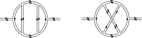
Figure 2: A plot showing two diagrams that contribute to quantum corrections of a meson mass to the same order in the coupling constant. The diagram on the left has 3 loops and will be proportional to $N_{c}^{3}$, whereas the single loop diagram on the right just contributes a factor of $N_{c}$.

Two comments are in order at this point. First, if we add quarks in the fundamental representation of the gauge group the resulting diagrams are drawn on Riemann surfaces with boundaries. This amounts to the introduction of open strings –that can be thought of as corresponding to the flux lines that bind a quark and an antiquark to form a meson– into the computation of a given amplitude. Second, it should be noticed that Feynman diagrams would span discretized Riemann surfaces that do not seem to correspond to a continuous world-sheet as that of string theory. Only very large Feynman graphs may provide a good approximation to continuous world sheets –notice that the string theory description is valid at strong coupling, where it is reasonable to assume that large Feynman graphs indeed dominate–. The idea is that a full non-perturbative description of the gauge theory will fill the holes. The results that will be discussed in these lectures point encouragingly in this direction.

In summary, strongly coupled large $N_{c}$ gauge theories are dual to (better described in terms of) perturbative closed string theories. Again, we should ask: what kind of string theories are those appearing here? Early examples of large $N_{c}$ duality, involving bosonic strings on various backgrounds that are dual to zero dimensional gauge theories (matrix models), were constructed some ten years ago [46]. In the last few years our understanding of the relation between gauge theory and string theory has been dramatically enhanced after it was realized that the former can be made to live on multi-dimensional solitonic extended objects appearing in the latter: the D–branes we mentioned earlier [117]. These gauge theories are typically supersymmetric. Thus, in order to be able to deal with these examples, let us introduce an extra ingredient: supersymmetry.

1.6 Supersymmetry and Gauge Theory

Supersymmetry relates fermions and bosons, matter and interactions. It has been proposed as a symmetry beyond the Standard Model mostly because gauge couplings unify under this principle. Indeed, if we consider a minimal supersymmetric generalization of the Standard Model where all superpartners of the known elementary particles have masses above the effective supersymmetry scale $M_{SUSY}\approx 1\,TeV$, then unification is achieved at the so-called GUT scale. Besides, supersymmetry provides a mechanism for understanding the large hierarchy in scale between the masses of the particles at the electroweak scale $M_{EW}\approx 100\,GeV$ and the GUT scale $M_{GUT}\approx 10^{16}\,GeV$. To preserve a small number such as $M_{EW}/M_{GUT}\approx 10^{-14}$ requires a fine tuning that would hardly survive quantum corrections. Due to the magic of supersymmetry, dangerous loop corrections to masses cancel to all orders in perturbation theory. In short, if unification is assumed, then it seems clear that there has to be new physics between the electroweak scale and the Planck scale and supersymmetry is a promising candidate to fill the gap.

On the other hand, from a purely theoretical point of view, supersymmetry is also extremely interesting because it allows a deeper look into the study of gauge dynamics. Supersymmetry severely constrains the theory and this leads to drastic simplifications that make it possible to deal with some of its non-perturbative aspects in many cases in an exact way. It is a symmetry that implies the appearance of robust mathematical structures on top of the gauge theory such as special geometry, holomorphicity and integrability. Furthermore, some supersymmetric systems belong to the same universality class as non-supersymmetric ones, thus opening a window to study non-perturbative phenomena of gauge theories in closely related systems.

A four–dimensional Lorentz–invariant theory can have different amounts of supersymmetry. We shall briefly recall in what follows the most interesting cases. Those aspects which are specially relevant to the content of these lectures will be discussed in greater detail later.

• $\mathcal{N}=8$  Supergravity: This is the maximal amount of supersymmetry that an interacting theory in four dimensions can possess. It is related by Kaluza–Klein reduction to the 11d Cremmer–Julia–Scherk theory [42]. It will be the subject of Dan Freedman’s lectures at this School.

• $\mathcal{N}=4$  Supersymmetric Yang–Mills Theory: It is a unique, exact and finite theory (no quantum corrections). It will be briefly discussed in the next lecture and will be considered in much greater detail by Carlos Núñez in his course. This is the gauge theory where Maldacena’s correspondence [102] applies in its full glory.

• $\mathcal{N}=2$  Supersymmetric Yang–Mills Theory: This is a theory whose low-energy dynamics has been exactly solved through the so-called Seiberg–Witten solution [128]. This solution relies heavily on special geometry and has been shown to be part of a broader framework given by the Whitham hierarchy of a given integrable system (in the absence of matter, for example, it is the periodic Toda lattice) [65, 52].

• $\mathcal{N}=1$  Supersymmetric Gauge Theory:  This theory is the closest relative of QCD: they share a number of key features that can be more easily explored in the former. Holomorphic quantities are protected by means of non-renormalization theorems [127]. This leads to a variety of exact results that we would like to keep in mind for later reference:

  1. Chiral symmetry breaking: The $U(1)$ chiral symmetry is broken by instantons to a discrete subgroup, in this case $\mathbb{Z}_{2N_{c}}$. This is a UV effect. Moreover, an IR phenomenon, gaugino condensation, further breaks the residual chiral symmetry $\mathbb{Z}_{2N_{c}}$ to $\mathbb{Z}_{2}$.

  2. Gluino condensation: there is a composite chiral field whose lowest component is $S=\rm Tr~{}\lambda\lambda$, $\lambda$ being the supersymmetric partner of the gluon, that condenses due to the existence of an IR effective superpotential $W_{eff}(S)$. This leads to $N_{c}$ isolated and degenerate vacua labeled by the value of the condensate in each, $\langle S\rangle|_{k}=e^{2\pi i\frac{k}{N_{c}}}N_{c}~{}\Lambda^{3}_{QCD}$,  $k=0,\cdots,N_{c}-1$. The coefficient $N_{c}$ is exactly calculable by instanton methods [80].

  3. $\beta$–function: The (so-called NSVZ) $\beta$–function can be computed to all orders in perturbation theory resulting in a remarkably simple expression [112]:

  $$\beta_{NSVZ}(g_{YM})=-\frac{3N_{c}g_{YM}^{3}}{16\pi^{2}}\left(1-\frac{N_{c}g_{YM}^{2}}{8\pi^{2}}\right)~{}.$$ (16)

  4. Confinement and screening of magnetic monopoles: A linear quark-antiquark potential appears in the IR. A nice mechanism that is usually advocated to implement quark confinement is the vortex formation in an Abelian Higgs model where the scalar field comes from a magnetic monopole chiral field that condenses. Indeed, the monopole-antimonopole potential can be computed and it can be checked that, instead of being confined, monopoles are screened.

  5. Confining strings: Confinement occurs when chromoelectric flux cannot spread out in space over regions larger than $\Lambda_{QCD}^{-1}$ in radius and hence forms flux tubes. The tension of these confining strings depends on the n-ality of the representation under $SU(N_{c})$ of the sources for the flux at either end of the tube. This tension has been computed in several supersymmetric approximations to QCD as well as in the lattice.

  6. Domain walls: Due to the appearance of $N_{c}$ isolated and degenerate vacua, BPS domain walls (invariant under some supersymmetry transformations) should exist interpolating between any two such vacua. Flat domain walls preserve $\frac{1}{2}$ of the supersymmetries [50]. Being BPS objects, one can compute a quantum mechanically exact formula for the tension of the wall separating the $n$-th and the $n+k$-th vacua,

  $$T_{k}=\frac{N_{c}^{2}\Lambda_{QCD}^{3}}{4\pi^{2}}~{}\sin\frac{k\pi}{N_{c}}~{}.$$ (17)

  Since $T_{k}+T_{\tilde{k}}>T_{k+\tilde{k}}$, it is clear that these domain walls tend to form a bound state. The gluing particles that carry the attractive interactions are the previously alluded glueballs.

  7. Wilson loops: Wilson loops can be used to calculate the quark anti-quark potential and determine whether a theory is confining or not. They are given by the following expression:

  $$W[\mathcal{C}]=\frac{1}{N_{c}}\rm Tr~{}P\left[e^{i\oint A}\right]~{},$$ (18)

  where $\mathcal{C}$ is some contour. If we take the contour $\mathcal{C}$ to be a rectangle (the quarks being a distance $L$ apart and the rectangle extending for a time $T$) we can read off the quark anti-quark potential $E(L)$ in the infinite strip limit, $T\to\infty$, via

  $$<W[\mathcal{C}]>=A(L)\,e^{-TE(L)}~{}.$$ (19)

  It will turn out that the calculation of the Wilson loop is simple in the context of the gauge/gravity duality, and a formula will be derived that determines whether a dual supergravity background is confining or not in terms of just two components of the metric.

  8. Instantons: As mentioned above, instantons are responsible for the symmetry breaking $U(1)_{R}\to\mathbb{Z}_{2N_{c}}$ in $\mathcal{N}=1$ supersymmetric Yang–Mills theory. They are characterized by a value of the Euclidean action

  $$S_{\rm inst}=\frac{8\pi^{2}}{g_{YM}^{2}(\mu)}+i\theta_{YM}~{}.$$ (20)

  9. Finite temperature effects: Interesting phenomena arise when the system has nonzero temperature. Thermodynamical properties of $\mathcal{N}=1$ supersymmetric Yang–Mills theory include an expected hydrodynamical behaviour near equilibrium. In this context, transport properties such as the shear viscosity, $\eta$, can be studied. Of particular interest is the ratio of $\eta$ and the entropy density $s$ of the associated plasma. In several supersymmetric gauge theories, this ratio has a universal value of $\frac{1}{4\pi}$.

  10. Adding flavors: The theory of QCD has quarks. In this sense, the addition of dynamical quarks into our analysis is clearly relevant. In particular, the introduction of flavors leads to composite states as mesons and hadrons, whose spectrum is an important observable.

  This list does not exhaust at all the plethora of non-perturbative phenomena of interest. For example, the mass spectrum of composite objects entirely built out of gluons –known as glueballs– is an interesting observable in the physics of confinement.

• $\mathcal{N}=0$  Gauge Theory:  Where we started from. Where we should eventually come back at low energies. Non-perturbative physics is hard to tackle analytically. It is, however, possible to study non-supersymmetric gauge theories by considering supersymmetric systems in higher dimensions and breaking supersymmetry upon compactification. An interesting case is given by a five dimensional theory compactified on a circle with antiperiodic boundary conditions for the fermionic fields [141].

• It is also possible to turn on a marginal deformation in the $\mathcal{N}=4$ theory that renders it less supersymmetric in the IR. In particular, this provides a window to study non-supersymmetric theories of a particular kind known as defect conformal field theories [14, 60]. There are moreover the so–called $\mathcal{N}=2^{*}$ or $\mathcal{N}=1^{*}$, which are softly broken $\mathcal{N}=4$ theories. We mention them for completeness even though we will not say anything else about these theories. Interested readers should take a look, for example, at [118].

1.7 The Large $N_{c}$ limit of Supersymmetric Gauge Theory

The large $N_{c}$ string duals of many of these theories have been discovered in the last few years. These lectures will be devoted to dig deeper in this subject but let us end this section by giving a brief outline of what is coming. The best understood case is, by far, $\mathcal{N}=4$ super Yang–Mills theory in four dimensions, whose dual is type IIB superstring theory on $AdS_{5}\times S^{5}$ [102, 67, 140]. The (conformal) gauge theory is realized on the world–volume of flat D3–branes. It is also worth mentioning that there is an interesting limit of this system whose study was extremely fruitful. From the gauge theory point of view, it consists in focusing on a sector of the theory given by states with large angular momentum, while on the string theory side it amounts to taking the Penrose limit [116, 26] which leads to type IIB superstring theory on a so called pp-wave background [16]. This conjectured duality was also extended to theories with sixteen supercharges that correspond to the low–energy dynamics of flat Dp–branes, $p\neq 3$ [85]. These are, in general, non–conformal, and the gravity/gauge theory correspondence provides a powerful tool to study the phase structure of the resulting RG flows [85]. We will discuss some aspects of these duals in the upcoming lecture.

After Maldacena’s proposal, an impressive amount of work was undertaken that allowed to understand how to extend these ideas to a variety of systems with the aim of eventually arriving some day to QCD itself. In particular, analogue results were obtained in the context of topological strings (these are given by topologically twisted sigma models [137]; we will explain more on the topological twist in lecture III). Let us state some of these results with the hope that they will become clear by the end of this set of lectures (a prudent person might prefer to avoid the following two paragraphs in a first reading of the manuscript). The so-called A-model topological string in the background of the resolved conifold, for example, is dual to 3d Chern–Simons gauge theory on $S^{3}$ [64, 114, 98]. There is also a mirrored (that is, mapped under mirror symmetry) version of this: the B–model topological string on local Calabi–Yau threefolds being dual to a holomorphic matrix model [45]. Now, topological string amplitudes are known to compute $F$–terms in related $\mathcal{N}=1$ gauge/string theories [114, 18]. This allowed Vafa [136] to conjecture that $\mathcal{N}=1$ supersymmetric Yang–Mills theory in four dimensions must be dual to either type IIA superstrings on $\mathcal{O}(-1)+\mathcal{O}(-1)\to\mathbb{P}^{1}$ with RR fluxes through the exceptional $\mathbb{P}^{1}$ or, passing through the looking glass, to type IIB superstrings on the deformed conifold with RR fluxes threading the blown–up $S^{3}$. The type IIA scenario can be uplifted to M–theory on a manifold with $G_{2}$ holonomy, where it was found that both sides of the duality are smoothly connected through a geometric transition called the flop [11]. In type IIB, instead, an interesting setup was developed by Maldacena and Núñez [106] by studying D5–branes wrapped on a supersymmetric 2–cycle in a local Calabi–Yau manifold. This opened the route to the study of a huge family of theories that can be obtained from Dp–branes wrapped on supersymmetric cycles of special holonomy manifolds. We will attempt to clarify some of these claims in the following lectures.

Finally, another kind of theories where Maldacena’s conjecture was successfully applied are constructed on D3–branes placed at the apex of Calabi–Yau cones [92, 108] as well as by considering orbifolds of type II theories. We will discuss in some detail the former case (see lecture IV), whose interest was recently revived after the discovery of an infinite family of metrics corresponding to Calabi–Yau cones on Sasaki–Einstein manifolds labeled by a set of coprime integers $Y^{p,q}$ [108], as well as $L^{a,b,c}$. These theories are superconformal in four dimensions. We will also introduce fractional branes which are responsible for destroying conformal invariance, and discuss several interesting non-perturbative physical phenomena arising in these scenarios. Most notably, the appearance of duality cascades in quiver supersymmetric gauge theories (see [132] for a recent review).

2 Lecture II: AdS/CFT Correspondence

The AdS/CFT correspondence establishes that there is a complete equivalence between $\mathcal{N}=4$ super Yang–Mills theory and type IIB string theory on $AdS_{5}\times S^{5}$ [102, 67, 140]. There is by now an impressive amount of evidence supporting this assertion (see [8] for a review). A quick attempt to motivate the subject would start by considering a stack of $N_{c}$ flat parallel D3–branes. This configuration preserves sixteen supercharges. The spectrum of massless open string states whose endpoints are located on the D3–branes is, at low energies, that of $\mathcal{N}=4$ $U(N_{c})$ super Yang–Mills theory in four dimensions, whose main features will be shortly addressed later on this lecture. On the other hand, from the closed string theory point of view, these D3–branes source some fields that satisfy the field equations of type IIB supergravity . The solution reads, in the string frame,

$$ds^{2}=H_{3}^{-\frac{1}{2}}dx_{1,3}^{2}+H_{3}^{\frac{1}{2}}(dr^{2}+r^{2}d\Omega_{5}^{2})~{},$$ (21)

$$e^{2\phi}=e^{2\phi_{\infty}}=const~{},$$ (22)

$$F_{[5]}=(1+\star)~{}dH_{3}^{-1}\wedge dx^{0}\wedge dx^{1}\wedge dx^{2}\wedge dx^{3}~{},$$ (23)

where $d\Omega_{5}^{2}$ is the round metric on $S^{5}$, $\star$ stands for the Hodge dual, and $H_{3}$ is a harmonic function of the transverse coordinates

$$H_{3}=1+4\pi g_{s}N_{c}\frac{{\alpha^{\prime}}^{2}}{r^{4}}~{}.$$ (24)

The idea now is to realize that it is possible to decouple the open and closed string massive modes by taking the limit $\alpha^{\prime}\to 0$. As the Planck length is given by $l^{2}_{P}=g_{s}^{1/2}\alpha^{\prime}$ and $g_{s}$ is constant, we see that this limit also decouples the open/closed interactions, $l_{P}\to 0$. An important point is that the Yang–Mills coupling, $g^{2}_{YM}$, remains finite,

$$g^{2}_{YM}=4\pi g_{s}~{},$$ (25)

in the low energy effective action. The limit $\alpha^{\prime}\to 0$ leads, in the string theory side, to type IIB supergravity. The right limiting procedure also involves a near-horizon limit, $r\to 0$, such that

$$U\equiv\frac{r}{\alpha^{\prime}}=\mbox{fixed}~{},~{}~{}~{}~{}~{}r,\alpha^{\prime}\to 0~{},$$ (26)

where we would like the reader to notice that $U$ has dimensions of energy. Performing such a limit in the supergravity solution (21), we obtain

$$ds^{2}={\alpha^{\prime}}\;\Bigg{[}\frac{{\alpha^{\prime}}\,U^{2}}{L^{2}}~{}dx_{1,3}^{2}+\frac{L^{2}}{{\alpha^{\prime}}\,U^{2}}~{}\Bigg{(}dU^{2}+U^{2}\,d\Omega_{5}^{2}\Bigg{)}\Bigg{]}~{},$$ (27)

where we have introduced the characteristic scale parameter $L$,

$$L^{4}=4\pi g_{s}N_{c}{\alpha^{\prime}}^{2}~{}.$$ (28)

It is not difficult to check that the metric above corresponds to the direct product of $AdS_{5}\times S^{5}$ with both spaces having the same radius, $L$, and opposite constant curvature, $\mathcal{R}\sim\pm\,L^{-2}$. The dilaton is also constant. If we take the limit $g_{s}\to 0$, $N_{c}\to\infty$ with $g_{s}N_{c}$ constant and large enough, we see that $L$ is also large and the type IIB supergravity description is perfectly valid for any value of $U$. Let us finally notice that the curvature and the ’t Hooft coupling are inversely proportional, $\alpha^{\prime}\mathcal{R}\sim\lambda^{-1/2}$. This means that the gauge theory description and the string/gravity one are complementary and do not overlap. The AdS/CFT correspondence is an example of a strong/weak coupling duality. That is, the system is well described by $\mathcal{N}=4$ $U(N_{c})$ super Yang–Mills theory for small values of the ’t Hooft coupling while it is better described by type IIB string/gravity theory whenever $\lambda$ gets large. In spite of the fact that this issue makes it extremely hard to prove or disprove the AdS/CFT correspondence, there are several quantities that are known to be independent of the coupling and whose computation using both descriptions coincides.

There are arguments that will not be discussed in these lectures pointing towards the fact that the Maldacena conjecture might be stronger than what we have presented here. We might state three different versions of the conjecture which, in increasing level of conservatism, can be named as the strong, the mild and the weak. They are described in Table 1, where the appropriate limits that are assumed on the parameters of the theory are also mentioned.

Gravity side Gauge Theory side Type IIB string theory $\mathcal{N}=4$ $SU(N_{c})$ super on $AdS_{5}\times S^{5}$ Yang–Mills theory Strong $\forall g_{s},~{}L^{2}/\alpha^{\prime}$ $\forall g_{YM},~{}N_{c}$ Classical type IIB strings ’t Hooft large $N_{c}$ limit of on $AdS_{5}\times S^{5}$ $\mathcal{N}=4$ $SU(N_{c})$ SYM Mild $g_{s}\to 0,~{}L^{2}/\alpha^{\prime}$ fixed $N_{c}\to\infty\,,~{}\lambda=g_{YM}^{2}N_{c}$ fixed Classical type IIB supergravity Large ’t Hooft coupling limit on $AdS_{5}\times S^{5}$ of $\mathcal{N}=4$ $SU(N_{c})$ SYM Weak $g_{s}\to 0,~{}L^{2}/\alpha^{\prime}\to\infty\,$ $N_{c}\to\infty\,,~{}\lambda\to\infty\,$

Table 1: Three versions of the Maldacena conjecture: the strong, the mild and the weak.

Let us briefly discuss some basic aspects of the conjecture that will be important in the rest of the lectures. We start by presenting the basics of $\mathcal{N}=4$ supersymmetric Yang–Mills theory.

2.1 $\mathcal{N}=4$ Supersymmetric Yang–Mills Theory

Four dimensional $\mathcal{N}=4$ supersymmetric theory is special in that it has a unique superfield in a given representation of the gauge group. Let us take it to be the adjoint representation. The field content of the supermultiplet consists of a vector field $A_{\mu}$, six scalars $\phi^{I}$ $I=1,...,6$, and four fermions $\chi_{\alpha}^{i}$, $\chi_{\dot{\alpha}}^{\bar{i}}$, where $\alpha$ and $\dot{\alpha}$ are chiral indices while $i=1,2,3,4$ and $\bar{i}$ are in the ${\bf 4}$ and ${\bf\bar{4}}$ of the $R$-symmetry group $SU(4)=SO(6)$. It is a global internal symmetry of $\mathcal{N}=4$ supersymmetric Yang–Mills theory. The supercharges also belong to these representations of $SO(6)$. Notice that it acts as a chiral symmetry. The Lagrangian contains two parameters, the coupling constant $g_{YM}$ and the theta angle $\theta_{YM}$,

$$\mathcal{L}_{\mathcal{N}=4} = Tr\left[\frac{1}{g_{YM}^{2}}\bigg{(}F\wedge\star F+(D\phi)^{2}+\sum_{IJ}[\phi^{I},\phi^{J}]^{2}\bigg{)}+\theta_{YM}~{}F\wedge F\right]$$ (30)

$$~{}~{}~{}~{}~{}+\frac{1}{g_{YM}^{2}}Tr\left[\bar{\chi}\not\!\!D\chi+\bar{\chi}\Gamma^{I}\phi^{I}\chi\right]~{}.$$

The theory is scale invariant quantum mechanically. Indeed, just by counting the degrees of freedom of the supermultiplet, it is immediate to see that the $\beta$–function is zero to all orders. Thus, it is conformal invariant. This gives raise to sixteen conformal supercharges (in any conformal theory, the supersymmetries are doubled). The theory is maximally supersymmetric. It displays a (strong/weak) S–duality under which the complexified coupling constant

$$\tau_{YM}=\frac{\theta_{YM}}{2\pi}+\frac{4\pi i}{g^{2}_{YM}}~{},$$ (31)

transforms into $-1/\tau_{YM}$. This combines with shifts in $\theta_{YM}$ to complete the group $SL(2,\mathbb{Z})$. As we saw in (25), there is a relation between the Yang–Mills coupling, on the gauge theory side, and the string coupling. This relation has to be supplemented by another one that links the $\theta$–angle with the vacuum expectation value of the RR scalar $\chi$,

$$\theta_{YM}=2\pi\chi~{},$$ (32)

such that the $SL(2,\mathbb{Z})$ symmetry is clearly connected with the usual S–duality symmetry in type IIB string theory.

2.2 Symmetries and Isometries

The $AdS_{5}$ factor can be thought of, after a simple change of variables to adimensional coordinates $U=\frac{L}{\alpha^{\prime}}\,e^{r}$ and $dx_{1,3}^{2}\to L^{2}\,dx_{1,3}^{2}$, as a warped codimension one 4d Minkowski space –this actually guarantees the Poincaré invariance of the gauge theory, as reflected in the appearance of a Minkowskian 4d factor–, whose line element reads

$$ds^{2}=L^{2}(dr^{2}+e^{2r}dx_{1,3}^{2})~{}.$$ (33)

The limit where the radial coordinate goes to infinity, $r\to\infty$, and the exponential factor blows up is called the boundary of $AdS_{5}$. String theory excitations extend all the way to the boundary where the dual gauge theory is interpreted to live [28]. When this space is written as a hypersurface embedded in $\mathbb{R}^{2,4}$,

$$-w_{1}^{2}-w_{2}^{2}+x_{1}^{2}+x_{2}^{2}+x_{3}^{2}+x_{4}^{2}=-L^{2}~{};$$ (34)

it is manifest that it possesses an $SO(2,4)$ isometry group. The remaining $S^{5}$ factor of the background provides an extra $SO(6)$ isometry. Now, it is not a coincidence that $SO(2,4)$ is the conformal group in 4d, while $SO(6)\approx SU(4)$ is exactly the $R$–symmetry group of $\mathcal{N}=4$ supersymmetric Yang–Mills theory. The bosonic global symmetries match perfectly. There are also fermionic symmetries which, together with the bosonic ones, form the supergroup $PSU(2,2|4)$. It is possible to verify that both the massless fields in string theory and the BPS operators of supersymmetric Yang–Mills theory, whose precise matching is not discussed here, are classified in multiplets of this supergroup [140].

2.3 Correlators

Consider a free massive scalar field propagating in $AdS_{5}$. Its equation of motion is the Klein–Gordon equation,

$$(\Box+m^{2})~{}\phi=0~{},$$ (35)

which has two linearly independent solutions that behave asymptotically as exponentials

$$\phi\approx e^{(\Delta-4)r}~{},~{}~{}~{}{\rm and}~{}~{}~{}~{}~{}\phi\approx e^{-\Delta r}~{},$$ (36)

with $\Delta=2+\sqrt{4+m^{2}L^{2}}$. The first solution dominates near the boundary of the space while the second one is suppressed. Now consider a solution of the supergravity equations of motion whose asymptotic behavior is

$$\Phi_{i}(r,x^{\mu})\sim\varphi_{i}(x^{\mu})~{}e^{(\Delta_{i}-4)r}~{},$$ (37)

where the $x^{\mu}$ are gauge theory coordinates living at the boundary. An operator $\mathcal{O}_{i}$ in the gauge theory is associated with fluctuations of its dual supergravity field (this identification is non-trivial). More precisely, the generating functional for correlators in the field theory is related to the type IIB string theory partition function by [67, 140]

$$\mathcal{Z}_{\rm string}\left[\Phi_{i}\right]=\bigg{<}\exp\bigg{(}\int d^{4}x~{}\varphi_{i}\mathcal{O}_{i}\bigg{)}\bigg{>}~{},$$ (38)

subject to the relevant boundary conditions (37). This is a deep and extremely relevant entry in the AdS/CFT dictionary. For most applications, we really have to deal with the saddle-point approximation of this formula,

$$\exp\left(-\Gamma_{\rm sugra}[\Phi_{i}]\right)\approx\bigg{<}\exp\bigg{(}\int d^{4}x~{}\varphi_{i}\mathcal{O}_{i}\bigg{)}\bigg{>}~{},$$ (39)

where $\Gamma_{\rm sugra}[\Phi_{i}]$ is the supergravity action evaluated on the classical solution. It turns out that the operator $\mathcal{O}_{i}$ has conformal dimension $\Delta_{i}$. This is a nontrivial prediction of AdS/CFT. The brief discussion here has only involved scalar fields. It naturally extends to all degrees of freedom in $AdS_{5}$: this dictionary implies that for every gauge invariant operator in the gauge theory there exists a corresponding closed string field on $AdS_{5}\times S^{5}$ whose mass is related to the scaling dimension of the operator and vice-versa. We will comment in the last lecture on some additional features of the AdS/CFT correspondence that arise when studying the gravity duals of confining gauge theories.

2.4 Theories with Sixteen Supercharges

Consider now a stack of $N_{c}$ flat Dp–branes. This configuration preserves sixteen supercharges. The light open string spectrum is that of a $U(N_{c})$ super Yang–Mills theory in p+1 dimensions. We would thus expect maximally supersymmetric Yang–Mills theory in p+1 dimensions to be dual to type IIA/IIB string theory in the near horizon limit of the p-brane supergravity solution. This solution reads (in the string frame):

$$ds^{2}=H_{p}^{-\frac{1}{2}}dx_{1,p}^{2}+H_{p}^{\frac{1}{2}}(dr^{2}+r^{2}d\Omega_{8-p}^{2})~{},$$ (40)

$$e^{-2(\phi-\phi_{\infty})}=H_{p}^{\frac{p-3}{2}}~{},$$ (41)

$$A_{[p+1]}=-\frac{1}{2}(H_{p}^{-1}-1)~{}dx^{0}\wedge\dots\wedge dx^{p}~{},$$ (42)

where $d\Omega_{8-p}^{2}$ is the round metric on $S^{8-p}$ and $H_{p}$ is a harmonic function of the transverse coordinates

$$H_{p}=1+2^{5-p}\pi^{\frac{5-p}{2}}g_{s}N_{c}\,\Gamma\left(\frac{7-p}{2}\right)\frac{{\alpha^{\prime}}^{\frac{7-p}{2}}}{r^{7-p}}~{}.$$ (43)

There are however new problems as soon as we abandon  $p=3$. In order to generalize the Maldacena correspondence, we should keep in mind that it is necessary to decouple both the open and closed string massive modes (that is, $\alpha^{\prime}\rightarrow 0$) as well as the open/closed interactions (correspondingly, the Planck length $l^{2}_{P}=g_{s}^{1/2}\,\alpha^{\prime}\rightarrow 0$), while maintaining a finite $g^{2}_{YM}$,

$$g^{2}_{YM}=(2\pi)^{p-2}g_{s}\,(\alpha^{\prime})^{\frac{p-3}{2}}~{},$$ (44)

in the low energy effective action. (We will derive this relation by the end of the present lecture.) The latter condition implies that $g_{s}\sim(\alpha^{\prime})^{\frac{3-p}{2}}$ in the field theory limit which, combined with the other requirements, forces the string coupling to diverge for $p>3$. Moreover, plugging this expression into the condition on the Planck length, we get  $l_{P}\sim(\alpha^{\prime})^{\frac{7-p}{8}}\rightarrow 0$  as  $\alpha^{\prime}\to 0$. Thus, we should restrict our attention to $p<7$. Naively, we would conclude that the decoupling is not possible for Dp–branes with $p\geq 7$  and the dual strong coupling description is needed for D4, D5 and D6–branes. However, the situation is more subtle than this due to the fact that the string coupling depends on the radial variable. Indeed, the near-horizon limit,

$$U\equiv\frac{r}{\alpha^{\prime}}=\mbox{fixed}~{},~{}~{}~{}~{}~{}r,\alpha^{\prime}\to 0~{},$$ (45)

of the supergravity solution (40)–(42) corresponding to $N_{c}$ Dp–branes reads

$$ds^{2}=\alpha^{\prime}\bigg{[}\bigg{(}\frac{d_{p}\,g^{2}_{YM}N_{c}}{U^{7-p}}\bigg{)}^{-\frac{1}{2}}dx_{1,p}^{2}+\bigg{(}\frac{d_{p}\,g^{2}_{YM}N_{c}}{U^{7-p}}\bigg{)}^{\frac{1}{2}}\left(dU^{2}+U^{2}d\Omega_{8-p}^{2}\right)\bigg{]}~{},$$ (46)

$$e^{\phi}=(2\pi)^{2-p}g_{YM}^{2}\left(\frac{d_{p}\,g^{2}_{YM}N_{c}}{U^{7-p}}\right)^{\frac{3-p}{4}}~{},$$ (47)

where

$$d_{p}=2^{7-2p}\pi^{\frac{9-3p}{2}}\Gamma\left(\frac{7-p}{2}\right)~{}.$$

From the field theory point of view, $U$ is an energy scale. The near horizon limit of Dp–brane solutions has non-constant curvature for $p\neq 3$,

$$\alpha^{\prime}~{}\mathcal{R}\sim\frac{1}{g_{eff}}\sim\bigg{(}\frac{U^{3-p}}{d_{p}\,g^{2}_{YM}N_{c}}\bigg{)}^{\frac{1}{2}}~{}.$$ (48)

We have introduced in this equation a dimensionless coupling, $g^{2}_{eff}\sim g_{YM}^{2}N_{c}U^{p-3}$, which is particularly useful as long as the Yang–Mills coupling is dimensionful for gauge theories in dimensions other than four. It is proportional to the inverse of the curvature, which means that the gauge theory description and the string/gravity one are complementary and do not apply at the same energy scale. Notice that the dilaton is not constant either, so the ranges of validity of the various descriptions become more complicated here. The decoupling limit does not work so cleanly. The supergravity solution is valid in regions where  $\alpha^{\prime}\mathcal{R}\ll 1$ and $e^{\phi}\ll 1$. These conditions result to be energy dependent. In particular, we see that for $p<3$ the effective coupling is small at large $U$ and the theory becomes UV free. Instead, for $p>3$ the situation is the opposite, the effecting coupling increases at high energies and we have to move to the dual string/gravity description. This reflects the fact that for $p>3$ supersymmetric Yang–Mills theories are non-renormalizable and hence, at short distances, new degrees of freedom appear [85].

The isometry group of the resulting metric is $ISO(1,p)\times SO(9-p)$ for $p\neq 3$. There is no $AdS$ factor, something that reflects the fact that the dual supersymmetric theories are not conformally invariant. Again, there is a matching of symmetries at work. The $ISO(1,p)$ factor clearly corresponds to the Poincaré symmetry of the supersymmetric Yang–Mills theory, while $SO(9-p)$ is the $R$–symmetry. It is an $R$–symmetry since spinors and scalars on the worldvolume of the Dp–brane transform respectively as spinors and a vector in the directions transverse to the brane; hence, under $SO(9-p)$. Let us consider a couple of examples that will be useful in the following lectures.

2.4.1 The case of Flat D5–branes

In this subsection we use the formulas presented above to analyze the decoupling limit, $r,\alpha^{\prime}\to 0$, for $N_{c}$ D5–branes. The Yang–Mills coupling has to be held fixed in this limit, $g^{2}_{YM}=(2\pi)^{3}g_{s}\,\alpha^{\prime}$ and the resulting solution is

$$ds^{2}=\alpha^{\prime}\bigg{[}\bigg{(}\frac{8\pi^{3}\,U^{2}}{g^{2}_{YM}N_{c}}\bigg{)}^{\frac{1}{2}}dx_{1,5}^{2}+\bigg{(}\frac{g^{2}_{YM}N_{c}}{8\pi^{3}\,U^{2}}\bigg{)}^{\frac{1}{2}}\left(dU^{2}+U^{2}d\Omega_{3}^{2}\right)\bigg{]}~{},$$ (49)

$$e^{\phi}=\frac{g_{YM}U}{(2\pi)^{3/2}\sqrt{N_{c}}}~{}.$$ (50)

We can see that there are different energy scales where the system is described in different ways. Perturbative super Yang–Mills is valid in the deep IR region,

$$g^{2}_{eff}=g^{2}_{YM}N_{c}U^{2}\ll 1~{}~{}~{}\Rightarrow~{}~{}~{}g_{YM}U\ll\frac{1}{\sqrt{N_{c}}}~{}.$$ (51)

Let us now consider what happens as we increase the energy. The conditions for supergravity to be a valid approximation, namely that the curvature in string units and the string coupling remain small are:

$$\alpha^{\prime}~{}\mathcal{R}\ll 1~{}~{}~{}~{}~{}{\rm and}~{}~{}~{}~{}~{}e^{\phi}\ll 1~{},$$ (52)

and we see that this happens within an energy window

$$\frac{1}{\sqrt{N_{c}}}\ll g_{YM}U\ll\sqrt{N_{c}}~{}.$$ (53)

In this range of energies we can trust the type IIB D5–brane supergravity solution and it provides an appropriate description of the system. At higher energies, $g_{YM}U\gg\sqrt{N_{c}}$, the string coupling becomes large and we need to perform an S–duality transformation to describe the system in terms of the supergravity solution corresponding to flat NS5–branes. In particular, $\tilde{\alpha}^{\prime}=g_{s}\alpha^{\prime}=g^{2}_{YM}/(2\pi)^{3}$, and after S–duality is applied, the solution reads,

$$ds^{2}=dx_{1,5}^{2}+\tilde{\alpha}^{\prime}\bigg{(}\frac{N_{c}}{U^{2}}\,dU^{2}+N_{c}\,d\Omega_{3}^{2}\bigg{)}~{},$$ (54)

and the string coupling gets inverted. The curvature in string units of this solution, $\tilde{\alpha}^{\prime}\mathcal{R}\sim N_{c}^{-1}$, is still small for large $N_{c}$ and the supergravity solution is therefore valid.

2.4.2 The case of Flat D6–branes

After taking the decoupling limit for $N_{c}$ D6–branes, while keeping as usual the Yang–Mills coupling fixed, $g^{2}_{YM}=(2\pi)^{4}g_{s}\,(\alpha^{\prime})^{3/2}$,

$$ds^{2}=\alpha^{\prime}\bigg{[}\frac{(2\pi)^{2}}{g_{YM}}\bigg{(}\frac{2U}{N_{c}}\bigg{)}^{\frac{1}{2}}dx_{1,6}^{2}+\frac{g_{YM}}{(2\pi)^{2}}\bigg{(}\frac{N_{c}}{2U}\bigg{)}^{\frac{1}{2}}\left(dU^{2}+U^{2}d\Omega_{2}^{2}\right)\bigg{]}~{},$$ (55)

$$e^{\phi}=\frac{g_{YM}^{2}}{2\pi}\left(\frac{2U}{g^{2}_{YM}N_{c}}\right)^{\frac{3}{4}}~{},$$ (56)

we see that the perturbative super Yang–Mills description is valid in the deep IR region,

$$g^{2}_{eff}=g^{2}_{YM}N_{c}U^{3}\ll 1~{}~{}~{}\Rightarrow~{}~{}~{}U\ll\frac{1}{(g_{YM}^{2}N_{c})^{\frac{1}{3}}}~{}.$$ (57)

For higher energies, the type IIA supergravity solution is valid to describe the system at energy scales in the interval

$$\frac{1}{(g_{YM}^{2}N_{c})^{\frac{1}{3}}}\ll U\ll\frac{N_{c}}{g_{YM}^{2/3}}~{}.$$ (58)

In the UV, that is for energies above $U\gg N_{c}/g_{YM}^{2/3}$, the dilaton grows and the 11th dimensional circle opens up with radius $R_{11}(U)\gg l_{p}$: we have to uplift the IIA solution to M–theory. This uplift results in a purely gravitational background, the Ramond-Ramond potential $(C_{[1]})_{\mu}$ to which the D6–brane couples magnetically lifts to the metric components $g^{(11)}_{\natural\mu}$, where $\natural$ denotes the 11th dimension. The actual solution in 11d reads, after a change of variable of the form $y^{2}=2N_{c}g_{YM}^{2}U/(2\pi)^{4}$,

$$ds^{2}_{11d}=dx_{1,6}^{2}+dy^{2}+y^{2}\left(d\theta^{2}+\sin^{2}\theta d\varphi^{2}+\cos^{2}\theta d\phi^{2}\right)~{},$$ (59)

where the angular variables are identified upon shifts

$$(\varphi,\phi)\sim\left(\varphi+\frac{2\pi}{N_{c}},\phi+\frac{2\pi}{N_{c}}\right)~{},~{}~{}~{}~{}~{}0\leq\theta<\frac{\pi}{2}~{},~{}~{}~{}0\leq\varphi,\phi<2\pi~{},$$ (60)

thus describing an asymptotically locally Euclidean (ALE) space with an $SU(N_{c})$ singularity. This amounts to the fact that the $S^{3}$ metric in (59–60) is written as a $U(1)$ bundle over $S^{2}$ with monopole charge $N_{c}$. An interesting point to keep in mind is that D6–branes provide a purely gravitational background as seen from eleven dimensional M–theory. The metric is locally flat, so that the curvature vanishes everywhere except at the singularities. At very large values of $y$ (that is, in the far UV), the proper length of circles is of order $R_{circles}\sim g_{YM}N_{c}^{-1/2}U^{1/2}$ while $l_{P}^{(11)}=g_{s}^{1/3}l_{s}$: an everywhere flat 11d background as long as $R_{circles}\gg l_{P}^{(11)}~{}\Rightarrow~{}U\gg\frac{N_{c}}{g_{YM}^{2/3}}$. As a result of this, it is not necessary to be in the large $N_{c}$ limit to trust that 11d supergravity provides a good description in the UV. However, when a massive radial geodesic in the IIA near-horizon D6–brane background runs away from the small $U$ region, it starts seeing the extra 11th dimension and the geometry becomes flat, so that it can easily escape to infinity. Decoupling is spoiled. The proper description should then be the whole M-theory (and not just supergravity excitations) in the ALE space background.

2.5 The D–brane world-volume action

Let us end this lecture by rapidly mentioning some aspects of the world-volume low-energy description of Dp–branes. We have already mentioned that the massless string states on a Dp–brane form the vector multiplet of a $(p+1)$–dimensional gauge theory with sixteen supercharges. Consider a single Dp–brane with world-volume $\mathcal{M}_{p+1}$, whose coordinates are $\xi^{a}$. The bosonic part of its world-volume action is given by the sum of the Dirac–Born–Infeld part and the Wess–Zumino part

$$S_{Dp} = -\tau_{p}\int_{\mathcal{M}_{p+1}}d^{p+1}\xi\ e^{-\Phi}\sqrt{-\det\left(\hat{G}_{ab}+\hat{B}_{ab}+2\pi\alpha^{\prime}F_{ab}\right)}$$ (62)

$$~{}~{}~{}~{}~{}+\tau_{p}\int_{\mathcal{M}_{p+1}}\sum_{q}\hat{C}_{[q]}\wedge e^{\hat{B}_{[2]}+2\pi\alpha^{\prime}F}~{},$$

where hats denote pull-backs of bulk fields onto the world-volume of the Dp–brane, $C_{[q]}$ are the RR potentials, and $F$ is the world-volume gauge field strength. The tension of the Dp–brane is $\tau_{p}$, and the fact that the RR couplings are equal to the tension is telling us that these are BPS objects. Let us study the low-energy dynamics of this action. Consider the static gauge $x^{a}=\xi^{a}$ and $x^{I}=x^{I}(\xi^{a})$, which can always be fixed because of diffeomorphism invariance. The DBI action can be expanded at low energies in powers of $\alpha^{\prime}$,

$$\sqrt{-\det\left(\hat{G}_{ab}+\hat{B}_{ab}+2\pi\alpha^{\prime}F_{ab}\right)}=\sqrt{-\det G_{ab}}~{}\times$$ (63)

$$~{}~{}~{}~{}~{}~{}~{}\times\left\{1+\frac{1}{2}G^{ab}G_{IJ}\partial_{a}x^{I}\partial_{b}x^{J}+\frac{(2\pi\alpha^{\prime})^{2}}{4}G^{ac}G^{bd}F_{ab}F_{cd}\right\}~{}.$$ (64)

Now, plugging this expansion in to (62), and using the explicit solution (40)–(42), the action becomes

$$S_{Dp} \simeq -\tau_{p}\int d^{p+1}x\ \left\{H_{p}^{-1}+\frac{1}{2}\partial_{a}x^{I}\partial_{a}x^{I}+\frac{(2\pi l_{s}^{2})^{2}}{4}F_{ab}F_{ab}\right\}$$ (66)

$$~{}~{}~{}~{}~{}+\tau_{p}\int d^{p+1}\xi\ (H_{p}^{-1}-1)~{}.$$

If we neglect a constant term, and define $x^{I}=2\pi\alpha^{\prime}\Phi^{I}$, the action simplifies to

$$S_{Dp}=-\tau_{p}\frac{(2\pi\alpha^{\prime})^{2}}{2}\int d^{p+1}x\ \bigg{\{}\frac{1}{2}\partial_{a}\Phi^{I}\partial_{a}\Phi^{I}+\frac{1}{4}F_{ab}F_{ab}\bigg{\}}~{},$$ (67)

which is precisely the kinetic (bosonic) part of the $(p+1)$–dimensional supersymmetric gauge theory action, after the identification

$$g_{YM}^{2}=\frac{2}{(2\pi\alpha^{\prime})^{2}\tau_{p}}=(2\pi)^{p-2}g_{s}\,(\alpha^{\prime})^{\frac{p-3}{2}}~{},$$ (68)

where we have replaced the value of the tension of a Dp–brane, and this is the origin of eq.(44) which we used above.

If we put $N_{c}$ Dp–branes on top of each other, there are some difficulties and ambiguities in writing the corresponding world-volume action. However, all attempts that have been considered in the literature have resulted in the same low-energy dynamics: the natural extension of the formulas above to the non–Abelian case.

3 Lecture III: Reducing Supersymmetry and Breaking Conformal Invariance

The scaling arguments behind decoupling gravity from gauge theories living in D–branes do not rely on maximal supersymmetry. As such, one might be reasonably interested in generalizing the AdS/CFT correspondence to supersymmetric gauge theories with less than sixteen supercharges. In order to make contact with Nature, we need to reduce the number of supersymmetries and to spoil conformal invariance.

We might proceed by deforming $\mathcal{N}=4$ supersymmetric Yang–Mills theory by adding a relevant or marginal operator which breaks conformal invariance and supersymmetry, for example a mass term $M$ or a superpotential term, into the action and exploring the corresponding deformation in the gravity dual. In this way, the theories would be conformal in the UV (asymptotically $AdS$ configurations). In general, these scenarios lead to a RG invariant scale given by

$$\Lambda_{QCD}\sim Me^{-\frac{1}{g_{YM}^{2}N_{c}}}~{},$$ (69)

which means that the decoupling can only be attained if we let $M\to\infty$ together with $\lambda=g_{YM}^{2}N_{c}\to 0$, so that $\Lambda_{QCD}$ is kept fixed. As $\lambda\to 0$, there is little hope to apply this deformation method to study strongly coupled QCD via supergravity. The masses $M$ of the unwanted degrees of freedom do not decouple from the theory before the strong-coupling phase is reached. We will not further discuss this line of thought and the interested reader should take a look at references [7, 118].

We will instead follow a different approach. We will engineer D–brane configurations of type II string theory (or M–Theory) which accomplish one or both of the following features:

• reduce supersymmetry by considering an appropriate closed string background known to preserve a specific fraction of the supersymmetries of flat space or

• break conformal symmetry by engineering particular configurations of D–branes in the above closed string backgrounds.

Roughly speaking, what we need is to modify the flatness of the D–branes, the flatness of the target spaces, or both simultaneously.

3.1 Closed String Backgrounds with Reduced Supersymmetry

Consider a bosonic background. We say that it is supersymmetric or that it preserves supersymmetry if it is invariant under supersymmetry transformations with spinor parameter $\epsilon$. The number of linearly independent solutions for $\epsilon$ determines the amount of supersymmetry it preserves. We are therefore looking for a supersymmetric parameter $\epsilon$ that fullfils

$$\delta_{\epsilon}~{}\Phi_{b}|_{sol}\sim\Psi_{f}|_{sol}=0~{},$$ (70)

$$\delta_{\epsilon}~{}\Psi_{f}|_{sol}\sim\Phi_{b}|_{sol}=0~{},$$ (71)

for bosonic ($\Phi_{b}$) and fermionic ($\Psi_{f}$) fields. For a bosonic solution the latter one is the non-trivial requirement. Indeed, it amounts to first order differential equations that the bosonic fields must obey, the so-called BPS equations. Among them, the transformation law of the gravitino, in the absence of RR fields, reads $\delta_{\epsilon}\Psi_{\mu}=D_{\mu}\epsilon$. Therefore, supersymmetric backgrounds are given by Ricci-flat manifolds with covariantly constant spinors (Ricci-flatness arises as the integrability condition of the above transformation law set to zero). Let us assume the existence of one such spinor $\epsilon$ and consider its parallel transport along closed curves of the manifold. All matrices $M\in SO(d)$ relating $\epsilon$ before and after the parallel transport along the loop define a group, the holonomy group, which can be shown to be independent of the base point. In order to leave the spinor unchanged, the holonomy group $H$ of the manifold must admit an invariant subspace, and must therefore be a proper subgroup of $SO(d)$. This means that a generic manifold, with holonomy group $SO(d)$, breaks supersymmetry fully. Therefore, in order to preserve some supersymmetry, a d-dimensional manifold must have a holonomy group $H$, such that the group of rotations $SO(d)$, must admit at least one singlet under the decomposition of its spinor representation in irreducible representations of $H\subset SO(d)$. Such a manifold is called a reduced or special holonomy manifold. For any of these manifolds, we can construct closed forms of various degrees,

$$\omega_{n}~{}=~{}\frac{1}{n!}~{}\bar{\epsilon}\,\Gamma_{i_{1}...i_{n}}\epsilon~{}\,dx^{i_{1}}{\wedge}...{\wedge}dx^{i_{n}}~{},$$ (72)

out of the covariantly constant spinor. However, just a few values of $n$ are such that $\omega_{n}\neq 0$ lie in a non-trivial cohomology class, and their corresponding homology $n$-cycles are therefore non-trivial. The list of all possible special holonomy Riemannian manifolds and their corresponding non-trivial closed forms is summarized in Table 2.

dim Holonomy group Fraction of SUSY Forms 4 SU(2) $\frac{1}{2}$ $\omega_{2}$ 6 SU(3) $\frac{1}{4}$ $\omega_{2},\omega_{3},\omega_{4}$ 7 $G_{2}$ $\frac{1}{8}$ $\omega_{3},\omega_{4}$ 8 SU(2) $\times$ SU(2) $\frac{1}{4}$ $\omega_{2},\omega_{4},\omega_{6}$ 8 Sp(2) $\frac{3}{16}$ $\omega_{2},\omega_{4},\omega_{6}$ 8 SU(4) $\frac{1}{8}$ $\omega_{2},\omega_{4},\omega_{6}$ 8 Spin(7) $\frac{1}{16}$ $\omega_{4}$ 10 SU(3) $\times$ SU(2) $\frac{1}{16}$ $\omega_{2},\omega_{3},\omega_{4},\omega_{6},\omega_{8}$ 10 SU(5) $\frac{1}{16}$ $\omega_{2},\omega_{4},\omega_{5},\omega_{6},\omega_{8}$

Table 2: Manifolds with special holonomy, their dimensionality, holonomy group, the fraction of supersymmetry preserved when compactifying on them and the list of closed forms.

The available possibilities are not exhausted by the listed special holonomy manifolds (which, as we will see later, include non-compact and even singular cases). It is also interesting to consider orbifolds of type II theories, namely quotients of a part of space-time by a discrete symmetry. These spaces can be seen as geometrically singular points in the moduli space of Calabi–Yau manifolds, which however admit a sensible conformal field theory description in terms of perturbative strings. In particular, $\mathbb{C}^{2}/\Gamma$ orbifolds, where $\Gamma$ is a discrete subgroup of $SU(2)$, preserve one half of the supersymmetries of flat space, while one quarter of the supercharges are preserved by $\mathbb{C}^{3}/\Gamma$ orbifolds, where $\Gamma\subset SU(3)$. Another closed string theory background that provides an interesting setup is given by parallel NS5 branes in flat space. This is a BPS configuration breaking one half of the supersymmetries. In these lectures, we will mainly focus on closed string backgrounds given by a special holonomy manifold.

3.2 Removing Conformal Invariance

It is natural to ask at this point if it is possible to embed a D–brane in such a way that some of its directions span a submanifold of a special holonomy manifold while preserving some supersymmetry. There is a hint telling us that we should if we think of the D–brane as a fixed surfaces arising from orientifolding an oriented closed string theory [43, 83]. Nothing tells us within this framework that the D–branes’ worldvolume has to be flat. However, this may be puzzling at a first glance, because a curved worldvolume does not generally support a covariantly constant spinor. At first sight, due to the non-trivial spin connection $\omega_{\mu}^{ab}$, a D–brane whose world-volume $\mathcal{M}$ extends along a curved manifold will not preserve any supersymmetry,

$$\left(\partial_{\mu}+\frac{1}{2}\omega_{\mu}\right)\epsilon\neq 0~{}.$$ (73)

This is simply the old problem of writing a global supersymmetric gauge theory in curved space-time. It was addressed by Witten long ago [138], who introduced a subtle procedure called the topological twist by means of which the Lorentz group is combined with the (global) R–symmetry into a twisted Lorentz group. This affects the irreducible representations under which every field transforms. After the twist, supersymmetry is not realized in the standard form but it is partially twisted on the worldvolume theory of curved D–branes [19]. It is important to notice that supersymmetries corresponding to flat directions of the D–branes are not twisted at all. Thus, we would like to explore the possibility of a higher dimensional D–brane with $(3+1)$ non-compact dimensions and whose remaining directions wrap a curved submanifold within a special holonomy manifold.

Not any submanifold admits wrapped D–branes preserving some supersymmetry. Submanifolds which do are called supersymmetric or calibrated cycles and are defined by the condition that the worldvolume theory is supersymmetric. In other words, a global supersymmetry transformation might be undone by a $\kappa$–transformation, which is a fermionic gauge symmetry of the worldvolume theory. Table 3 displays a list of these cycles in special holonomy manifolds.

dim $SU(2)$ $SU(3)$ $G_{2}$ $SU(4)$ Spin(7) 2 div./sLag holom. - holom. 3 - sLag assoc. - - 4 manifold div. coassoc. Cayley Cayley 5 x - - - - 6 x manifold - div. - 7 x x manifold - - 8 x x x manifold manifold

Table 3: Supersymmetric cycles in Manifolds with special holonomy.

The low–energy dynamics of a collection of D–branes wrapping supersymmetric cycles is governed, when the size of the cycle is taken to zero, by a lower dimensional supersymmetric gauge theory with less than sixteen supercharges. As discussed above, the non–trivial geometry of the worldvolume leads to a gauge theory in which supersymmetry is appropriately twisted. The amount of supersymmetry preserved has to do with the way in which the cycle is embedded in the higher dimensional space. When the number of branes is taken to be large, the near horizon limit of the corresponding supergravity solution provides a gravity dual of the field theory living on their world–volume. The gravitational description of the strong coupling regime of these gauge theories allows for a geometrical approach to the study of such important aspects of their infrared dynamics such as, for example, chiral symmetry breaking, gaugino condensation, domain walls, confinement and the existence of a mass gap.

We have to engineer configurations of D–branes whose world-volume is, roughly speaking, topologically non-trivial. There are two ways of doing this:

• D-branes wrapped on supersymmetric cycles of special holonomy manifolds. We will see that the non-trivial topology of the world-volume allows getting a scale-anomalous theory living at low energies on the flat part of the brane world-volume;

• Fractional D-branes on orbifold or conifold backgrounds. These branes can be thought of as D-branes wrapped on cycles that, in the limit in which the Calabi–Yau manifold degenerates into a metrically singular space, result to be wrapped on shrinking cycles, effectively losing some world-volume directions and being stuck at the singularity of the background.

Finally, another possibility involving NS5 branes consists in a stack of D–branes stretched between two sets of parallel NS5–branes. As a matter of fact, D–brane world-volumes can end on NS5–branes, and this causes the freezing of some of the moduli of the theory. As a result, the gauge theory living at low energies on the intersection of the D–branes and NS5–branes can acquire a scale anomaly. We will not discuss this scenario any further.

3.3 The Topological Twist

Consider a Dq–brane with worldvolume $\mathcal{W}$ living in a ten-dimensional space-time $M$. There are $9-q$ scalars corresponding to the fluctuations of the Dq–brane along directions transverse to $\mathcal{W}$, which are interpreted as collective coordinates. The tangent space $TM$ can be decomposed as $TM=T\mathcal{W}+N_{\mathcal{W}}$ where $N_{\mathcal{W}}$ is the normal bundle of $\mathcal{W}$. Its dimension is precisely $9-q$ and we can regard our transverse scalars to be sections of this bundle: the R-symmetry group $SO(9-q)_{R}$ of the world-volume gauge theory arises from the normal bundle $N_{\mathcal{W}}$. Consider now the theory on a Calabi–Yau $n$-fold, and denote a real $d$-dimensional cycle inside it as $\Sigma_{d}$.

Now, take $q=p+d$ and take the D(p+d)–branes with $p$ flat spatial directions and $d$ wrapped directions spanning the cycle $\Sigma_{d}$. $T\mathcal{W}$ decomposes in two parts corresponding to the ($p+1$ dimensional) flat and the ($d$ dimensional) wrapped directions on the world-volume of the D(p+d)–branes. Similarly, $N_{\mathcal{W}}$ is naturally split into two parts, $N_{\Sigma_{d}}$ (which is the normal bundle within the Calabi–Yau manifold) and the trivial transverse flat part. Correspondingly, the full Lorentz group gets broken as follows:

$$SO(1,9)\to SO(1,p)\times SO(d)_{\Sigma_{d}}\times SO(2n-d)_{R}\times SO(9-2n-p)_{R}~{}.$$

See, for example, Table 4. Now, the connection on $N_{\Sigma_{d}}$ and the (spin) connection on $\Sigma_{d}$ are to be related. This amounts to picking $SO(d)_{R}\subset SO(2n-d)_{R}$ and implementing the identification $SO(d)_{\Sigma_{d}}=SO(d)_{R}$. What we actually identify is the Lorentz connection of the former with the gauge connection corresponding to the latter. This is a topological twist, since the behavior of all fields under Lorentz transformations, determined by their spin, gets changed by this identification [107].

$\overbrace{\phantom{\qquad\qquad}}^{SO(1,3)}$ $\overbrace{\phantom{\quad\qquad}}^{SO(2)_{\Sigma_{2}}}$ $\overbrace{\phantom{\quad\qquad}}^{SO(2)_{R}}$ $\overbrace{\phantom{\quad\qquad}}^{SO(2)_{R}}$ Directions 1 2 3 4 5 6 7 8 9 D5–brane $\times$ $\times$ $\times$ $\times$ $\times$ $CY_{2}$ $\times$ $\times$ $\times$ $\times$ $\Sigma_{2}$ $\times$ $\times$

Table 4: A D5–brane wrapping a calibrated two cycle inside a Calabi-Yau two-fold and the splitting of the full Lorentz group ($p=3,d=2,n=2$).

The gravitino transformation law, in particular, is modified by the presence of the additional external gauge field $A_{\mu}$ coupled to the R-symmetry, and becomes

$$\left(\partial_{\mu}+\frac{1}{2}\omega_{\mu}+A_{\mu}\right)\epsilon=0~{},$$ (74)

which admits a solution. The twist schematically imposes $A_{\mu}=-\frac{1}{2}\omega_{\mu}$, so that the condition that $\epsilon$ should be covariantly constant boils down to $\epsilon$ being a constant spinor and supersymmetry can be preserved. If we reduce along $\Sigma_{d}$ the resulting field content on the flat $\mathbb{R}^{1,p}$ is a direct consequence of the twist: all fields with charges such that $A_{\mu}=-\frac{1}{2}\omega_{\mu}$, will result in massless fields of the $(p+1)$-dimensional gauge theory. The resulting low-energy theory on $\mathbb{R}^{1,p}$ is a gauge theory with no topological twist.

It is clear from the analysis presented here how to realize what is the field content of a given configuration of D–branes wrapping supersymmetric cycles. But it is less clear how to obtain a supergravity solution which includes the gravitational backreaction of the D–branes. The question we now want to answer is: How to perform the topological twist at the level of the supergravity solutions?.

3.4 The Uses of Gauged Supergravity

There is a set of theories that have the right elements to do the job [105]: lower dimensional gauged supergravities. These theories are obtained by Scherk–Schwarz reduction of 10d or 11d supergravities after gauging the isometries of the compactifying manifold. Let us illustrate the procedure in the case of D6–branes. We need an 8d theory of gauged supergravity to have enough room to place the D6–branes with a transverse coordinate. Luckily, Salam and Sezgin [123] have built such a theory, by Kaluza–Klein reduction of Cremmer–Julia–Scherk’s 11d supergravity on $S^{3}$, and gauging its isometries (which, as discussed above, give the R-symmetry of the gauge theory living on the branes). It will be enough for our discussion to consider a consistent truncation of the theory in which all the forms that come from the 11d $F_{[4]}$ are set to zero . We only have the metric $g_{\mu\nu}$, the dilaton $\Phi$, five scalars $L_{\alpha}^{i}\in SL(3,\mathbb{R})/SO(3)$, and an $SU(2)$ gauge potential $A^{i}$. The Lagrangian governing the dynamics in this sector reads

$$e^{-1}\mathcal{L}=\frac{1}{4}R-\frac{1}{4}e^{2\Phi}(F_{\mu\nu}^{~{}i})^{2}-\frac{1}{4}(P_{\mu ij})^{2}-\frac{1}{2}(\partial_{\mu}\Phi)^{2}-V(\Phi,L_{\alpha}^{i})~{},$$ (75)

where $e=\det e_{\mu}^{a}$, $F_{\mu\nu}^{i}$ is the Yang–Mills field strength and $P_{\mu ij}$ is a symmetric and traceless quantity

$$P_{\mu ij}+Q_{\mu ij}\equiv L_{i}^{\alpha}(\partial_{\mu}\delta_{\alpha}^{~{}\beta}-\epsilon_{\alpha\beta\gamma}A_{\mu}^{\gamma})L_{\beta j}~{},$$ (76)

$Q_{\mu ij}$ being the antisymmetric counterpart. The scalar potential can be written as

$$V(\Phi,L_{\alpha}^{i})=\frac{1}{16}e^{-2\Phi}\left(T_{ij}T^{ij}-\frac{1}{2}T^{2}\right)~{},$$ (77)

where

$$T^{ij}\equiv L_{\alpha}^{i}L_{\beta}^{j}\delta^{\alpha\beta}~{},~{}~{}~{}~{}~{}~{}~{}T=\delta_{ij}T^{ij}~{}.$$ (78)

The supersymmetry transformation laws for the fermions are given by

$$\delta_{\epsilon}\psi_{\gamma} = \mathcal{D}_{\gamma}\epsilon+\frac{1}{24}e^{\Phi}F_{\mu\nu}^{i}\hat{\Gamma}_{i}(\Gamma_{\gamma}^{~{}\mu\nu}-10\delta_{\gamma}^{~{}\mu}\Gamma^{\nu})\epsilon$$ (80)

$$~{}~{}~{}~{}~{}~{}~{}~{}~{}~{}~{}~{}~{}~{}~{}~{}~{}~{}~{}~{}~{}~{}~{}~{}~{}~{}~{}~{}~{}~{}-\frac{1}{288}e^{-\Phi}\epsilon_{ijk}\hat{\Gamma}^{ijk}\Gamma_{\gamma}T\epsilon~{},$$

(81)

$$\delta_{\epsilon}\chi_{i} = \frac{1}{2}\left(P_{\mu ij}+\frac{2}{3}\delta_{ij}\partial_{\mu}\Phi\right)\hat{\Gamma}^{j}\Gamma^{\mu}\epsilon-\frac{1}{4}e^{\Phi}F_{\mu\nu i}\Gamma^{\mu\nu}\epsilon$$

$$~{}~{}~{}~{}~{}~{}~{}~{}~{}~{}~{}~{}~{}~{}~{}~{}~{}~{}~{}~{}~{}~{}~{}~{}~{}~{}~{}~{}~{}~{}-\frac{1}{8}e^{-\Phi}\left(T_{ij}-\frac{1}{2}\delta_{ij}T\right)\epsilon^{jkl}\hat{\Gamma}_{kl}\epsilon~{},$$

where we use, for the Clifford algebra, $\Gamma^{a}=\gamma^{a}\times\mathbb{I}$, $\hat{\Gamma}^{i}=\gamma_{9}\times\sigma^{i}$, $\gamma^{a}$ are eight dimensional gamma matrices, $\gamma_{9}=i\gamma^{0}\gamma^{1}\dots\gamma^{7}$, $\gamma_{9}^{2}=1$, and $\sigma^{i}$ are the Pauli matrices. It is also convenient to introduce $\hat{\Gamma}_{9}\equiv-i\hat{\Gamma}^{123}=\gamma_{9}\times\mathbb{I}$.

3.4.1 Near Horizon of Flat D6–branes Revisited

Let us now allow for a varying dilaton $\Phi$ and one scalar $\varphi\in SL(3,\mathbb{R})/SO(3)$, and consider a domain wall ansatz that captures the symmetries of a system of flat (parallel) D6–branes placed at the origin $\rho=0$,

$$ds^{2}=e^{2f(\rho)}dx^{2}_{1,6}+d\rho^{2}~{}.$$ (83)

The corresponding BPS equations, emerging from $\delta_{\epsilon}\psi_{\mu}=\delta_{\epsilon}\chi_{i}=0$, are

$$\Phi^{\prime}(\rho) = \frac{1}{8}e^{-\Phi}(e^{-4\varphi}+2e^{2\varphi})~{},$$ (84)

$$\varphi^{\prime}(\rho) = \frac{1}{6}e^{-\Phi}(e^{-4\varphi}-e^{2\varphi})~{},$$ (85)

while the equations for $f$ and $\epsilon$ can be easily integrated with the result

$$f=\frac{1}{3}\Phi~{},~{}~{}~{}~{}~{}~{}~{}\epsilon=i\hat{\Gamma}_{9}\Gamma_{r}\epsilon=e^{\frac{1}{6}\Phi}\epsilon_{0}~{},$$ (86)

$\epsilon_{0}$ being a constant spinor. A single projection is imposed on the Killing spinor. Thus, as expected, one half of the supersymmetries are preserved. After a change of variables $d\rho=e^{\Phi-2\varphi}dt$, the BPS equations decouple and can be integrated:

$$\Phi(t) = \frac{3}{4}\left[\varphi(t)+\frac{1}{2}(t-t_{0})\right]~{},$$ (87)

$$\varphi(t) = \frac{1}{6}\left[\log(e^{t}-\xi_{0})-t\right]~{},$$ (88)

where $t_{0}$ and $\xi_{0}$ are integration constants. If we perform a further change of variables $e^{t}=r^{4}-a^{4}$, with $\xi_{0}=-a^{4}$, and uplift the solution to eleven dimensions, by applying the formulas in Salam and Sezgin’s paper [123] in reverse we obtain the form

$$ds_{11d}^{2}=dx^{2}_{1,6}+\frac{1}{{1-\frac{a^{4}}{r^{4}}}}dr^{2}+\frac{r^{2}}{4}\left[(\tilde{w}^{1})^{2}+(\tilde{w}^{2})^{2}+\left({1-\frac{a^{4}}{r^{4}}}\right)(\tilde{w}^{3})^{2}\right]~{},$$ (89)

where $\tilde{w}^{i}$ are the left invariant Maurer–Cartan $SU(2)$ one–forms corresponding to $\tilde{S}^{3}$ (see Appendix A). Besides the 7d Minkowskian factor, we get the metric for a non–trivial asymptotically locally Euclidean (ALE) four manifold with a $SU(2)\times U(1)$ isometry group, namely the Eguchi–Hanson metric. This is precisely the well-known uplift of the near-horizon solution corresponding to D6–branes in type IIA supergravity. This is the solution whose physics was discussed above.

This result extends quite naturally and the following statement can be made: domain wall solutions of gauged supergravities correspond to the near-horizon limit of D–brane configurations [29]. This provides the gravity dual description of the gauge theories living in their worldvolumes. However, we did not introduce lower dimensional gauged supergravities simply to reobtain known solutions. We shall now explore the uses of these theories to seek more involved solutions representing wrapped D–branes.

3.5 D6–Branes Wrapping a sLag $3$–cycle

There is an entry in the table of special holonomy manifolds that tells us that there is a calibrated homology special Lagrangian (sLag) $3$–cycle in a Calabi–Yau threefold where we can wrap D6–branes while maintaining supersymmetry.  The configuration will actually have $\frac{1}{2}\times\frac{1}{4}\times 32=4$ supercharges.

From the point of view of the world–volume, the twist acts as follows. The fields on the D6–branes transform under $SO(1,6)\times SO(3)_{R}$ as $({\bf 8},{\bf 2})$ for the fermions and $({\bf 1},{\bf 3})$ for the scalars, while the gauge field is a singlet under $R$–symmetry. When we wrap the D6–branes on a three–cycle, the symmetry group splits as $SO(1,3)\times SO(3)\times SO(3)_{R}$. The corresponding representation for fermions and scalars become, respectively, $({\bf 4},{\bf 2},{\bf 2})$ and $({\bf 1},{\bf 1},{\bf 3})$. The effect of the twist is to preserve those fields that are singlets under a diagonal $SO(3)_{D}$ built up from the last two factors. The gauge field survives (it remains singlet after the twist is applied) but the scalars are transformed into a vector since ${\bf 1}\times{\bf 3}={\bf 3}$. So, we are left with a theory with no scalar fields in the infrared; besides, since ${\bf 2}\times{\bf 2}={\bf 1}+{\bf 3}$, one quarter of the supersymmetries, i.e. four supercharges, are preserved. This is the content of the vector multiplet in $\mathcal{N}=1$ supersymmetric gauge theory in four dimensions.

Let us seek the corresponding supergravity solution. An ansatz that describes such a deformation of the world–volume of the D6–branes is [53]

$$ds^{2}=e^{2f(r)}dx^{2}_{1,3}+\frac{1}{4}e^{2h(r)}\sum_{i=1}^{3}(w^{i})^{2}+dr^{2}~{},$$ (90)

where $w^{i}$ are the left invariant one–forms corresponding to the $S^{3}$. The twist is achieved by turning on the non–Abelian gauge field $A_{\mu}^{i}=-\frac{1}{2}~{}w_{\mu}^{i}$. It is easy to see that in this case we can get rid of the scalars $L_{\alpha}^{i}=\delta_{\alpha}^{i}~{}\Rightarrow~{}P_{ij}=0~{},~{}Q_{ij}=-\epsilon_{ijk}A^{k}$. By imposing the following projections on the supersymmetric parameter $\epsilon$: $\epsilon=i\hat{\Gamma}_{9}\Gamma_{r}\epsilon$  $\Gamma_{ij}\,\epsilon\,=\,-\hat{\Gamma}_{ij}\,\epsilon\,~{},~{}~{}i\neq j=1,2,3$, which leave unbroken $\frac{1}{8}$ of the original supersymmetries, that is, $4$ supercharges, the first order BPS equations are,

$$f^{\prime}(r)=\frac{1}{3}\Phi^{\prime}(r)=-\frac{1}{2}e^{\Phi-2h}+\frac{1}{8}e^{-\Phi}~{},$$ (91)

$$h^{\prime}(r)=\frac{3}{2}e^{\Phi-2h}+\frac{1}{8}e^{-\Phi}~{}.$$ (92)

When uplifted to eleven dimensions, the solution of the BPS equations reads $ds_{11d}^{2}=dx^{2}_{1,3}+ds_{7d}^{2}$, with

$$ds_{7d}^{2}=\frac{1}{\Bigl{(}1-\frac{a^{3}}{\rho^{3}}\Bigr{)}}d\rho^{2}+\frac{\rho^{2}}{12}\sum_{i=1}^{3}(\tilde{w}^{i})^{2}+\frac{\rho^{2}}{9}\Bigl{(}1-\frac{a^{3}}{\rho^{3}}\Bigr{)}\sum_{i=1}^{3}\Bigl{[}w^{i}-\frac{1}{2}\tilde{w}^{i}\Bigr{]}^{2}~{},$$ (93)

after a convenient change of the radial variable [53]. It is pure metric, as advanced in the previous discussion. This is the metric of a $G_{2}$ holonomy manifold [31, 63] which is topologically $\mathbb{R}^{4}\times S^{3}$. The radial coordinate lies in the range $\rho\geq a$. Furthermore, close to $\rho=a$, $\tilde{S}^{3}$ retains finite volume $a^{3}$ while $S^{3}$ shrinks to zero size.

Several importants comments are in order. As we discussed before, the gauge coupling constant is related to the volume of the wrapped cycle,

$$\frac{1}{g_{YM}^{2}}\sim\frac{1}{l_{s}^{2}}\int_{\tilde{S}^{3}}d^{3}\xi\ \sqrt{\det G}~{},$$ (94)

where $G_{ab}$ is the induced metric. If we start to decrease the value of $a$, the geometry flows towards the singularity and, due to (94), the gauge theory is flowing to the IR. This seems worrying because we would not trust this solution if we are forced to hit the singularity. However, remembering that $\mathcal{N}=1$ theories have no real scalar fields, we immediately realize that there must be a partner of the quantity above such that a complexified coupling arises. Clearly, we are talking about $\theta_{YM}$, that can be computed in terms of the three–form potential $C_{[3]}$ as

$$\theta_{YM}\sim\frac{1}{l_{s}^{2}}\int_{\tilde{S}^{3}}C_{[3]}~{}.$$ (95)

Therefore, the singularity is really a point in a complex plane that can consequently be avoided. Atiyah, Maldacena and Vafa argued [11] that there is a flop (geometric, smooth) transition, the blown up $S^{3}$ being related to the gaugino condensate, where the gauge group disappears and the theory confines.

The latter discussion opens an interesting avenue to think of gauge/gravity duality as the result of geometric transitions in string theory. This idea was put forward by Vafa [136] and further elaborated in several papers, beside [11]. It is an important observation for many reasons. Most notably, there are supersymmetric gauge theories whose D–brane set up is under control while their gravity duals are extremely difficult to find. In these cases, the framework of geometric transitions might shed light, at least, into the holomorphic sector of the gauge/gravity duality. As an outstanding example, we would like to point out the case of $\mathcal{N}=1$ supersymmetric gauge theory with an arbitrary tree-level superpotential. The effective superpotential at low energies, as a function of the gluino condensate composite superfields, can be computed by means of applying geometric transitions [36, 54].

There are two very different quotients of this $G_{2}$ manifold: a singular one by $\mathbb{Z}_{N}\subset U(1)\subset SU(2)$, and a non–singular quotient if one instead chooses $\mathbb{Z}_{N}\subset U(1)\subset\tilde{SU}(2)$. They are pictorically represented in Fig.3. The former results in an $A_{N-1}$ singularity fibered over $\tilde{S}^{3}$ so that, after Kaluza–Klein (KK) reduction along the circle corresponding to the $U(1)$, one ends with $N$ D6–branes wrapped on a special Lagrangian $\tilde{S}^{3}$ in a Calabi–Yau three–fold. The latter, instead, as there are no fixed points, leads to a smooth manifold admitting no normalizable supergravity zero modes. Thus, M–theory on the latter manifold has no massless fields localized in the transverse four-dimensional spacetime.  By a smooth interpolation between these manifolds, M–theory realizes the mass gap of $\mathcal{N}=1$ supersymmetric four-dimensional gauge theory. After KK reduction of the smooth manifold one ends with a non–singular type IIA configuration (without D6–branes) on a space with the topology of $\mathcal{O}(-1)+\mathcal{O}(-1)\to\mathbb{P}^{1}$, and with $N$ units of RR flux through the finite radius $S^{2}$.

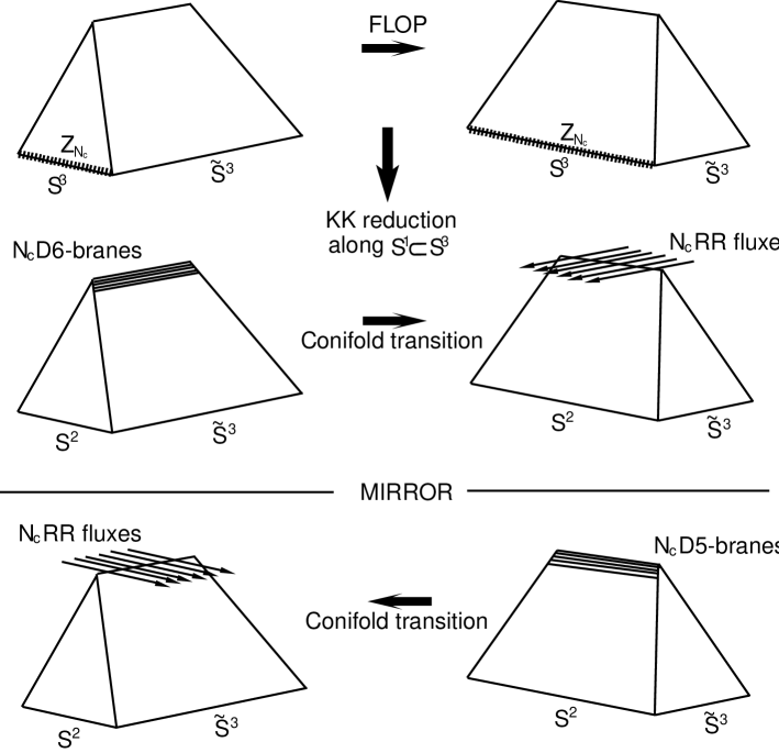
Figure 3: The flop transition in the $G_{2}$ manifold amounts to exchanging the rôle of the spheres. The action of $\mathbb{Z}_{N_{c}}\subset S^{1}\subset S^{3}$ is singular/regular on the left/right hand side of the upper figure. Corresponding quotients of the $S^{3}\in G_{2}$ give a singular manifold (upper left) which is an $A_{N_{c}-1}$ singularity fibered over $\tilde{S}^{3}$ that, when KK reduced along the $S^{1}$ represents $N_{c}$ D6-branes wrapping a sLag 3-cycle in the cotangent bundle $T^{*}\tilde{S}^{3}$ (middle left). RG flow towards the IR drives the system into the flop transition to a smooth $G_{2}$ manifold (upper right) or, from the 10d point of view, the system undergoes a conifold transition such that D6-branes dissapear and are replaced by RR fluxes through the exceptional $\mathbb{P}^{1}$ of the manifold $\mathcal{O}(-1)+\mathcal{O}(-1)\to\mathbb{P}^{1}$ (middle right). There is a mirror version of this story, in type IIB string theory, where $N_{c}$ D5-branes wrapping an holomorphic 2-cycle in $\mathcal{O}(-1)+\mathcal{O}(-1)\to\mathbb{P}^{1}$ are dual to $N_{c}$ fluxes through the sLag 3-cycle of the deformed conifold.

The resulting geometry in eleven dimensions is asymptotically conical. As such, it can be seen as the uplift of the system of wrapped D6–branes for an infinite value of the string coupling. Remind that the latter is related to the asymptotical value of the exponential of the dilaton which, in turn, is interpreted as the radius of the eleventh dimension. It should be possible to find a supergravity dual of this system with a finite radius circle at infinity, thus representing a string theory configuration at finite coupling. Indeed, a solution with the desired behaviour was found, and its uses in the context of the gauge/gravity duality were thoroughly studied [30].

3.6 The Maldacena–Núñez setup

There is an analogous setup in type IIB superstring theory that was proposed before the previous one by Maldacena and Núñez [106]. Roughly speaking, it can be thought of as the mirrored version of the type IIA scenario discussed before, as schematically displayed in Fig.3. It is actually simpler to tackle the problem in type IIB because it lacks the subtleties related to world-sheet instantons that affect the calculus of $\mathcal{N}=1$ superpotential terms. Again, we might start by drawing attention to an entry in the table of special holonomy manifolds that says that there are holomorphic $2$–cycles in a Calabi–Yau manifold where we can wrap D5–branes while preserving some supersymmetry. Recalling the discussion about flat D5–branes, we can already see that this system will be similar to $\mathcal{N}=1$ supersymmetric Yang–Mills theory in the IR but its UV completion will be given by a conformal 6d theory constructed on a stack of flat NS5–branes. We will not discuss this point here.

Consider a system of D5–branes wrapped on a supersymmetric $2$–cycle inside a Calabi–Yau threefold. The $R$–symmetry group is $SO(4)_{R}=SU(2)_{1}\times SU(2)_{2}$. We need to choose an $SO(2)$ subgroup in order to perform the twist and cancel the contribution of the spin connection in $S^{2}$. There are several options. The right twist to get $\mathcal{N}=1$ supersymmetric Yang–Mills is performed by identifying $SO(2)_{S^{2}}$ and $SO(2)\subset SU(2)_{1}$ (notice that $SO(2)\subset SU(2)_{2}$ is the same; other nontrivial options involve both $SU(2)$ factors). We can mimic the arguments given in the previous section. The fields on the D5–branes transform under $SO(1,5)\times SO(4)_{R}=SO(1,5)\times SU(2)_{1}\times SU(2)_{2}$ as $({\bf 4^{+}},{\bf 2})$ and $({\bf 4^{-}},{\bf 2})$ for the fermions (the $\pm$ superscripts correspond to chirality), $({\bf 1},{\bf 4})$ for the scalars and the gauge field remains a singlet under $R$–symmetry. When we wrap the D5–branes on a two–cycle, the symmetry group splits as $SO(1,3)\times SO(2)\times SU(2)_{1}\times SU(2)_{2}$. The corresponding representation for the fermions become $({\bf 2},{\bf+1},{\bf 2},{\bf 1})$, $({\bf\bar{2}},{\bf-1},{\bf 2},{\bf 1})$, $({\bf\bar{2}},{\bf+1},{\bf 1},{\bf 2})$ and $({\bf 2},{\bf-1},{\bf 1},{\bf 2})$, while the scalars transform in the $({\bf 1},{\bf 0},{\bf 2},{\bf 2})$. The effect of the twist is to preserve those fields which are uncharged under the diagonal group $SO(2)_{\rm diag}$ or, better, $U(1)_{\rm diag}$. Again, they are exactly the field content of the vector multiplet in $\mathcal{N}=1$ supersymmetric gauge theory in four dimensions: the gauge field and the fermions transform under $SO(1,3)\times SO(2)_{D}$, respectively, in the $(\mathbf{4},\mathbf{1})$ and $(\mathbf{2},+)\oplus(\mathbf{\bar{2}},-)$ representations .

It is possible to follow the same steps that we pursued in the case of the D6–brane. The supergravity solution shall appear as an appropriate domain wall solution of 7d gauged supergravity with the needed twist. There is however a subtlety: by turning on the $U(1)$ gauge field corresponding to $SO(2)\subset SU(2)_{1}$, we get a singular solution. We can turn on other components of the $SU(2)$ gauge fields by keeping their UV behavior, where the perturbative degrees of freedom used to discuss the topological twist are the relevant ones. This is a specific feature that, as we will see in the last lecture, can be mapped to an extremely important IR phenomenon of $\mathcal{N}=1$ supersymmetric gauge theory: chiral symmetry breaking due to gaugino condensation. From the point of view of gauged supergravity, turning on other components of the $SU(2)$ gauge field amounts to a generalization of the twisting prescription that has been discussed in [56]. We don’t have time to comment on this point any further.

Instead of deriving the so-called Maldacena–Núñez (MN) solution (which was actually originally obtained in a different context by Chamseddine and Volkov [39]), we will just write it down following a notation that makes contact with the gauged supergravity approach. The gauge field is better presented in terms of the triplet of Maurer–Cartan 1-forms on $S^{2}$

$$\sigma_{1}=d\theta~{},~{}~{}~{}~{}~{}\sigma_{2}=\sin\theta d\varphi~{},~{}~{}~{}~{}~{}\sigma_{3}=\cos\theta d\varphi~{},$$ (96)

that obey the conditions $d\sigma_{i}=-\frac{1}{2}\epsilon_{ijk}\sigma_{j}\wedge\sigma_{j}$. It is given by:

$$A^{1}=-\frac{1}{2}a(\rho)~{}\sigma_{1}~{},~{}~{}~{}~{}~{}\,\,\,A^{2}=\frac{1}{2}a(\rho)~{}\sigma_{2}~{},~{}~{}~{}~{}~{}\,\,\,A^{3}=-\frac{1}{2}\sigma_{3}~{},$$ (97)

where, for future use, we write the explicit dependence of $a(\rho)$,

$$a(\rho)=\frac{2\rho}{\sinh(2\rho)}~{}.$$ (98)

If we take $a(\rho)$ to zero, the solution goes to the previously mentioned singular case (which is customarily called the Abelian MN solution). The string frame metric is

$$ds_{str}^{2}=dx_{1,3}^{2}+g_{s}N\alpha^{\prime}\bigg{(}d\rho^{2}+e^{2h(\rho)}(\sigma_{1}^{2}+\sigma_{2}^{2})+\frac{1}{4}\sum_{i}(w^{i}-A^{i})^{2}\bigg{)}~{},$$ (99)

where

$$e^{2h(\rho)}=\rho\coth(2\rho)-\frac{\rho^{2}}{\sinh^{2}(2\rho)}-\frac{1}{4}~{}.$$ (100)

As expected, the solution has a running dilaton

$$e^{2\Phi(\rho)}=\frac{\sinh 2\rho}{2e^{h(\rho)}}~{},$$ (101)

that behaves linearly at infinity. There is a RR 3–form flux sourced by the D5–branes whose explicit expression reads

$$F_{[3]}=g_{s}N\alpha^{\prime}\left[2\ (w^{1}-A^{1})\wedge(w^{2}-A^{2})\wedge(w^{3}-A^{3})-\sum_{i=1}^{3}F^{i}\wedge w^{i}\right]~{},$$ (102)

where the physical radial distance is $r=\sqrt{g_{s}N\alpha^{\prime}}\rho$ and $F^{i}=dA^{i}+\epsilon^{ijk}A^{j}\wedge A^{k}$, and $w^{i}$ are left-invariant one-forms parameterizing $S^{3}$ (see the Appendix). If we perform the 7d gauged supergravity analysis, it becomes clear that we are left with four supercharges. We will use this supergravity solution in Lecture V and show how it encapsulates field theory physics.

We wish to point out at this stage that several interesting scenarios involving D5–branes and NS5–branes wrapping supersymmetric cycles have been considered so far. Most notably, systems which are dual to pure $\mathcal{N}=2$ supersymmetric gauge theories in four [61, 24] and three [62] spacetime dimensions, as well as to $\mathcal{N}=1$ theories in 3d [125, 104].

3.7 Decoupling

There are two issues of decoupling when considering wrapped Dp–branes. One is the decoupling of Kaluza-Klein modes on the wrapped cycle and the other is the decoupling of higher worldvolume modes from the field theory in the ‘field theory limit’.

Let us first consider the Kaluza-Klein modes. The mass scale associated with the Kaluza-Klein modes should be

$$\Lambda_{\text{KK}}^{q}\equiv M_{\text{KK}}^{q}\sim\frac{1}{\text{Vol}\,\Sigma_{q}},$$ (103)

where $\Sigma_{q}$ is the $q$-cycle in the Calabi-Yau wrapped by the branes. There is no a priori reason to identify this cycle with any particular cycle in the dual (backreacted) geometry. When probed at energies above $\Lambda_{\text{KK}}$ the field theory will be $p+1$ dimensional. These field theories typically have a positive $\beta$-function so the dimensionless effective coupling will decrease as one decreases the energy scale. At energy scales comparable to $\Lambda_{\text{KK}}$ the field theory will become $p-q+1$ dimensional; in the above we have considered $p-q+1=4$ in order to make contact with QCD-like theories and we will continue to do so in this section. We know from (7) that the beta function is now negative, and the dimensionless effective coupling will increase until it hits the characteristic mass scale of the field theory generated through dimensional transmutation $\Lambda_{\text{QCD}}$ (see Fig.4).

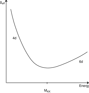
Figure 4: A plot of the effective coupling and its dependence on energy for the MN setup. The Kaluza-Klein scale $M_{KK}$ is the energy scale at which the wrapped dimensions become visible. Non-decoupling is the statement that $\Lambda_{QCD}$ is very close to $M_{KK}$.

This is the scale at which nonperturbative effects in the field theory become significant, and the scale at which we wish to study the gravity dual. It can be shown that for the gravity duals involving wrapped branes, it is not possible to decouple the two scales $\Lambda_{\text{QCD}}$ and $\Lambda_{\text{KK}}$. This can be shown in two ways, either by assuming some relations between certain cycles within the gravitational background with the initial cycle the D–branes wrap, as is often done in discussions of the Maldacena-Núñez background [25, 99] or by assuming that the gravitational background should not contain a regime dual to a weakly coupled field theory [69]. The study of strong coupling field theory via gravity duals would therefore, on general grounds, be contaminated by KK modes. This issue would be overcome, of course, provided suitable sigma models for a string theory in these background were found and their quantization carried out.

In spite of the precedent arguments, a further comment is in order at this point. In the context of supergravity duals corresponding to gauge theories with a global $U(1)\times U(1)$ symmetry, it has been recently shown that it is possible to perform a $\beta$–deformation (meaningly, an $SL(2,\mathbb{Z})$ transformation in the $\tau$ parameter of the corresponding torus in the gravity side) on both sides of the gauge/gravity duality [100]. In the particular case of the MN background, it has been argued that the resulting field theory is a dipole deformation of $\mathcal{N}=1$ supersymmetric Yang–Mills theory and that the deformation only affects the KK sector. It is then possible to render these states very massive, this possibly allowing to disentangle them from the dynamics [70] (see also [27]).

Let us now turn to study the gravitational modes. Supersymmetric Yang–Mills is not the complete field theory that describes the Dp–brane dynamics. The question at hand is whether there exists a limit, compatible with the other limits, that can be taken such that other degrees of freedom can be decoupled. We will not describe the arguments discussed in [85] and reviewed in [69] here in detail, but just mention that in the case of wrapped D5 and D6–branes it is again not possible to decouple gravitational modes and little-string theory modes respectively from $\Lambda_{QCD}$.

It is in a sense remarkable that, despite such problems with decoupling, dualities involving wrapped branes are able to reproduce so many features of ${\mathcal{N}}=1$ supersymmetric Yang–Mills theories. The study of $\beta$–deformed systems opens an avenue to KK decoupling [70] which might provide a clue to puzzle out this conundrum.

4 Lecture IV: D-branes at Singularities

In the previous lecture we introduced a framework to study the gravity dual of non-maximal supersymmetric gauge theories by wrapping Dp–branes, $p>3$ on calibrated cycles of special holonomy manifolds. Among the difficulties posed by this approach, we have seen that decoupling is far from being as clear as it is for D3–branes. If we insist on keeping D3–branes and want to deform the background, the simplest case amounts to considering orbifolds. Take for example, $\mathbb{C}^{2}/\mathbb{Z}_{2}$, where $\mathbb{Z}_{2}$ leaves invariant six coordinates of spacetime and acts nontrivially on the last four ones,

$$z^{1}=-z^{1}~{},~{}~{}~{}~{}~{}z^{2}=-z^{2}~{},$$ (104)

with $z^{1}=x^{6}+ix^{7}$ and $z^{2}=x^{8}+ix^{9}$. Now, take $\mathbb{R}^{1,9}\to\mathbb{R}^{1,5}\times\mathbb{R}^{4}\approx\mathbb{R}^{1,5}\times\mathbb{C}^{2}$ and consider how the action with the $\mathbb{Z}_{2}$ cyclic group affects the oscillators. Clearly,

$$\alpha_{n}^{r}\to-\alpha_{n}^{r}~{},\qquad\tilde{\alpha}_{n}^{r}\to-\tilde{\alpha}_{n}^{r}~{},\qquad\psi_{n}^{r}\to-\psi_{n}^{r}~{},\qquad\tilde{\psi}_{n}^{r}\to-\tilde{\psi}_{n}^{r}~{}.$$ (105)

We keep full control over perturbative string theory just by keeping states which are $\mathbb{Z}_{2}$–invariant. We now put flat D3–branes along the directions $0123$. If a D3–brane is not at the origin of the transverse space, it is not invariant under the action of $\mathbb{Z}_{2}$.

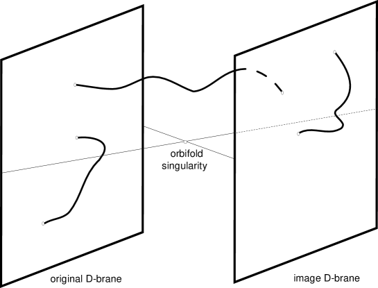
Figure 5: D–branes in presence of orbifold singularities and their image. There are open strings whose end points are on the D3–brane, on its image, and on both. The resulting gauge group is $U(1)\times U(1)$

We need to introduce an accompanying image to obtain a $\mathbb{Z}_{2}$–invariant state. Therefore, there will be open strings whose end points are placed only on the D3–brane, only on its image, and on both (see Fig.5). Correspondingly, the massless spectrum of this orbifold is $\mathcal{N}=2$ supersymmetric $U(1)\times U(1)$ with matter multiplets in the bifundamental representation with charges $(+1,-1)$ and $(-1,+1)$. Let us call them, in $\mathcal{N}=1$ notation, respectively $A_{i}$ and $B_{i}$. They are both doublets under the flavor (global) symmetry group $SU(2)\times SU(2)$. These theories are called quiver theories and their field content is represented by diagrams such as Fig.6. The number of supersymmetries is compatible with the fact that $\mathbb{C}^{2}/\mathbb{Z}_{2}$ orbifolds arise in the singular limit of $K3$. If we take the number of D3–branes to be $N_{c}$, the resulting theory will be $\mathcal{N}=2$ supersymmetric $U(N_{c})\times U(N_{c})$ with matter multiplets in the bifundamental with charges $(N_{c},\bar{N}_{c})$ and $(\bar{N}_{c},N_{c})$. One can compute the one-loop $\beta$–function and, given the fact that this theory has two $\mathcal{N}=2$ vector multiplets and two $\mathcal{N}=2$ matter hypermultiplets, it vanishes identically. The theory is conformal.

Consider now a D3–brane which is placed at the origin. There is no need to introduce an image. Such a brane is constrained to remain at the origin and, as such, the corresponding representation of the orbifold group is one dimensional. There are two such representations, the trivial one and the sign. The states that survive correspond to a single $\mathcal{N}=2$ vector multiplet: the scalars which parameterize the displacement away from the singularity and their superpartners are identically zero. In a sense, this is one half of the D3–brane which sits outside the origin. For this reason, it has been termed a fractional brane. It is immediate to see that its field content provides a nontrivial contribution to the $\beta$–function. Thus, when introducing fractional branes, we are dealing with nonconformal field theories.

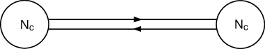
Figure 6: The quiver diagram representing a $SU(N_{c})\times SU(N_{c})$ supersymmetric gauge theory with adjoint vector fields and chiral bifundamental multiplets in $(N_{c},\bar{N}_{c})$ and $(\bar{N}_{c},N_{c})$ representations.

Let us make a couple of claims without discussing the details. It turns out that the orbifold singularity can be seen as the end of a shrinking process of a two cycle $\Sigma$: the inverse of a blowup. Indeed, a fractional brane can be interpreted as a D(p+2)–brane with two directions wrapping the exceptional cycle $\Sigma$ in the orbifold limit, where its geometrical volume vanishes. This would lead to a problem with the tensions if it wasn’t for the fact that the $B_{[2]}$ is such that $b=\int_{\Sigma}B=1/2$ is its only nonvanishing component and it is responsible for keeping the tension finite. Further support to this interpretation comes from the fact that the fractional Dp–brane couples to both $B_{\mu\nu}$ and $C_{[p+3]}$, as a D(p+2)–brane would do.

We would like to discuss in greater detail a case in which we have $\mathcal{N}=1$ supersymmetry. In order to do this we first need to introduce the conifold.

4.1 The Conifold

4.1.1 The Singular Conifold

The conifold, $\mathcal{Y}_{6}$, is a six dimensional (three complex dimensions) Calabi–Yau cone. It can be most easily introduced by considering its embedding in $\mathbb{C}^{4}$ given by the quadric

$$\mathcal{Y}_{6}\equiv\sum_{A=1}^{4}~{}(z^{A})^{2}=0~{},~{}~{}~{}~{}~{}~{}~{}z^{A}=x^{A}+iy^{A}~{}.$$ (106)

This is a smooth surface everywhere except at the point $z^{A}=0$ (which is a double point singularity: $\mathcal{Y}_{6}=0$, $d\mathcal{Y}_{6}=0$). Notice, moreover, that if $z^{A}\in\mathcal{Y}_{6}$, then $\lambda z^{A}\in\mathcal{Y}_{6}$ for any $\lambda\in\mathbb{C}$. Thus, the surface is made up of complex lines through the origin and, therefore, it is a cone. The apex of the cone is precisely the point $z^{A}=0$. The base of the cone, $\mathcal{X}_{5}$, is given by the intersection of the quadric with a sphere of radius $\rho$ in $\mathbb{C}^{4}$,

$$\mathcal{W}_{\rho}\equiv\sum_{A=1}^{4}~{}|z^{A}|^{2}=\rho^{2}~{}.$$ (107)

In terms of $x^{A}$ and $y^{A}$, this gives the following equations:

$$\vec{x}\cdot\vec{x}=\frac{1}{2}\rho^{2}~{},~{}~{}~{}~{}~{}\vec{y}\cdot\vec{y}=\frac{1}{2}\rho^{2}~{},~{}~{}~{}~{}~{}\vec{x}\cdot\vec{y}=0~{}.$$

The first equation defines an $S^{3}$ while the other two define an $S^{2}$ fibered over $S^{3}$. All such bundles are trivial, so the topology of the base of the cone is $S^{2}\times S^{3}$.

For some applications it is useful to define the matrix

$$W=\frac{1}{\sqrt{2}}z^{A}\sigma_{A}=\left(\begin{array}[]{cc}u&z\\ w&v\end{array}\right)\equiv\frac{1}{\sqrt{2}}\left(\begin{array}[]{cc}z^{3}+iz^{4}&z^{1}-iz^{2}\\ z^{1}+iz^{2}&-z^{3}+iz^{4}\end{array}\right)~{},$$ (108)

where $\sigma_{A}=(\sigma_{k},i\mathbb{I})$, $\sigma_{k}$ are the Pauli matrices. In terms of $W$ the quadric above can be immediately rewritten as

$$\det W=uv-wz=0~{}.$$ (109)

Notice that the sphere (107) can be cast in terms of $W$ as

$$Tr\,[W^{\dagger},W]=\rho^{2}~{}.$$ (110)

The existence of a Ricci-flat Kähler metric on $\mathcal{Y}_{6}$ implies that the base of the cone, $\mathcal{X}_{5}$, admits an Einstein metric. The simplest option (besides the trivial one given by $S^{5}$), and the only one that was known until very recently, is $\mathcal{X}_{5}=T^{1,1}$ whose Einstein metric is [37]

$$ds_{5}^{2}\,(T^{1,1})=\frac{1}{9}\,\left(d\tilde{\psi}+\sum_{i=1}^{2}\cos\theta_{i}\,d\phi_{i}\right)^{2}+\frac{1}{6}\sum_{i=1}^{2}(d\theta_{i}^{2}+\sin^{2}\theta_{i}d\phi_{i}^{2})~{},$$ (111)

where $0\leq\theta_{i}<\pi$, $0\leq\phi_{i}<2\pi$ and $0\leq\tilde{\psi}<4\pi$. This is not the induced metric coming from the defining embedding in $\mathbb{C}^{4}$ (which is not, indeed, Ricci flat). The isometry group of $T^{1,1}$ is $SU(2)\times SU(2)\times U(1)$. Moreover, the metric makes evident that $T^{1,1}$ is a $U(1)$ fibration over a Kähler–Einstein manifold, $S^{2}\times S^{2}$. It is compact and homogeneous,

$$T^{1,1}=\frac{SU(2)\times SU(2)}{U(1)}~{}.$$ (112)

The singular conifold (or simply conifold) metric is the metric of a cone over $T^{1,1}$:

$$ds_{6}^{2}(\mathcal{Y}_{6})\,=\,d\rho^{2}\,+\,\rho^{2}\,ds_{5}^{2}\,(T^{1,1})~{}.$$ (113)

We write in the Appendix a set of useful formulas that should clarify some of the computations in the remaining of this section.

4.1.2 The Deformed Conifold

How can we resolve the singularity at the apex?. The most natural way seems to add a non–vanishing r.h.s. to the quadric

$$\mathcal{Y}_{6}^{\mu}\equiv\sum_{A=1}^{4}(z^{A})^{2}=\mu^{2}~{},$$ (114)

or, in terms of the matrix $W$,

$$\det W=uv-wz=-\frac{1}{2}\mu^{2}~{}.$$ (115)

This is the deformation of the conifold: at the apex, the $S^{3}$ remains finite while the $S^{2}$ shrinks. The appearance of $\mu\neq 0$ breaks a $U(1)$ invariance $z^{A}\to e^{i\alpha}z^{A}$ to a discrete subgroup $\mathbb{Z}_{2}$. This will be interpreted as the realization of chiral symmetry breaking at the IR as seen from geometry.

4.1.3 The Resolved Conifold

Another way of getting rid of the singular point is by the standard blowup procedure. By definition, this amounts to considering the same manifold and replacing a point, in this case the apex of the cone, by a projective sphere. This is done as follows. Consider the defining equation for the conifold (109). Now, replace this equation by

$$\begin{pmatrix}u&&z\cr w&&v\end{pmatrix}~{}\begin{pmatrix}\lambda_{1}\cr\lambda_{2}\end{pmatrix}=0~{},$$ (116)

where $\lambda_{1},\lambda_{2}\in\mathbb{C}$ and they cannot both be zero. Only at the apex, $\lambda_{1}/\lambda_{2}$ is unconstrained, so one has an entire  $\mathbb{P}^{1}=S^{2}$. This defines what is called the small resolution of the conifold: at the apex, $S^{2}$ is finite while $S^{3}$ shrinks.

Figure 7: Different resolutions of the conifold correspond to either the $S^{3}$ (deformed) or the $S^{2}$ (resolved) being non-vanishing at the origin. The resolution parameter will appear as an additional parameter in the metrics for these two cases.

Ricci-flat Kähler metrics on these manifolds, compatible with $ds_{6}^{2}(\mathcal{Y}_{6})$ are known. They have the same asymptotics as the singular conifold and differ only in the region near the tip of the cone (the IR of the dual field theory). Both the metric of the conifold, as well as those of its resolution and its deformation, can be found by considering the uplift to eleven dimensions of $D6$–branes wrapping a 2-cycle in a Calabi–Yau manifold [53, 57].

Let us finally comment on the fact that this manifold is also called $\mathcal{O}(-1)+\mathcal{O}(-1)\to\mathbb{P}^{1}$. This means that it can be constructed by taking two copies of $\mathbb{C}^{3}$ with coordinates $(x,u,z)$ and $(x^{\prime},u^{\prime},z^{\prime})$, identifying $z$ (respectively $z^{\prime}$) as the coordinate of the northern (southern) hemisphere of the $\mathbb{P}^{1}$, and finally gluing the two copies of $\mathbb{C}^{3}$ with the identification:

$$z^{\prime}=\frac{1}{z}~{},\qquad x^{\prime}=xz~{},\qquad u^{\prime}=uz~{}.$$ (117)

4.2 The Klebanov–Witten setup

(dual to $\mathcal{N}=1$, $SU(N)\times SU(N)$ superconformal Yang-Mills with bi-fundamental matter)

Consider now the addition of a stack of flat D3–branes at the apex of the conifold. It is not difficult to write down the corresponding supergravity solution [92]:

$$ds_{10}^{2}=h(r)^{-\frac{1}{2}}(dx_{i})^{2}+h(r)^{\frac{1}{2}}\left(dr^{2}+r^{2}ds_{T^{1,1}}^{2}\right)~{},$$ (118)

where

$$h(r)=1+\frac{L^{4}}{r^{4}}~{},\qquad L^{4}=4\pi g_{s}N(\alpha^{\prime})^{2}~{},$$ (119)

as in the case of flat D3–branes presented in section 2 and the Einstein metric on $T^{1,1}$ is given in the appendix. Clearly, the near horizon limit of (118) is just given by the direct product $AdS_{5}\times T^{1,1}$. This is a particular example of the more general statement that the gravity dual to the field theory living on D3–branes placed at a conifold singularity is $AdS_{5}\times X_{5}$, where $X_{5}$ is the Einstein manifold which is the base of the cone [68]. The $AdS_{5}$ factor in the metric is telling us that the gauge theory has a conformal fixed point. The number of supersymmetries can be deduced from the holonomy of the background. It leads to four supercharges which are doubled by the presence of a conformal symmetry.

In summary, the resulting theory is $\mathcal{N}=1$ superconformal gauge theory. The $U(1)$ isometry corresponding to shifts in $\tilde{\psi}$ amounts to the $R$ symmetry while the $SU(2)\times SU(2)$ isometry corresponds to a global flavor symmetry. If we look at the defining equation of the conifold (109), we see that this equation is automatically satisfied if we write

$$u=A_{1}B_{1}~{},~{}~{}~{}v=A_{2}B_{2}~{},~{}~{}~{}z=A_{1}B_{2}~{},~{}~{}~{}w=A_{2}B_{1}~{}.$$ (120)

The defining equation of the manifold is related to the moduli space of the gauge theory. Thus, the theory can be thought of as having constituents $A_{i}$ and $B_{i}$ (in presence of $N$ D3–branes they have to be promoted to matrix-valued bifundamental chiral fields of the gauge group $SU(N)\times SU(N)$ transforming, respectively, in the $({\bf N},{\bf\bar{N}})$ and $({\bf\bar{N}},{\bf N})$ representations. Besides, $A_{i}$ is a doublet of the first $SU(2)$ (and a singlet of the second) and, conversely, $B_{i}$ is the other way around. The dual superconformal gauge theory can be represented by a quiver diagram. The only ingredient that is still lacking is the superpotential. Taking into account the fact that the superpotential has $R$ charge equal to two and it is a singlet under flavor symmetries, it has to be of the form [92]

$$W=\epsilon^{ij}\epsilon^{kl}TrA_{i}B_{k}A_{j}B_{l}~{}.$$ (121)

Indeed, the $A_{i}$ and $B_{i}$ fields have $R$ charge equal to $\frac{1}{2}$, conformal dimension $\frac{3}{4}$ and, respectively, baryon number equal to $+1$ and $-1$.

4.3 Klebanov–Tseytlin solution

(the UV of $\mathcal{N}=1$, $SU(N+M)\times SU(N)$ supersymmetric Yang–Mills theory with bi-fundamental matter)

If we add fractional branes into the picture, conformal symmetry will be immediately spoiled. The solution to this system was originally developed in Refs.[88, 91]. Let us consider a set up in which, in addition to the metric and a RR 5-form, we switch on the RR 3-form $F_{3}$. We keep the metric ansatz

$$ds_{10}^{2}=h(r)^{-\frac{1}{2}}(dx_{i})^{2}+h(r)^{\frac{1}{2}}\left(dr^{2}+r^{2}ds_{T^{1,1}}^{2}\right)~{},$$ (122)

where $h(r)$ is now a function to be determined. In order to make an ansatz for $F_{3}$, we can make use of the closed 3-form of the conifold $w_{3}$ (see Appendix B). We can make the following ansatz,

$$F_{3}=fw_{3}~{},$$ (123)

where $f$ still has to be determined. We will fix $f$ by means of the quantization condition corresponding to a stack of D5-branes. Taking $\star F^{(7)}=F_{3}$, we have

$$\int_{S^{3}}F_{3}=4\pi^{2}\alpha^{\prime}~{}M~{},~{}~{}~{}~{}~{}M\in\mathbb{Z}~{},$$ (124)

$M$ being the number of D5-branes and $S^{3}$ the sphere which is given by the set of $T^{1,1}$ with $\theta_{2}=\phi_{2}=0$. These D5-branes are wrapped on a (supersymmetric) 2-cycle and, thus, we are going to have $N$ D3-branes and $M$ fractional D3-branes. From equations (123) and (124), we get $f=\frac{M}{2}\alpha^{\prime}$, and

$$F_{3}=\frac{M}{2}\alpha^{\prime}~{}w_{3}~{},$$ (125)

First of all, it is clear that $dF_{3}=0$ is automatic. Since $dF_{5}\neq 0$, we must also switch on a NSNS 3-form $H_{3}=dB$. In order to construct the appropriate NSNS 2-form potential $B$, we make use of the closed 2-form of the conifold $w_{2}$. Let us take

$$B=T(r)\,w_{2}~{},~{}~{}~{}\Rightarrow~{}~{}~{}H_{3}=T^{\prime}(r)\,dr{\wedge}w_{2}~{},$$ (126)

where $T(r)$ is to be determined. Plugging in these expressions into $dF_{5}=H_{3}\wedge F_{3}$, we can write $T(r)$ as

$$(r^{5}h^{\prime}(r))^{\prime}=-27MT^{\prime}(r)\alpha^{\prime}g_{s}~{}.$$ (127)

Now, given that $F_{1}=0$ in this background, the dilaton equation of motion reads

$$\nabla^{2}\Phi=\frac{g_{s}}{12}\left(e^{\Phi}F_{3}^{2}-e^{-\Phi}H_{3}^{2}\right)~{}.$$ (128)

Thus, for a constant dilaton $e^{\Phi}=g_{s}$, we must have

$$g_{s}^{2}F_{3}^{2}=H_{3}^{2}~{}.$$ (129)

From this equation we can derive an explicit expression for $T^{\prime}(r)$ such that

$$H_{3}=\frac{3g_{s}M}{2r}\alpha^{\prime}~{}dr{\wedge}w_{2}\,,\qquad B_{2}=\frac{3g_{s}M}{2}\log\frac{r}{r_{0}}\alpha^{\prime}w_{2}~{}.$$ (130)

Then

$$H_{3}{\wedge}F_{3}=\frac{3g_{s}M^{2}}{4r}(\alpha^{\prime})^{2}~{}dr{\wedge}w_{2}{\wedge}w_{3}~{}.$$ (131)

Using Eq.(220), we can readily see that

$$F_{3}^{2}=\frac{3^{5}M^{2}}{r^{6}}(\alpha^{\prime})^{2}h^{-3/2}~{}.$$ (132)

Using this solution for $T^{\prime}(r)$, we can compute $h(r)$. A first integral of the equation above is easy to perform,

$$r^{5}h^{\prime}(r)=-\frac{81}{2}M^{2}g_{s}^{2}(\alpha^{\prime})^{2}\log r+{\it const}~{}.$$ (133)

This equation can be integrated to be

$$h(r)=\frac{81M^{2}g_{s}^{2}(\alpha^{\prime})^{2}}{2}\left(\frac{\log r}{4r^{4}}+\frac{1}{16r^{4}}\right)+\frac{\it const}{r^{4}}+{\it const^{\prime}}$$ (134)

In the near-horizon limit we can drop the additive constant. Thus

$$h(r)=\frac{27\pi(\alpha^{\prime})^{2}}{4r^{4}}\left(g_{s}N+a(g_{s}M)^{2}\log\frac{r}{r_{0}}+\frac{a}{4}(g_{s}M)^{2}\right)~{},$$ (135)

with $a=\frac{3}{2\pi}$. It is convenient to define at this point

$$N_{eff}=N+\frac{3}{2\pi}g_{s}M^{2}\log\frac{r}{r_{0}}~{},$$ (136)

such that, for example,

$$r^{5}h^{\prime}(r)=-27\pi(\alpha^{\prime})^{2}g_{s}N_{eff}~{},$$ (137)

and the RR 5-form becomes

$$g_{s}F_{5}=27\pi(\alpha^{\prime})^{2}g_{s}N_{eff}dVol(T^{1,1})+{\rm Hodgedual}~{}.$$ (138)

From this formula it can be deduced

$$\int_{T^{1,1}}F_{5}=(4\pi^{2}\alpha^{\prime})^{2}N_{eff}~{}.$$ (139)

Notice that $N_{eff}$ is a logarithmically running number of colors.

4.3.1 The Running of $N_{eff}$ and Seiberg Duality

The gauge couplings of the two gauge groups are given by [92]

$$\frac{1}{g_{1}^{2}}+\frac{1}{g_{2}^{2}}\approx e^{-\Phi}~{},\qquad\frac{1}{g_{1}^{2}}-\frac{1}{g_{2}^{2}}\approx e^{-\Phi}\left(\int_{S^{2}}B_{2}-\frac{1}{2}\right)~{},$$ (140)

and we recall that we are considering a constant dilaton $\Phi$. Equation (130) then shows that $1/g_{1}^{2}$ and $1/g_{2}^{2}$ run logarithmically in different directions. If we think of the RG flow in the $SU(N+M)\times SU(N)$ theory, it is not difficult to see that there exists a scale (value of $r$, say, $\Lambda_{N+M}$) at which the gauge coupling corresponding to the first factor, $g_{1}$, diverges. To go beyond this scale we must perform a Seiberg duality. This is an S–duality statement telling us that an $\mathcal{N}=1$ supersymmetric gauge theory with gauge group $SU(N_{c})$ and $N_{f}$ flavors, when strongly coupled, is dual to a weakly coupled $SU(N_{f}-N_{c})$ theory with $N_{f}$ flavors, provided $\frac{3}{2}N_{c}<N_{f}<3N_{c}$. Thus, at a scale given by $\Lambda_{N+M}$, given that $N_{c}=N+M$ and $N_{f}=2N$ for the first factor, $SU(N+M)\to SU(N-M)$ under Seiberg duality. The solution we presented above has a cascade of such dualities

$$SU(N+M)\times SU(N)\rightarrow SU(N)\times SU(N-M)\rightarrow SU(N-M)\times SU(N-2M)\rightarrow\dots$$ (141)

in which, at decreasing energy scales, the coupling of the first gauge group diverges, and we can think of performing a Seiberg duality on that factor.

The cascade of Seiberg dualities is encoded in the supergravity background that we have presented above in the logarithmic running of $N_{eff}$ (136). There becomes a point where the effective number of colors vanishes and the solution can be shown to be singular. The way to obtain a well behaved supergravity solution valid in the infrared was presented in [90], and is related to the deformed conifold which we presented in section 4.1.2. We come to this point in what follows.

4.4 The Klebanov–Strassler setup

(dual to $\mathcal{N}=1$, $SU(N+M)\times SU(N)$ supersymmetric Yang-Mills theory with bi-fundamental matter)

We would like to deform the conifold such that the RG flow leads to a duality cascade that ends at the IR. Let us consider an ansatz for the 10d line element similar to the ones above

$$ds^{2}=h^{-1/2}(\tau)dx_{1,3}^{2}+h^{1/2}(\tau)ds_{6}^{2}~{},$$ (142)

where now however $ds_{6}^{2}$ is the metric of the deformed conifold (see the Appendix for further details),

$$ds_{6}^{2} = \frac{1}{2}\epsilon^{4/3}K(\tau)\bigg{[}\frac{1}{3K(\tau)^{2}}(d\tau^{2}+(g^{5})^{2})+\sinh^{2}(\tau/2)((g^{1})^{2}+(g^{2})^{2})$$ (144)

$$~{}~{}~{}~{}~{}~{}~{}~{}~{}~{}~{}~{}~{}~{}~{}~{}~{}~{}~{}~{}~{}~{}+\cosh^{2}(\tau/2)\,((g^{3})^{2}+(g^{4})^{2})\bigg{]}~{},$$

the function $K(\tau)$ being given by the following expression

$$K(\tau)=\frac{(\sinh 2\tau-2\tau)^{1/3}}{2^{1/3}\sinh\tau}~{}.$$ (145)

Notice that this function has a finite nonvanishing limiting value when $\tau$ goes to zero,

$$\lim_{\tau\to 0}K(\tau)=\left(\frac{2}{3}\right)^{1/3}~{}.$$ (146)

For this reason, it is clear that there is a $S^{2}$ (spanned by $g^{1}$ and $g^{2}$) that shrinks to zero volume at $\tau=0$ while there is a finite $S^{3}$.

This finite $S^{3}$ presents one argument in favor of this idea. The divergence in the KT solution could be shown to arise from an infinite energy density in $F_{3}^{2}$, due to the fact that as the flux of $F_{3}$ through the $S_{3}$ is constant and equal to $M$, when the $S^{3}$ collapses, $F_{3}$ must diverge. A more rigorous justification involves studying the moduli space of the field theory and showing that it is in fact given by the deformed conifold (115) when the nonperturbative contributions to the superpotential are considered [6].

The derivation of the solution is involved and follows similar steps to the ones presented above for the KT case. The solution is more complicated and we present it now.

The fields are

$$g_{s}F_{5} = d^{4}x{\wedge}dh^{-1}+{\rm Hodge~{}dual}=\frac{g_{s}^{2}M^{2}(\alpha^{\prime})^{2}}{4}\ell(\tau)g^{1}{\wedge}\dots\wedge g^{5}+{\rm Hodge~{}dual}$$

$$F_{3} = \frac{M\alpha^{\prime}}{2}\left[(1-F)g^{3}{\wedge}g^{4}{\wedge}g^{5}+Fg^{1}{\wedge}g^{2}{\wedge}g^{5}+F^{\prime}d\tau{\wedge}(g^{1}{\wedge}g^{3}+g^{2}{\wedge}g^{4})\right]$$

$$B = \frac{g_{s}M\alpha^{\prime}}{2}\left(f(\tau)g^{1}\wedge g^{2}+K(\tau)g^{3}\wedge g^{4}\right)$$

$$H_{3} = \frac{g_{s}M\alpha^{\prime}}{2}\left[d\tau{\wedge}(f^{\prime}g^{1}{\wedge}g^{2}+K^{\prime}g^{3}{\wedge}g^{4})+\frac{1}{2}(K-f)g^{5}{\wedge}(g^{1}{\wedge}g^{3}+g^{2}{\wedge}g^{4})\right]\,.$$ (147)

The equations of motion can be solved and the above functions are found to be

$$F(\tau) = \frac{\sinh\tau-\tau}{2\sinh\tau}\,,$$

$$h(\tau) = \frac{2^{2/3}\alpha}{4}\int_{\tau}^{\infty}dx\frac{x\coth x-1}{\sinh^{2}x}(\sinh 2x-2x)^{1/3}\,,$$

$$f(\tau) = \frac{\tau\coth\tau-1}{2\sinh\tau}(\cosh\tau-1)\,,$$

$$l(\tau) = \frac{\tau\coth\tau-1}{4\sinh^{2}\tau}(\sinh 2\tau-2\tau)\,,$$ (148)

where

$$\alpha=4g_{s}^{2}M^{2}(\alpha^{\prime})^{2}\epsilon^{-8/3}\,.$$ (149)

This solution has the same UV (large $r$) behavior as the KT solution presented above, but is non-singular in the IR (small $r$).

5 Lecture V: Nonperturbative phenomena as seen from supergravity

Let us end these lectures by providing a summary of several nonperturbative phenomena in $\mathcal{N}=1$ supersymmetric gauge theory as seen from the supergravity side of the duality. We will go over those phenomena presented in lecture I and discuss the way this information is encoded in the dual supergravity description. We will mostly work within the framework given by the MN solution in type IIB.

5.1 Chiral symmetry breaking

Chiral symmetry breaking is the phenomenom by which the $U(1)_{A}$ mentioned in (3) gets broken to a discrete subgroup:

$$U(1)_{A}\rightarrow\mathbb{Z}_{2N_{c}}\,.$$ (150)

In field theory this is known to be a UV effect caused by instantons.

We know from probe brane analysis the specific relations between the gauge coupling and $\theta$–angle in the gauge theory and supergravity fields. In the case of $N_{c}$ D5–branes wrapping a two–cycle $\Sigma$ inside a Calabi–Yau, they read:

$$\frac{4\pi}{g_{YM}^{2}} = \frac{1}{(2\pi l_{s})^{2}g_{s}}\int_{\Sigma}d^{2}\xi\ e^{-\Phi}\sqrt{\det G}~{},$$ (151)

$$\frac{\theta_{YM}}{2\pi} = \frac{1}{(2\pi l_{s})^{2}g_{s}}\int_{\Sigma}C_{[2]}~{},$$ (152)

where $G$ and $C_{[2]}$ are space-time fields restricted to the cycle. The two-cycle is non-trivially embedded in the geometry [23]. Using the formulas corresponding to the MN background, we can explicitly compute

$$\frac{4\pi}{g_{YM}^{2}} = \frac{N_{c}}{4\pi}\left(e^{2h(\rho)}+(a(\rho)-1)^{2}\right)=\frac{N_{c}}{\pi}\ \rho\tanh\rho~{},$$ (153)

$$\frac{\theta_{YM}}{2\pi} = \frac{N_{c}}{2\pi}~{}\psi_{0}~{},$$ (154)

where $\psi_{0}$ is an integration constant that, due to the embedding, gets fixed to $0$ or $2\pi$.

The $U(1)$ $R$–symmetry in the gauge theory has to do with shifts in the angular variable $\psi$ in supergravity. At the UV, we can approach the solution by the Abelian (singular) one because $a(\rho)\to 0$ when $\rho\to\infty$. Then, using the value of $C_{[2]}$ in the Abelian solution,

$$\frac{\theta_{YM}}{2\pi}=\frac{1}{(2\pi l_{s})^{2}g_{s}}\int_{\Sigma}C_{[2]}\approx\frac{N_{c}}{2\pi}(\psi+\psi_{0})~{},$$ (155)

which is clearly invariant under ($\theta_{YM}\to\theta_{YM}+2\pi k$)

$$\psi\to\psi+\frac{2\pi k}{N_{c}}~{}.$$ (156)

Since an $R$–symmetry transformation of parameter $\epsilon$ changes the $\theta$–angle by $\theta_{YM}\to\theta_{YM}-2N_{c}\epsilon$, it translates to $\psi\to\psi+2\epsilon$. This means that the remaining UV symmetry corresponds to $U(1)_{R}\to\mathbb{Z}_{2N_{c}}$ which is a well-known instanton effect in the gauge theory: this is nothing other than the chiral anomaly, a one–loop effect that is an UV phenomenon. The holographic dual of this feature is well understood [89]. The value of $\theta_{YM}$ in the complete solution tells us that $\mathbb{Z}_{2N_{c}}\to\mathbb{Z}_{2}$ in the IR, as can be seen, for example, in equation (154). Notice that, in a sense, it is the non-vanishing value of $a(\rho)$ which is somehow responsible for encoding the IR effects of the gauge theory dual. Let us discuss this aspect in greater detail in the following section.

Before proceeding though, let us mention the effect in the gravity picture which is dual to chiral symmetry breaking in the field theory. This was first studied by [89] in the KS background. Fluctuations $\psi\rightarrow\psi+\lambda$ about the $U(1)$ isometric direction of the metric with coordinate $\psi$ where described by a vector in terms of a vector field $A_{i}$. Even though the direction is an isometry, when taking into account the contribution from the RR potentials, it was found that the effective action for the fluctuation corresponds to the action of a massive (and gauge invariant) vector field $W_{i}=A_{i}+\partial_{i}\lambda$. These fluctuations are dual to the chiral symmetry current, and hence the anomaly in the field theory arises as a Higgs’ effect in the gravity dual. Correlators involving the chiral current in this picture were studied in [95, 96]. The effect was also studied in the IIA gravity duals and their M theory uplifts [69]. The subtlety in this context involves the fact that as already mentioned, the IIA gravity duals lift to pure geometry in M theory, therefore fluctuations dual to the chiral current can no longer be around a $U(1)$ isometry.

More on chiral symmetry breaking in the context of AdS/CFT as applied to confining theories can be found in [13, 21, 22].

5.2 Gaugino Condensation

We have seen that the supergravity solution nicely accounts for the chiral symmetry breaking phenomenon. The IR effects can be traced to the appearance of the function $a(\rho)$ in the solution. In the gauge theory side we know that the IR breaking $\mathbb{Z}_{2N_{c}}\to\mathbb{Z}_{2}$ is a consequence of gaugino condensation. Thus, it seems natural to identify $<\lambda\lambda>$ with $a(\rho)$ in a way that we would explore in what follows. Let us first give further arguments to support this claim. From the second order equation that is obeyed by the funcion $a(\rho)$,

$$\left(e^{-4h(\rho)-2\Phi(\rho)}a^{\prime}(\rho)\right)^{\prime}=e^{2h(\rho)-6\Phi(\rho)}~{}a(\rho)~{}(a(\rho)^{2}-1)~{},$$ (157)

we can extract the asymptotic behavior of the solution. Following the discussion in the original Maldacena’s setup, we need the asymptotic value of $a(\rho)$ for both linearly independent solutions,

$$a(\rho)\to a_{d}(\rho)=\frac{1}{\sqrt{\rho}}~{},~{}~{}~{}~{}~{}{\rm and}~{}~{}~{}~{}~{}a(\rho)\to a_{sd}(\rho)=2\rho\,e^{-2\rho}~{}.$$ (158)

where the subindices mean, respectively, dominant and sub-dominant. The former is a normalizable solution while the latter is non-normalizable. If we blindly apply the AdS/CFT and holographic RG flow prescriptions, we can see that the dominant solution corresponds to the insertion of the operator $<\bar{\lambda}\lambda>$. This is a mass term for the gaugino which breaks supersymmetry. In turn, the sub-dominant solution –which actually corresponds to the behavior in the MN background–, is giving a vacuum expectation value to the operator $<\lambda\lambda>$. Thus, the gaugino condensate is related to $a(\rho)$ [9].

The gaugino condensate is a protected operator in the gauge theory, which is related to the dynamical scale via $\langle\rm Tr~{}\lambda\lambda\rangle\approx\Lambda_{QCD}^{3}$. Notice that, due to this issue, the identification between $a(\rho)$ and the gaugino condensate should be an exact equation. We still need to introduce the subtraction scale $\mu$ of the gauge theory. Taking into account mass units and the precedent arguments, it seems natural to identify [48]

$$\mu^{3}\ a(\rho)=\Lambda_{QCD}^{3}~{}.$$ (159)

Namely,

$$\frac{\Lambda_{QCD}^{3}}{\mu^{3}}=\frac{2\rho}{\sinh 2\rho}~{}.$$ (160)

This relation gives implicitly the energy/radius relation between supergravity coordinates and gauge theory scales. A final comment is in order. The function $a(\rho)$ is responsible for regularizing the otherwise singular Abelian MN background. It is interesting to point out that this relation between the last step of chiral symmetry breaking and space-time singularity resolution is also present in Klebanov-Strassler’s setup [90]. There, gaugino condensation and chiral symmetry breaking arise as a consequence of the deformation of the conifold singularity.

5.3 The Beta Function

Recall the definition of the $\beta$–function. It encodes the variation of the gauge coupling constant with energy,

$$\beta(g_{YM})=\frac{\partial g_{YM}}{\partial\ln\frac{\mu}{\Lambda_{QCD}}}~{}.$$ (161)

Taking into account the radial dependence of all quantities involved in this expression, we can write

$$\beta(g_{YM})=\frac{\partial g_{YM}}{\partial\rho}\frac{\partial\rho}{\partial\ln\frac{\mu}{\Lambda_{QCD}}}~{}.$$ (162)

Let us first use the asymptotic behavior, neglecting subleading exponential corrections. The leading contribution to the Yang–Mills coupling is linear,

$$\frac{4\pi}{g_{YM}^{2}}\approx\frac{N_{c}}{\pi}~{}\rho~{}.$$ (163)

We therefore get:

$$\frac{\partial g_{YM}}{\partial\rho}\approx\frac{\pi}{\sqrt{N_{c}}}\rho^{-3/2}\approx-\frac{N_{c}g_{YM}^{3}}{8\pi^{2}}~{}.$$ (164)

On the other hand, we can compute from equation (162),

$$\frac{\partial\rho}{\partial\ln\frac{\mu}{\Lambda_{QCD}}}\approx\frac{3}{2}\left(1-\frac{1}{2\rho}\right)^{-1}\approx\frac{3}{2}\left(1-\frac{N_{c}g_{YM}^{2}}{8\pi^{2}}\right)^{-1}~{},$$ (165)

where we used the asymptotic relation in the last step to trade $\rho$ for $g_{YM}$. Putting together these results, we obtain

$$\beta(g_{YM})=-\frac{3N_{c}g_{YM}^{2}}{16\pi^{2}}\left(1-\frac{N_{c}g_{YM}^{2}}{8\pi^{2}}\right)^{-1}~{},$$ (166)

which is the correct NSVZ $\beta$-function at all-loops computed in the Pauli–Villars renormalization scheme for $\mathcal{N}=1$ supersymmetric Yang–Mills theory [112].

We can now work out the calculation using the complete solution, this resulting in the following expression for the $\beta$–function [48, 23, 110],

$$\beta(g_{YM})=-\frac{3N_{c}g_{YM}^{3}}{16\pi^{2}}\left(1-\frac{N_{c}g_{YM}}{8\pi^{2}}+\frac{2e^{-16\pi^{2}/N_{c}g_{YM}^{2}}}{1-e^{-16\pi^{2}/N_{c}g_{YM}^{2}}}\right)^{-1}~{}.$$ (167)

The last contribution seems to be originated in non-perturbative fractional instantons contributions to the running of the coupling. It is not yet understood what the origin of these configurations might be, and this formula for the $\beta$–function is still under debate. On the other hand, the result must be taken with care as it is unclear how to decouple the four-dimensional dynamics Kaluza–Klein modes on $\Sigma$ within the region of validity of supergravity.

5.4 Confinement and Screening of Magnetic Monopoles

A fundamental charge is described by a fundamental string extended along one of the gauge theory directions, say, $z$. The quark-antiquark potential $V_{q\bar{q}}$, then, is given by its Euclidean Nambu–Goto action,

$$S_{NG}=\frac{1}{2\pi\alpha^{\prime}}\int d\tau d\sigma\sqrt{-{\rm det}\,g_{ab}}~{},$$ (168)

where $g_{ab}$ is the pull-back of the string frame metric on the worldvolume of the string. It is an immediate consequence of the form of the metric in the MN solution that the string will prefer to stretch out sitting at $r=0$, where the value of $e^{\phi}$ is the least. Thus,

$$S_{NG}=\frac{e^{\phi_{0}}}{2\pi\alpha^{\prime}}\int dx\,dt\qquad\Rightarrow\qquad T_{q\bar{q}}=\frac{e^{\phi_{0}}}{2\pi\alpha^{\prime}}\neq 0~{}.$$ (169)

The string tension does not vanish and the theory is confining. If the same computation is performed in the $AdS_{5}\times S^{5}$ background, the result is zero, this reflecting the non-confining nature of $\mathcal{N}=4$ SYM theory. We will discuss confining strings in more detail in the next section. Let us conclude the present one by computing the monopole-antimonopole potential. Magnetic monopole sources correspond to D3–branes wrapping $S^{2}$ and extending along the radial direction. The potential $V_{m\bar{m}}$ then corresponds to the energy of a D3–brane wrapping $S^{2}$ and extending along a gauge theory direction. The D3–brane worldvolume coordinates are $(\tau,\sigma,\Theta,\Phi)$ and the embedding into the background geometry reads $t=\tau$, $x=\sigma$, $\theta=\Theta$, $\phi=\Phi$, and $r=r(\sigma)$. Then,

$$S_{NG} = \frac{1}{2\pi\alpha^{\prime}}\int d\tau\,d\sigma\,d\Theta\,d\Phi\,\sqrt{\det(-g)}$$ (170)

$$= 4\pi g_{s}N_{c}\int d\sigma\,e^{2\phi(r(\sigma))}\bigg{(}e^{2h(r(\sigma))}+\frac{(a(r(\sigma))-1)^{2}}{4}\bigg{)}\sqrt{1+\alpha^{\prime}g_{s}N_{c}(r^{\prime}(\sigma))^{2}}~{}.$$ (171)

But, as we have seen, the $S^{2}$ shrinks in the IR ($r\to 0$), this implying that the corresponding wrapped D3–branes become tensionless,

$$T_{m\bar{m}}=0~{};$$ (172)

Magnetic monopoles are screened, not confined.

5.5 Confining Strings

Let us discuss in greater detail the tension of confining strings. The natural candidate for a confining string in the gravity dual is a fundamental string. So we will study the energetics of $k$ infinite fundamental strings extending in the ”physical” spacetime directions in the gravity duals. Confinement takes place at the IR, where the $S^{2}$ shrinks, and the geometry is essentially given by the blown-up $S^{3}$ times Minkowski four-space, which we called ”physical” spacetime. The metric of the $S^{3}$ is

$$ds_{\tilde{S}^{3}}^{2}=c\,g_{s}N_{c}\alpha^{\prime}\left(d\psi^{2}+\sin^{2}\psi(d\theta^{2}+\sin^{2}\theta d\phi^{2})\right)~{},$$ (173)

where $c=1$ in the MN solution and $c\approx.933$ for KS. A salient feature of these solutions is the existence of $N_{c}$ units of RR 3-form flux through this $S^{3}$,

$$F_{[3]}=dC_{[2]}=2N_{c}\alpha^{\prime}\sin^{2}\psi\sin\theta\,d\psi{\wedge}d\theta{\wedge}d\phi~{},$$ (174)

with $\psi\in[0,\pi]$ the azimuthal angle. Fundamental strings couple to the RR potential $C_{[2]}$ through the Wess-Zumino term in their action. This coupling causes the strings to expand into a D3–brane wrapped over an $S^{2}$ at fixed azimuthal angle $\psi$ on the $S^{3}$ via the so-called Myers’ effect [111]. In fact, it is energetically favorable for the strings to expand in this way. The tension $T_{k}$ of the $k$-strings (they are still strings as viewed from the ”physical” spacetime) is given by the linear energy density of the brane:

$$T\sim\sqrt{c^{2}\sin^{4}\psi+\left(\psi-\frac{1}{2}\sin 2\psi-\frac{k\pi}{N_{c}}\right)^{2}}~{}.$$ (175)

Minimizing with respect to $\psi$, we obtain

$$\psi-\frac{k\pi}{N_{c}}=\frac{1-c^{2}}{2}\sin 2\psi~{}.$$ (176)

Notice that $c$ is either one or close to it. If $c=1$, we get

$$T_{k}\sim\sin\left(\frac{k\pi}{N_{c}}\right)~{}.$$ (177)

This formula was first derived in this context in [78] that appears in several field theory approaches to QCD as softly broken $\mathcal{N}=2$ supersymmetric gauge theory [49] and MQCD [72]. Notice that it is invariant under the symmetry $k\rightarrow N_{c}-k$ as required by charge conjugation symmetry. It is possible in the gravity dual to study finite length $k$-strings, using the same method of probe branes [74], and derive finite-length corrections to the sine formula for the tension (177). Notice that this formula is also inaccurate in the KS setup. Furthermore, a deformation of the MN configuration has been considered very recently [38] that somehow captures information of the KK sector, and it is rewarding to confirm that the sine formula does not hold, precisely matching the field theory expectations [51]. Finally, let us mention for completeness that confining strings were also discussed in the framework of M–theory in $G_{2}$ manifolds [2].

5.6 Domain Walls

In $\mathcal{N}=1$ SYM theory there are no central charges [71]. Consequently, particles cannot be BPS saturated. However, if the Lorentz symmetry $SO(3,1)$ is broken as it would be, for example, in the case of domain walls (SYM theory does not have a central charge for the QCD string), a central extension might be induced upon compactification [50]. Thus, a BPS domain wall can be realized that interpolates two vacua with different values of a non-perturbative condensate (for example the gluino or the monopole/dyon condensate). In this perspective, a domain wall can be thought of as a sort of homogeneous distribution of baryon vertices connected by fundamental strings [139]. Thus, we expect the domain wall to be an extended object where the confining strings can end, and given the association of the latter with the fundamental string, we can argue that a domain wall corresponds to a D5–brane wrapping $S^{3}$ [139].

Another piece of evidence comes from the fact that these domain walls are known to be BPS objects preserving one half of the supersymmetries and, furthermore, the tension of these domain walls in the large $N_{c}$ limit scales differently to that of a soliton in an effective glueball theory. Thus, if $k$ domain walls sit on top of each other we would expect a $2+1$ dimensional $U(k)$ gauge theory on their worldvolume, $\mathcal{M}^{6}\sim\mathbb{R}^{3}\times S^{3}$. Let us write the worldvolume action for these D5–branes. It is given by (62)

$$S_{D5}=\tau_{5}\int_{\mathcal{M}^{6}}\Big{(}dt\,d^{2}x\,d\Omega_{3}\;e^{-\phi}\sqrt{\det\left(-g+2\pi\alpha^{\prime}F\right)}+(2\pi\alpha^{\prime})^{2}\;C_{[2]}{\wedge}F{\wedge}F\Big{)}~{},$$ (178)

where $F$ is the world-volume gauge field strength and the last term is the Wess–Zumino contribution arising from the non-vanishing $C_{[2]}$ field in the MN solution (102). Expanding in powers of $\alpha^{\prime}$ and computing both terms in (178) explicitly we have, besides the usual Yang–Mills and scalar terms (67) –and, of course, their supersymmetric partners–

$$S_{D5}\sim\frac{1}{(2\pi\alpha^{\prime})^{2}}\,\int_{S^{3}}d\Omega_{3}\;\int_{\mathbb{R}^{3}}dt\,d^{2}x\;e^{-\phi}\sqrt{\det\left(-g\right)}+\int_{S^{3}}F_{[3]}\;\int_{\mathbb{R}^{3}}A{\wedge}F+\cdots~{},$$ (179)

where we split the integral taking into account the natural factorization in the wrapped and flat parts of the worldvolume of the D5–branes. Also, the dots amount to the previously alluded terms and quantities are evaluated at $\rho=0$, where the volume of the wrapped $S^{3}$ is minimum. The first term gives the tension of the domain wall [99],

$${\rm T}_{\rm domain~{}wall}=\left(\alpha^{\prime}\right)^{-\frac{3}{2}}\,N_{c}\;\left(g_{s}N_{c}\right)^{-\frac{1}{2}}~{}.$$ (180)

On the other hand, recalling that the $F_{[3]}$ form has $N_{c}$ units of flux threading the sphere, the latter term in (179) gives nothing but a level $N_{c}$ Chern–Simons gauge theory dynamics induced on the domain wall [4].

It is also possible to show that if we cross a domain wall built out of $k$ wrapped D5–branes, the corresponding shift (156) takes place due to a change in the flux of the $C_{[2]}$ field on the sphere. This indicates that we have tunneled from a given (say, the $n$-th) vacuum, to the ($n+k$)-th one. Let us close this subsection by stating, without further comments, that in the M–theory approach a domain wall corresponds to an M5–brane wrapping on $S^{3}/\mathbb{Z}_{N}$.

5.7 Wilson Loops

Consider a Wilson loop (18) with a rectangle contour $\mathcal{C}$. A natural prescription to compute this quantity in string theory, since the fundamental strings is associated to the QCD–string, would be to sum over all world-sheets having $\mathcal{C}$ as a boundary. The leading contribution then implies the identification of the Wilson loop in the Maldacena conjecture as

$$<W[\mathcal{C}]>\sim e^{-S_{NG}}~{},$$ (181)

where $S_{NG}$ is the Nambu-Goto action for a fundamental string going from one quark to the other [121, 103]. The general analysis was performed in [87]. Consider a 10d background

$$ds^{2}=-g_{tt}(r)dt^{2}+g_{xx}(r)d\vec{x}^{2}+g_{rr}(r)dr^{2}+g_{ij}(r)d\theta^{i}d\theta^{j}~{},$$ (182)

where the spatial coordinates on the D3–brane are the $x^{a}$ and the internal compact coordinates are $\theta^{i}$. Let us consider the quark anti-quark to be separated in the $x$ direction. If we parameterize the fundamental string as $t=\tau$, $x=\sigma$, and $r=r(\sigma)$, and we define

$$f^{2}(r(\sigma))=g_{tt}(r(\sigma))\,g_{xx}(r(\sigma))~{},\qquad g^{2}(r(\sigma))=g_{tt}(r(\sigma))\,g_{rr}(r(\sigma))~{},$$ (183)

the Nambu–Goto action reads

$$S_{NG} = \int d\tau\,d\sigma\;\sqrt{\det(-g)}$$ (184)

$$= T\int d\sigma\;\sqrt{f^{2}(r(\sigma))+g^{2}(r(\sigma))\,(r^{\prime}(\sigma))^{2}}~{},$$ (185)

where $T$ is the time interval. This action implies an equation of motion that dictates the embedding $r(\sigma)$ of the fundamental string to be

$$\frac{dr}{d\sigma}=\pm\frac{f(r)}{g(r)}\;\frac{f^{2}(r)-f^{2}(0)}{f(0)}~{}.$$ (186)

The distance $L$ separating the static pair of quark anti-quark is

$$L=\int d\sigma=2\int_{0}^{r_{f}}\frac{g(r)}{f(r)}\;\frac{f(0)}{f^{2}(r)-f^{2}(0)}\;dr~{},$$ (187)

where $r_{f}$ is the maximal radial distance from the fundamental string to the D3–branes (see Fig.8).

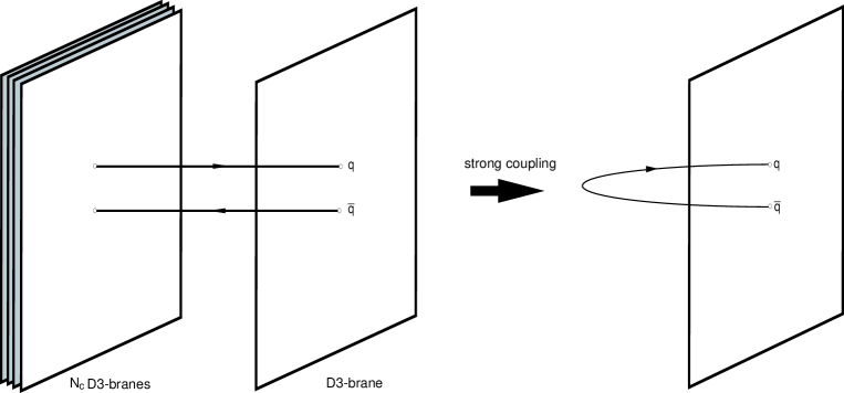
Figure 8: Wilson loop and confinement. We introduce the quark pair in terms of the W bosons associated to the symmetry breaking $U(N_{c}+1)\to U(N_{c})\times U(1)$, which we perform by separating a D3–brane. At strong coupling, as discussed earlier, the $N_{c}$ D3–branes are replaced by the background.

The quark anti-quark potential is read off from (19) and (181), after a suitable renormalization [131] –whose details we skip– of the otherwise divergent Nambu–Goto action. It is given by

$$E=f(0)L+2\int_{0}^{r_{f}}\frac{g(r)}{f(r)}\;\bigg{(}\sqrt{f^{2}(r)-f^{2}(0)}-f(r)\bigg{)}\;dr~{},$$ (188)

In this way, we can determine whether a supersymmetric gauge theory is confining or not from its gravity dual. It is possible to extract from the above formulas a sufficient condition for confinement [131]: If $f(r)$ is analytic, $f^{\prime}(r)$ is positive and $g(r)$ is smooth for $r\in(0,\infty)$, and if the integral of $g(r)/f^{2}(r)$ does not diverge, then there is confinement if either $f(0)\neq 0$ or $g(\tilde{r})\to\infty$ for some $r=\tilde{r}$, with $f(\tilde{r})\neq 0$. It is not hard to check that the first condition is accomplished in the MN solution. Notice that confinement reduces to the behaviour of the gravity dual at small radius which, from the point of view of the gauge theory, is the IR. The tension of the QCD string in the MN set up is finite (actually, proportional to $f(0)$): the theory confines.

5.8 Instantons

As discussed earlier, instantons in $\mathcal{N}=1$ SYM theory are responsible for breaking $U(1)_{R}$ to $\mathbb{Z}_{2N_{c}}$. The action of an instanton, from the field theory point of view, is given by

$$S_{\rm inst}=\frac{8\pi^{2}}{g_{YM}^{2}}+i\theta_{YM}~{}.$$ (189)

In the large $N_{c}$ limit, this breaking pattern is not apparent in the isometries of the MN background. Instantons can be identified with Euclidean D1–branes wrapping an $S^{2}$ which is orthogonal to the gauge theory directions [106]. The precise supersymmetric 2-cycle is defined by the equations

$$\theta=\tilde{\theta}~{},\quad\quad\quad\tilde{\varphi}=2\pi-\varphi~{},\quad\quad\quad\psi=(2n+1)\pi~{}.$$ (190)

In the UV we have to use the S-dual background, that is, the D1–brane should be replaced by a fundamental string (the instantons in the gauge theory being related to worldsheet instantons). As the MN configuration asymptotes to the so-called Abelian MN solution in the UV, we should use the latter to compute instanton effects. The upshot being that the Nambu–Goto action (plus the Wess–Zumino contribution),

$$S_{\rm NG}=\frac{1}{2\pi\alpha^{\prime}g_{s}}\int_{\cal W}d^{2}\xi~{}e^{-\phi}~{}\sqrt{e^{2h}+\frac{1}{4}(a-1)^{2}}-i\int_{\cal W}~{}B_{2}~{},$$ (191)

must be identified with the action of an instanton, $S_{\rm NG}=S_{\rm inst}$. When computing explicitly, we get

$$\frac{8\pi^{2}}{g_{YM}^{2}} = \frac{1}{2\pi\alpha^{\prime}g_{s}}\int_{\cal W}d^{2}\xi~{}e^{-\phi}~{}\sqrt{e^{2h}+\frac{1}{4}(a-1)^{2}}\,,$$ (192)

$$\theta_{YM} = 4N_{c}\psi_{0}~{}.$$ (194)

The latter expression tells us that only $\mathbb{Z}_{2N_{c}}$ rotations of the phase $\psi\to\psi+\frac{2\pi k}{N_{c}}$ leave the path integral invariant.

5.9 Finite Temperature Effects

We would like to shortly mention an interesting application of the gauge/gravity duality to confining theories at finite temperature. There is a conjectured deconfining phase transition in these theories, at a given temperature $T_{c}$, where a new state of matter appears; namely, the quark–gluon plasma. In recent years, the traditional view on quark–gluon plasma properties has changed. Instead of being thought of as a weakly interacting gas of quasiparticles, it is now viewed as a strongly coupled nearly perfect fluid [129]. As such, it is better described in terms of hydrodynamics. It is then a vital issue to characterize its transport properties such as the shear and bulk viscosities, $\eta$ and $\zeta$, the thermal and electric conductivity $\kappa_{T}$ and $\sigma$, the charge diffusion constant $D_{Q}$, the speed of sound $v_{s}$ and the entropy density $s$. Transport coefficients are hard to compute from first principles, even in perturbation theory, and are not amenable to lattice gauge theory techniques either (see, however, [122]). The uses of the gauge/gravity correspondence in this respect are of sound relevance.

The shear viscosity represents the transferred momentum between different layers of a fluid. It is computed in the high energy regime of field theories as a correlation function of the stress-energy tensor by the so-called Kubo formula

$$\eta=\lim_{w\to 0}~{}\frac{1}{2w}\int dtd^{3}\vec{x}~{}e^{iwt}~{}<[T_{xy}(\vec{x},t),T_{xy}(\vec{0},0)]>=-\lim_{w\to 0}~{}\frac{{\rm Im}~{}G_{xy,xy}^{\rm R}(w,\vec{0})}{w}~{},$$ (195)

where $G_{xy,xy}^{\rm R}(w,\vec{0})$ is the retarded Green function. This has been studied in detail when $T>>T_{c}$ in perturbative field theory. How can this be computed on the gravity side?

The gravity duals of finite temperature gauge theories involve black holes in asymptotically AdS backgrounds [141]. Hawking’s temperature and Bekenstein’s entropy of the gravitational background are identified with those of the gauge theory in thermal equilibrium. Given that transport properties correspond to near-equilibrium processes, and taking into account that $g_{\mu\nu}$ couples to the energy–momentum tensor and we wish to compute correlators of the kind given in (195), they can be studied by considering (metric) perturbations of the appropriate thermal supergravity background [120]. We will not explain this technically involved approach here. Instead, we would like to comment on a misterious feature that, even having being developed some twenty years ago, makes more sense under the a posteriori light of AdS/CFT. This goes under the name of the membrane paradigm [73].

The black hole membrane paradigm can be simply recasted as stating that the event horizon can be thought of as a high temperature classically radiating surface (see [135] for details). Being out of equilibrium, it presents all kinds of characteristic features of a dissipative system. Consider, for example, the shear viscosity. Let us start from a generic black hole background of the form

$$ds^{2}=-g_{tt}(r)dt^{2}+g_{xx}(r)d\vec{x}^{2}+g_{rr}(r)dr^{2}+Z(r)\tilde{g}_{ij}(y)dy^{i}dy^{j}~{},$$ (196)

where $r_{0}$ stands for the position of the black hole horizon. Without entering into details that are well out of the scope of these lectures, we would like to comment on a striking result. It turns out that the shear viscosity per unit of specific entropy of this configuration that follows from the membrane paradigm, fully coincides with the expression obtained by computing the lowest quasinormal frequency in this background [93],

$$\frac{\eta}{s}=T\left.\sqrt{\frac{\det g}{g_{tt}g_{rr}}}\;\right|_{r=r_{0}}~{}\int_{r_{0}}^{\infty}dr~{}\frac{g_{tt}g_{rr}}{g_{xx}\sqrt{\det g}}~{}.$$ (197)

Something similar happens with other transport coefficients. Furthermore (and remarkably enough), the above formula gives a universal value for backgrounds corresponding to duals of a huge class of supersymmetric gauge theories of the black brane form (196) [34],

$$\frac{\eta}{s}=\frac{1}{4\pi}~{},$$ (198)

in the regime in which it is well described by its gravity dual, i.e., at strong ’t Hooft coupling. This universality is related to that of the low energy absortion cross section for gravitons [44, 58, 94]. Furthermore, and most important to us, this ubiquitous value has been explicitely derived by direct computation of Kubo’s formula within the AdS/CFT framework for a wide class of relevant supergravity backgrounds [32]. This is quite a small value. For example, the same quantity for water under normal pressure and temperature is about 400 times higher. In good accord with this prediction, measurements at the Relativistic Heavy Ion Collider (RHIC) also suggest a small value for this ratio [129].

Let us quickly check how this result emerges within the membrane paradigm in the case of a finite temperature version of the Maldacena–Núñez background. It is given by the following 10d metric in the Einstein frame [33],

$$ds^{2}=C^{2}(r)\bigg{[}-\Delta_{1}^{2}(r)\,dt^{2}+d\vec{x}_{2}^{2}+\alpha^{\prime}g_{s}N_{c}\,\bigg{(}\frac{dr^{2}}{r^{2}~{}\Delta_{2}(r)^{2}}+e^{2\hat{h}(r)}\,d\Omega^{2}_{2}+\frac{1}{4}\,d\tilde{\Omega}^{2}_{2}+\frac{1}{4}\,e_{\psi}^{2}\bigg{)}\bigg{]}~{},$$ (199)

where $e_{\psi}=d\psi+\cos\theta\,d\phi+\cos\tilde{\theta}\,d\tilde{\phi}$, and the set of functions $C(r)$, $\Delta_{1}(r)$, $\Delta_{2}(r)$ and $\hat{h}(r)$, which are defined in [33], satisfy the identity

$$\Delta_{1}^{\prime}(r)\Delta_{2}(r)=\frac{\mu}{4rC(r)^{8}e^{2\hat{h}(r)}}~{},$$ (200)

$\mu$ being the near extremal parameter. This solution has a regular horizon $r_{0}$. One can compute the temperature of the black hole to be

$$2\pi T=\left.\frac{\mu}{\sqrt{\alpha^{\prime}g_{s}N}}~{}\frac{1}{C^{2}(r)\hat{h}(r)}\right|_{r=r_{0}}~{}.$$ (201)

Inserting this expression in (197), and using (200), it is not hard to verify that the universal value $1/4\pi$ is attained [34].

Plugging in units into (198), it is amusing to check that neither the Newton constant $G$ nor the speed of light $c$ appear in this expression. This seems to imply that it is not of relativistic or gravitational origin. The constants entering (198) are Planck’s $\hbar$ and Boltzmann’s $k_{B}$. It actually looks more quantum mechanical. Like the saturation of the uncertainty principle. Indeed, it has been conjectured that this value is a lower bound for any system in Nature [93, 94].

5.10 Adding Flavors

In order to introduce matter in the fundamental representation of the gauge group, it is necessary to incorporate an open string sector in the dual supergravity background. To do so, it seems natural to consider the addition of D–brane probes at a characteristic distance. Let us call them flavor branes. This distance will give a lower bound for the energy of a string stretched between both branes which is to be related with the mass of the quarks. It is interesting to point out that this is also suggested by ’t Hooft’s large $N_{c}$ arguments, since flavor corresponds to the presence of boundaries in the worldsheet and these amount to D–branes. It was originally proposed in the $AdS_{5}\times S^{5}$ case that addition of flavor corresponds to spacetime filling D7–branes [86]. Open strings coming into the stack of D3–branes where the gauge theory is defined, represent quarks and the fluctuations of these D7–branes provide the meson spectrum [97].

The addition of matter multiplets in supersymmetric gauge theories does not reduce the amount of supersymmetry. Therefore, the flavor branes have to be introduced into the configuration in a symmetry preserving way. At the probe approximation, the supersymmetric embedding of a D–brane probe is obtained by imposing the kappa-symmetry condition:

$$\Gamma_{\kappa}\,\epsilon\,=\,\epsilon\,\,,$$ (202)

where $\epsilon$ is a Killing spinor of the background and $\Gamma_{\kappa}$ is a matrix that depends on the embedding. In the absence of worldvolume gauge fields living on the probe D–brane,

$$\Gamma_{\kappa}\,=\,\frac{1}{(p+1)!\sqrt{-g}}\,\epsilon^{\mu_{1}\cdots\mu_{p+1}}\,(\tau_{3})^{\frac{p-3}{2}}\,i\tau_{2}\,\otimes\,\gamma_{\mu_{1}\cdots\mu_{p+1}}\,\,,$$ (203)

where $g$ is the determinant of the induced metric $g_{\mu\nu}$ and $\gamma_{\mu_{1}\cdots\mu_{p+1}}$ denotes the antisymmetrized product of the induced Dirac matrices. In order that the probe approximation remains valid and backreaction of the flavor branes do not need to be considered, we shall assume that we are in the so-called quenched approximation, $N_{f}<<N_{c}$. In the case of MN, flavor is introduced through D5–branes wrapping a two-cycle different from the one wrapped by the bunch of $N_{c}$ D5–branes defining the gauge theory [113]. There are no solutions at a fixed distance. This is related to the lack of moduli space in $\mathcal{N}=1$ theory. Other aspects that can be studied within this framework include $U(1)_{R}$ symmetry breaking by the formation of a squark condensate, non-smoothness of the massless quark limit, and $U(1)_{B}$ baryonic symmetry preservation. We have unfortunately no time to discuss these in the present lectures. Further work on the gauge/gravity duality in presence of flavors include [10]. Aspects of the meson spectrum were considered in [59], while meson decay at strong coupling has been recently discussed in [115, 41].

Many additional aspects of the gauge/gravity duality in confining theories would have deserved to be discussed in these lectures. For example, the mass spectrum of glueballs. These are composite objects whose constituents are nothing but gluons. The mass spectrum of these states is quite amenable to lattice studies [133]. By these means, it has been shown that they have a bound state spectrum, the lightest glueball being a scalar with a mass of 1630 MeV. The examination of this problem in the dual gravity background demands the study of fluctuations of supergravity fields. The linearized system is reduced to a Schrödinger problem whose eigenvalues are nothing but the desired spectrum. Remind that we have seen in the second lecture that fluctuations of the fields in the gravity side correspond to operators in the dual gauge theory. Thus, what this approach computes is a correlation function from which we can actually read the masses of the glueballs. In the MN setup, this issue has been addressed quite recently in [35, 17].

Appendix A Useful formulas

A.1 Conifold

The metric of the conifold and its resolved and deformed cousins are better described in terms of the following vielbein:

$$g^{1} = \frac{1}{\sqrt{2}}\left[-\sin\theta_{1}\,d\phi_{1}-\cos\psi\,\sin\theta_{2}\,d\phi_{2}+\sin\psi\,d\theta_{2}\right]$$ (204)

$$g^{2} = \frac{1}{\sqrt{2}}\left[d\theta_{1}-\sin\psi\,\sin\theta_{2}\,d\phi_{2}-\cos\psi\,d\theta_{2}\right]$$ (205)

$$g^{3} = \frac{1}{\sqrt{2}}\left[-\sin\theta_{1}\,d\phi_{1}+\cos\psi\,\sin\theta_{2}\,d\phi_{2}-\sin\psi\,d\theta_{2}\right]$$ (206)

$$g^{4} = \frac{1}{\sqrt{2}}\left[d\theta_{1}+\sin\psi\,\sin\theta_{2}\,d\phi_{2}+\cos\psi\,d\theta_{2}\right]$$ (207)

$$g^{5} = d\psi+\cos\theta_{1}\,d\phi_{1}+\cos\theta_{2}\,d\phi_{2}$$ (208)

The metric of $T^{1,1}$, for example, is then written as

$$ds^{2}(T^{1,1})=\frac{1}{6}\sum_{i=1}^{4}(g^{i})^{2}+\frac{1}{9}(g^{5})^{2}$$ (209)

Check, as a useful exercise, the following identities:

$$d(g^{1}\wedge g^{2}+g^{3}\wedge g^{4})=g^{5}\wedge(g^{1}\wedge g^{2}-g^{3}\wedge g^{4})$$ (210)

$$d(g^{1}\wedge g^{2}-g^{3}\wedge g^{4})=-g^{5}\wedge(g^{1}\wedge g^{3}+g^{2}\wedge g^{4})$$ (211)

Remind that $T^{1,1}$ is a $U(1)$ fibration over a Kähler–Einstein manifold, $S^{2}\times S^{2}$. The symplectic form of the 4d base manifold reads

$$J_{4}=\frac{1}{6}\,\bigg{(}\sin\theta_{1}\,d\theta_{1}\wedge d\phi_{1}+\sin\theta_{2}\,d\theta_{2}\wedge d\phi_{2}\bigg{)}~{}.$$ (212)

Given the conical structure of the variety, we can write the symplectic form of the conifold $J$ by means of $J_{4}$ and $g^{5}$

$$J=r^{2}\,J_{4}+\frac{r}{3}\,dr{\wedge}g^{5}~{}.$$ (213)

The reader should check that $dJ=0$. We can also define the $2$-form

$$w_{2}=\frac{1}{2}\bigg{(}g^{1}{\wedge}g^{2}+g^{3}{\wedge}g^{4}\bigg{)}=\frac{1}{2}\bigg{(}\sin\theta_{1}d\theta_{1}{\wedge}d\phi_{1}-\sin\theta_{2}d\theta_{2}{\wedge}d\phi_{2}\bigg{)}~{},$$ (214)

and the $3$-form $w_{3}$

$$w_{3}=g^{5}{\wedge}w_{2}~{}.$$ (215)

Both are closed

$$dw_{2}=dw_{3}=0~{}.$$ (216)

Furthermore, notice that

$$w_{2}{\wedge}w_{3} = \frac{1}{2}\bigg{(}g^{1}{\wedge}g^{2}+g^{3}{\wedge}g^{4}\bigg{)}{\wedge}g^{5}{\wedge}\frac{1}{2}\bigg{(}g^{1}{\wedge}g^{2}+g^{3}{\wedge}g^{4}\bigg{)}$$ (217)

$$= \frac{1}{2}g^{1}{\wedge}g^{2}{\wedge}g^{3}{\wedge}g^{4}{\wedge}g^{5}=54\,d{\rm Vol}(T^{1,1})~{}.$$ (218)

The following results are also useful throughout the text (in section 4):

$$w_{2}^{2} \equiv w_{2,ab}w_{2}^{ab}=g^{ac}g^{bd}w_{2,ab}w_{2,cd}=\frac{36}{r^{4}h}~{},$$ (219)

$$w_{3}^{2} \equiv w_{3,abc}w_{3}^{abc}=\frac{3^{5}4}{r^{6}h^{3/2}}~{},$$ (220)

$h=h(r)$ being the function appearing as a warp factor in the metric (122). Using the metric (111), it is straightforward to compute the volume of the base

$${\rm Vol}(T^{1,1})=\frac{16}{27}\pi^{3}~{}.$$ (221)

Thus,

$$L^{4}=\frac{27\pi}{4}g_{s}N(\alpha^{\prime})^{2}~{}.$$ (222)

A.2 Left invariant one forms

Let $L$ be an element of $SU(2)$. The left invariant one forms $w^{k}$, $k=1,2,3$, are defined by the expression

$$L^{\dagger}dL=\frac{i}{2}w^{k}\sigma_{k}~{},$$ (223)

where $\sigma_{k}$ are the Pauli matrices. The canonical basis is

$$w^{1} = \cos\phi d\theta+\sin\theta\sin\phi d\psi~{},$$ (224)

$$w^{2} = \sin\phi d\theta-\sin\theta\cos\phi d\psi~{},$$ (225)

$$w^{3} = d\phi+\cos\theta d\psi~{}.$$ (226)

Exercise: Check that parametrization of $L$ in terms of Euler angles,

$$L=e^{\frac{i}{2}\phi\sigma_{3}}e^{\frac{i}{2}\theta\sigma_{1}}e^{\frac{i}{2}\psi\sigma_{3}}~{},~{}~{}~{}~{}~{}~{}~{}0\leq\phi,\psi\leq 2\pi~{},~{}~{}~{}0\leq\theta\leq\pi~{},$$

leads to the canonical basis. It is useful to notice that $w^{k}=-i\rm Tr(\sigma_{k}L^{\dagger}dL)$.

A.3 Useful type IIB formulas

Let us recall the Lagrangian and equations of motion of type IIB supergravity. In the string frame, the action reads [126]:

$$S_{IIB} = \frac{1}{2\kappa^{2}}\int e^{-2\Phi}\left(d^{10}x\sqrt{-g}\,R+4~{}d\Phi\wedge\star d\Phi-\frac{1}{12}H_{[3]}\wedge\star H_{[3]}\right)$$ (227)

$$- \frac{1}{4\kappa^{2}}\int\bigg{(}F_{[1]}\wedge\star F_{[1]}+\frac{1}{6}F_{[3]}\wedge\star F_{[3]}+\frac{1}{240}F_{[5]}\wedge\star F_{[5]}-C_{[4]}\wedge F_{[3]}\wedge H_{[3]}\bigg{)}~{},$$ (228)

where

$$F_{[1]} = dC_{[0]}~{},$$

$$F_{[3]} = dC_{[2]}-C_{[0]}\,H_{[3]}~{},$$

$$H_{[3]} = dB_{[2]}~{},$$

$$F_{[5]} = dC_{[4]}-\frac{1}{2}\,C_{[2]}\wedge H_{[3]}+\frac{1}{2}\,B_{[2]}\wedge F_{[3]}~{},$$ (229)

supplemented by the additional on-shell constraint $F_{[5]}=\star F_{[5]}$. Let us recall the change to the Einstein frame by keeping careful track of the $g_{s}$ factors (following, for example, Ref.[77]). We start from

$$(g_{\mu\nu})_{\rm string}=g_{s}^{-1/2}\,e^{\Phi/2}\,(g_{\mu\nu})_{\rm Einstein}~{},$$ (230)

where $g_{s}=e^{\Phi(r\to\infty)}$ is the string coupling constant. Then,

$$\sqrt{|g|}_{\rm string}=(g_{s}^{-1/2}\,e^{\Phi/2})^{5}\,\sqrt{|g|}_{\rm Einstein}=g_{s}^{-5/2}\,e^{5\Phi/2}\,\sqrt{|g|}_{\rm Einstein}~{}.$$ (231)

In general, for any $p$–form

$$(F_{[p]}{\wedge}\star F_{[p]})_{\rm string}=g_{s}^{p/2}\,e^{-p\Phi/2}\,(F_{[p]}{\wedge}\star F_{[p]})_{\rm Einstein}~{}.$$ (232)

Reabsorbing the factor $g_{s}^{2}$ into the constant $\kappa^{2}$ by defining $\bar{\kappa}^{2}=g_{s}^{2}\kappa^{2}$, we can write the action in the Einstein frame as

$$S_{IIB} = \frac{1}{2\bar{\kappa}^{2}}\int\,\left(d^{10}x\sqrt{-g}R-\frac{1}{2}~{}d\Phi\wedge\star d\Phi-\frac{g_{s}}{12}\,e^{-\Phi}H_{[3]}\wedge\star H_{[3]}\right.$$

$$- \frac{1}{2}\,\bigg{[}e^{2\Phi}F_{[1]}\wedge\star F_{[1]}+\frac{g_{s}}{6}\,e^{\Phi}F_{[3]}\wedge\star F_{[3]}+\frac{g_{s}^{2}}{240}\,F_{[5]}\wedge\star F_{[5]}-\,g_{s}^{2}\,C_{[4]}\wedge F_{[3]}\wedge H_{[3]}\bigg{]}\bigg{)}~{},$$

where all quantities are given in the Einstein frame. Beside the Einstein equation,

$$R_{MN} = \frac{1}{2}\partial_{M}\phi\partial_{N}\phi+\frac{1}{2}e^{2\Phi}\partial_{M}C_{[0]}\partial_{N}C_{[0]}+\frac{g_{s}}{4}\,e^{-\Phi}\bigg{(}{H_{[3]}}_{MPQ}{H_{[3]}}_{N}^{~{}PQ}-\frac{1}{12}g_{MN}\,{H_{[3]}}^{2}\bigg{)}$$ (235)

$$+\frac{g_{s}^{2}}{96}{F_{[5]}}_{MPQRS}{F_{[5]}}_{N}^{~{}PQRS}+\frac{g_{s}}{4}\,e^{\Phi}\bigg{(}{F_{[3]}}_{MPQ}{F_{[3]}}_{N}^{~{}PQ}-\frac{1}{12}g_{MN}{F_{[3]}}^{2}\bigg{)}~{},$$

where we used $F_{[5]}^{2}=0$, the equations of motion include

$$\nabla^{2}\phi=F_{[1]}^{2}-\frac{g_{s}}{12}\,e^{-\Phi}\,H_{[3]}^{2}+\frac{g_{s}}{12}\,e^{\Phi}\,F_{[3]}^{2}~{},$$ (236)

$$d(e^{2\Phi}\star F_{[1]})=-g_{s}\,e^{\Phi}\,H_{[3]}\wedge\star F_{[3]}~{},$$ (237)

$$d(e^{\Phi}\star F_{[3]})=g_{s}\,F_{[5]}\wedge H_{[3]}~{},$$ (238)

$$d(e^{-\Phi}\star H_{[3]}-C_{[0]}\,e^{\Phi}\star F_{[3]})=-g_{s}\,F_{[5]}\wedge\left(F_{[3]}+C_{[0]}\,H_{[3]}\right)~{},$$ (239)

$$d(\star F_{[5]})=-F_{[3]}\wedge H_{[3]}~{},$$ (240)

and the Bianchi identities

$$dF_{[1]}=dH_{[3]}=0~{},\qquad dF_{[3]}=-F_{[1]}\wedge H_{[3]}~{},\qquad dF_{[5]}=-F_{[3]}\wedge H_{[3]}~{}.$$ (241)

References

- [1] B. S. Acharya, “On realising N = 1 super Yang-Mills in M theory,” arXiv:hep-th/0011089.
- [2] B. S. Acharya, “Confining strings from G(2)-holonomy spacetimes,” arXiv:hep-th/0101206.
- [3] B. S. Acharya and S. Gukov, “M theory and Singularities of Exceptional Holonomy Manifolds,” Phys. Rept. 392, 121 (2004) [arXiv:hep-th/0409191].
- [4] B. S. Acharya and C. Vafa, “On domain walls of N = 1 supersymmetric Yang-Mills in four dimensions,” arXiv:hep-th/0103011.
- [5] B. Acharya and E. Witten, “Chiral fermions from manifolds of G(2) holonomy,” arXiv:hep-th/0109152.
- [6] I. Affleck, M. Dine and N. Seiberg, “Dynamical Supersymmetry Breaking In Supersymmetric QCD,” Nucl. Phys. B 241, 493 (1984).
- [7] O. Aharony, “The non-AdS/non-CFT correspondence, or three different paths to QCD,” arXiv:hep-th/0212193.
- [8] O. Aharony, S. S. Gubser, J. M. Maldacena, H. Ooguri and Y. Oz, “Large N field theories, string theory and gravity,” Phys. Rept. 323, 183 (2000) [arXiv:hep-th/9905111].
- [9] R. Apreda, F. Bigazzi, A. L. Cotrone, M. Petrini and A. Zaffaroni, “Some comments on N = 1 gauge theories from wrapped branes,” Phys. Lett. B 536, 161 (2002) [arXiv:hep-th/0112236].
- [10] R. Apreda, J. Erdmenger, N. Evans, J. Grosse and Z. Guralnik, “Instantons on D7 brane probes and AdS/CFT with flavour,” arXiv:hep-th/0601130.
- [11] M. Atiyah, J. M. Maldacena and C. Vafa, “An M-theory flop as a large N duality,” J. Math. Phys. 42, 3209 (2001) [arXiv:hep-th/0011256].
- [12] M. Atiyah and E. Witten, “M-theory dynamics on a manifold of G(2) holonomy,” Adv. Theor. Math. Phys. 6, 1 (2003) [arXiv:hep-th/0107177].
- [13] J. Babington, J. Erdmenger, N. J. Evans, Z. Guralnik and I. Kirsch, “Chiral symmetry breaking and pions in non-supersymmetric gauge/gravity duals,” Phys. Rev. D 69, 066007 (2004) [arXiv:hep-th/0306018]; “A gravity dual of chiral symmetry breaking,” Fortsch. Phys. 52, 578 (2004) [arXiv:hep-th/0312263].
- [14] D. Bak, M. Gutperle and S. Hirano, “A dilatonic deformation of AdS(5) and its field theory dual,” JHEP 0305, 072 (2003) [arXiv:hep-th/0304129].
- [15] J. D. Bekenstein, “Black Holes And Entropy,” Phys. Rev. D 7, 2333 (1973). “Generalized Second Law Of Thermodynamics In Black Hole Physics,” Phys. Rev. D 9, 3292 (1974).
- [16] D. Berenstein, J. M. Maldacena and H. Nastase, “Strings in flat space and pp waves from N = 4 super Yang Mills,” JHEP 0204, 013 (2002) [arXiv:hep-th/0202021].
- [17] M. Berg, M. Haack and W. Muck, “Bulk dynamics in confining gauge theories,” Nucl. Phys. B 736, 82 (2006) [arXiv:hep-th/0507285].
- [18] M. Bershadsky, S. Cecotti, H. Ooguri and C. Vafa, “Kodaira-Spencer theory of gravity and exact results for quantum string amplitudes,” Commun. Math. Phys. 165, 311 (1994) [arXiv:hep-th/9309140].
- [19] M. Bershadsky, C. Vafa and V. Sadov, “D-Branes and Topological Field Theories,” Nucl. Phys. B 463, 420 (1996) [arXiv:hep-th/9511222].
- [20] M. Bertolini, “Four lectures on the gauge-gravity correspondence,” Int. J. Mod. Phys. A 18, 5647 (2003) [arXiv:hep-th/0303160].
- [21] M. Bertolini, P. Di Vecchia, M. Frau, A. Lerda and R. Marotta, “N = 2 gauge theories on systems of fractional D3/D7 branes,” Nucl. Phys. B 621, 157 (2002) [arXiv:hep-th/0107057].
- [22] M. Bertolini, P. Di Vecchia, M. Frau, A. Lerda and R. Marotta, “More anomalies from fractional branes,” Phys. Lett. B 540, 104 (2002) [arXiv:hep-th/0202195].
- [23] M. Bertolini and P. Merlatti, “A note on the dual of N = 1 super Yang-Mills theory,” Phys. Lett. B 556, 80 (2003) [arXiv:hep-th/0211142].
- [24] F. Bigazzi, A. L. Cotrone and A. Zaffaroni, “N = 2 gauge theories from wrapped five-branes,” Phys. Lett. B 519, 269 (2001) [arXiv:hep-th/0106160].
- [25] F. Bigazzi, A. L. Cotrone, M. Petrini and A. Zaffaroni, “Supergravity duals of supersymmetric four dimensional gauge theories,” Riv. Nuovo Cim. 25N12, 1 (2002) [arXiv:hep-th/0303191].
- [26] M. Blau, J. Figueroa-O’Farrill, C. Hull and G. Papadopoulos, “Penrose limits and maximal supersymmetry,” Class. Quant. Grav. 19, L87 (2002) [arXiv:hep-th/0201081].
- [27] N. P. Bobev, H. Dimov and R. C. Rashkov, “Semiclassical strings, dipole deformations of N = 1 SYM and decoupling of KK modes,” arXiv:hep-th/0511216.
- [28] J. de Boer, H. Ooguri, H. Robins and J. Tannenhauser, “String theory on AdS(3),” JHEP 9812, 026 (1998) [arXiv:hep-th/9812046].
- [29] H. J. Boonstra, K. Skenderis and P. K. Townsend, “The domain wall/QFT correspondence,” JHEP 9901, 003 (1999) [arXiv:hep-th/9807137].
- [30] A. Brandhuber, J. Gomis, S. S. Gubser and S. Gukov, “Gauge theory at large N and new G(2) holonomy metrics,” Nucl. Phys. B 611, 179 (2001) [arXiv:hep-th/0106034].
- [31] R. Bryant and S. Salamon, “On The Construction Of Some Complete Metrices With Expectional Holonomy,” Duke Math. J. 58, 829 (1989).
- [32] A. Buchel, “On universality of stress-energy tensor correlation functions in supergravity,” Phys. Lett. B 609, 392 (2005) [arXiv:hep-th/0408095].
- [33] A. Buchel and A. R. Frey, “Comments on supergravity dual of pure N = 1 super Yang Mills theory with unbroken chiral symmetry,” Phys. Rev. D 64, 064007 (2001) [arXiv:hep-th/0103022].
- [34] A. Buchel and J. T. Liu, “Universality of the shear viscosity in supergravity,” Phys. Rev. Lett. 93, 090602 (2004) [arXiv:hep-th/0311175].
- [35] E. Caceres and C. Nunez, “Glueballs of super Yang-Mills from wrapped branes,” JHEP 0509, 027 (2005) [arXiv:hep-th/0506051].
- [36] F. Cachazo, K. A. Intriligator and C. Vafa, “A large N duality via a geometric transition,” Nucl. Phys. B 603, 3 (2001) [arXiv:hep-th/0103067].
- [37] P. Candelas and X. C. de la Ossa, “Comments On Conifolds,” Nucl. Phys. B 342, 246 (1990).
- [38] R. Casero, C. Nunez and A. Paredes, “Towards the string dual of N = 1 SQCD-like theories,” arXiv:hep-th/0602027.
- [39] A. H. Chamseddine and M. S. Volkov, “Non-Abelian BPS monopoles in N = 4 gauged supergravity,” Phys. Rev. Lett. 79, 3343 (1997) [arXiv:hep-th/9707176].
- [40] S. R. Coleman and E. Weinberg, “Radiative Corrections As The Origin Of Spontaneous Symmetry Breaking,” Phys. Rev. D 7, 1888 (1973).
- [41] A. L. Cotrone, L. Martucci and W. Troost, “String splitting and strong coupling meson decay,” arXiv:hep-th/0511045.
- [42] E. Cremmer, B. Julia and J. Scherk, “Supergravity Theory In 11 Dimensions,” Phys. Lett. B 76, 409 (1978).
- [43] J. Dai, R. G. Leigh and J. Polchinski, “New Connections Between String Theories,” Mod. Phys. Lett. A 4, 2073 (1989).
- [44] S. R. Das, G. W. Gibbons and S. D. Mathur, “Universality of low energy absorption cross sections for black holes,” Phys. Rev. Lett. 78, 417 (1997) [arXiv:hep-th/9609052].
- [45] R. Dijkgraaf and C. Vafa, “Matrix models, topological strings, and supersymmetric gauge theories,” Nucl. Phys. B 644, 3 (2002) [arXiv:hep-th/0206255].
- [46] See, for example, J. Distler and C. Vafa, “A Critical Matrix Model At C = 1,” Mod. Phys. Lett. A 6, 259 (1991). M. Kontsevich, “Intersection theory on the moduli space of curves and the matrix Airy function,” Commun. Math. Phys. 147, 1 (1992).
- [47] P. Di Vecchia, “N = 1 super Yang-Mills from D branes,” arXiv:hep-th/0403216.
- [48] P. Di Vecchia, A. Lerda and P. Merlatti, “N = 1 and N = 2 super Yang-Mills theories from wrapped branes,” Nucl. Phys. B 646, 43 (2002) [arXiv:hep-th/0205204].
- [49] M. R. Douglas and S. H. Shenker, “Dynamics of SU(N) supersymmetric gauge theory,” Nucl. Phys. B 447, 271 (1995) [arXiv:hep-th/9503163].
- [50] G. R. Dvali and M. A. Shifman, “Domain walls in strongly coupled theories,” Phys. Lett. B 396, 64 (1997) [Erratum-ibid. B 407, 452 (1997)] [arXiv:hep-th/9612128].
- [51] J. D. Edelstein, W. G. Fuertes, J. Mas and J. M. Guilarte, “Phases of dual superconductivity and confinement in softly broken N = 2 supersymmetric Yang-Mills theories,” Phys. Rev. D 62, 065008 (2000) [arXiv:hep-th/0001184].
- [52] J. D. Edelstein, M. Marino and J. Mas, “Whitham hierarchies, instanton corrections and soft supersymmetry breaking in N = 2 SU(N) super Yang-Mills theory,” Nucl. Phys. B 541, 671 (1999) [arXiv:hep-th/9805172].
- [53] J. D. Edelstein and C. Núñez, “D6 branes and M-theory geometrical transitions from gauged supergravity,” JHEP 0104, 028 (2001) [arXiv:hep-th/0103167].
- [54] J. D. Edelstein, K. Oh and R. Tatar, “Orientifold, geometric transition and large N duality for SO/Sp gauge theories,” JHEP 0105, 009 (2001) [arXiv:hep-th/0104037].
- [55] J. D. Edelstein, A. Paredes and A. V. Ramallo, “Wrapped branes with fluxes in 8d gauged supergravity,” JHEP 0212, 075 (2002) [arXiv:hep-th/0207127].
- [56] J. D. Edelstein, A. Paredes and A. V. Ramallo, “Let’s twist again: General metrics of G(2) holonomy from gauged supergravity,” JHEP 0301, 011 (2003) [arXiv:hep-th/0211203].
- [57] J. D. Edelstein, A. Paredes and A. V. Ramallo, “Singularity resolution in gauged supergravity and conifold unification,” Phys. Lett. B 554, 197 (2003) [arXiv:hep-th/0212139].
- [58] R. Emparan, “Absorption of scalars by extended objects,” Nucl. Phys. B 516, 297 (1998) [arXiv:hep-th/9706204].
- [59] J. Erdmenger and I. Kirsch, “Mesons in gauge/gravity dual with large number of fundamental fields,” JHEP 0412, 025 (2004) [arXiv:hep-th/0408113].
- [60] D. Z. Freedman, C. Nunez, M. Schnabl and K. Skenderis, “Fake supergravity and domain wall stability,” Phys. Rev. D 69, 104027 (2004) [arXiv:hep-th/0312055].
- [61] J. P. Gauntlett, N. Kim, D. Martelli and D. Waldram, “Wrapped fivebranes and N = 2 super Yang-Mills theory,” Phys. Rev. D 64, 106008 (2001) [arXiv:hep-th/0106117].
- [62] J. P. Gauntlett, N. w. Kim, D. Martelli and D. Waldram, “Fivebranes wrapped on SLAG three-cycles and related geometry,” JHEP 0111, 018 (2001) [arXiv:hep-th/0110034].
- [63] G. W. Gibbons, D. N. Page and C. N. Pope, “Einstein Metrics On S**3 R**3 And R**4 Bundles,” Commun. Math. Phys. 127, 529 (1990).
- [64] R. Gopakumar and C. Vafa, “On the gauge theory/geometry correspondence,” Adv. Theor. Math. Phys. 3, 1415 (1999) [arXiv:hep-th/9811131].
- [65] A. Gorsky, A. Marshakov, A. Mironov and A. Morozov, “RG equations from Whitham hierarchy,” Nucl. Phys. B 527, 690 (1998) [arXiv:hep-th/9802007].
- [66] D. J. Gross and F. Wilczek, “Ultraviolet Behavior Of Non-Abelian Gauge Theories,” Phys. Rev. Lett. 30, 1343 (1973). H. D. Politzer, “Reliable Perturbative Results For Strong Interactions?,” Phys. Rev. Lett. 30, 1346 (1973).
- [67] S. S. Gubser, I. R. Klebanov and A. M. Polyakov, “Gauge theory correlators from non-critical string theory,” Phys. Lett. B 428, 105 (1998) [arXiv:hep-th/9802109].
- [68] S. S. Gubser, “Einstein manifolds and conformal field theories,” Phys. Rev. D 59, 025006 (1999) [arXiv:hep-th/9807164].
- [69] U. Gursoy, S. A. Hartnoll and R. Portugues, “The chiral anomaly from M theory,” Phys. Rev. D 69, 086003 (2004) [arXiv:hep-th/0311088].
- [70] U. Gursoy and C. Nunez, “Dipole deformations of N = 1 SYM and supergravity backgrounds with U(1) x U(1) global symmetry,” Nucl. Phys. B 725, 45 (2005) [arXiv:hep-th/0505100].
- [71] R. Haag, J. T. Lopuszanski and M. Sohnius, “All Possible Generators Of Supersymmetries Of The S Matrix,” Nucl. Phys. B 88, 257 (1975).
- [72] A. Hanany, M. J. Strassler and A. Zaffaroni, “Confinement and strings in MQCD,” Nucl. Phys. B 513, 87 (1998) [arXiv:hep-th/9707244].
- [73] R. S. Hanni and R. Ruffini, “Lines of force of a point charge near a Schwarzschild black hole,” Phys. Rev. D 8, 3259 (1973).
- [74] S. A. Hartnoll and R. Portugues, “Deforming baryons into confining strings,” Phys. Rev. D 70, 066007 (2004) [arXiv:hep-th/0405214].
- [75] S. W. Hawking, “Black Holes And Thermodynamics,” Phys. Rev. D 13, 191 (1976).
- [76] R. Hernandez and K. Sfetsos, “Branes with fluxes wrapped on spheres,” JHEP 0207, 045 (2002) [arXiv:hep-th/0205099].
- [77] C. P. Herzog and I. R. Klebanov, “Gravity duals of fractional branes in various dimensions,” Phys. Rev. D 63, 126005 (2001) [arXiv:hep-th/0101020].
- [78] C. P. Herzog and I. R. Klebanov, “On string tensions in supersymmetric SU(M) gauge theory,” Phys. Lett. B 526, 388 (2002) [arXiv:hep-th/0111078].
- [79] C. P. Herzog, I. R. Klebanov and P. Ouyang, “D-branes on the conifold and N = 1 gauge/gravity dualities,” arXiv:hep-th/0205100.
- [80] T. J. Hollowood, V. V. Khoze, W. J. Lee and M. P. Mattis, “Breakdown of cluster decomposition in instanton calculations of the gluino condensate,” Nucl. Phys. B 570, 241 (2000) [arXiv:hep-th/9904116].
- [81] G. ’t Hooft, “A Planar Diagram Theory For Strong Interactions,” Nucl. Phys. B 72, 461 (1974).
- [82] G. ’t Hooft, “Dimensional reduction in quantum gravity,” arXiv:gr-qc/9310026.
- [83] P. Horava, “Background Duality Of Open String Models,” Phys. Lett. B 231, 251 (1989).
- [84] E. Imeroni, “The gauge/string correspondence towards realistic gauge theories,” arXiv:hep-th/0312070.
- [85] N. Itzhaki, J. M. Maldacena, J. Sonnenschein and S. Yankielowicz, “Supergravity and the large N limit of theories with sixteen supercharges,” Phys. Rev. D 58, 046004 (1998) [arXiv:hep-th/9802042].
- [86] A. Karch and E. Katz, “Adding flavor to AdS/CFT,” JHEP 0206, 043 (2002) [arXiv:hep-th/0205236].
- [87] Y. Kinar, E. Schreiber and J. Sonnenschein, “Q anti-Q potential from strings in curved spacetime: Classical results,” Nucl. Phys. B 566, 103 (2000) [arXiv:hep-th/9811192].
- [88] I. R. Klebanov and N. A. Nekrasov, “Gravity duals of fractional branes and logarithmic RG flow,” Nucl. Phys. B 574, 263 (2000) [arXiv:hep-th/9911096].
- [89] I. R. Klebanov, P. Ouyang and E. Witten, “A gravity dual of the chiral anomaly,” Phys. Rev. D 65, 105007 (2002) [arXiv:hep-th/0202056].
- [90] I. R. Klebanov and M. J. Strassler, “Supergravity and a confining gauge theory: Duality cascades and SB-resolution of naked singularities,” JHEP 0008, 052 (2000) [arXiv:hep-th/0007191].
- [91] I. R. Klebanov and A. A. Tseytlin, “Gravity duals of supersymmetric SU(N) x SU(N+M) gauge theories,” Nucl. Phys. B 578, 123 (2000) [arXiv:hep-th/0002159].
- [92] I. R. Klebanov and E. Witten, “Superconformal field theory on threebranes at a Calabi-Yau singularity,” Nucl. Phys. B 536, 199 (1998) [arXiv:hep-th/9807080].
- [93] P. Kovtun, D. T. Son and A. O. Starinets, “Holography and hydrodynamics: Diffusion on stretched horizons,” JHEP 0310, 064 (2003) [arXiv:hep-th/0309213].
- [94] P. Kovtun, D. T. Son and A. O. Starinets, “Viscosity in strongly interacting quantum field theories from black hole physics,” Phys. Rev. Lett. 94, 111601 (2005) [arXiv:hep-th/0405231].
- [95] M. Krasnitz, “A two point function in a cascading N = 1 gauge theory from supergravity,” arXiv:hep-th/0011179.
- [96] M. Krasnitz, “Correlation functions in a cascading N = 1 gauge theory from supergravity,” JHEP 0212, 048 (2002) [arXiv:hep-th/0209163].
- [97] M. Kruczenski, D. Mateos, R. C. Myers and D. J. Winters, “Meson spectroscopy in AdS/CFT with flavour,” JHEP 0307, 049 (2003) [arXiv:hep-th/0304032].
- [98] J. M. F. Labastida and M. Marino, “Polynomial invariants for torus knots and topological strings,” Commun. Math. Phys. 217, 423 (2001) [arXiv:hep-th/0004196].
- [99] A. Loewy and J. Sonnenschein, “On the holographic duals of N = 1 gauge dynamics,” JHEP 0108, 007 (2001) [arXiv:hep-th/0103163].
- [100] O. Lunin and J. Maldacena, “Deforming field theories with U(1) x U(1) global symmetry and their gravity duals,” JHEP 0505, 033 (2005) [arXiv:hep-th/0502086].
- [101] K. Maeda, M. Natsuume and T. Okamura, “Viscosity of gauge theory plasma with a chemical potential from AdS/CFT,” arXiv:hep-th/0602010.
- [102] J. M. Maldacena, “The large N limit of superconformal field theories and supergravity,” Adv. Theor. Math. Phys. 2, 231 (1998) [Int. J. Theor. Phys. 38, 1113 (1999)] [arXiv:hep-th/9711200].
- [103] J. M. Maldacena, “Wilson loops in large N field theories,” Phys. Rev. Lett. 80, 4859 (1998) [arXiv:hep-th/9803002].
- [104] J. M. Maldacena and H. Nastase, “The supergravity dual of a theory with dynamical supersymmetry breaking,” JHEP 0109, 024 (2001) [arXiv:hep-th/0105049].
- [105] J. M. Maldacena and C. Núñez, “Supergravity description of field theories on curved manifolds and a no go theorem,” Int. J. Mod. Phys. A 16, 822 (2001) [arXiv:hep-th/0007018].
- [106] J. M. Maldacena and C. Núñez, “Towards the large N limit of pure N = 1 super Yang Mills,” Phys. Rev. Lett. 86, 588 (2001) [arXiv:hep-th/0008001].
- [107] M. Mariño, “The geometry of supersymmetric gauge theories in four dimensions,” arXiv:hep-th/9701128.
- [108] D. Martelli and J. Sparks, “Toric geometry, Sasaki-Einstein manifolds and a new infinite class of AdS/CFT duals,” arXiv:hep-th/0411238.
- [109] J. Mas, “Shear viscosity from R-charged AdS black holes,” arXiv:hep-th/0601144.
- [110] P. Merlatti, “N = 1 super Yang-Mills theories and wrapped branes,” Class. Quant. Grav. 20, S541 (2003) [arXiv:hep-th/0212203].
- [111] R. C. Myers, “Dielectric-branes,” JHEP 9912, 022 (1999) [arXiv:hep-th/9910053].
- [112] V. A. Novikov, M. A. Shifman, A. I. Vainshtein and V. I. Zakharov, “Exact Gell-Mann-Low Function Of Supersymmetric Yang-Mills Theories From Instanton Calculus,” Nucl. Phys. B 229, 381 (1983).
- [113] C. Nunez, A. Paredes and A. V. Ramallo, “Flavoring the gravity dual of N = 1 Yang-Mills with probes,” JHEP 0312, 024 (2003) [arXiv:hep-th/0311201].
- [114] H. Ooguri and C. Vafa, “Knot invariants and topological strings,” Nucl. Phys. B 577, 419 (2000) [arXiv:hep-th/9912123]. “Worldsheet derivation of a large N duality,” Nucl. Phys. B 641, 3 (2002) [arXiv:hep-th/0205297].
- [115] K. Peeters, J. Sonnenschein and M. Zamaklar, “Holographic decays of large-spin mesons,” arXiv:hep-th/0511044.
- [116] R. Penrose, “Any space-time has a plane wave as a limit.” Differential geometry and relativity, Reidel, Dordrecht, 1976, pp.271–275.
- [117] J. Polchinski, “Dirichlet-Branes and Ramond-Ramond Charges,” Phys. Rev. Lett. 75, 4724 (1995) [arXiv:hep-th/9510017].
- [118] J. Polchinski and M. J. Strassler, “The string dual of a confining four-dimensional gauge theory,” arXiv:hep-th/0003136.
- [119] J. Polchinski and L. Susskind, “String theory and the size of hadrons,” arXiv:hep-th/0112204.
- [120] G. Policastro, D. T. Son and A. O. Starinets, “The shear viscosity of strongly coupled N = 4 supersymmetric Yang-Mills plasma,” Phys. Rev. Lett. 87, 081601 (2001) [arXiv:hep-th/0104066].
- [121] S. J. Rey and J. T. Yee, “Macroscopic strings as heavy quarks in large N gauge theory and anti-de Sitter supergravity,” Eur. Phys. J. C 22, 379 (2001) [arXiv:hep-th/9803001].
- [122] S. Sakai and A. Nakamura, “Transport coefficient of gluon plasma from lattice QCD,” PoS LAT2005, 186 (2005) [arXiv:hep-lat/0510100].
- [123] A. Salam and E. Sezgin, “D = 8 Supergravity,” Nucl. Phys. B 258, 284 (1985).
- [124] O. Saremi, “The viscosity bound conjecture and hydrodynamics of M2-brane theory at finite chemical potential,” arXiv:hep-th/0601159.
- [125] M. Schvellinger and T. A. Tran, “Supergravity duals of gauge field theories from SU(2) x U(1) gauged supergravity in five dimensions,” JHEP 0106, 025 (2001) [arXiv:hep-th/0105019].
- [126] J. H. Schwarz, “Covariant Field Equations Of Chiral N=2 D = 10 Supergravity,” Nucl. Phys. B226, 269 (1983).
- [127] N. Seiberg, “The Power of holomorphy: Exact results in 4-D SUSY field theories,” arXiv:hep-th/9408013.
- [128] N. Seiberg and E. Witten, “Electric - magnetic duality, monopole condensation, and confinement in N=2 supersymmetric Yang-Mills theory,” Nucl. Phys. B 426, 19 (1994) [Erratum-ibid. B 430, 485 (1994)] [arXiv:hep-th/9407087].
- [129] E. Shuryak, “Why does the quark gluon plasma at RHIC behave as a nearly ideal fluid?,” Prog. Part. Nucl. Phys. 53, 273 (2004) [arXiv:hep-ph/0312227].
- [130] D. T. Son and A. O. Starinets, “Hydrodynamics of R-charged black holes,” arXiv:hep-th/0601157.
- [131] J. Sonnenschein, “What does the string / gauge correspondence teach us about Wilson loops?,” arXiv:hep-th/0003032.
- [132] M. J. Strassler, “The duality cascade,” arXiv:hep-th/0505153.
- [133] M. J. Teper, “Glueball masses and other physical properties of SU(N) gauge theories in D = 3+1: A review of lattice results for theorists,” arXiv:hep-th/9812187.
- [134] M. Teper, “Large-N gauge theories: Lattice perspectives and conjectures,” arXiv:hep-th/0412005.
- [135] K. S. Thorne, R. H. Price and D. A. Macdonald (eds.), “Black Holes: The Membrane Paradigm,” Yale University Press, New Haven (1986).
- [136] C. Vafa, “Superstrings and topological strings at large N,” J. Math. Phys. 42, 2798 (2001) [arXiv:hep-th/0008142].
- [137] M. Vonk, “A mini-course on topological strings,” arXiv:hep-th/0504147.
- [138] E. Witten, “Topological Quantum Field Theory,” Commun. Math. Phys. 117, 353 (1988).
- [139] E. Witten, “Branes and the dynamics of QCD,” Nucl. Phys. B 507, 658 (1997) [arXiv:hep-th/9706109].
- [140] E. Witten, “Anti-de Sitter space and holography,” Adv. Theor. Math. Phys. 2, 253 (1998) [arXiv:hep-th/9802150].
- [141] E. Witten, “Anti-de Sitter space, thermal phase transition, and confinement in gauge theories,” Adv. Theor. Math. Phys. 2, 505 (1998) [arXiv:hep-th/9803131].