The Non-BPS Black Hole Attractor Equation

Abstract:

We study the attractor mechanism for extremal non-BPS black holes with an infinite throat near horizon geometry, developing, as we do so, a physical argument as to why such a mechanism does not exist in non-extremal cases. We present a detailed derivation of the non-supersymmetric attractor equation. This equation defines the stabilization of moduli near the black hole horizon: the fixed moduli take values specified by electric and magnetic charges corresponding to the fluxes in a Calabi Yau compactification of string theory. They also define the so-called double-extremal solutions. In some examples, studied previously by Tripathy and Trivedi, we solve the equation and show that the moduli are fixed at values which may also be derived from the critical points of the black hole potential.

1 Introduction

The supersymmetric black hole attractor mechanism was introduced in [1]-[3] and studied in the context of string theory in [4] and [5]. The possibility of non-supersymmetric black holes attractors was initially introduced in [6], where the concept of the effective “black hole potential” was proposed. In general such a potential is a function of electric and magnetic charges and scalar-dependent vector couplings. For ${\cal N}=2$ supergravity $V_{BH}=|{\cal D}Z|^{2}+|Z|^{2}$, where $Z$ is the black hole central charge, the charge of the graviphoton.

The attractor mechanism for non-supersymmetric black holes was recently studied in [7] and [8]; examples were given and some important special features were described. In supersymmetric black hole attractors the moduli near the black hole horizon are always attracted to their fixed values since the attractor point is the minimum of the potential ([6]). For non-supersymmetric black holes the critical point of the black hole potential may not be a minimum — it was stressed in [7] and [8] that only the critical points of the potential which are a minima of the black hole potentials are the true attractor points.

In this paper we shall explore various aspects of non-BPS attractors. We commence, in Section 2, by analyzing the differences between extremal (zero temperature) and non-extremal black holes. By developing an analysis of the scalar field dynamics in both situations, we are able to construct a physical argument as to why one would expect only extremal black holes to attract. The essential geometric difference between the two cases is that extremal black holes possess an infinite throat where the physical distance to the horizon is infinite; this is in contrast to the non-extremal case, where this physical distance is finite. Since the distance acts as an evolution parameter for the scalar fields, it is only in the former case that the field can reach its attractor value, and forget its initial conditions.

In Section 3 we analyze the double-extremal black hole introduced in [9] and further developed in [10] and [11]. These solutions have everywhere-constant scalar fields, a simplification that allows us to study them in some detail.

It was shown in [12] that in effective ${\cal N}=2$ supergravity, instead of solving the equation for the extremum of the black hole potential, one can use the attractor equation in the form:

$$H_{3}=2{\rm Im}\left[\,Z\,\overline{\Omega}_{3}+\overline{\mathcal{D}}_{\bar{a}}\overline{Z}G^{\bar{a}a}{\mathcal{D}}_{a}{\Omega}_{3}\right]_{\partial V_{BH}=0}$$ (1)

The detailed form of the equation $\partial V_{BH}=0$ was presented in [6] and it requires that $2(\mathcal{D}_{a}Z)\bar{Z}+iC_{abc}G^{b\bar{b}}G^{c\bar{c}}\bar{\mathcal{D}}_{\bar{b}}\bar{Z}\bar{\mathcal{D}}_{\bar{c}}\bar{Z}=0$. This form can be used to make (1) explicit. This equation has been already tested in an example of a non-BPS black hole in [13]. In Section 4 we use this to establish a convenient and useful form of the non-BPS black hole attractor equation:

$$H_{3}=2\mbox{Im}\left[Z\,\overline{\Omega}_{3}-\frac{(\overline{\mathcal{D}}_{\bar{a}}\overline{\mathcal{D}}_{\bar{b}}\overline{Z})G^{\bar{a}a}G^{\bar{b}b}{\mathcal{D}}_{{b}}{Z}}{2{Z}}{{\mathcal{D}}}_{{a}}{\Omega}_{3}\right]\ .$$ (2)

In Section 5 we confirm the validity of the above by solving it directly for some of the examples from [8]. In these examples the attractor points were identified in [8] by solving the equation $\partial_{a}V_{BH}=0$. Here we will solve equation (2) and find both supersymmetric attractors with ${\mathcal{D}}_{{c}}{Z}=0$ and the non-supersymmetric ones with ${\mathcal{D}}_{{c}}{Z}\neq 0$. In the supersymmetric case the second term in (2) vanishes. However, in the non-supersymmetric case it conspires with the first term so that the moduli have to become function of charges to satisfy the equation. We also present an example of a double extremal non-BPS black hole.

Finally, we discuss the relation between non-BPS attractors and the O’Raifeartaigh model of spontaneous SUSY-breaking. In both cases the system cannot, by design, go to the supersymmetric minimum and therefore is stable.

2 Extremality and Attractiveness

Here we present the main features of the stabilization of moduli near a black hole horizon. We confirm, with a detailed explanation, that such stabilization is not necessarily related to unbroken supersymmetry and, in fact, that the existence of attractor-like behavior depends on the extremality (or otherwise) of the black hole.

We follow [6] and start by writing down the bosonic part of the Einstein-Maxwell action coupled to some Abelian vector fields:

$$-{R\over 2}+G_{a\bar{a}}\partial_{\mu}z^{a}\partial_{\nu}\bar{z}^{\bar{a}}g^{\mu\nu}+{\rm Im}{\cal N}_{\Lambda\Sigma}{\cal F}^{\Lambda}_{\mu\nu}{\cal F}^{\Sigma}_{\lambda\rho}g^{\mu\lambda}g^{\nu\rho}+{\rm Re}{\cal N}_{\Lambda\Sigma}{\cal F}^{\Lambda}_{\mu\nu}\left(\ast{\cal F}^{\Sigma}_{\lambda\rho}\right)g^{\mu\lambda}g^{\nu\rho}\ .$$ (3)

This action may have an arbitrary scalar metric $G_{a\bar{a}}$ and arbitrary scalar dependent vector couplings ${\rm Re}{\cal N}_{\Lambda\Sigma}$ and ${\rm Im}{\cal N}_{\Lambda\Sigma}$. In the special case that the bosonic action is part of ${\cal N}=2$ supergravity action, the positive definite metric ($G_{a\bar{a}}$) on the scalar manifold and the scalar dependent negative definite vector couplings (${\rm Re}{\cal N}_{\Lambda\Sigma}$ and ${\rm Im}{\cal N}_{\Lambda\Sigma}$) can be extracted from the prepotential or the symplectic section that defines a particular ${\cal N}=2$ theory. Such an effective action can also be derived from the compactification of string theory on Calabi-Yau manifolds.

We consider the following static, spherically symmetric ansatz for the metric

$$ds^{2}=e^{2U}dt^{2}-e^{-2U}\left[{c^{4}\over\sinh^{4}c\tau}d\tau^{2}+{c^{2}\over\sinh^{2}c\tau}d\Omega^{2}\right]\ .$$ (4)

It was shown in [6] that the effective 1-dimensional Lagrangian from which the radial equations for $U(\tau),z(\tau)$ and $\bar{z}(\tau)$ as well as electric ($\psi^{\Lambda}(\tau)$) and magnetic ($\chi_{\Lambda}(\tau)$) potentials may be derived, is a pure geodesic action

$$\hat{G}_{ij}{d\hat{\phi}^{i}\over d\tau}{d\hat{\phi}^{j}\over d\tau}\ ,$$ (5)

with the constraint

$$\hat{G}_{ij}{d\hat{\phi}^{i}\over d\tau}{d\hat{\phi}^{j}\over d\tau}=c^{2}.$$ (6)

Here the hatted fields include $U(\tau),z(\tau),\bar{z}(\tau),\psi^{\Lambda}(\tau),\chi_{\Lambda}(\tau)$. Taking into account the gauge invariance of the vector multiplet part of the action one can express the derivatives of the electric and magnetic potentials via conserved electric and magnetic charges. The resulting one-dimensional Lagrangian for the evolution of $U(\tau),z(\tau)$ and $\bar{z}(\tau)$ is not pure geodesic anymore, it now has a “black hole potential”:

$${\cal L}\left(U(\tau),z^{a}(\tau),\bar{z}^{\bar{a}}(\tau)\right)=\left({dU\over d\tau}\right)^{2}+G_{a\bar{a}}{dz^{a}\over d\tau}{d\bar{z}^{\bar{a}}\over d\tau}+e^{2U}V_{BH}(z,\bar{z},p,q)\ .$$ (7)

The constraint, in turn, becomes:

$$\left({dU\over d\tau}\right)^{2}+G_{a\bar{a}}{dz^{a}\over d\tau}{d\bar{z}^{\bar{a}}\over d\tau}-e^{2U}V_{BH}(z,\bar{z},p,q)=c^{2}\ .$$ (8)

Further details of this calculation can be found in Appendix A. In general $V_{BH}$ is an expression that depends on the charges and the vector couplings; its explicit form is given in equations (12)and (13) of [6]. In case of ${\cal N}=2$ supergravity we have:

$$V_{BH}(z,\bar{z},p,q)=\left(|Z(z,\bar{z},p,q)|^{2}+|{\cal D}_{a}Z(z,\bar{z},p,q)|^{2}\right)\ .$$ (9)

$Z$ is the central charge, the charge of the graviphoton in ${\cal N}=2$ supergravity and ${\cal D}_{a}Z$ is the Kähler covariant derivative of the central charge (some details of our notation for derivatives are discussed in Appendix B):

$$Z(z,\bar{z},q,p)=e^{K(z,\bar{z})\over 2}(X^{\Lambda}(z)q_{\Lambda}-F_{\Lambda}(z)\,p^{\Lambda})=(L^{\Lambda}q_{\Lambda}-M_{\Lambda}p^{\Lambda})\ .$$ (10)

Here $c^{2}=2ST$, where $S$ is the entropy and $T$ is the temperature of the black hole. At infinity, as $\tau\rightarrow 0$, $U\rightarrow M\tau$ and one finds a Minkowski metric and the constraint:

$$M^{2}(z_{\infty},\bar{z}_{\infty},p,q)-|Z(z_{\infty},\bar{z}_{\infty},p,q)|^{2}=c^{2}+|{\cal D}_{a}Z(z_{\infty},\bar{z}_{\infty},p,q)|^{2}-G_{a\bar{a}}\Sigma^{a}\overline{\Sigma}^{\bar{a}}\ .$$ (11)

The dilaton charge at infinity is defined as $\Sigma^{a}=\left({dz^{a}\over d\tau}\right)_{\infty}$. The BPS configuration has its mass equal to the central charge in supersymmetric theories so that:

$$M^{2}(z_{\infty},\bar{z}_{\infty},p,q)=|Z(z_{\infty},\bar{z}_{\infty},p,q)|^{2}\ ,\qquad c=0\ ,\qquad G^{a\bar{a}}\overline{\cal D}_{\bar{a}}Z(z_{\infty},\bar{z}_{\infty},p,q)=\Sigma^{a}\ .$$ (12)

In this paper, following [7] and [8], we are primarily interested in non-BPS solutions where the 1st order BPS equation $\left({dz^{a}\over d\tau}\right)=G^{a\bar{a}}\overline{\cal D}_{\bar{a}}Z(z,\bar{z},p,q)$ is not satisfied.

These solutions can be divided into two classes:

1. The first case, with $c^{2}=2ST\neq 0$ in (4) and ${\cal D}_{a}Z(z,\bar{z},p,q)\neq 0$, describes non-BPS black holes with surface gravity $>0$. When these are charged they are non-extremal, they have two non-coincident horizons and a non-vanishing temperature. They can evaporate quantum-mechanically until they reach zero temperature and consequent extremality.

2. The second type is the end stage of the evaporation described above. Here $c^{2}=2ST=0$, but the black holes still have ${\cal D}_{a}Z(z,\bar{z},p,q)\neq 0$. Thus they are extremal and at zero temperature, but they are still not-BPS and have no unbroken supersymmetry.

Let’s proceed by considering the latter type of black hole. Although $c=0$, in contrast to (12) the 1st order BPS equation $\left({dz^{a}\over d\tau}\right)=G^{a\bar{a}}\overline{\cal D}_{\bar{a}}Z(z,\bar{z},p,q)$ is not satisfied for these solutions. Therefore $M^{2}\neq|Z|^{2}$, and instead:

$$M^{2}(z_{\infty},\bar{z}_{\infty},p,q)-|Z(z_{\infty},\bar{z}_{\infty},p,q)|^{2}=|{\cal D}_{a}Z(z,\bar{z},p,q)|^{2}-|\Sigma^{a}|^{2}>0\ .$$ (13)

We can also use (4) to obtain an expression for the geometry at $c=0$:

$$ds^{2}=e^{2U}dt^{2}-e^{-2U}\left[{d\tau^{2}\over\tau^{4}}+{1\over\tau^{2}}(d\theta^{2}+\sin^{2}\theta d\varphi^{2})\right]\ .$$ (14)

Requiring that the solution has finite horizon area leads us to conclude:

$$e^{-2U}\rightarrow\left({A\over 4\pi}\right)\tau^{2}\qquad{\rm as}\quad\tau\rightarrow-\infty\ .$$ (15)

Thus the near horizon geometry is given by:

$$ds^{2}={4\pi\over A\tau^{2}}dt^{2}-\left({A\over 4\pi}\right)\left[{d\tau^{2}\over\tau^{2}}+(d\theta^{2}+\sin^{2}\theta d\varphi^{2})\right]\ .$$ (16)

Using $\rho=-{1\over\tau}$ and $\omega=\log\rho$ this becomes the Bertotti-Robinson product space, $AdS_{2}\times S^{2}$:

$$ds^{2}=\left({4\pi\over A}\right)e^{2\omega}dt^{2}-\left({A\over 4\pi}\right)d\omega^{2}-\left({A\over 4\pi}\right)d\Omega^{2}\ .$$ (17)

We can repeat this analysis for non-extremal ($c\neq 0$), non-BPS black holes. To start we consider the limit of the geometry at the horizon as $\tau\rightarrow-\infty$ and generalize our earlier observation about the need for a finite area solution:

$$e^{-2U}\rightarrow{A\over 4\pi}{\sinh^{2}c\tau\over c^{2}}\qquad{\rm as}\quad\tau\rightarrow-\infty\ .$$ (18)

The near horizon geometry (for arbitrary $c$) then becomes:

$$ds^{2}={4\pi c^{2}\over A\sinh^{2}c\tau}dt^{2}-{A\over 4\pi}{c^{2}\over\sinh^{2}c\tau}d\tau^{2}-{A\over 4\pi}d^{2}\Omega\ .$$ (19)

The above can be represented as:

$$ds^{2}=\left({4\pi\over A}\right)c^{2}\rho^{2}dt^{2}-\left({A\over 4\pi}\right)d\rho^{2}-\left({A\over 4\pi}\right)d\Omega^{2}\ ,\qquad\rho\rightarrow 0\ .$$ (20)

We have used the approximation that $\sinh c\tau\rightarrow-e^{-c\tau}/2$ as $\tau\rightarrow-\infty$ and also changed variables to $\rho=2e^{c\tau}$. We can get the same near horizon geometry without making this approximation, but instead performing a change of variables $x=\log(-\tanh{c\tau\over 2})$. This will lead to the metric:

$$ds^{2}=\left({4\pi\over A}\right)c^{2}\sinh x^{2}dt^{2}-\left({A\over 4\pi}\right)dx^{2}-\left({A\over 4\pi}\right)d\Omega^{2}\ ,\qquad x\rightarrow 0\ .$$ (21)

If, as we approach the horizon, we take the limit $x\rightarrow 0$, we will reproduce the geometry in (20). With a re-scaling of $t$ and defining $r_{h}^{2}=\left(\frac{A}{4\pi}\right)$ we can write the above as:

$$ds^{2}=\rho^{2}dt^{2}-(r_{h})^{2}\,d\rho^{2}-(r_{h})^{2}\,d\Omega^{2}\ ,\qquad\rho\rightarrow 0\ .$$ (22)

Note that the coordinate $\rho$ is the physical distance to the horizon in the units of $r_{h}$ – that is to say at any given time the interval $ds^{2}$ is equal to coordinate distance $(r_{h})^{2}d\rho^{2}$. To put this another way; if one starts at some finite values $\rho_{0}$ the physical distance to the horizon is given by:

$$\Delta\rho=\rho_{0}-\rho_{h}=\rho_{0}\ .$$ (23)

This is finite. Now let’s compare this with the near horizon geometry for extremal black holes with the $AdS_{2}\times S^{2}$ geometry:

$$ds^{2}={e^{2\omega}\over(r_{h})^{2}}\,dt^{2}-(r_{h})^{2}\,d\omega^{2}-(r_{h})^{2}\,d\Omega^{2}\ ,\qquad\omega_{h}\rightarrow-\infty\ .$$ (24)

This expression follows from (17), after making the above replacement for $r_{h}$. In this metric if one starts at some finite value of the physical distance coordinate $\omega_{0}$, one finds that the distance to the horizon is infinite.

$$\Delta\omega=\omega_{0}-\omega_{h}\rightarrow\infty$$ (25)

This physical difference in the near horizon geometries can give us some considerable insight into why the latter set of black holes can have attractors, while the former cannot. The infinite distance to the horizon in the extremal black hole case is, of course, characteristic of so-called infinite throat geometries. To see how this leads to the attractor mechanism it is helpful to consider a classical mechanical system. In such a system attractor behavior follows when a fixed point ($x_{fix}$ such that $v(x_{fix})=0$) of a motion $x(t)$ is reached in the limit $t\rightarrow\infty$. In our gravitational example the role of the evolution parameter $t$ is played by physical distance to the horizon. Proceeding a little further with this line of reasoning it is clear that the infinite physical distance is key to allowing a scalar field to forget about its initial conditions. For whilst in the non-extremal case the field only has finite “time” until it reaches the horizon (ensuring the lingering memory of initial conditions), the presence of an infinite throat provides the guarantee that the scalar will be captured by the inexorable lure of the attractor.

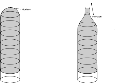
Figure 1: On the left there is an Euclidean section of the near horizon “cigar” geometry of the non-extremal black holes with non-vanishing temperature. On the right there is an Euclidean section of an infinite throat near horizon geometry of the extremal black holes with vanishing temperature.

Euclidean spatial slices of this geometry are illustrated in Figure 1 (analogous to those in [16]. These clearly show the distinct differences in the near horizon geometries of our examples.

To transform this argument into something more rigorous, we will basically repeat the reasoning given in [6] that if extremal black holes have a non-singular geometry and regular values of scalars at the horizon, then such scalars will take the universal values defined by the minimum of the black hole potential. We will use the near horizon geometry with the physical distance coordinate $\omega$ which at the horizon goes to $-\infty$; and, as expected, we will show that source of this universality is attributed to the infinite physical distance to the horizon. An analogous derivation in the non-extremal black holes near horizon geometry with the physical distance coordinate $\rho$, which at the horizon goes to $0$, will show why the horizon values of scalars are non-universal; again, as our reasoning in the previous paragraph suggests, the finite distance to the horizon will prove to be the key.

We start by deriving the equations of motion for the scalar field from the Lagrangian:

$${\cal L}\left(U(\tau),z^{a}(\tau),\bar{z}^{\bar{a}}(\tau)\right)=\left(\left({dU\over d\tau}\right)^{2}+G_{a\bar{a}}{dz^{a}\over d\tau}{d\bar{z}^{\bar{a}}\over d\tau}+e^{2U}V_{BH}(z,\bar{z},p,q)\right)\ .$$ (26)

Varying this action with respect to $\bar{z}^{\bar{a}}$) gives:

$$G_{a\bar{b}}\partial_{\tau}\left(\partial_{\tau}z^{a}\right)+\left(\frac{\partial G_{a\bar{b}}}{\partial\bar{z}^{\bar{a}}}-\frac{\partial G_{a\bar{a}}}{\partial\bar{z}^{\bar{b}}}\right)\partial_{\tau}\bar{z}^{\bar{a}}\partial_{\tau}z^{a}+\frac{\partial G_{a\bar{b}}}{\partial z^{b}}\partial_{\tau}z^{a}\partial_{\tau}z^{b}=e^{2U}\frac{\partial V}{\partial\bar{z}^{\bar{b}}}\ .$$ (27)

If we assume that that the moduli space is a complex Kähler manifold with a Kähler metric $G_{a\bar{b}}$, this simplifies to:

$$\partial_{\tau}\left(\partial_{\tau}z^{a}\right)+\Gamma^{a}_{bc}(z,\bar{z})\partial_{\tau}z^{b}\partial_{\tau}z^{c}=G^{a\bar{b}}e^{2U}\frac{\partial V}{\partial\bar{z}^{\bar{b}}}\ .$$ (28)

Note the the assumption of Kählerity is not essential and the following arguments hold in general. However, for reasons of clarity, we will work in this more constrained situation.

Extremal black holes

The equation of motion (28) for the scalars in the near horizon geometry (24) is given by:

$$\partial_{\tau}\left(\partial_{\tau}z^{a}\right)+\Gamma^{a}_{bc}(z,\bar{z})\partial_{\tau}z^{b}\partial_{\tau}z^{c}=G^{a\bar{b}}e^{2U}\frac{\partial V}{\partial\bar{z}^{\bar{b}}}\ .$$ (29)

We have set $r_{h}=1$ for simplicity. Using $\partial_{\tau}=(-1/\tau)\partial_{\omega}$ and $e^{2U}\rightarrow(r_{h}^{2}/\tau^{2})$ we obtain:

$$(z^{a})^{\prime\prime}+(z^{a})^{\prime}+\Gamma^{a}_{bc}(z^{b})^{\prime}(z^{c})^{\prime}=G^{a\bar{b}}\frac{\partial V}{\partial\bar{z}^{\bar{b}}}\ ,$$ (30)

where $(z^{a})^{\prime}\equiv\partial_{\omega}z^{a}$.

We now argue that the l.h.s. of this expression must vanish identically at the horizon. To see this recall that we are working with the physical distance as our coordinate. Accordingly we expect that the scalar field and all its derivatives with respect to this coordinate will be finite and tend to a definite limit at the horizon. However, if, say, the first derivative of $z^{a}$ tends to some non-zero limit as $\omega\rightarrow-\infty$ then $z^{a}\rightarrow\infty$ as we approach the horizon. Hence, if $z^{a}=constant$ at the horizon, then all the derivatives must be zero there (this extends to higher derivatives by induction).

We are left, then, with the following condition at the horizon:

$$\left.\frac{\partial V}{\partial z^{a}}\right|_{z^{a}_{h}}=0\ .$$ (31)

Since the values of the scalar field that solve this equation are independent of their initial conditions, the horizon is an attractor where the scalar field takes values $z^{a}_{h}\equiv z^{a}_{h}(p,q)$.

Before moving on let’s take a brief detor. It is clear that the analysis above will still hold if the black hole in question is BPS. Of course in this situation we will have the following additional conditions:

$${dU\over d\tau} = e^{U}|Z|\ ,$$ (32)

$${dz^{a}\over d\tau} = e^{U}G^{a\bar{a}}\bar{\cal D}_{\bar{a}}\bar{Z}\ .$$ (33)

These follow immediately from (8), (9) and the 1st order BPS condition. As $\tau\rightarrow-\infty$ (33) can be given in the form (with $r_{h}=1$):

$${dz^{a}\over d\omega}=G^{a\bar{a}}\bar{\cal D}_{\bar{a}}\bar{Z}\ .$$ (34)

Therefore, at the horizon, where the moduli are stabilized, we have:

$${dz^{a}\over d\omega}=G^{a\bar{a}}\bar{\cal D}_{\bar{a}}\bar{Z}=0\ ,$$ (35)

and the number of unbroken supersymmetries is doubled.

Non-extremal black holes

Let’s now examine the equation of motion (28) in the non-extremal near horizon geometry (22):

$$\partial_{\tau}\left(\partial_{\tau}z^{a}\right)+\Gamma^{a}_{bc}(z,\bar{z})\partial_{\tau}z^{b}\partial_{\tau}z^{c}=G^{a\bar{b}}e^{2U}\frac{\partial V}{\partial\bar{z}^{\bar{b}}}\ .$$ (36)

Making the substitutions $e^{2U}\rightarrow(-c^{2}\rho^{2}/r_{h}^{2})$ and $\rho=2e^{c\tau}$ we obtain:

$$\rho(z^{a})^{\prime\prime}+(z^{a})^{\prime}+\rho\Gamma^{a}_{bc}(z^{b})^{\prime}(z^{c})^{\prime}=-\rho G^{a\bar{b}}\frac{\partial V}{\partial\bar{z}^{\bar{b}}}\ .$$ (37)

The prime denotes a derivative with respect to $\rho$. This in turn implies that at $\rho=0$:

$$(z^{a})^{\prime}=0\ .$$ (38)

Substituting this gives us the following equation at the horizon:

$$\left.(z^{a})^{\prime\prime}\right|_{\rho=0}=\left.-G^{a\bar{b}}\frac{\partial V}{\partial\bar{z}^{\bar{b}}}\right|_{z^{a}_{h}}\ .$$ (39)

While at first glance this may seem similar to the equation obtained for the extremal case (30), there is an important difference. Here the coordinate $\rho$ takes the value 0 in the horizon limit. Thus, if we insist that the field and all its derivatives with respect to $\rho$ are finite at the horizon (since it is a physical coordinate), this does not place any further constraints on the $z^{a}$. Indeed such an assertion simply means that the scalar field has a Taylor expansion around $\rho=0$. Thus:

$$\left.-G^{a\bar{b}}\frac{\partial V}{\partial\bar{z}^{\bar{b}}}\right|_{z^{a}_{h}}=A_{2}^{a}\ .$$ (40)

Here $A_{2}^{a}$ are the appropriate coefficients of the Taylor expansion and are, generically, dependent on some initial conditions and not equal to zero. Therefore, for non-extremal black holes the values that the scalar fields take will depend on their initial conditions — there is no attractor.

3 Double-extremal Black Holes

Double-extremal BPS black holes have everywhere-constant moduli, they were studied in [9], [10] and [11]. For example consider Figure 2 where we have plotted the evolution of the dilaton as a function of the coordinate $\rho$ for a particular extremal black hole example from [17]. This coordinate $\rho=-{1\over r}$ is inverse to isotropic coordinate $r$. The double-extremal case corresponds to fixed values of the moduli everywhere in space-time — it is represented by the horizontal line in the plot.

The black hole solution presented in [9] may be supersymmetric if the constant scalars satisfy the equation ${\cal D}Z=0$. However, the solution is valid also when this condition on scalars is not satisfied, as long as $\partial_{a}V=0$. The theory defined by the action (3) has a solution with the extremal Reissner-Nordström geometry and fixed scalars whose values are defined by the condition $\partial_{a}V=0$. As we will show in the next section, this condition is also a consequence of the general attractor equation, and is valid for supersymmetric as well as for non-supersymmetric solutions.

A point that should be stressed here is that in the Reissner-Nordström case there is only one vector field, a graviphoton, and that the vector coupling ${\cal N}_{\Lambda\Sigma}$ in (3) is trivial, with only $\rm\,Im{\cal N}_{00}=-1/2$ for 00 component — there are no axions. In fact, even more general cases double-extremal black holes have a similar metric. There are differences though; the constant scalars now include axions, the matrix ${\cal N}_{\Lambda\Sigma}$ depends on $(p,q)$ and the full solution has a multi-component vector field.

\psfrag{eminus2phi}{$e^{-2z}$}\psfrag{rho}{$\rho$}\includegraphics[width=238.49231pt,height=151.76854pt]{figure13.eps}

Figure 2: Evolution of the dilaton field $e^{-2z}$ for various initial conditions at $\rho=0$ ($r=\infty$) to a common fixed point at $\rho=-\infty$ ($r=0)$ where $\rho=-{1\over r}$. The special case of the horizontal line represents a double-extremal black hole.

We call these black holes double-extremal since they pick up the values of the moduli at infinity that extremize the black hole mass; values that are equal to those at the horizon. There is no energy stored in the scalars, so ${\partial z\over\partial\tau}=0$ everywhere. While for the BPS case ${\cal D}Z=0$ everywhere, the most general conditions are that double-extremal black holes (BPS or otherwise) have Reissner-Nordström geometry and everywhere constant scalars whose values are defined by the critical point of the black hole potential:

$$\partial_{a}V_{BH}=0\ ,\qquad z_{fix}(p,q)=z_{\infty}=z_{h}\ .$$ (41)

Obviously for BPS states (41) is automatically satisified, since $\mathcal{D}_{a}Z=0\Rightarrow\partial_{a}V_{BH}=0$ The double-extremal BPS and non-BPS black hole solution is given in isotropic coordinates by the metric:

$$ds^{2}=e^{2U}dt^{2}-e^{-2U}d\vec{x}^{2}\ .$$ (42)

Where:

$$e^{-U}(r)=1+{\sqrt{A/4\pi}\over r}=1+{M\over r}\ .$$ (43)

With $r^{2}=\vec{x}^{2}$ and the horizon at $r=0$. The constant $A$ is the area of the horizon defined by the value of the potential at the horizon (and, for that matter, the value everywhere else):

$${A\over 4\pi}=V(z_{h},\bar{z}_{h},p,q)=V(z_{\infty},\bar{z}_{\infty},p,q))=V(z_{fix},\bar{z}_{fix},p,q)\ .$$ (44)

The vanishing scalar charges, $\Sigma^{a}$, imply that the the constraint equation at infinity takes the form:

$${A\over 4\pi}=M^{2}(z_{\infty},\bar{z}_{\infty},p,q)=V(z_{fix},\bar{z}_{fix},p,q)\ .$$ (45)

The vector field can be defined by the symplectic doublet $({\cal F}^{\Lambda},\,{\cal G}_{\Lambda})$. Here ${\cal G}_{\Lambda}$ is related to the field ${\cal F}^{\Lambda}$ and its dual $*{\cal F}^{\Lambda}$ as follows: ${\mathcal{G}}_{\Lambda}=(\rm Re\,{\cal N}\,{\cal F})_{\Lambda}-(\rm Im\,{\cal N}\,(*{\cal F}))_{\Lambda}$. The double-extremal solution for the vector fields is given by [9] as:

$${\cal F}^{\Lambda}=e^{2U}{2Q^{\Lambda}\over r^{2}}dt\wedge dr-2P^{\Lambda}d\theta\wedge\sin\theta d\phi\ .$$ (46)

The “dressed” electric and magnetic charges $Q^{\Lambda},P^{\Lambda}$ which are involved in (46) are related to quantized electric and magnetic charges $q_{\Lambda},p^{\Lambda}$ via the moduli dependent vector couplings ${\cal N}_{\Lambda\Sigma}$ as follows:

$$\left(\begin{array}[]{cc}P^{\Lambda}\\ Q^{\Lambda}\end{array}\right)={1\over 2}\left(\begin{array}[]{cc}p^{\Lambda}\\ ((\rm Im\,{\cal N})^{-1}(\rm Re\,{\cal N})p)^{\Lambda}-((\rm Im\,{\cal N})^{-1}q)^{\Lambda}\end{array}\right)\ .$$ (51)

The quantized charges $(p^{\Lambda},q_{\Lambda})$ can be identified with magnetic charges of the doublet $({\cal F}^{\Lambda},\,{\cal G}_{\Lambda})$ via the surface integral:

$$\left(\begin{array}[]{cc}p^{\Lambda}\\ q_{\Lambda}\end{array}\right)=\left(\begin{array}[]{cc}\int{\cal F}^{\Lambda}\\ \int{\cal G}_{\Lambda}\end{array}\right)\ .$$ (52)

Further, we can find the vector couplings as functions of the moduli coordinates. In $\mathcal{N}=2$ supergravities defined by the holomorphic prepotential $F(X)$, the couplings are given in [18] as:

$${\mathcal{N}}_{\Lambda\Sigma}=\overline{F}_{\Lambda\Sigma}+2i\frac{(\mbox{Im}F_{\Lambda\Omega})(\mbox{Im}F_{\Pi\Sigma})z^{\Omega}z^{\Pi}}{(\mbox{Im}F_{\Gamma\Delta})z^{\Gamma}z^{\Delta}}\ .$$ (53)

$F_{\Lambda\Sigma}$ is the second derivative of the prepotential, $\partial_{\Lambda}\partial_{\Sigma}F$ and the special coordinates $z^{\Lambda}$ are defined by $z^{\Lambda}=\frac{X^{\Lambda}}{X^{0}}$, so that $z^{\Lambda}=(1,{X^{a}\over X^{0}})$. For a Calabi-Yau moduli space with $F=D_{abc}{X^{a}X^{b}X^{c}\over X^{0}}$ one finds ([10]):

$$F_{\Lambda\Sigma}=\left(\begin{array}[]{cc}2D_{abc}z^{a}z^{b}z^{c}&-3D_{abc}z^{b}z^{c}\\ -3D_{abc}z^{b}z^{c}&6D_{abc}z^{c}\\ \end{array}\right)\ .$$ (56)

In models where the prepotential $F$ does not exist and only the section $(X^{\Lambda},F_{\Lambda})$ is available, the form of the vector couplings ${\mathcal{N}}_{\Lambda\Sigma}$ can still be found — see [19] for details. In order to completely specify the double-extreme black hole solution at all values of $r$, one also has to give, in addition to the metric and the attractor values of the scalars, the values of the vector fields. We should therefore calculate the vector couplings ${\cal N}_{\Lambda\Sigma}$ at the attractor point for the scalars, providing the values of the “dressed” electric and magnetic charges $Q^{\Lambda}$ and $P^{\Lambda}$. In terms of these charges the fixed value of the black hole potential has a simple expression:

$$V_{fix}(p,q)=(|Z|^{2}+|{\cal D}Z|^{2})_{fix}=\left[-2\rm Im\,{\cal N}_{\Lambda\Sigma}(Q^{\Lambda}Q^{\Sigma}+P^{\Lambda}P^{\Sigma})\right]_{fix}$$ (57)

As we established earlier, since double-extremal black holes have $\partial_{a}V_{BH}=0$ at all points, including for moduli at infinity, the sobriquet is valid for BPS and non-BPS black holes. However, there is a subtle difference — while for the BPS black holes the mass is always at a minimum at infinity, for the non-BPS case one should require (as proposed in [7], [8]) that the second derivative is positive definite .

We will give examples of a BPS and a non-BPS double-extremal black hole in Section 5.2. These examples will be consistent with the those of the solution of the attractor equation in Section 5.1.

4 The Attractor Equation

In this section, we introduce the explicit form of the black hole attractor equation. The equation we find is valid for non-supersymmetric cases as well as for supersymmetric ones. The attractor mechanism in the latter scenario is well known and was developed in [1]-[3].

In the context of type-IIB string theory the electric and magnetic charges of a black hole originate from the self-dual 5-form. Three legs of this 5-form belong to a Calabi-Yau manifold and the other two are in the $4d$ space-time. When the 5-form is integrated over a supersymmetric 3-cycle in the Calabi-Yau manifold it gives a field-strength for the effective ${\mathcal{N}}=2$ supergravity in the $4d$ space-time. The field-strength in $4d$ space-time can, in turn, be integrated over some appropriate 2-cycle to define the electric and magnetic charges. If the 5-form is integrated over the relevant 2-cycle first, we will have a 3-form with regard to the Calabi-Yau.

To set up a normalization in agreement with [3] and [14], we remind ourselves that the graviphoton field strength, $T_{\mu\nu}^{-}$, and the vector multiplet field strength, ${\cal F}^{i-}_{\mu\nu}$, appear in the $4d$ gravitino and chiral gaugino transformations as follows:

$$\delta\psi_{A\mu} = {\cal D}_{\mu}\epsilon_{A}+\epsilon_{AB}T_{\mu\nu}^{-}\gamma^{\nu}\epsilon^{B}\ ,$$

$$\delta\lambda^{aA} = i\gamma^{\mu}\partial_{\mu}z^{a}\epsilon^{A}+{i\over 2}{\cal F}^{a-}_{\mu\nu}\gamma^{\mu\nu}\epsilon_{B}\epsilon^{AB}\ .$$ (58)

$\epsilon^{A}$ is the parameter of the transformation and $\epsilon^{AB}$ is the complete antisymmetric tensor. The central charge and its covariant derivative in ${\mathcal{N}}=2,\ d=4$ supergravity are defined as follows:

$$Z=-{1\over 2}\int_{S_{2}}T^{-}\ ,\qquad Z_{a}\equiv{\cal D}_{a}Z=-{1\over 2}\int_{S_{2}}{\cal F}^{+\bar{a}}G_{a\bar{a}}\ ,$$ (59)

$$\overline{Z}=-{1\over 2}\int_{S_{2}}T^{+}\ ,\qquad\overline{Z}_{\bar{a}}\equiv\overline{\cal D}_{\bar{a}}\overline{Z}=-{1\over 2}\int_{S_{2}}{\cal F}^{-a}G_{a\bar{a}}\ .$$ (60)

In $10d$ supergravity, we start with the self-dual five-form $\mathcal{F}=*{\cal F}$ on the manifold $M_{4}\times K_{6}$. A real conserved field strength is given by the imaginary part of the five-form ${\cal F}^{+}$ such that ${\cal F}_{5}=i({\cal F}^{-}-{\cal F}^{+})=2{\rm Im}\,{\cal F}^{+}$. The appropriate conservation equation for this field strength is $\partial^{\mu}{\cal F}_{\mu\nu\ldots}=0$. We can now define the 3-form in the CY originating from the 5-form ${\cal F}$ as an integral over the 2-cycle:

$$H_{3}={1\over 2}\int_{S_{2}}{\cal F}_{5}={\rm Im}\,\int_{S_{2}}{\cal F}^{+}\ .$$ (61)

Using the Hodge-decomposition for this 3-form (see Appendix C), we can uniquely expand the real 3-form flux as follows:

$$H_{3}={\mathcal{A}}\Omega+\overline{\mathcal{B}}^{\bar{a}}\overline{\mathcal{D}}_{\bar{a}}\overline{\Omega}+{\mathcal{B}}^{a}{\mathcal{D}}_{a}\Omega+\overline{\mathcal{A}}\overline{\Omega}\ .$$ (62)

Here $\Omega=e^{K\over 2}\Omega^{3,0}(K_{6})$ is the covariantly holomorphic three form of the Calabi-Yau and ${\mathcal{A}}$, ${\mathcal{B}}^{a}$, are the coefficients of the expansion. Our approach here is closely related to the one developed in [15] and used for the derivation of the “new attractors” in [12]. We have not included the terms with the second derivative of $\Omega$ since from the special geometry of the moduli space [20] it is known that ${\mathcal{DD}}\Omega$ is not an independent form and, in fact, is related to ${\mathcal{D}}\Omega$ through the Yukawa couplings ($G^{c\bar{d}}$ is the Kähler metric defined on $K_{6}$):

$${\mathcal{D}}_{a}{\mathcal{D}}_{b}\Omega=iC_{abc}G^{c\bar{d}}\overline{{\mathcal{D}}}_{\bar{d}}\overline{\Omega}\ .$$ (63)

The next thing we need to do is to find the coefficients of the expansion (62). Using the expression for the central charge in terms of the covariantly holomorphic three form, namely $Z=\int_{K_{6}}H_{3}\wedge\Omega$, we immediately find that ${\mathcal{A}}=i\overline{Z}$. Following the same procedure, we can also obtain ${\mathcal{B}}^{a}=-iG^{a\bar{b}}\overline{{\mathcal{D}}}_{\bar{b}}\overline{Z}$. Substituting these expressions into the expansion, we obtain (in agreement with [3], [12] and [14]) the Hodge-decomposition of the 3-form flux as:

$$H_{3}=2{\rm Im}\left[\,Z\,\bar{\Omega}_{3}+\overline{\mathcal{D}}_{\bar{a}}\overline{Z}G^{\bar{a}a}{\mathcal{D}}_{a}{\Omega}_{3}\right]={\rm Im}\,\int_{S_{2}}{\cal F}^{+}\ .$$ (64)

Notice that this relation is valid at any arbitrary point of the moduli space. After integrating over the 3-cycles we can rewrite the above relation in terms of the integer charges:

$$h=2\mbox{Im}\Big{[}\ Z\overline{\Pi}+G^{\bar{a}b}\overline{\mathcal{D}}_{\bar{a}}\overline{Z}\ {{\mathcal{D}}}_{b}{\Pi}\ \Big{]}\ .$$ (65)

$h=(p^{\Lambda},q_{\Lambda})$ is the set of magnetic and electric charges and $\Pi$ is the covariantly holomorphic period vector. Clearly, at supersymmetric extrema (where ${\mathcal{D}}_{a}Z=0$), this gives a simple ([1]-[4]) algebraic expression:

$$h=2\mbox{Im}[Z\overline{\Pi}]\ .$$ (66)

In more general case, we can use the minimization condition of the effective potential of black hole $\partial V_{BH}=0$ which is equivalent to ([6]):

$$2({\mathcal{D}}_{a}Z)\bar{Z}+iC_{abc}G^{b\bar{d}}G^{c\bar{e}}\bar{\mathcal{D}}_{\bar{d}}\bar{Z}\bar{\mathcal{D}}_{\bar{e}}\bar{Z}=0\ .$$ (67)

This readily gives:

$${\mathcal{D}}_{a}Z=-i\frac{C_{abc}G^{b\bar{d}}G^{c\bar{e}}\bar{\mathcal{D}}_{\bar{d}}\bar{Z}\bar{\mathcal{D}}_{\bar{e}}\bar{Z}}{2\bar{Z}}\ .$$ (68)

Using the special geometry relation ${\mathcal{D}}_{a}{\mathcal{D}}_{b}Z=iC_{abc}G^{c\bar{d}}\bar{\mathcal{D}}_{\bar{d}}\bar{Z}$ in the above equation and substituting into the result for (65), we find the following equation:

$$h=2\mbox{Im}\left[Z\overline{\Pi}-\frac{(\overline{\mathcal{D}}_{\bar{a}}\overline{\mathcal{D}}_{\bar{b}}\overline{Z})G^{\bar{a}{c}}G^{\bar{b}{d}}{\mathcal{D}}_{{c}}{Z}{{\mathcal{D}}}_{d}{\Pi}}{2{Z}}\right]\ .$$ (69)

The replacements made above are only valid in case that $Z\neq 0$.

This is the general form of the attractor equation, valid both for supersymmetric and non-supersymmetric cases. We claim that solving the above equation to find the moduli at horizon of the black hole is equivalent to the minimization of the potential.

That (69) was derived using a type-IIB string theory compactified on a CY manifold is somewhat auxiliary to the result. It is an equation that is valid for the general case of 4d non-BPS black holes (as defined in Section 2) in the framework of special geometry. This is analogous to the situation that took place for the BPS black hole attractor equation. While in [2] the equation $h=2\mbox{Im}[Z\overline{\Pi}]$ was derived string theory compactified on a CY manifold, in [3] the derivation was extended to the general case of special geometry. Thus our new non-BPS black hole attractor equation is valid for any non-BPS black holes in special geometry, in particular when they are derived from type-IIA string theory. In the next section, we explicitly solve (69) for specific situations and find the value of the moduli at the horizon of the black hole and compare our results with minimizing the effective potential.

Before we move on to the next section, we point out that care should be taken with the precise meaning of (69). We use the symbol ${\mathcal{D}}$ to denote the fully covariant derivative:

$${\mathcal{D}}=\partial+x(\partial K)+\Gamma\ .$$ (70)

where $x$ denotes the Kähler weight of the object that the covariant derivative acts on and $\Gamma$ denotes the Christoffel symbol(s) of the Levi-Civita connection of the Kähler metric. The Kähler weight $x$ of an object ${\mathcal{O}}$ is determined by its transformation law under Kähler transformation. When $K\rightarrow K+f(z)+\bar{f}(\bar{z})$, the object ${\mathcal{O}}$ transforms as ${\mathcal{O}}\rightarrow e^{x(f(z)-\bar{f}(\bar{z}))}{\mathcal{O}}$, see e. g. [21]. The Kähler weights for the central charge $Z$ and its conjugate, are $\frac{1}{2}$ and $-\frac{1}{2}$ respectively. It follows from this that the superpotential $W=e^{-K/2}Z$ has a covariant derivative ${\mathcal{D}}W=e^{-K/2}\left(\partial+{1\over 2}(\partial K)\right)Z=\partial W+\partial KW$ and the conjugate has a vanishing covariant derivative ${\mathcal{D}}\overline{W}=e^{-K/2}\left(\partial-{1\over 2}(\partial K)\right)\overline{Z}=\partial\overline{W}=0$. Notice that this definition of covariant derivative is different from the derivative $\nabla$ used in [8], which does not include Christoffel symbols. Of course the two operations are identical when acting on scalar quantities (such as the effective potential and the superpotential), but the distinction becomes important once we consider second derivatives. Somewhat more detail on this issue (especially with regards to the differences between the above quoted expression for the extremal condition and that used in [8]) can be found in Appendix B.

5 Solving the Attractor Equation

In this section, we consider three examples, explicitly solve the attractor equation for them and extract the values of the moduli at the horizon (the attractor point). The first of these are black hole attractors in the framework of type-IIA string compactification, where we take the internal space to be a Calabi-Yau manifold whose volume is large. Next we consider a double-extremal example, in the same background. In the final example, we study the mirror quintic manifold in type-IIB, at the vicinity of the Gepner point. In each case, we first solve the attractor equation directly to find the moduli at horizon and then we compare our results with those from the minimization of the effective potential presented in [8].

5.1 Large Volume Calabi-Yau in the Absence of D6-brane

Here we solve the attractor equation directly for black hole attractors in the framework of type-IIA string theory compactifications, in which the internal space is a Calabi-Yau manifold with large volume. The BPS attractor equation for this system was solved in [11] and the moduli at horizon in the non-BPS case were found in [8] by minimizing the effective potential of the black hole.

In the low-energy limit of ${\mathcal{N}}=2$ theory compactified on a CY three-fold with $h^{1,1}(K_{6})=N$, the superpotential takes the following form:

$$W=q_{0}+q_{a}z^{a}-3D_{abc}p^{a}z^{b}z^{c}\ ,$$ (71)

in which $q_{0},q_{a},$ and $p^{a}$ are D0, D2 and D4-brane charges respectively. For simplicity, we assume that there is no D6-brane in this setup, $p^{0}=0$. The Kähler potential is then given by:

$$K=-\ln\Big{(}-iD_{abc}\big{(}z^{a}-\bar{z}^{a}\big{)}\big{(}z^{b}-\bar{z}^{b}\big{)}\big{(}z^{c}-\bar{z}^{c}\big{)}\Big{)}\ .$$ (72)

Also, we assume that there is no D2-brane, namely $q_{a}=0$. Before jumping into the task of calculating the terms which are involved in (69), it is prudent to obtain the form of the solution. By solving (69), we find $z^{a}$ as a function of charges and for the present situation, the only charges are those associated with the D0-brane and D4-brane, namely $q_{0}$ and $p^{a}$. Therefore, it is quite clear that the most general symplectic vector which can be constructed from $q_{0}$ and $p^{a}$ has the form $z^{a}=ip^{a}t(q_{0},D)$, where we have defined $D=D_{abc}p^{a}p^{b}p^{c}$. We can set all the $z^{a}$ to be purely imaginary since the superpotential is quadratic with respect to them. This implies that $t(q_{0},D)$ is a real function.

First term of The Attractor Equation

Now, we calculate the terms of r.h.s. of (69). We know that:

$$\ Z=e^{K/2}W\ ,\ \ \Pi=e^{K/2}\left(\begin{array}[]{c}1\\ z^{a}\\ F_{0}\\ F_{a}\\ \end{array}\right)\ .$$ (77)

Thus, considering the fact that the Kähler potential is real, we can write the first term of the r.h.s. of (69) as:

$$Z\overline{\Pi}=e^{K}W\left(\begin{array}[]{c}1\\ \bar{z}^{a}\\ \bar{F}_{0}\\ \bar{F}_{a}\\ \end{array}\right)\ .$$ (82)

$F_{a}=\partial_{a}F=\partial_{a}(D_{bcd}z^{b}z^{c}z^{d})=3D_{abc}z^{b}z^{c}$ and $F_{0}=\partial_{0}F=\partial_{0}(\frac{D_{bcd}X^{b}X^{c}X^{d}}{X^{0}})=-D_{abc}z^{a}z^{b}z^{c}$. Substituting the general form of $z^{a}=ip^{a}t$ into the above expression, we get:

$$\overline{F_{a}}=3D_{abc}(-ip^{b}t)(-ip^{c}t)=-3D_{a}t^{2}\ ,$$ (83)

$$\overline{F_{0}}=-D_{abc}(-ip^{a}t)(-ip^{b}t)(-ip^{c}t)=-iDt^{3}\ ,$$ (84)

where $D_{a}=D_{abc}p^{b}p^{c}$. Using $M=D(2it)^{3}=-8iDt^{3}$ (see (98)), we easily find $e^{K}=\frac{i}{M}=\frac{-1}{8Dt^{3}}$. Therefore, the first term of the r.h.s. of (69) reads:

$$2(Z\overline{\Pi})=-\frac{W}{4Dt^{3}}\left(\begin{array}[]{c}1\\ -ip^{c}t\\ -iDt^{3}\\ -3D_{c}t^{2}\\ \end{array}\right)\ .$$ (89)

Notice that $c$ is a free index and runs over 1 to $h^{1,1}=N$. Substituting the general form of $z^{a}=ip^{a}t$ for (71), the superpotential becomes $W=(q_{0}+3Dt^{2})$ — this is clearly real. Finally, the imaginary part of (89) gives the first term of the r.h.s. of the attractor equation:

$$2\mbox{Im}(Z\overline{\Pi})=\frac{W}{4Dt^{2}}\left(\begin{array}[]{c}0\\ p^{c}\\ Dt^{2}\\ 0\\ \end{array}\right)\ .$$ (94)

Second Term of The Attractor Equation

In order to evaluate the second term of the attractor equation, we need to compute the first and second covariant derivatives of the superpotential as well as the first covariant derivative of the period vector.

Following the notion of [8], the covariant derivative of the superpotential is:

$${\mathcal{D}}_{a}W=(\partial_{a}+(\partial_{a}K))W=-6D_{ab}z^{b}-\frac{3M_{a}}{M}W\ .$$ (95)

Here $D_{ab}=D_{abc}p^{c}$ and $M_{ab}$, $M_{a}$, and $M$ are defined as:

$$M_{ab}=D_{abc}(z^{c}-\bar{z}^{c})\ ,$$ (96)

$$M_{a}=D_{abc}(z^{b}-\bar{z}^{b})(z^{c}-\bar{z}^{c})\ ,$$ (97)

$$M=D_{abc}(z^{a}-\bar{z}^{a})(z^{b}-\bar{z}^{b})(z^{c}-\bar{z}^{c})\ .$$ (98)

If we again substitute the general form of $z^{a}=ip^{a}t$ into the above expressions, we obtain $M_{ab}=2iD_{ab}t$, $M_{a}=-4D_{a}t^{2}$, and $M=-8iDt^{3}$. Then, the covariant derivative of the superpotential reads:

$${\mathcal{D}}_{a}W=-3itD_{a}\Big{(}2-\frac{W}{2Dt^{2}}\Big{)}\ \ \ ,\ \ \ \overline{\mathcal{D}}_{\bar{a}}\overline{W}=+3itD_{a}\Big{(}2-\frac{W}{2Dt^{2}}\Big{)}\ .$$ (99)

The second covariant derivative of the superpotential is:

$${\mathcal{D}}_{a}{\mathcal{D}}_{b}W=(\partial_{a}+(\partial_{a}K)){\mathcal{D}}_{b}W-\Gamma^{d}_{ab}{\mathcal{D}}_{d}W\ ,$$ (100)

with the Christoffel symbols of the Kähler metric given by $\Gamma^{d}_{ab}=G^{d\bar{e}}\partial_{a}G_{\bar{e}b}$. Expressions for the metric and inverse metric can be found in [8]:

$$G_{a\bar{b}} = \frac{3}{M}\left(2M_{ab}-\frac{3}{M}M_{a}M_{b}\right)$$ (101)

$$G^{a\bar{b}} = \frac{M}{6}\left(M^{ab}-\frac{3}{M}(z^{a}-\bar{z}^{a})(z^{b}-\bar{z}^{b})\right)\ .$$ (102)

These, in turn, imply that the Christoffel symbols take the following form:

$$\Gamma^{d}_{ab}=M^{de}D_{eab}-\frac{3}{M}\Big{(}M_{a}\delta^{d}_{b}+M_{b}\delta^{d}_{a}-M_{ab}(z^{d}-\bar{z}^{d})\Big{)}\ .$$ (103)

Combining (99) and (103), we get:

$$\Gamma^{d}_{ab}{\mathcal{D}}_{d}W=-12D_{ab}+18\frac{D_{a}D_{b}}{D}+\frac{3W}{2Dt^{2}}\big{(}2D_{ab}-3\frac{D_{a}D_{b}}{D}\big{)}\ .$$ (104)

We can also compute the first piece of (100):

$$(\partial_{a}+(\partial_{a}K)){\mathcal{D}}_{b}W=-6D_{ab}+18\frac{D_{a}D_{b}}{D}+\frac{3W}{2Dt^{2}}\big{(}D_{ab}-3\frac{D_{a}D_{b}}{D}\big{)}\ .$$ (105)

After all this, we obtain the second covariant derivative of the superpotential:

$${\mathcal{D}}_{a}{\mathcal{D}}_{b}W=3D_{ab}\Big{(}2-\frac{W}{2Dt^{2}}\Big{)}\ .$$ (106)

The last thing we need to compute is the covariant derivative of the period vector. Using the expression for the period vector (77), we now find its covariant derivative:

$${\mathcal{D}}_{d}\Pi=e^{K/2}{\mathcal{D}}_{d}\left(\begin{array}[]{c}1\\ z^{c}\\ F_{0}\\ F_{c}\\ \end{array}\right)=e^{K/2}\left(\begin{array}[]{c}\partial_{d}K\\ \delta^{c}_{d}+\partial_{d}K\ z^{c}\\ -3D_{def}z^{e}z^{f}-\partial_{d}KD_{efh}z^{e}z^{f}z^{h}\\ 6D_{cde}z^{e}+3\partial_{d}K\ D_{cef}z^{e}z^{f}\\ \end{array}\right)\ .$$ (115)

We can easily see that $\partial_{d}K=-3\frac{M_{d}}{M}=\frac{3iD_{d}}{2Dt}$. Substituting this result in the above expression, we get:

$${\mathcal{D}}_{d}\Pi=e^{K/2}\left(\begin{array}[]{c}\frac{3}{2}i\frac{D_{d}}{D}\frac{1}{t}\\ \delta^{c}_{d}-\frac{3}{2}p^{c}\frac{D_{d}}{D}\\ \frac{3}{2}D_{d}t^{2}\\ 6iD_{cd}t-\frac{9}{2}i\frac{D_{d}D_{c}}{D}t\\ \end{array}\right)\ .$$ (120)

Combining the above result with (99), (101) and (106), we get the second term of the attractor equation:

$$2\mbox{Im}\Bigg{[}\frac{(\overline{{\mathcal{D}}}_{\bar{a}}\overline{{\mathcal{D}}}_{\bar{b}}\bar{Z})G^{\bar{a}c}G^{\bar{b}d}{\mathcal{D}}_{c}Z{\mathcal{D}}_{d}\Pi}{2Z}\Bigg{]}=-\frac{Dt^{2}}{2W}(-2+\frac{W}{2Dt^{2}})(4-\frac{W}{Dt^{2}})\left(\begin{array}[]{c}0\\ -p^{c}\\ 3Dt^{2}\\ 0\\ \end{array}\right)\ .$$ (125)

Adding the Two Terms Up

Now that we have the two terms of the r.h.s. of the attractor equation, we can form the equation and solve it in order to find $t(q_{0},D)$. We know $h=(p^{\Lambda},q_{\Lambda})$ is the set of charges and for this setup we have:

$$h=\left(\begin{array}[]{c}0\\ p^{c}\\ q_{0}\\ 0\\ \end{array}\right)\ .$$ (130)

If we define the new variable $Y=\frac{W}{Dt^{2}}$, then we can write the attractor equation (69) in the following way:

$$\left(\begin{array}[]{c}0\\ p^{c}\\ (Y-3)Dt^{2}\\ 0\\ \end{array}\right)=\left(\begin{array}[]{c}0\\ \Big{(}\frac{1}{4}Y-\frac{1}{2Y}\big{(}-2+\frac{1}{2}Y\big{)}(4-Y)\Big{)}p^{c}\\ \Big{(}\frac{1}{4}Y+\frac{3}{2Y}\big{(}-2+\frac{1}{2}Y\big{)}(4-Y)\Big{)}Dt^{2}\\ 0\\ \end{array}\right)\ ,$$ (139)

in which we have substituted $q_{0}$ by $q_{0}=W-3Dt^{2}=(Y-3)Dt^{2}$. Now, we find that both non-vanishing rows of the above matrix equation lead to the following equation for $Y$:

$$(Y-4)(Y-2)=0\ .$$ (140)

The solution $Y=4$, which corresponds to the supersymmetric solution (because ${\mathcal{D}}_{a}W=0$ at $Y=4$, see (99)), leads us to the result $t=\sqrt{\frac{q_{0}}{D}}$. However, the solution $Y=2$, corresponding to the non-supersymmetric solution (${\mathcal{D}}_{a}W\neq 0$ at $Y=2$), gives us $t=\sqrt{-\frac{q_{0}}{D}}$.

Minimization of The Effective Potential

In the previous section, we explicitly solved the attractor equation and found the moduli at the horizon (the attractor point) of the black hole. In [8], however, the moduli at horizon is found by the minimization of the effective potential of the black hole. Here we see that these approaches are equivalent.

Minimization of the effective potential leads to the following equation:

$$\partial_{a}V_{eff}={\mathcal{D}}_{a}\Big{(}|Z|^{2}+|{\mathcal{D}}Z|^{2}\Big{)}=e^{K}\Big{(}g^{b\bar{c}}({\mathcal{D}}_{a}{\mathcal{D}}_{b}W)\bar{{\mathcal{D}}}_{\bar{c}}\overline{W}+2({\mathcal{D}}_{a}W)\overline{W}\Big{)}=0\ .$$ (141)

Using the general form of $z^{a}=ip^{a}t$, the equation governing $t$ takes the following form:

$$(q_{0}-t^{2}D)(q_{0}+t^{2}D)=0\ .$$ (142)

The solution $t_{1}=\sqrt{\frac{q_{0}}{D}}$ is the supersymmetric one (where ${\mathcal{D}}_{a}W$ vanishes) and $t_{2}=\sqrt{-\frac{q_{0}}{D}}$ is the non-supersymmetric one (where ${\mathcal{D}}_{a}W\neq 0$). Thus we confirm that the two procedures lead to the same answer.

5.2 An Example of the Non-BPS Double-extremal Black Hole

In this subsection, we will first review an example of a double-extremal black hole given in [11]. It corresponds to a special case of the model studied in Sec. 5.1 when there are only 3 moduli coordinates $z^{1},z^{2},z^{3}$. The only non-vanishing component of $D_{abc}$ is $D_{123}=-1/6$ and therefore $D=-p^{1}p^{2}p^{3}$.

As explained in Section 3, double-extremal black holes are Reissner-Nordström type solutions of the theory defined by action (3) where the moduli fields $z^{a},\bar{z}^{\bar{a}}$ take constant values. The values of the moduli at the horizon of the black hole are determined by solving the attractor equation (or equivalently by finding the critical points of the black hole potential). Therefore, the constant values for double-extremal black holes are defined by the solution of the attractor equation.

Double-extremal BPS Black Hole

As shown in [9]-[11] the 4-dimensional metric, in the double-extremal limit, defines an extreme Reissner-Nordström metric $ds_{4}^{2}=e^{2U}\ dt^{2}-e^{-2U}d\vec{x}^{2}$, where:

$$e^{-2U}=\sqrt{H_{0}D_{abc}H^{a}H^{b}H^{c}}=\Big{(}1+{M\over r}\Big{)}^{2}\ ,\qquad M^{2}=2\sqrt{q_{0}D}\ .$$ (143)

Here the harmonic (i.e. $\partial_{i}\partial_{i}H_{0}=\partial_{i}\partial_{i}H^{a}=0$) functions are given by:

$$H_{0}=\sqrt{2}q_{0}\Big{(}k+\frac{1}{r}\Big{)}\ ,\ \ \ H^{1}=-\sqrt{2}p^{1}\Big{(}k+\frac{1}{r}\Big{)}\ ,$$

$$H^{2}=\sqrt{2}p^{2}\Big{(}k+\frac{1}{r}\Big{)}\ ,\ \ \ H^{3}=\sqrt{2}p^{3}\Big{(}k+\frac{1}{r}\Big{)}\ .$$ (144)

$k^{-4}=-4q_{0}p^{1}p^{2}p^{3}$ and $r=|\vec{x}|$. It is assumed that $q_{0}D=-q_{0}p^{1}p^{2}p^{3}>0$. The constant values of the three moduli are:

$$z^{1}=i\sqrt{\frac{H_{0}H^{1}}{H^{2}H^{3}}}=i\,p^{1}\sqrt{\frac{q_{0}}{D}}\ ,$$ (145)

$$z^{2}=i\sqrt{\frac{H_{0}H^{2}}{H^{1}H^{3}}}=i\,p^{2}\sqrt{\frac{q_{0}}{D}}\ ,$$ (146)

$$z^{3}=i\sqrt{\frac{H_{0}H^{3}}{H^{1}H^{2}}}=i\,p^{3}\sqrt{\frac{q_{0}}{D}}\ .$$ (147)

It is evident that all of the above only depend on the electric charge $q_{0}$ and the magnetic charges $p^{1}$, $p^{2}$, and $p^{3}$. Moreover, as mentioned in Section 3, the solution for the four vector fields is given by (46). For this example, we need to introduce the values of the dressed charges and of $M$. To do this, one first has to find the vector couplings. Using (53) we obtain ($t=\sqrt{q_{0}/D}$):

$${\mathcal{N}}_{\Lambda\Sigma}=\left(\begin{array}[]{cc}iDt^{3}&0\\ 0&-6iD_{ab}t+9it\frac{D_{a}D_{b}}{D}\\ \end{array}\right)\ .$$ (150)

The fact that the above matrix has no real entries implies that we do not have any axions for this example, as expected. Using (51) we simply find the values of the dressed electric and magnetic charges as $P^{0}=0$, $P^{a}={1\over 2}p^{a}$, $Q^{0}={1\over 2t}$ and $Q^{a}=0$. Also we have $M^{2}=2\sqrt{q_{0}D}=-2(\mbox{Im}\,{\cal N}_{\Lambda\Sigma})(Q^{\Lambda}Q^{\Sigma}+P^{\Lambda}P^{\Sigma})$. In addition to the constant values of the scalar fields, one also has to find the values of the the vector fields. Using (46), the electric and magnetic fields are given in terms of harmonic functions $H_{0}$, $H^{1}$, $H^{2}$, and $H^{3}$ as:

$${\cal F}^{0}_{i0}=\partial_{i}\psi^{0}\ ,\qquad{\cal G}_{a\,i0}=\partial_{i}\chi_{a}\ .$$ (151)

The electric and magnetic potentials are proportional to the inverses of the harmonic functions:

$$\psi^{0}=\frac{1}{\sqrt{2}}(H_{0})^{-1}\ ,\qquad\chi_{a}=\frac{1}{\sqrt{2}}(H^{a})^{-1}\ .$$ (152)

Double-extremal Non-BPS Black Hole

Now we wish to consider the double-extremal black hole for the non-supersymmetric case. In the previous section, we explicitly solved the attractor equation (69) to find the values of moduli coordinates at the horizon of the black hole. In the general setup, we had $N$ moduli coordinates, an electric charge $q_{0}$ and magnetic charges $p^{a}$. Comparing supersymmetric and non supersymmetric solutions, we immediately realize that in order to obtain the double-extremal black hole in the non-BPS case one only needs to substitute $q_{0}$ by $-q_{0}$ in the supersymmetric double-extremal black hole solution with $-q_{0}D>0$.

This leads to the following expressions for the harmonic functions:

$$\tilde{H}_{0}=-\sqrt{2}q_{0}\Big{(}\tilde{k}+\frac{1}{r}\Big{)}\ ,\ \ \ \tilde{H}^{1}=-\sqrt{2}p^{1}\Big{(}\tilde{k}+\frac{1}{r}\Big{)}\ ,$$

$$\tilde{H}^{2}=\sqrt{2}p^{2}\Big{(}\tilde{k}+\frac{1}{r}\Big{)}\ ,\ \ \ \tilde{H}^{3}=\sqrt{2}p^{3}\Big{(}\tilde{k}+\frac{1}{r}\Big{)}\ ,$$ (153)

where, in this case, $\tilde{k}^{-4}=+4q_{0}p^{1}p^{2}p^{3}$. In terms of these harmonic functions the metric is the same as in (143). The scalars, again in terms of new harmonic functions, are the same as in (145). This corresponds to changing $q_{0}$ to $-q_{0}$ and we get $\tilde{M}^{2}=2\sqrt{-q_{0}D}$.

Therefore, considering the BPS solution (145), the constant values of the three moduli coordinates for the non-BPS black hole are given by:

$$\tilde{z}^{1}=i\sqrt{\frac{\tilde{H}_{0}\tilde{H}^{1}}{\tilde{H}^{2}\tilde{H}^{3}}}=i\,p^{1}\sqrt{\frac{-q_{0}}{D}}\ ,$$ (154)

$$\tilde{z}^{2}=i\sqrt{\frac{\tilde{H}_{0}\tilde{H}^{2}}{\tilde{H}^{1}\tilde{H}^{3}}}=i\,p^{2}\sqrt{\frac{-q_{0}}{D}}\ ,$$ (155)

$$\tilde{z}^{3}=i\sqrt{\frac{\tilde{H}_{0}\tilde{H}^{3}}{\tilde{H}^{1}\tilde{H}^{2}}}=i\,p^{3}\sqrt{\frac{-q_{0}}{D}}\ .$$ (156)

From (152) we can also find the values of the electric and magnetic potentials; in terms of harmonic functions these are:

$$\tilde{\cal F}^{0}_{i0}=\partial_{i}\tilde{\psi}^{0},\qquad\tilde{\cal G}_{a\,i0}=\partial_{i}\tilde{\chi}_{a}\ .$$ (157)

The electric and magnetic potentials are related to the inverse of harmonic functions in the following way:

$$\tilde{\psi}^{0}=\frac{1}{\sqrt{2}}(\tilde{H}_{0})^{-1}\qquad\tilde{\chi}_{a}=\frac{1}{\sqrt{2}}(\tilde{H}^{a})^{-1}\ .$$ (158)

5.3 Mirror Quintic

In this section, we consider black holes in the framework of type-IIB string theory compactified on mirror quintic Calabi-Yau 3-folds. We closely follow the notation of [8] and [22]. For a quintic hypersurface in $P^{4}$, the mirror quintic $M$ is obtained by the following quotient([23]):

$$M=\Big{(}\sum_{i=1}^{5}Z_{i}^{5}-5\psi\prod_{i=1}^{5}Z_{i}\Big{)}\Big{/}(Z_{5})^{3}\ ,$$ (159)

where $\psi$ is a complex coefficient. The Hodge numbers of the mirror quintic Calabi-Yau are $h^{1,1}(M)=101$ and $h^{2,1}(M)=1$. In IIB theory, the vector multiplet moduli space which corresponds to the deformations of the complex structure is parameterized by $\psi$ and is one dimensional. In terms of homology there are, in general, $2(h^{2,1}(M)+1)$ nontrivial 3-cycles $\{A^{a},B_{a}\}$. From the holomorphic 3-form $\Omega$ of the Calabi-Yau manifold, we can find the special coordinates $z^{a}$ of the vector multiplet moduli space and the prepotential $F$:

$$\int_{A^{a}}\Omega=z^{a}\ \ ,\ \ \int_{B_{a}}\Omega=\partial_{a}F\ .$$ (160)

The Kähler potential and the superpotential are then given by:

$$K=-\log(-i\Pi^{{\dagger}}\cdot\Sigma\cdot\Pi)\ \ ,\ \ W=h^{T}\cdot\Sigma\cdot\Pi\ ,$$ (161)

where $\Sigma$ is a matrix given in Appendix D, $h=(p^{a},q_{a})$ is the set of electric and magnetic charges and $\Pi$ is the period function. We notice that both $h$ and $\Pi$ are four dimensional column vectors. Now, we want to solve the attractor equation ((69)) for the case of mirror quintic in the vicinity of the Gepner point ($\psi=0$) at which the holomorphic 3-form of the Calabi-Yau is well known as a power series ([23]). In this limit, we find all ingredients of the attractor equation as a series in terms of $\psi$ and then we only keep linear terms. The Kähler potential and the superpotential are then expressed as:

$$K=C_{0}-\log\Big{(}1+(2-\sqrt{5})\frac{c_{1}^{2}}{c_{0}^{2}}|\psi|^{2}-(2-\sqrt{5})\frac{c_{2}^{2}}{c_{1}^{2}}|\psi|^{4}+\cdots\Big{)}\ ,$$ (162)

$$W=\frac{1}{25}\Big{(}\frac{2\pi i}{5}\Big{)}^{3}\Big{(}c_{0}n\cdot p_{0}+c_{1}n\cdot p_{1}\psi+c_{2}n\cdot p_{2}\psi^{2}+\cdots\Big{)}\ .$$ (163)

The constants $C_{0}$, $c_{i}$ and the column vectors $p_{i}$ are defined in Appendix D. $n$ is a column vector which is related to the charges by $n=5\tilde{m}h$, where matrix $\tilde{m}$ can be found in appendix [C]. From the Kähler potential, it is straightforward to calculate the Kähler metric and the Christoffel symbols of the Levi-Civita connection associated with this metric:

$$G^{\psi\bar{\psi}}=-\frac{c_{0}^{2}}{c_{1}^{2}(2-\sqrt{5})}\Bigg{[}1+\Big{(}2(2-\sqrt{5})\frac{c_{1}^{2}}{c_{0}^{2}}+4\frac{c_{2}^{2}}{c_{1}^{2}}\Big{)}|\psi|^{2}+\cdots\Bigg{]}\ ,$$ (164)

$$\Gamma^{\psi}_{\psi\psi}=-2\Big{(}\ (2-\sqrt{5})\frac{c_{1}^{2}}{c_{0}^{2}}+2\frac{c_{2}^{2}}{c_{1}^{2}}\ \Big{)}\bar{\psi}\ .$$ (165)

Now we are able to compute the ingredients of the attractor equation. The covariant derivatives of the superpotential are given by:

$${\mathcal{D}}_{\psi}W=\frac{1}{25}\Big{(}\frac{2\pi i}{5}\Big{)}^{3}\Big{(}c_{1}n\cdot p_{1}+2c_{2}n\cdot p_{2}\psi-\frac{c_{1}^{2}}{c_{0}^{2}}(2-\sqrt{5})c_{0}n\cdot p_{0}\bar{\psi}\Big{)}\ ,$$ (166)

$${\mathcal{D}}_{\psi}{\mathcal{D}}_{\psi}W=\frac{2}{25}\Big{(}\frac{2\pi i}{5}\Big{)}^{3}\Big{(}c_{2}n\cdot p_{2}+3c_{3}n\cdot p_{3}\psi+2\frac{c_{2}^{2}}{c_{1}}n\cdot p_{1}\bar{\psi}\Big{)}\ .$$ (167)

The period vector in terms of $\psi$ is:

$$\Pi=\frac{1}{5}\Big{(}\frac{2\pi i}{5}\Big{)}^{3}\Big{(}c_{0}\tilde{m}p_{0}+c_{1}\tilde{m}p_{1}\psi+c_{2}\tilde{m}p_{2}\psi^{2}+\cdots\Big{)}\ .$$ (168)

For the covariant derivative of the period vector, we get:

$${\mathcal{D}}_{\psi}\Pi=\frac{1}{5}\Big{(}\frac{2\pi i}{5}\Big{)}^{3}\Big{(}c_{1}\tilde{m}p_{1}+2c_{2}\tilde{m}p_{2}\psi-(2-\sqrt{5})\frac{c_{1}^{2}}{c_{0}}\tilde{m}p_{0}\bar{\psi}\Big{)}\ .$$ (169)

So far, we have computed all the ingredients of the r.h.s. of the attractor equation (69) for the mirror quintic. The only thing we need is the l.h.s. of (69), namely the charges which should be expressed in terms $n$. This is given by:

$$h=\left(\begin{array}[]{c}p^{a}\\ q_{a}\\ \end{array}\right)=\frac{1}{5}\left(\begin{array}[]{c}-20n_{1}\\ 2(4n_{1}-n_{2})\\ 11n_{1}\\ -4n_{1}+n_{2}\\ \end{array}\right)\ ,$$ (176)

in which we assumed that vector $n$ has the form $n=(n_{1},n_{2},n_{2},n_{1})$. This assumption is not necessary but it makes the calculations easier. Specifically, one can see that such an assumption ensures all the $n\cdot p_{i}$ are real. Next we form the attractor equation and ignore all quadratic and higher order terms in $\psi$. Then, we have:

$$2\mbox{Im}\Bigg{[}Z\overline{\Pi}-(G^{\psi\bar{\psi}})^{2}\frac{(\overline{{\mathcal{D}}}_{\bar{\psi}}\overline{{\mathcal{D}}}_{\bar{\psi}}{\overline{Z}}){\mathcal{D}}_{\psi}Z{\mathcal{D}}_{\psi}\Pi}{2Z}\Bigg{]}-h=0=N_{1}+N_{2}\psi\ .$$ (177)

$N_{1}$ is expressed in the following way:

$$N_{1}=-h+\frac{2}{5\sqrt{2+2\sqrt{5}}}\ \tilde{m}\Big{(}(n\cdot p_{0})\mbox{Im}\bar{p}_{0}-\frac{1}{(2-\sqrt{5})^{2}}\frac{c_{0}c_{2}}{c_{1}^{2}}\frac{(n\cdot p_{1})^{2}}{n\cdot p_{0}}\mbox{Im}p_{1}\Big{)}\ ,$$ (178)

For $N_{2}$ we obtain (assuming $\psi$ is real):

$$N_{2}=\frac{2}{5\sqrt{2+2\sqrt{5}}}\ \tilde{m} \Bigg{[} \frac{c_{1}}{c_{0}}\Big{(}(n\cdot p_{1})\mbox{Im}\bar{p}_{0}+(n\cdot p_{0})\mbox{Im}\bar{p}_{1}\Big{)}-\frac{2}{(2-\sqrt{5})^{2}}\frac{c_{0}c_{2}^{2}}{c_{1}^{3}}\frac{(n\cdot p_{1})^{2}}{n\cdot p_{0}}\mbox{Im}(p_{1}+p_{2})$$ (179)

$$+\frac{1}{(2-\sqrt{5})^{2}}\frac{c_{2}}{c_{1}}\frac{(n\cdot p_{1})^{3}}{(n\cdot p_{0})^{2}}\mbox{Im}p_{1}-\frac{3}{(2-\sqrt{5})^{2}}\frac{c_{0}c_{3}}{c_{1}^{2}}(n\cdot p_{1})\mbox{Im}p_{1}$$

$$+\frac{1}{(2-\sqrt{5})}\frac{c_{2}}{c_{1}}\Big{(}(n\cdot p_{1})\mbox{Im}p_{1}+\frac{(n\cdot p_{1})^{2}}{n\cdot p_{0}}\mbox{Im}p_{0}\Big{)}\Bigg{]}\ .$$

In order to find a solution, we need to pick a specific set of charges up such that $N_{1}/N_{2}\ll 1$. Therefore, we set $N_{1}=0$ and this equation determines the ratio $\frac{n_{1}}{n_{2}}$. The equation we find for the ratio $\frac{n_{1}}{n_{2}}$ is:

$$\Big{(}\frac{n_{1}}{n_{2}}\Big{)}^{2}-0.063\Big{(}\frac{n_{1}}{n_{2}}\Big{)}-0.121=0\ .$$ (180)

The above equation clearly has two solutions: $\Big{(}\frac{n_{1}}{n_{2}}\Big{)}=0.381$, which corresponds to the supersymmetric solution (it is easy to see that ${\mathcal{D}}_{\psi}W$ vanishes for this solution because $n\cdot p_{1}=0$ for $\Big{(}\frac{n_{1}}{n_{2}}\Big{)}=0.381$) and $\Big{(}\frac{n_{1}}{n_{2}}\Big{)}=-0.319$, which corresponds to the non-supersymmetric solution (${\mathcal{D}}_{\psi}W\neq 0$ for $\Big{(}\frac{n_{1}}{n_{2}}\Big{)}=-0.319$). This result is in agreement with the one which is obtained by minimization of the black hole potential in [8].

6 Discussion

In analyzing the non-BPS black hole attractor mechanism for we have provided a reasonable physical argument as to why such a mechanism depends on the extremality (in the sense of zero temperature) of the black hole. Whilst not entirely rigorous, such thinking may be valuable as we seek to understand other situations in which we may have attractors; for example, flux vacua.

We have also developed an explicit form of the black hole attractor equation; deriving it from a minimization condition on $V_{BH}$ and the Hodge decomposition of the 3-form flux. The veracity of this equation has been demonstrated for a number of the examples. In these examples when a non-supersymmetric minimum exists, it does so in isolation — this is a point which we develop further below.

There is an apparent conceptual similarity between non-BPS extremal black holes and the O’Raifeartaigh model of spontaneous supersymmetry breaking. There are certain superpotentials which do not admit a supersymmetric minimum of the potential but do admit a non-supersymmetric one. A classic example is the O’Raifeartaigh model ([24]) for 3 scalars: $W=\lambda\Phi_{1}(\Phi^{2}_{3}-M^{2})+\mu\Phi_{2}\Phi_{3}$. Here $\partial_{1}W=\lambda(\Phi^{2}_{3}-M^{2})$, $\partial_{2}W=\mu\Phi_{3}$ and $\partial_{3}W=2\lambda\Phi_{1}\Phi_{3}+\mu\Phi_{2}$. All 3 derivatives cannot simultaneously vanish. However, if $M_{2}<\mu^{2}/2\lambda^{2}$, the potential has an absolute minimum with positive value at $\Phi_{2}=\Phi_{3}=0$, along with a flat direction in the $\Phi_{1}$ direction.

In models of the above type the system cannot decay to a supersymmetric ground state since such a state does not exist, so the non-SUSY vacuum is stable. The same is true of the non-BPS black hole — there is a choice of fluxes which leads to an effective superpotential such that $V_{BH}$ does not admit a supersymmetric minimum of the potential but does admit a non-supersymmetric one. Actually, there are also some additional constraints we should apply. It is not enough to show that no spherically-symmetric BPS state exists, we should also confirm that there are no multi-centered BPS solutions. Such solutions are discussed (with explicit examples) in [26]. Although in the cases we have studied such multi-centered solutions do not exist, it is clear that this will not always be true, and in addition to checking that we have an attractive non-BPS solution, we must ensure that the chosen charges do not also allow multiple states.

In our examples with an appropriate choice of fluxes the non-BPS black holes are stable; there is no way to get a supersymmetric black hole or BPS black hole composites for the given set of fluxes and, furthermore, since $T=0$ they do not evaporate. It would be interesting to develop a more general strategy on finding such stable non-BPS black holes as, so far, there are just a few known examples.

Intriguingly there is a similarity between the non-BPS attractor equations for black holes and those for flux vacua that were studied in [12]. This similarity suggests that the attractor mechanism could be successful in providing a realization of an effective way of achieving stable SUSY-breaking. Some recent analysis of this issue in [25] shows just how difficult it may be to avoid a runaway of the non-SUSY vacua into the SUSY ones. In the case of O’Raifeartaigh model and the non-BPS black holes, however, this runaway does not take place since there is no supersymmetric vacua. It thus remains a challenge to construct the analog of the stable non-BPS extremal black holes in dS flux vacua.

Acknowledgments

We are particularly grateful to S. Ferrara, F. Denef, A. Giryavets, J. Hsu, and A. Linde for valuable discussions of flux vacua and attractors. This work is supported by NSF grant 0244728. N.S. and M.S. are also supported by the U.S. Department of Energy under contract number DE-AC02-76SF00515.

Appendix A Deriving the Effective Potential

The derivation of (7) and (8) from (3) using the metric ansatz (4) is straightforward, but calculationally involved. Here we highlight the salient points. Our starting point is the Einstein-Maxwell action quoted in Section 2:

$$-{R\over 2}+G_{a\bar{a}}\partial_{\mu}z^{a}\partial_{\nu}\bar{z}^{\bar{a}}g^{\mu\nu}+\frac{1}{2}\mu_{\Lambda\Sigma}{\cal F}^{\Lambda}_{\mu\nu}{\cal F}^{\Sigma}_{\lambda\rho}g^{\mu\lambda}g^{\nu\rho}+\frac{1}{2}\nu_{\Lambda\Sigma}{\cal F}^{\Lambda}_{\mu\nu}\left(\ast{\cal F}^{\Sigma}_{\lambda\rho}\right)g^{\mu\lambda}g^{\nu\rho}\ .$$ (181)

We have used $\mu$ and $\nu$ instead of the imaginary and real parts of $\cal{N}$ for clarity. We define the dual through:

$$(*F)_{\mu\nu}=\frac{1}{2}\sqrt{-g}\epsilon_{\mu\nu\rho\sigma}F^{\rho\sigma}\ ,$$ (182)

with $\epsilon_{t\tau\theta\phi}=1=-\epsilon^{t\tau\theta\phi}$. Using the metric ansatz (4) and multiplying by $\sqrt{-g}$ we can obtain the Lagrangian terms. The gravity term gives:

$$-\sqrt{-g}\ \frac{R}{2} = -\frac{1}{2}\left(\frac{c^{4}e^{-2U}\sin(\theta)}{\sinh^{4}(c\tau)}\right)\left(-\frac{2e^{2U}\sinh^{4}(c\tau)\left(c^{2}-U^{\prime}(\tau)^{2}+U^{\prime\prime}(\tau)\right)}{c^{4}}\right)$$

$$= -\sin(\theta)\left(\frac{\partial U}{\partial\tau}\right)^{2}\ .$$ (183)

We have dropped the constant and the $U^{\prime\prime}(\tau)$ terms (the latter is a total derivative). Similarly, the scalar kinetic term can be readily calculated to give:

$$\sqrt{-g}\ G_{a\bar{a}}\partial_{\mu}z^{a}\partial_{\nu}\bar{z}^{\bar{a}}g^{\mu\nu}=-\sin(\theta)G_{a\bar{a}}\partial_{\tau}z^{a}\partial_{\tau}\bar{z}^{\bar{a}}\ .$$ (184)

The vector terms are somewhat trickier. First we define:

$$\mathcal{G}^{\mu\nu}_{\Sigma}=-i\mu_{\Sigma\Lambda}\left(*\mathcal{F}\right)^{\Lambda\,\mu\nu}-\nu_{\,\Sigma\Lambda}\mathcal{F}^{\Lambda\,\mu\nu}\ .$$ (185)

Then we define electric and magnetic potentials through:

$$\mathcal{F}^{\Sigma}_{t\tau} = \partial_{\tau}\psi^{\Sigma}$$

$$\mathcal{G}_{\Sigma\,t\tau} = \partial_{\tau}\chi_{\Sigma}\ .$$ (186)

We can then use (185) to obtain:

$$\mathcal{G}_{\Lambda\,t\tau}=-i\mu_{\Lambda\Sigma}\sqrt{-g}\mathcal{F}^{\Sigma\,\theta\phi}-\nu_{\Lambda\Sigma}\mathcal{F}^{\Sigma}_{t\tau}\ .$$ (187)

Substituting our potentials and with some rearranging, this becomes:

$$\sqrt{-g}\mathcal{F}^{\Sigma\,\theta\phi}=i(\mu^{-1}\nu)^{\Sigma}_{\ \Gamma}\partial_{\tau}\psi^{\Gamma}+i(\mu^{-1})^{\Sigma\Lambda}\partial_{\tau}\chi_{\Lambda}\ .$$ (188)

Since all other components of $\mathcal{F}$ are zero, we can write the vector part of the Lagrangian as:

$$2\sqrt{-g}\Bigg{(}\mu_{\Lambda\Sigma}\mathcal{F}^{\Lambda}_{t\tau}\mathcal{F}^{\Sigma}_{t\tau}g^{tt}g^{\tau\tau}+\mu_{\Lambda\Sigma}\left(\sqrt{-g}\mathcal{F}^{\Lambda\,\theta\phi}\right)\left(\sqrt{-g}\mathcal{F}^{\Sigma\,\theta\phi}\right)\frac{g_{\theta\theta}g_{\phi\phi}}{\left(\sqrt{-g}\right)^{2}}$$

$$+\nu_{\Lambda\Sigma}\mathcal{F}^{\Lambda}_{t\tau}\left(\sqrt{-g}\mathcal{F}^{\Sigma\,\theta\phi}\right)g^{tt}g^{\tau\tau}+\nu_{\Lambda\Sigma}\left(\sqrt{-g}\mathcal{F}^{\Lambda\,\theta\phi}\right)\mathcal{F}^{\Sigma}_{t\tau}g^{tt}g^{\tau\tau}\Bigg{)}\ .$$ (189)

Our metric ansatz gives:

$$g^{tt}g^{\tau\tau} = -\frac{\sinh^{4}(c\tau)}{c^{4}}$$

$$\frac{g_{\theta\theta}g_{\phi\phi}}{\left(\sqrt{-g}\right)^{2}} = \frac{\sinh^{4}(c\tau)}{c^{4}}$$

$$\sqrt{-g} = \frac{c^{4}e^{-2U}\sin{\theta}}{\sinh^{4}(c\tau)}\ .$$ (190)

Thus we obtain:

$$-2e^{-2U}\sin(\theta)\left(\mu_{\Lambda\Sigma}\mathcal{F}^{\Lambda}_{t\tau}\mathcal{F}^{\Sigma}_{t\tau}-\mu_{\Lambda\Sigma}\left(\sqrt{-g}\mathcal{F}^{\Lambda\,\theta\phi}\right)\left(\sqrt{-g}\mathcal{F}^{\Sigma\,\theta\phi}\right)\right.$$

$$\left.+\nu_{\Lambda\Sigma}\mathcal{F}^{\Lambda}_{t\tau}\left(\sqrt{-g}\mathcal{F}^{\Sigma\,\theta\phi}\right)+\nu_{\Lambda\Sigma}\left(\sqrt{-g}\mathcal{F}^{\Lambda\,\theta\phi}\right)\mathcal{F}^{\Sigma}_{t\tau}\right)\ .$$ (191)

Since it is now clear that the $\theta$-dependance of the Lagrangian factors out (as we would expect), we shall drop this leading factor from now on. Our next task is to express the parenthetical term in (191) in terms of the electric and magnetic potentials, using (186) and (188). Making the appropriate substitutions, using the symmetry of $\mu$ and $\nu$ and taking the real part of the action, the unquantized vector Lagrangian is:

$$-2e^{-2U}\left(\partial_{\tau}\psi^{\Lambda}\ \ \ \partial_{\tau}\chi_{\Lambda}\right)\left(\begin{array}[]{cc}(\mu+\nu\mu^{-1}\nu)_{\Lambda\Sigma}&\ \ (\nu\mu^{-1})^{\Sigma}_{\ \Lambda}\\ (\mu^{-1}\nu)^{\Lambda}_{\ \Sigma}&\ \ (\mu^{-1})^{\Lambda\Sigma}\\ \end{array}\right)\left(\begin{array}[]{c}\partial_{\tau}\psi^{\Sigma}\\ \partial_{\tau}\chi_{\Sigma}\end{array}\right)\ .$$ (192)

The quantize this, we use the fact that it is manifestly independent of $\psi$ and $\chi$, only their derivatives appear. Thus:

$$\frac{\partial{\mathcal{L}}}{\partial\psi^{\Lambda}}=0 \Rightarrow \frac{\partial{\mathcal{L}}}{\partial(\partial_{\tau}\psi^{\Lambda})}=q_{\Lambda}$$

$$\frac{\partial{\mathcal{L}}}{\partial\chi_{\Lambda}}=0 \Rightarrow \frac{\partial{\mathcal{L}}}{\partial(\partial_{\tau}\chi_{\Lambda})}=p^{\Lambda}\ .$$ (193)

In more condensed notation (192) becomes:

$$-e^{-2U}(\partial_{\tau}\hat{\chi}_{\Lambda})(M^{-1})^{\Lambda\Sigma}(\partial_{\tau}\hat{\chi}_{\Sigma})\ .$$ (194)

Here $(M^{-1})^{\Lambda\Sigma}(z,\bar{z})$ is the middle matrix in (192) and $\hat{\chi}_{\Lambda}$ is a vector whose entries contain both $\chi_{\Lambda}$ and $\psi^{\Lambda}$, ordered as in (192). We can then use the constraints in (194) to get:

$$\hat{p}^{\Lambda}=2e^{-2U}(M^{-1})^{\Lambda\Sigma}(\partial_{\tau}\hat{\chi}_{\Sigma})\ .$$ (195)

$\hat{p}^{\Lambda}$ is a charge vector containing both the $p^{\Lambda}$ and $q_{\Lambda}$ defined above. This implies that:

$$(\partial_{\tau}\hat{\chi}_{\Sigma})=\frac{1}{2}e^{2U}\hat{p}^{\Lambda}M_{\Lambda\Sigma}\ .$$ (196)

Making this substitution in (192) and combining all the parts together gives:

$$\mathcal{L}=\left(\frac{\partial U}{\partial\tau}\right)^{2}+G_{a\bar{a}}\partial_{\tau}z^{a}\partial_{\tau}\bar{z}^{\bar{a}}+\frac{1}{4}\,e^{2U}\left(p^{\Lambda}\ \ q_{\Lambda}\right)\left(\begin{array}[]{cc}(\mu+\nu\mu^{-1}\nu)_{\Lambda\Sigma}&\ \ -(\nu\mu^{-1})^{\Sigma}_{\ \Lambda}\\ -(\mu^{-1}\nu)^{\Lambda}_{\ \Sigma}&\ \ (\mu^{-1})^{\Lambda\Sigma}\\ \end{array}\right)\left(\begin{array}[]{c}p^{\Sigma}\\ q_{\Sigma}\end{array}\right)\ .$$ (197)

This is of the form (7), with:

$$V_{BH}(z,\bar{z},p,q)=\frac{1}{4}\left(p^{\Lambda}\ \ q_{\Lambda}\right)\left(\begin{array}[]{cc}(\mu+\nu\mu^{-1}\nu)_{\Lambda\Sigma}&\ \ -(\nu\mu^{-1})^{\Sigma}_{\ \Lambda}\\ -(\mu^{-1}\nu)^{\Lambda}_{\ \Sigma}&\ \ (\mu^{-1})^{\Lambda\Sigma}\\ \end{array}\right)\left(\begin{array}[]{c}p^{\Sigma}\\ q_{\Sigma}\end{array}\right)\ .$$ (198)

Appendix B Covariant Derivatives

In [8], the equation which is obtained from the minimization of the effective potential of black hole is expressed in the following way:

$$\partial_{a}V_{eff}=e^{K}\Big{(}G^{b\bar{c}}(\nabla_{a}\nabla_{b}W)\bar{\nabla}_{\bar{c}}\overline{W}+2(\nabla_{a}W)\overline{W}+(\partial_{a}G^{b\bar{c}})(\nabla_{b}W)(\bar{\nabla}_{\bar{c}}\overline{W})\Big{)}=0\ .$$ (199)

$\nabla_{a}W=(\partial_{a}+(\partial_{a}K))W$, and also:

$$\nabla_{a}\nabla_{b}W=(\partial_{a}+\partial_{a}K)\nabla_{b}W\ .$$ (200)

Now, consider the full covariant derivative acting on $\mathcal{D}_{b}W$:

$${\mathcal{D}}_{a}{\mathcal{D}}_{b}W=\Big{(}(\partial_{a}+\partial_{a}K)\delta^{d}_{b}-\Gamma^{d}_{ab}\Big{)}{\mathcal{D}}_{d}W\ ,$$ (201)

$\Gamma^{d}_{ab}$ are the Christoffel symbols of Levi-Civita connection on the moduli space. We can thus rewrite the last term of (199) in the following way:

$$(\partial_{a}G^{b\bar{c}}){\mathcal{D}}_{b}W = (\partial_{a}G^{b\bar{c}})\delta^{d}_{b}{\mathcal{D}}_{d}W=(\partial_{a}G^{b\bar{c}})(G_{b\bar{e}}G^{\bar{e}d}){\mathcal{D}}_{d}W$$ (202)

$$= -G^{b\bar{c}}(\partial_{a}G_{b\bar{e}})G^{\bar{e}d}{\mathcal{D}}_{d}W=-G^{b\bar{c}}\Gamma^{d}_{ab}{\mathcal{D}}_{d}W\ ,$$

where we used the expression $\Gamma^{d}_{ab}=G^{d\bar{e}}\partial_{a}G_{\bar{e}b}$ for Christoffel symbols of a metric compatible Kähler manifold. Using this (199) becomes:

$$\partial_{a}V_{eff} = e^{K}\Big{(}G^{b\bar{c}}\big{[}(\partial_{a}+\partial_{a}K)\delta^{d}_{b}-\Gamma^{d}_{ab}\big{]}{\mathcal{D}}_{d}W\bar{{\mathcal{D}}}_{\bar{c}}\overline{W}+2({\mathcal{D}}_{a}W)\overline{W}\Big{)}$$ (203)

$$= e^{K}\Big{(}G^{b\bar{c}}({\mathcal{D}}_{a}{\mathcal{D}}_{b}W)\bar{D}_{\bar{c}}\overline{W}+2({\mathcal{D}}_{a}W)\overline{W}\Big{)}\ .$$

It is clear that the above equation has the appropriate covariant form.

Appendix C Hodge-decomposition of 3-form flux

As we discussed in Section 1, (65) (or equivalently (64)) is the Hodge-decomposition of the flux form and this equation by itself does not contain any information about the moduli at horizon of the black hole. In other words, (65) does not pick any point of the moduli space up and it is trivially satisfied. Of course, at first glance, it might be thought that this equation can be solved for the moduli; after all the r.h.s. of (65) is a function of moduli $z^{a}$ and the l.h.s. only includes a set of integers. Nevertheless, the r.h.s. of (65) is always independent of the moduli coordinates. We can explicitly show that this is the case for the specific example considered in section 5.1.

Since we have already computed all the ingredients of (65) in section 5.1, we can easily calculate the r.h.s. Considering (101), (99), and (120), the second term of the r.h.s. of (65) is given by:

$$G^{\bar{a}b}\overline{{\mathcal{D}}}_{\bar{a}}\overline{Z}{\mathcal{D}}_{b}\Pi=-\frac{i}{6}\Big{(}M^{ab}+\frac{12}{M}p^{a}p^{b}t^{2}\Big{)}\Big{(}+3itD_{a}(2-\frac{W}{2Dt^{2}})\Big{)}\left(\begin{array}[]{c}\frac{3}{2}i\frac{D_{d}}{D}\frac{1}{t}\\ \delta^{c}_{d}-\frac{3}{2}p^{c}\frac{D_{d}}{D}\\ \frac{3}{2}D_{d}t^{2}\\ 6iD_{cd}t-\frac{9}{2}i\frac{D_{d}D_{c}}{D}t\\ \end{array}\right)\ .$$ (208)

After simplifying the above expression, we obtain for the second term of the r.h.s. of (65):

$$2\mbox{Im}\Big{(}G^{\bar{a}b}\overline{{\mathcal{D}}}_{\bar{a}}\overline{Z}{\mathcal{D}}_{b}\Pi\Big{)}=-\Big{(}1-\frac{W}{4Dt^{2}}\Big{)}\left(\begin{array}[]{c}0\\ -p^{c}\\ 3Dt^{2}\\ 0\\ \end{array}\right)\ .$$ (213)

Then, from (94), we find:

$$2\mbox{Im}\Big{[}\ Z\overline{\Pi}+G^{\bar{a}b}\overline{{\mathcal{D}}}_{\bar{a}}\overline{Z}{\mathcal{D}}_{b}\Pi\ \Big{]}=\left(\begin{array}[]{c}0\\ p^{c}\\ W-3Dt^{2}\\ 0\\ \end{array}\right)\ ,$$ (218)

where $W-3Dt^{2}$ is nothing but $q_{0}$. Therefore, the final answer is precisely the set of electric and magnetic charges $h$. Hence (65) is true for any arbitrary point of the moduli space and this equation does not pick up any specific point of the moduli space.

Appendix D More Details on Mirror Quintic

In this appendix, for completeness, we present the formulas used in Section 5.3. In the vicinity of $\psi=0$, the period vector in the Picard-Fuchs basis is obtained by solving the Picard-Fuchs equation ([23]). The fundamental period vector is given by the following series:

$$\omega_{0}(\psi)=-\frac{1}{5}\sum_{m=1}^{\infty}\frac{\alpha^{2m}\Gamma(m/5)(5\psi)^{m}}{\Gamma(m)\Gamma^{4}(1-m/5)}\ ,$$ (1)

where $\alpha=e^{2\pi i/5}$. By changing the basis, we can obtain the period vector in symplectic form. It turns out that the period vector in the symplectic basis is given by:

$$\Pi=\tilde{m}\bar{\omega}(\psi)\ .$$ (2)

$\bar{\omega}$ itself is given by:

$$\bar{\omega}=-\frac{1}{\psi}\Big{(}\frac{2\pi i}{5}\Big{)}^{3}\left(\begin{array}[]{c}\omega_{2}\\ \omega_{1}\\ \omega_{0}\\ \omega_{4}\\ \end{array}\right)\ .$$ (7)

Here $\omega_{i}=\omega_{0}(\alpha^{i}\psi)$ and matrix $\tilde{m}$ is:

$$\tilde{m}=\left(\begin{array}[]{cccc}-1&0&8&3\\ 0&1&-1&0\\ -\frac{3}{5}&-\frac{1}{5}&\frac{21}{5}&\frac{8}{5}\\ 0&0&-1&0\\ \end{array}\right)\ .$$ (12)

It is convenient to define the coefficients $c_{m}$ and column vectors $p_{m}$ as:

$$c_{m}=\frac{\Gamma((m+1)/5)5^{m+1}}{\Gamma(m+1)\Gamma^{4}((4-m)/5)}\ \ ,\ \ p_{m}=\left(\begin{array}[]{c}\alpha^{4(m+1)}\\ \alpha^{3(m+1)}\\ \alpha^{2(m+1)}\\ \alpha^{(m+1)}\\ \end{array}\right)\ .$$ (17)

Recalling (161), in which $\Sigma$ is

$$\Sigma=\left(\begin{array}[]{cccc}0&0&1&0\\ 0&0&0&1\\ 0&-1&0&0\\ -1&0&0&0\\ \end{array}\right)\ ,$$ (22)

we can find the Kähler potential as a power series in terms of $\psi$:

$$K=C_{0}-\log\Big{(}1+(2-\sqrt{5})\frac{c_{1}^{2}}{c_{0}^{2}}|\psi|^{2}-(2-\sqrt{5})\frac{c_{2}^{2}}{c_{1}^{2}}|\psi|^{4}+\cdots\Big{)}\ .$$ (23)

$C_{0}$ is the following additive constant:

$$C_{0}=-\log\Big{[}\sqrt{2+2\sqrt{5}}\Big{(}\frac{c_{0}}{5}\Big{)}^{2}\Big{(}\frac{2\pi}{5}\Big{)}^{6}\Big{]}\ .$$ (24)

The Kähler metric and its inverse are then expressed in terms of $\psi$ as:

$$G_{\psi\bar{\psi}}=-(2-\sqrt{5})\frac{c_{1}^{2}}{c_{0}^{2}}+2(2-\sqrt{5})\Bigg{[}\Big{(}\frac{c_{1}}{c_{0}}\Big{)}^{4}+2\Big{(}\frac{c_{2}}{c_{0}}\Big{)}^{2}|\psi|^{2}\Bigg{]}+\cdots\ ,$$ (26)

$$G^{\psi\bar{\psi}}=-\frac{c_{0}^{2}}{c_{1}^{2}(2-\sqrt{5})}\Bigg{[}1+\Big{(}2(2-\sqrt{5})\frac{c_{1}^{2}}{c_{0}^{2}}+4\frac{c_{2}^{2}}{c_{1}^{2}}\Big{)}|\psi|^{2}+\cdots\Bigg{]}\ .$$

References

• [1] S. Ferrara, R. Kallosh and A. Strominger, “N=2 extremal black holes,” Phys. Rev. D 52, 5412 (1995) [arXiv:hep-th/9508072].
• [2] A. Strominger, “Macroscopic Entropy of $N=2$ Extremal Black Holes,” Phys. Lett. B 383, 39 (1996) [arXiv:hep-th/9602111].
• [3] S. Ferrara and R. Kallosh, “Supersymmetry and Attractors,” Phys. Rev. D 54, 1514 (1996) [arXiv:hep-th/9602136]; S. Ferrara and R. Kallosh, “Universality of Supersymmetric Attractors,” Phys. Rev. D 54, 1525 (1996) [arXiv:hep-th/9603090].
• [4] G. W. Moore, “Les Houches lectures on strings and arithmetic,” arXiv:hep-th/0401049; G. W. Moore, “Arithmetic and attractors,” [arXiv:hep-th/9807087].
• [5] F. Denef, B. R. Greene and M. Raugas, “Split attractor flows and the spectrum of BPS D-branes on the quintic,” JHEP 0105, 012 (2001) [arXiv:hep-th/0101135].
• [6] S. Ferrara, G. W. Gibbons and R. Kallosh, “Black holes and critical points in moduli space,” Nucl. Phys. B 500, 75 (1997) [arXiv:hep-th/9702103]. G. W. Gibbons, “Supergravity vacua and solitons,” Prepared for A Newton Institute Euroconference on Duality and Supersymmetric Theories, Cambridge, England, 7-18 Apr 1997, PROCEEDINGS. Edited by D.I. Olive, P.C. West. Cambridge, Cambridge Univ. Pr., 1999.
• [7] K. Goldstein, N. Iizuka, R. P. Jena and S. P. Trivedi, “Non-supersymmetric attractors,” [arXiv:hep-th/0507096]; A. Sen, “Black hole entropy function and the attractor mechanism in higher derivative gravity,” JHEP 0509, 038 (2005) [arXiv:hep-th/0506177]; M. Alishahiha and H. Ebrahim, “Non-supersymmetric attractors and entropy function,” [arXiv:hep-th/0601016].
• [8] P. K. Tripathy and S. P. Trivedi, “Non-Supersymmetric Attractors in String Theory,” [arXiv:hep-th/0511117].
• [9] R. Kallosh, M. Shmakova and W. K. Wong, “Freezing of moduli by N = 2 dyons,” Phys. Rev. D 54, 6284 (1996) [arXiv:hep-th/9607077].
• [10] K. Behrndt, R. Kallosh, J. Rahmfeld, M. Shmakova and W. K. Wong, “STU black holes and string triality,” Phys. Rev. D 54, 6293 (1996) [arXiv:hep-th/9608059].
• [11] K. Behrndt, G. Lopes Cardoso, B. de Wit, R. Kallosh, D. Lust and T. Mohaupt, Nucl. Phys. B 488, 236 (1997) [arXiv:hep-th/9610105].
• [12] R. Kallosh, “New attractors,” JHEP 0512, 022 (2005) [arXiv:hep-th/0510024].
• [13] A. Giryavets, “New attractors and area codes,” [arXiv:hep-th/0511215].
• [14] S. Ferrara, M. Bodner and A. C. Cadavid, “Calabi-Yau Supermoduli Space, Field Strength Duality And Mirror Manifolds,” Phys. Lett. B 247, 25 (1990).
• [15] F. Denef and M. R. Douglas, “Distributions of flux vacua,” JHEP 0405, 072 (2004) [arXiv:hep-th/0404116].
• [16] G. W. Gibbons and R. E. Kallosh, “Topology, entropy and Witten index of dilaton black holes,” Phys. Rev. D 51, 2839 (1995) [arXiv:hep-th/9407118].
• [17] R. Kallosh, A. D. Linde, T. Ortin, A. W. Peet and A. Van Proeyen, “Supersymmetry as a cosmic censor,” Phys. Rev. D 46, 5278 (1992) [arXiv:hep-th/9205027].
• [18] B. de Wit, P. G. Lauwers and A. Van Proeyen, “Lagrangians Of N=2 Supergravity - Matter Systems,” Nucl. Phys. B 255, 569 (1985).
• [19] A. Ceresole, R. D’Auria, S. Ferrara and A. Van Proeyen, “Duality transformations in supersymmetric Yang-Mills theories coupled to supergravity,” Nucl. Phys. B 444, 92 (1995) [arXiv:hep-th/9502072].
• [20] B. de Wit and A. Van Proeyen, “Potentials And Symmetries Of General Gauged N=2 Supergravity - Yang-Mills Models,” Nucl. Phys. B 245, 89 (1984); A. Ceresole, R. D’Auria and S. Ferrara, “The Symplectic Structure of N=2 Supergravity and its Central Extension,” Nucl. Phys. Proc. Suppl.  46, 67 (1996) [arXiv:hep-th/9509160];
• [21] R. Kallosh, L. Kofman, A. D. Linde and A. Van Proeyen, Class. Quant. Grav.  17, 4269 (2000) [Erratum-ibid.  21, 5017 (2004)] [arXiv:hep-th/0006179].
• [22] A. Giryavets, S. Kachru, P. K. Tripathy and S. P. Trivedi, “Flux compactifications on Calabi-Yau threefolds,” JHEP 0404, 003 (2004) [arXiv:hep-th/0312104].
• [23] P. Candelas, X. C. De La Ossa, P. S. Green and L. Parkes, “A Pair Of Calabi-Yau Manifolds As An Exactly Soluble Superconformal Theory,” Nucl. Phys. B 359, 21 (1991).
• [24] L. O’Raifeartaigh, “Spontaneous Symmetry Breaking For Chiral Scalar Superfields,” Nucl. Phys. B 96, 331 (1975).
• [25] K. Intriligator and N. Seiberg, “The runaway quiver,” [arXiv:hep-th/0512347].
• [26] B. Bates and F. Denef, “Exact solutions for supersymmetric stationary black hole composites,” arXiv:hep-th/0304094.