FTPI-MINN-06/01

UMN-TH-2426/06

IPPP/06/03

DCPT/06/06

hep-th/0602004

Central Charge Anomalies in 2D Sigma Models with Twisted Mass

M. Shifman,^a A. Vainshtein,^a and R. Zwicky ^b

^a William I. Fine Theoretical Physics Institute, University of Minnesota, Minneapolis, MN 55455, USA
^b IPPP, Department of Physics, University of Durham,
Durham DH1 3LE, UK

We discuss the central charge in supersymmetric ${\cal N}=2$ sigma models in two dimensions. The target space is a symmetric Kähler manifold; CP$(N\!-\!1)$ is an example. The U(1) isometries allow one to introduce twisted masses in the model. At the classical level the central charge contains Noether charges of the U(1) isometries and a topological charge which is an integral of a total derivative of the Killing potentials. At the quantum level the topological part of the central charge acquires anomalous terms. A bifermion term was found previously, using supersymmetry which relates it to the superconformal anomaly. We present a direct calculation of this term using a number of regularizations. We derive, for the first time, the bosonic part in the central charge anomaly. We construct the supermultiplet of all anomalies and present its superfield description. We also discuss a related issue of BPS solitons in the CP(1) model and present an explicit form for the curve of marginal stability.

1 Introduction

It is well known that supersymmetric theories may have BPS sectors in which some data can be computed at strong coupling even when the full theory is not solvable. Historically, this is how the first exact results on particle spectra were obtained [1]. Seiberg–Witten’s breakthrough results [2, 3] in the mid-1990’s gave an additional motivation to the studies of the BPS sectors.

BPS solitons can emerge in those supersymmetric theories in which superalgebras are centrally extended. In many instances the corresponding central charges are seen at the classical level. In some interesting models central charges appear as quantum anomalies. Witten suggested in 1978 that such central charge should arise in two-dimensional CP$(N\!-\!1)$ models [4]. His conjecture was based on the fact that the solution he obtained in the $1/N$ expansion revealed the BPS nature of the soliton supermultiplets. Rather recently [5] the central charge responsible for the multiplet shortening was identified as $\int dz(\partial/\partial z)\,(R_{i\bar{j}}\,\psi_{R}^{\dagger\bar{j}}\psi_{L}^{i})$ in the classically vanishing anticommutator $\{Q_{L},\,Q^{\dagger}_{R}\}$. The above bifermion operator emerges as a quantum anomaly and acquires a nonperturbative vacuum expectation value of order of the scale parameter $\Lambda$ which determines the mass of the BPS kink. Another well-known examples of this type are the $(1,0)$ central charges in ${\cal N}\!=1$ and ${\cal N}\!=2$ four-dimensional supersymmetric Yang–Mills (SYM) theories. In the case of ${\cal N}\!=1$ the central charge plays a crucial role in domain walls [6], and in ${\cal N}\!=2$ SYM it gives the masses of all BPS states in the Seiberg–Witten solution.

Anomaly in the central charges was extensively discussed in the case of two-dimensional Ginzburg–Landau models with minimal, ${\cal N}\!=1$, supersymmetry, see Ref. [8] and references therein. These models are superrenormalizable. In contrast, the ${\cal N}\!=2$ CP$(N\!-\!1)$ models are logarithmic and in this respect much closer to 4D SYM.

As is well known, two-dimensional CP$(N\!-\!1)$ models allow an extension [9] which preserves ${\cal N}\!=2$ supersymmetry and introduces, in addition to $\Lambda$, free parameters $m_{a}$, the twisted masses. When the twisted mass is much larger than $\Lambda$ one can treat the model quasiclassically. This provides a close parallel with the four-dimensional Seiberg–Witten analysis. In fact, the two-dimensional CP(1) model with twisted mass was exactly solved [10] in the same sense as the Seiberg–Witten solution of ${\cal N}=2$ gauge theory in four dimensions. Among other consequences, examination of the exact solution reveals the necessity of a bosonic anomalous term in the central charge.

In this paper we present a complete analysis of all anomalies, with emphasis on the central charge anomaly, in two-dimensional sigma models with twisted masses. First, we present the most general form of the ${\cal N}=2$ superalgebra in two dimensions compatible with Lorentz invariance. Generally speaking, it could contain two complex central charges; only one of them appears in the CP$(N\!-\!1)$ model. Then we briefly summarize what was known previously of the central charges in this model. At $m=0$ the anomalous bifermion term was found in [5]. Analyzing Dorey’s exact solution [10], valid at arbitrary $m$, in the quasiclassical limit of large $m$ we arrive at the conclusion that an additional bosonic operator in the central charge anomaly is inevitable.

Then we consider the conserved operators — vector current, supercurrent, and the energy-momentum tensor — which are combined in one supermultiplet. They enter different components of the superfield ${\cal T}_{\mu}$, which we suggest to call hypercurrent (instead of the term “supercurrent” used in the literature). The current of the central charge also enters the hypercurrent. We then derive the superconservation equation, the right-hand side of which contains the supermultiplet of all anomalies. Such an equation has been known in four-dimensional super-Yang–Mills theory since 1970s [11]. Surprisingly, an analogous equation has never been derived in two-dimensional ${\cal N}=2$ CP$(N\!-\!1)$ model. Here we close this gap. The superfield equation explicitly demonstrates that a single (one-loop) constant governs all anomalies. Thus, it can be established from any of them. In particular, we work out in detail a derivation whose starting point is the superconformal anomaly. It generalizes that of Ref. [5]. In principle, we could have stopped here. We carry out extra demonstrations, however. Using various explicit ultraviolet regularizations (Pauli–Villars regularization, higher derivatives) we calculate both the bosonic and bifermion terms in the central charge anomaly by virtue of a direct one-loop computation. Our result for the central charge successfully goes through a variety of checks: renormalization-group analysis, compatibility with exact formulae [10], etc.

Finally, the last section of the paper treats an issue indirectly related to the central charge problem. Namely, building on the results obtained in [10] we calculate the curve of marginal stability in CP(1). This issue is of interest also due to its relation to the BPS sector in 4D ${\cal N}=2$ SQCD with matter. We discuss this relation.

2 Sigma models with twisted mass

Let us first briefly review the ${\cal N}=2$ supersymmetric sigma-models in 1+1 dimensions, $x^{\mu}=\{t,z\}$. The target space is the $d$-dimensional Kähler manifold parametrized by the fields $\phi^{i},\,\phi^{\dagger\,\bar{j}}$, $\,i,\bar{j}=1,\ldots,d$, which are the lowest components of the chiral and antichiral superfields

$$\Phi^{i}(x^{\mu}+i\bar{\theta}\gamma^{\mu}\theta),\qquad\Phi^{\dagger\bar{j}}(x^{\mu}-i\bar{\theta}\gamma^{\mu}\theta).$$

With no twisted mass a generic Lagrangian of the ${\cal N}=2$ supersymmetric sigma-model is [13]

$${\cal L}_{m=0}=\!\int\!{\rm d}^{4}\theta K(\Phi,\Phi^{\dagger})=G_{i\bar{j}}\big{[}\partial^{\mu}\phi^{\dagger\,\bar{j}}\,\partial_{\mu}\phi^{i}+i\bar{\psi}^{\bar{j}}\gamma^{\mu}D_{\mu}\psi^{i}\big{]}-\frac{1}{2}\,R_{i\bar{j}k\bar{l}}\,(\bar{\psi}^{\bar{j}}\psi^{i})(\bar{\psi}^{\bar{l}}\psi^{k})\,,$$ (2.1)

where $K(\Phi,\Phi^{\dagger})$ is the Kähler potential,

$$G_{i\bar{j}}=\frac{\partial^{2}K(\phi,\,\phi^{\dagger})}{\partial\phi^{i}\partial\phi^{\dagger\,\bar{j}}}$$

is the Kähler metric, $R_{i\bar{j}k\bar{l}}$ is the Riemann tensor,

$$D_{\mu}\psi^{i}=\partial_{\mu}\psi^{i}+\Gamma^{i}_{kl}\partial_{\mu}\phi^{k}\psi^{l}$$

is the covariant derivative, and we use the notation $\bar{\theta}=\theta^{\dagger}\gamma^{0}$, $\bar{\psi}=\psi^{\dagger}\gamma^{0}$ for the fermion objects. The gamma-matrices are chosen as

$$\gamma^{0}=\gamma^{t}=\sigma_{2}\,,\qquad\gamma^{1}=\gamma^{z}=i\sigma_{1}\,,\qquad\gamma_{5}\equiv\gamma^{0}\gamma^{1}=\sigma_{3}\,.$$ (2.2)

To deal with renormalizable models we limit our consideration to symmetric Kähler manifolds, see Ref. [14] for definitions and classification. For symmetric manifolds the Ricci-tensor $R_{i\bar{j}}$ is proportional to the metric,

$$R_{i\bar{j}}=\frac{g_{0}^{2}}{2}\,b\,G_{i\bar{j}}\,.$$ (2.3)

The coefficient $b$ coincides with the first (and the only) coefficient in the Gell-Mann–Low function. The CP$(N\!-\!1)$ model is an example which we use as a reference point. In this model the target space is CP$(N\!-\!1)$ with $d=N\!-\!1$ coordinates and $b=N$. For the massless CP($N\!-\!1)$ model a particular choice of the Kähler potential

$$K_{m=0}=\frac{2}{g_{0}^{2}}\log\big{(}1+\sum_{i,\bar{j}=1}^{N-1}\Phi^{\dagger\,\bar{j}}\delta_{\bar{j}i}\Phi^{i}\big{)}$$ (2.4)

corresponds to the round Fubini–Study metric.

Let us briefly remind how one can introduce the twisted mass parameters [9, 10]. The theory (2.1) can be interpreted as an ${\cal N}=1$ theory of $d$ chiral superfields in four dimensions. The theory possesses some number $r$ of U(1) isometries parametrized by $t^{a}$, $a=1,\ldots,r$. The Killing vectors of the isometries can be expressed via derivatives of the Killing potentials $D^{a}(\phi,\phi^{\dagger})$,

$$\frac{{d}\phi^{i}}{{d}\,t_{a}}=-iG^{i\bar{j}}\,\frac{\partial D^{a}}{\partial\phi^{\dagger\,\bar{j}}}\,,\qquad\frac{{d}\phi^{\dagger\,\bar{j}}}{{d}\,t_{a}}=iG^{i\bar{j}}\,\frac{\partial D^{a}}{\partial\phi^{i}}\,.$$ (2.5)

This defines U(1) Killing potentials up to additive constants.

In the case of CP$(N\!-\!1)$ there are $N\!-\!1$ isometries evident from the expression (2.4) for the Kähler potential,

$$\delta\phi^{i}=-i\delta t_{a}(T^{a})^{i}_{k}(\phi)^{k}\,,\qquad\delta\phi^{\dagger\,\bar{j}}=i\delta t_{a}(T^{a})^{\bar{j}}_{\bar{l}}\phi^{\dagger\,\bar{l}}\,,\qquad a=1,\ldots,N-1\,,$$ (2.6)

(together with the similar variation of fermionic fields), where the generators $T^{a}$ have a simple diagonal form,

$$(T^{a})^{i}_{k}=\delta^{i}_{a}\delta^{a}_{k}\,,\qquad a=1,\ldots,N-1\,.$$ (2.7)

The explicit form of the Killing potentials $D^{a}$ in CP$(N\!-\!1)$ with the Fubini–Study metric is

$$D^{a}=\frac{2}{g_{0}^{2}}\,\frac{\phi^{\dagger}T^{a}\phi}{1+\phi^{\dagger}\phi}\,,\qquad a=1,\ldots,N-1\,.$$ (2.8)

Here we use the matrix notation implying that $\phi$ is a column $\phi^{i}$ and $\phi^{\dagger}$ is a row $\phi^{\dagger\bar{j}}$.

The isometries allow us to introduce an interaction with $r$ external U(1) gauge superfields $V_{a}$ by modifying, in a gauge invariant way, the Kähler potential (2.4),

$$K_{m=0}(\Phi,\Phi^{\dagger})\to K_{m}(\Phi,\Phi^{\dagger},V)\,.$$ (2.9)

For CP$(N\!-\!1)$ this modification takes the form

$$K_{m}=\frac{2}{g_{0}^{2}}\log\big{(}1+\Phi^{\dagger}\,{\rm e}^{V_{a}T^{a}}\Phi\big{)}\,.$$ (2.10)

In every gauge multiplet $V_{a}$ let us retain only the $A^{a}_{x}$ and $A^{a}_{y}$ components of the gauge potentials taking them to be just constants,

$$V_{a}=-m_{a}\bar{\theta}(1+\gamma_{5})\theta-\bar{m}_{a}\bar{\theta}(1-\gamma_{5})\theta\,,$$ (2.11)

where we introduced complex masses $m_{a}$ as linear combinations of constant U(1) gauge potentials,

$$m_{a}=A^{a}_{y}+iA^{a}_{x}\,,\qquad\bar{m}_{a}=m_{a}^{*}=A^{a}_{y}-iA^{a}_{x}\,.$$ (2.12)

In spite of the explicit $\theta$ dependence the introduction of masses does not break ${\cal N}=2$ supersymmetry. One way to see this is to notice that the mass parameters can be viewed as the lowest components of the twisted chiral superfields $D_{2}\bar{D}_{1}V_{a}$.

Now we can go back to two dimensions implying that there is no dependence on $x$ and $y$ in the chiral fields. It gives us the Lagrangian with the twisted masses included [9, 10]:

$$\begin{split}{\cal L}_{m}&=\!\int\!{\rm d}^{4}\theta\,K_{m}(\Phi,\Phi^{\dagger},V)\\ &=G_{i\bar{j}}\,g_{MN}\big{[}{\cal D}^{M}\!\phi^{\dagger\,\bar{j}}\,{\cal D}^{N}\!\phi^{i}+i\bar{\psi}^{\bar{j}}\gamma^{M}D^{N}\!\psi^{i}\big{]}-\frac{1}{2}\,R_{i\bar{j}k\bar{l}}\,(\bar{\psi}^{\bar{j}}\psi^{i})(\bar{\psi}^{\bar{l}}\psi^{k})\,,\end{split}$$ (2.13)

where $G_{i\bar{j}}=\partial_{i}\partial_{\bar{j}}K_{m}|_{\theta=\bar{\theta}=0}$ is the Kähler metric and summation over $M$ includes, besides $M=\mu=0,1$, also $M=+,-$. The metric $g_{MN}$ and extra gamma-matrices are

$$g_{MN}=\left(\begin{array}[]{crrr}1&0&0&0\\ 0&-1&0&0\\[2.84526pt] 0&0&0&-\frac{1}{2}\\[2.84526pt] 0&0&-\frac{1}{2}&0\end{array}\right),\qquad\gamma^{+}=-i(1+\gamma_{5})\,,\quad\gamma^{-}=i(1-\gamma_{5})\,.$$ (2.14)

The gamma-matrices satisfy the following algebra:

$$\bar{\Gamma}^{M}\Gamma^{N}+\bar{\Gamma}^{N}\Gamma^{M}=2g^{MN}\,,$$ (2.15)

where the set $\bar{\Gamma}^{M}$ differs from $\Gamma^{M}$ by interchanging of the $+,-$ components, $\bar{\Gamma}^{\pm}=\Gamma^{\mp}$. The gauge covariant derivatives ${\cal D}^{M}$ are defined as

$$\begin{split}{\cal D}^{\mu}\phi&=\partial^{\mu}\phi\,,\qquad{\cal D}^{+}\phi=-\bar{m}_{a}T^{a}\phi\,,\qquad{\cal D}^{-}\phi=m_{a}T^{a}\phi\,,\\[2.84526pt] {\cal D}^{\mu}\phi^{\dagger}&=\partial^{\mu}\phi^{\dagger}\,,\quad~{}{\cal D}^{+}\phi^{\dagger}=\phi^{\dagger}T^{a}\bar{m}_{a}\,,\qquad{\cal D}^{-}\phi^{\dagger}=-\phi^{\dagger}T^{a}m_{a}\,,\end{split}$$ (2.16)

and similarly for ${\cal D}^{M}\psi$, while the general covariant derivatives $D^{M}\psi$ are

$$\begin{split}D^{M}\psi^{i}={\cal D}^{M}\psi^{i}+\Gamma^{i}_{kl}\,{\cal D}^{M}\!\phi^{k}\,\psi^{l}\,.\end{split}$$ (2.17)

Let us present explicit expressions in the case of CP(1). In this case a single complex field $\phi(t,z)$ serves as coordinate on the target space which is equivalent to $S^{2}$. The Kähler and Killing potentials, $K$ and $D$, the metric $G$, the Christoffel symbols $\Gamma,\,\bar{\Gamma}$ and the Ricci tensor $R$ are then

$$\begin{split}~{}~{}~{}~{}&K_{m}\big{|}_{\theta=\bar{\theta}=0}=\frac{2}{g_{0}^{2}}\,\log\chi\,,\quad D=\frac{2}{g_{0}^{2}}\,\frac{\phi^{\dagger}\phi}{\chi}\,,\quad G=G_{1\bar{1}}=\partial_{\phi}\partial_{\phi^{\dagger}\,}K_{m}\big{|}_{\theta=\bar{\theta}=0}=\frac{2}{g_{0}^{2}\,\chi^{2}}\,,\qquad\qquad\\[5.69054pt] &\Gamma=\Gamma^{1}_{11}=-2\,\frac{\phi^{\dagger}\,}{\chi}\,,\quad\bar{\Gamma}=\Gamma^{\bar{1}}_{\bar{1}\bar{1}}=-2\,\frac{\phi}{\chi}\,,\quad R=R_{1\bar{1}}=-G^{-1}\!R_{1\bar{1}1\bar{1}}=\frac{2}{\chi^{2}}\,,\end{split}$$ (2.18)

where we use the notation

$$\chi\equiv 1+\phi\,\phi^{\dagger}\,.$$ (2.19)

The Lagrangian of the CP(1) model takes the following form [9]:

$$\begin{split}{\cal L}_{\,CP(1)}=G&\,\Big{\{}{\cal D}_{M}\phi^{\dagger}\,{\cal D}^{M}\phi+i\bar{\psi}\gamma^{M}D_{M}\psi+\frac{R}{2}(\bar{\psi}\psi)^{2}\Big{\}}\\[2.84526pt] =G&\,\Big{\{}\partial_{\mu}\phi^{\dagger}\,\partial^{\mu}\phi-|m|^{2}\,{\phi^{\dagger}\,\phi}+i\bar{\psi}\gamma^{\mu}\partial_{\mu}\psi-\frac{1-\phi^{\dagger}\,\phi}{\chi}\,\bar{\psi}\,\mu\,\psi\\[2.84526pt] &-\frac{2i}{\chi}\,\phi^{\dagger}\partial_{\mu}\phi\,\bar{\psi}\gamma^{\mu}\psi+\frac{1}{\chi^{2}}\,(\bar{\psi}\psi)^{2}\Big{\}}\,,\end{split}$$ (2.20)

where

$$\mu=m\,\frac{1+\gamma_{5}}{2}+\bar{m}\,\frac{1-\gamma_{5}}{2}\,.$$ (2.21)

One can also add the $\theta$ term

$$\frac{ig_{0}^{2}\,\theta}{4\pi}\,G\,\varepsilon^{\mu\nu}\partial_{\mu}\phi^{\dagger}\,\partial_{\nu}\phi\,,$$

which is a total derivative, to the Lagrangian (2.20). The vacuum angle $\theta$ enters physics in the combination $\theta+2\arg m$, where $\arg m$ is the phase of the complex mass $m$, so we can safely include $\theta$ into this phase.

In terms of components of $\psi$,

$$\psi=\left(\begin{array}[]{cc}\psi_{R}\\ \psi_{L}\end{array}\right),$$ (2.22)

the Lagrangian (2.20) can be rewritten as

$$\begin{split}{\cal L}_{\,CP(1)}&=G\,\Big{\{}\partial_{\mu}\phi^{\dagger}\,\partial^{\mu}\phi-|m|^{2}{\phi^{\dagger}\,\phi}+\frac{i}{2}\big{(}\psi_{L}^{\dagger}\!\stackrel{{\scriptstyle\leftrightarrow}}{{\partial_{R}}}\!\psi_{L}+\psi_{R}^{\dagger}\!\stackrel{{\scriptstyle\leftrightarrow}}{{\partial_{L}}}\!\psi_{R}\big{)}\\[2.84526pt] &-i\,\frac{1-\phi^{\dagger}\,\phi}{\chi}\,\big{(}m\,\psi_{L}^{\dagger}\psi_{R}+\bar{m}\psi_{R}^{\dagger}\psi_{L}\big{)}-\frac{i}{\chi}\,\big{[}\psi_{L}^{\dagger}\psi_{L}\big{(}\phi^{\dagger}\!\stackrel{{\scriptstyle\leftrightarrow}}{{\partial_{R}}}\!\phi\big{)}+\psi_{R}^{\dagger}\,\psi_{R}\big{(}\phi^{\dagger}\!\stackrel{{\scriptstyle\leftrightarrow}}{{\partial_{L}}}\!\phi\big{)}\big{]}\\[2.84526pt] &-\frac{2}{\chi^{2}}\,\psi_{L}^{\dagger}\,\psi_{L}\,\psi_{R}^{\dagger}\,\psi_{R}\Big{\}}\,,\end{split}$$ (2.23)

where

$$\partial_{L}=\frac{\partial}{\partial t}+\frac{\partial}{\partial z}\,,\qquad\partial_{R}=\frac{\partial}{\partial t}-\frac{\partial}{\partial z}\,.$$ (2.24)

3 Superalgebra

The most general form of the centrally extended algebra for four supercharges $Q_{\alpha}$, $Q^{\dagger}_{\beta}$ consistent with Lorentz symmetry in 1+1 dimensions is

$$\begin{split}&\big{\{}Q_{\alpha},Q_{\beta}^{\dagger}\big{\}}(\gamma^{0})_{\beta\gamma}=2\left[P_{\mu}\gamma^{\mu}+{Z}\,\frac{1-\gamma_{5}}{2}+{Z}^{\dagger}\,\frac{1+\gamma_{5}}{2}\right]_{\alpha\gamma},\\[2.84526pt] &\big{\{}Q_{\alpha},Q_{\beta}\big{\}}(\gamma^{0})_{\beta\gamma}=-2{Z^{\prime}}\,(\gamma_{5})_{\alpha\gamma}\,,\qquad\big{\{}Q_{\alpha}^{\dagger},Q_{\beta}^{\dagger}\big{\}}(\gamma^{0})_{\beta\gamma}=2{Z^{\prime}}^{\dagger}\,(\gamma_{5})_{\alpha\gamma}\,.\end{split}$$ (3.1)

The algebra contains two complex central charges, $Z$ and $Z^{\prime}$. In terms of components $Q_{\alpha}=(Q_{R},Q_{L})$ the nonvanishing anticommutators are

$$\begin{split}&\{Q_{L},Q_{L}^{\dagger}\}=2(H+P)\,,\qquad\{Q_{R},Q_{R}^{\dagger}\}=2(H-P)\,,\\[2.84526pt] &\{Q_{L},Q_{R}^{\dagger}\}=2i{Z}\,,\qquad\qquad~{}~{}\{Q_{R},Q_{L}^{\dagger}\}=-2i{Z}^{\dagger}\,,\\[2.84526pt] &\{Q_{L},Q_{R}\}=2i{Z^{\prime}}\,,\qquad\qquad~{}\{Q_{R}^{\dagger},Q_{L}^{\dagger}\}=-2i{Z^{\prime}}^{\dagger}\,.\end{split}$$ (3.2)

It exhibits the automorphism $Q_{R}\leftrightarrow Q^{\dagger}_{R},\,Z\leftrightarrow Z^{\prime}$ associated [10] with the transition to a mirror representation [15].

The superalgebra (3.1) leads to the constraint

$$M\geq|Z|+|Z^{\prime}|$$ (3.3)

for the particle masses. The bound is saturated by 1/4 BPS states when both $Z$ and $Z^{\prime}$ are nonvanishing; when one of the central charges vanishes we deal with 1/2 BPS states.

In the models (2.13) with the twisted mass one can use canonical quantization to determine the central charges. In the classical approximation, i.e. without anomalous contribution from quantum loops, the central charge $Z^{\prime}$ vanishes and $Z$ takes the form [10, 5],

$$Z=\sum_{a=1}^{r}m_{a}\,q^{a}-i\int\!dz\,\partial_{z}\,O\,.$$ (3.4)

Here $q^{a}$ are the charges of the global U(1) symmetries of the model, Eq. (2.6),

$$q^{a}\equiv\int dz\,{\cal J}_{0}^{a}\,,$$ (3.5)

where the Noether currents in the CP$(N\!-\!1)$ case are

$${\cal J}_{\mu}^{a}=G_{i\bar{j}}\Big{[}\phi^{\dagger\bar{j}}T^{a}i\!\stackrel{{\scriptstyle\leftrightarrow}}{{\partial_{\mu}}}\!\phi^{i}+\bar{\psi}^{\bar{j}}T^{a}\gamma_{\mu}\big{(}\psi^{i}+\Gamma^{i}_{lk}\phi^{l}\psi^{k}\big{)}\Big{]}\,.$$ (3.6)

The second term in Eq.(3.4) clearly represents a topological charge. The operator $O$ is a local operator; its classical part is given by the Killing potentials $D^{a}$,

$$O_{\rm canon}=\sum_{a=1}^{r}m_{a}D^{a}(\phi,\phi^{\dagger})\,.$$ (3.7)

Let us also introduce the current of the central charge $\zeta_{\mu}$,

$$\zeta_{\mu}=m_{a}{\cal J}_{\mu}^{a}-i\varepsilon_{\mu\nu}\partial^{\nu}O\,,\qquad Z=\int\!dz\,\zeta_{0}\,.$$ (3.8)

To determine the loop corrections to the topological central charges which are integrals of the total derivatives it is convenient to consider instead of the anticommutators of the supercharges their anticommutators with the local supercurrent. In the tree-level approximation the supercharges are presented as

$$\begin{split}&Q_{\alpha}=\int dzJ^{0}_{\alpha}\,,\\[2.84526pt] &J^{\mu}_{\alpha}=\sqrt{2}\,G_{i\bar{j}}\big{[}{\cal D}_{N}\phi^{\dagger\bar{j}}\,\bar{\Gamma}^{N}\gamma^{\mu}\psi^{i}\big{]}_{\alpha}=\sqrt{2}\,G_{i\bar{j}}\big{[}\partial_{\nu}\phi^{\dagger\bar{j}}\gamma^{\nu}\gamma^{\mu}\psi^{i}+i\phi^{\dagger\bar{j}}\gamma^{\mu}\mu_{a}\,\psi^{i}\big{]}_{\alpha}\,.\end{split}$$ (3.9)

where we use the notation $\mu_{a}=m_{a}(1+\gamma_{5})/2+\bar{m}_{a}(1-\gamma_{5})/2$. Consider the anticommutator of the supercurrent $J^{\mu}_{\alpha}$ and supercharge $\bar{Q}_{\beta}$. The canonical commutation relations lead to

$$\left\{J_{\mu,\alpha}\,,\bar{Q}_{\beta}\right\}_{\rm canon}=2\Big{\{}\gamma^{\nu}\vartheta_{\mu\nu}-\frac{i}{2}\,{\not\!\partial}\,{\cal V}_{\mu}+\frac{1-\gamma_{5}}{2}\,\zeta_{\mu}+\frac{1+\gamma_{5}}{2}\,\zeta_{\mu}^{\dagger}\Big{\}}_{\alpha\beta}\,,$$ (3.10)

where $\vartheta_{\mu\nu}$ is the energy-momentum tensor and ${\cal V}_{\mu}$ is the vector fermionic current,

$${\cal V}^{\mu}=G_{i\bar{j}}\bar{\psi}^{\bar{j}}\gamma^{\mu}\psi^{i}\,.$$ (3.11)

Note that at tree level this current is algebraically related to the axial current ${\cal A}_{\mu}$,

$${\cal A}_{\mu}=-\varepsilon_{\mu\nu}{\cal V}^{\,\nu}=G_{i\bar{j}}\bar{\psi}^{\bar{j}}\gamma_{\mu}\gamma_{5}\psi^{i}\,.$$ (3.12)

The current of the central charge $\zeta_{\mu}$ is defined in Eq. (3.8). Its topological part is expressed via a local operator $O$ whose classical part is given in Eq. (3.7).

In Secs. 5-8 we will calculate the quantum part of the operator $O$ which represent the anomalous contribution to the central charge $Z$,

$$O_{\rm anom}=-\frac{g_{0}^{2}b}{4\pi}\Big{(}\sum_{a}^{r}m_{a}D^{a}+G_{i\bar{j}}\,\bar{\psi}^{\bar{j}}\,\frac{1-\gamma_{5}}{2}\,\psi^{i}\Big{)}\,,$$ (3.13)

where $b$ stands for the first coefficient in the Gell-Mann–Low function. In the CP$(N\!-\!1)$ case $b=N$ and $r=N\!-\!1$. The relation (2.3) between the Ricci tensor and the metric allows to rewrite Eq. (3.13) as

$$O_{\rm anom}=-\frac{g_{0}^{2}b}{4\pi}\sum_{a}^{r}m_{a}D^{a}-\frac{1}{4\pi}R_{i\bar{j}}\,\bar{\psi}^{\bar{j}}(1-\gamma_{5})\psi^{i}\,.$$ (3.14)

No anomaly appears in $Z^{\prime}$, so this central charge vanishes both at the classical and quantum levels.

The anomalous part of the topological current enters the supermultiplet of anomalies; other entries are the divergence of the axial current $\partial_{\mu}{\cal A}^{\mu}$, the superconformal anomaly in the supercurrent $\gamma^{\mu}J_{\mu}$, and conformal (or dilatational) anomaly in the trace of the energy-momentum tensor $\vartheta^{\mu}_{\mu}$. All these anomalies will be determined too.

4 How do we learn of the existence of the central charge anomaly?

In the next section we will construct the supermultiplet of anomalies using the superfield description. In fact, the anomalous bifermion term in the central charge, see Eq. (3.13), was derived in [5] in the $m=0$ case from the superconformal anomaly using the ${\cal N}=2$ supersymmetry of the model. That the bifermion operator must be accompanied at $m\neq 0$ by a pure bosonic one follows from supersymmetry together with gauge invariance, as we will see in the next section. It also follows from renormalization properties at one loop (see Section 6).

The occurrence of the anomaly in the central charge can be seen from the following argument. In the CP(1) model with twisted mass an exact expression for the central charge in the case of the soliton carrying a nontrivial topologic quantum number was obtained by Dorey [10] on the basis of a mirror formula of Hanany–Hori [15] (see also the discussion at end of this Section),

$$\big{\langle}Z\big{\rangle}_{{\rm kink}}=-\frac{i}{2\pi}\left\{m\log\frac{m+\sqrt{m^{2}+4\Lambda^{2}}}{m-\sqrt{m^{2}+4\Lambda^{2}}}-2\sqrt{m^{2}+4\Lambda^{2}}\right\}.$$ (4.1)

Note the infinite multivaluedness associated with branches of the logarithm, in addition to the square-root branches reflecting the vacuum structure (two vacua in the CP(1) model). Resulting structure of monodromies provides an extra check of the expression (3.4) for the central charge: every $2\pi$ rotation in the complex plane of $m^{2}$ at large $m^{2}$ shifts the U(1) charge $q$ in (3.4) by one unit, and also changes the sign of the topological charge, transforming soliton into antisoliton.

Let us consider the quasiclassical limit of Eq. (4.1) when the mass $m$ is real and large, $m\gg\Lambda$. In this limit

$$\big{\langle}Z\big{\rangle}_{{\rm kink}}\! = \!-\frac{i\,m}{2\pi}\left[\log\Big{(}\!-\frac{m^{2}}{\Lambda^{2}}\Big{)}-2\right]$$ (4.2)

$$= \!\frac{1}{2}\,m-im\left(\frac{2}{g_{0}^{2}}-\frac{1}{2\pi}\log\frac{M_{0}^{2}}{m^{2}}\right)+\frac{i\,m}{\pi}\,,$$

where $g^{2}_{0}$ is the bare coupling constant, and $M_{0}$ is the ultraviolet cut off. The first term in the second line reflects the fractional U(1) charge, $q=1/2$, carried by the soliton. The second term coincides with the one-loop corrected average of $(\!-i\!\int\!\!dz\partial_{z}O_{\rm canon})$ in the central charge. The third term $im/\pi$ represents the anomaly.

Indeed, one can readily check that the charge renormalization for $4\pi/g_{0}^{2}$ is given by $\log M_{0}^{2}/m^{2}$, with no nonlogarithmic constant. The same statement applies to the one-loop correction in $O_{\rm canon}$, which identically coincides with the charge renormalization. The presence of the nonlogarithmic constant in Eq. (4.2) demonstrates the need for the bosonic term $-mg_{0}^{2}D/2\pi$ in the central charge anomaly

$$O_{\rm anom}=-\frac{1}{2\pi}\big{(}mg_{0}^{2}D-iR\,\psi_{R}^{\dagger}\,\psi_{L}\big{)}\,.$$ (4.3)

The necessity to have also the bifermion part of the anomaly can be seen in the semiclassical approach from the absence of higher loops in the expression (4.2); it contains only the one-loop term. Indeed, without the bifermion term the operator $O_{\rm anom}$ is not renormalization-group invariant, the first loop brings in the factor $1-(g_{0}^{2}/4\pi)\log M_{0}^{2}/m^{2}$ in $\langle D\rangle$, as we discussed above. The logarithmic mixing of $\psi_{R}^{\dagger}\,\psi_{L}$ with $D$ leads to cancellation of the logarithms and makes $O_{\rm anom}$ renormalization-group invariant.

To conclude this section we would like to note, for completeness, that:

(i) The matrix element of the operator $O_{\rm anom}$ in the central charge anomaly (more exactly, the difference of its vacuum averages in two vacua of the model at hand) can be found exactly,

$$\Delta\,\big{\langle}O_{\rm anom}\big{\rangle}=-\frac{1}{\pi}\,\sqrt{m^{2}+4\Lambda^{2}}\,.$$ (4.4)

(ii) The above-mentioned mirror representation [15] from which Eq. (4.1) ensues is quite straightforward in the case under consideration. For the CP(1) model with twisted mass the mirror representation introduces a superpotential,

$${\cal W}=\frac{i}{2\pi}\,\Big{\{}z+\frac{\Lambda^{2}}{z}-m\log z\Big{\}}\,,$$ (4.5)

where $z$ is a chiral superfield. This superpotential has two critical points, where $\partial{\cal W}/\partial z|_{z=z_{\pm}}=0$,

$$z_{\pm}=\frac{m\pm\sqrt{m^{2}+4\Lambda^{2}}}{2}\,.$$

The central charge (4.1) is given then by ${\cal W}(z_{+})-{\cal W}(z_{-})$.

We will return to the BPS solitons in Section 9 to discuss their spectrum as a function of the complex parameter $m$, particularly, the issue of the curve of marginal stability.

5 Supermultiplets of currents and anomalies

The anticommutator (3.10) demonstrates that the supercurrent $J_{\mu}$ and energy-momentum tensor $\vartheta_{\mu\nu}$ enter the same supermultiplet, together with the fermion current ${\cal V}_{\mu}$ and the current of the central charge $\zeta_{\mu}$. All these objects can be viewed as different components of one and the same superfield ${\cal T}_{\mu}$, let us call it hypercurrent,

$${\cal T}_{\mu}={\cal V}_{\mu}+\big{[}\theta\gamma^{0}J_{\mu}+{\rm h.c.}\big{]}-2\bar{\theta}\gamma^{\nu}\theta\,\vartheta_{\mu\nu}+\big{[}\bar{\theta}(1+\gamma_{5})\theta\zeta_{\mu}+{\rm h.c.}\big{]}+\ldots\,.$$ (5.1)

In the subsequent equations we refer to the CP(1) case – the generalization is straightforward.

In CP(1) the hypercurrent ${\cal T}_{\mu}$ can be written as

$${\cal T}^{\mu}=\frac{1}{2}\,(\gamma^{0}\gamma^{\mu})_{\beta\alpha}{\cal T}^{\beta\alpha}\,,\qquad{\cal T}^{\beta\alpha}=G\bar{D}^{\beta}(\Phi^{\dagger}{\rm e}^{V})\,{\rm e}^{-V}D^{\alpha}({\rm e}^{V}\Phi)\,,$$ (5.2)

where $D_{\alpha}$, $\bar{D}_{\beta}$ are conventional spinor derivatives, and the metric $G=\partial^{2}K_{m}/\partial\Phi\,\partial\Phi^{\dagger}$ should be viewed as a superfield. Only two components of ${\cal T}^{\beta\alpha}$ are relevant to the hypercurrent ${\cal T}^{\mu}$. With our choice (2.2) of $\gamma$ matrices they are ${\cal T}^{11}={\cal T}^{0}+{\cal T}^{1}$ and ${\cal T}^{22}={\cal T}^{0}-{\cal T}^{1}$.

At the classical level

$$\bar{D}_{1}{\cal T}^{11}\big{|}_{\rm class}=-2i\bar{m}\bar{D}^{1}\tilde{D}\,,\qquad\bar{D}_{2}{\cal T}^{22}\big{|}_{\rm class}=-2im\bar{D}^{2}\tilde{D}\,,$$ (5.3)

where

$$\tilde{D}=\frac{2}{g_{0}^{2}}\,\frac{\Phi^{\dagger}{\rm e}^{V}\Phi}{1+\Phi^{\dagger}{\rm e}^{V}\Phi}$$ (5.4)

is the superfield generalization of the Killing potential, see Eq. (2.8). Applying the Hermitean conjugation we get similar equations for $D_{1}{\cal T}^{11}$ and $D_{2}{\cal T}^{22}$.

At the quantum level the one-loop anomalies in the twisted CP(1) modify the right-hand side of Eq. (5.3),

$$\begin{split}\bar{D}_{1}{\cal T}^{11}=-2i\bar{D}^{1}\Big{\{}\bar{m}\tilde{D}-\frac{g_{0}^{2}}{4\pi}\,iD^{\alpha}\bar{D}_{\alpha}K\Big{\}}\,,\\[5.69054pt] \bar{D}_{2}{\cal T}^{22}=-2i\bar{D}^{2}\Big{\{}m\tilde{D}-\frac{g_{0}^{2}}{4\pi}\,iD^{\alpha}\bar{D}_{\alpha}K\Big{\}}\,.\end{split}$$ (5.5)

The coefficient of $D^{\alpha}\bar{D}_{\alpha}K$ in the anomalous part is fixed by the trace anomaly $\vartheta^{\mu}_{\mu}$ ,

$$\big{(}\vartheta_{\mu}^{\mu}\big{)}_{\rm anom}=\frac{g_{0}^{2}}{2\pi}\,G\big{(}\partial_{\mu}\phi^{\dagger}\partial^{\mu}\phi-|m|^{2}\phi^{\dagger}\phi\big{)}\,,$$ (5.6)

which follows from the one-loop $\beta$ function. In Eq. (5.5) this anomaly enters the component linear in $\theta$.

The generalization of (5.5) to an arbitrary symmetric Kähler target space is straightforward:

$$\begin{split}\bar{D}_{1}{\cal T}^{11}=-2i\bar{D}^{1}\Big{\{}\sum_{a}\bar{m}_{a}\tilde{D}^{a}-\frac{bg_{0}^{2}}{8\pi}\,iD^{\alpha}\bar{D}_{\alpha}K\Big{\}}\,,\\[5.69054pt] \bar{D}_{2}{\cal T}^{22}=-2i\bar{D}^{2}\Big{\{}\sum_{a}m_{a}\tilde{D}^{a}-\frac{bg_{0}^{2}}{8\pi}\,iD^{\alpha}\bar{D}_{\alpha}K\Big{\}}\,.\end{split}$$ (5.7)

Note that the superfield $D^{\alpha}\bar{D}_{\alpha}K=(D_{2}\bar{D}_{1}-D_{1}\bar{D}_{2})K$ which contains all anomalies is the difference of the twisted chiral superfield $-D_{1}\bar{D}_{2}K$ and its complex conjugate, the twisted antichiral field $-D_{2}\bar{D}_{1}K$ . Only the antichiral (chiral) part contributes in the first (second) line of Eq. (5.7).

Consistency of the above equations with Lorentz symmetry is clear because the anomalous addition $D^{\alpha}\bar{D}_{\alpha}K$ to the Killing potential is a Lorentz scalar. To demonstrate consistency with reparametrization invariance in the target space we can rewrite Eq. (5.7) as

$$\begin{split}\bar{D}_{1}{\cal T}^{11}=-2i\bar{D}_{2}\Big{\{}\Big{(}1-\frac{bg_{0}^{2}}{4\pi}\Big{)}\sum_{a}\bar{m}_{a}\tilde{D}^{a}+\frac{ibg_{0}^{2}}{8\pi}\,{\cal T}^{21}\Big{\}}\,,\\[5.69054pt] \bar{D}_{2}{\cal T}^{22}=2i\bar{D}_{1}\Big{\{}\Big{(}1-\frac{bg_{0}^{2}}{4\pi}\Big{)}\sum_{a}m_{a}\tilde{D}^{a}-\frac{ibg_{0}^{2}}{8\pi}\,{\cal T}^{12}\Big{\}}\,.\end{split}$$ (5.8)

The above equations contain all anomalies. In particular, the lowest component of the braces in the second equation in (5.5) gives $O_{\rm canon}+O_{\rm anom}$ for the central charge $Z$, see Eqs. (3.4), (3.7) and (3.13). More details about the component form of different anomalies are given in the next section.

It is interesting to compare the results above with the superfield description of anomalies in 4D super Yang–Mills (SYM) theory (for a review see [11]). In ${\cal N}\!=\!1$ SYM the hypercurrent

$${\cal T}_{\mu}=-\frac{2}{g^{2}}\,(\sigma_{\mu})^{\alpha\dot{\alpha}}\mbox{Tr}\left[{\rm e}^{V}W_{\alpha}{\rm e}^{-V}\bar{W}_{\dot{\alpha}}\right]=R_{\mu}\!-\left[i\theta^{\alpha}J_{\mu\alpha}\!+\!\mbox{h.c.}\right]-2\,\theta\sigma^{\nu}\bar{\theta}\,\vartheta_{\mu\nu}\!+\!\dots\;,$$ (5.9)

contains the axial current $R_{\mu}=(1/g^{2})\lambda\sigma_{\mu}\bar{\lambda}$ (as its lowest component) together with the supercurrent and energy-momentum tensor. All anomalies are collected in the relation

$$\bar{D}_{\dot{\alpha}}{\cal T}^{\alpha\dot{\alpha}}=\frac{b}{24\pi^{2}}\,D^{\alpha}\,{\rm Tr}\,W^{2}\,,$$ (5.10)

where $b$ is the first coefficient in the Gell-Mann–Low function in SYM. The similarity with Eq. (5.5) is clear. There is no classical part in the case of SYM. The chirality of spinor derivatives is different on the opposite sides of Eq. (5.10) but not in Eq. (5.5). This distinction goes away if one passes to the twisted superfield chirality in Eq. (5.5). A real distinction refers to $\partial_{\mu}{\cal T}^{\mu}$ which vanishes for sigma models but not for SYM [11].

6 The central charge anomaly from the superconformal anomaly

In the case of CP(1), the full expression for the central charge in the algebra (3.4) is 

$$Z=mq-i\!\int\!dz\,\partial_{z}\Big{\{}m\,D-\frac{1}{2\pi}\big{(}mg_{0}^{2}D-i\,R\,\psi_{R}^{\dagger}\,\psi_{L}\big{)}\Big{\}},$$ (6.1)

where $q$ stands for the Noether charge of the global U(1). In this section we will derive this expression using supersymmetry of the model to connect it to the superconformal anomaly $\gamma^{\mu}J_{\mu}$. This derivation extends that of Ref. [5]. Simultaneously we will get all other anomalies.

The covariant expression for the supercurrent $J_{\mu}$ is given in Eq. (3.9). Contracting this conserved supercurrent with $\gamma^{\mu}$ we get in $D=2-\varepsilon$ dimensions

$$\begin{split}&\gamma^{\mu}J_{\mu}=2\sqrt{2}iG\mu\phi^{\dagger}\psi+(\gamma^{\mu}J_{\mu})_{\rm anom}\,,\\[5.69054pt] &(\gamma^{\mu}J_{\mu})_{\rm anom}=\sqrt{2}\,\varepsilon\,G\left[\gamma^{\nu}\partial_{\nu}\phi^{\dagger}\psi-i\mu\phi^{\dagger}\psi\right].\end{split}$$ (6.2)

The vanishing of $\gamma^{\mu}J_{\mu}$ as $\varepsilon\to 0$ and $\mu\to 0$ corresponds to the classical superconformal invariance. It is well known that this symmetry is anomalous. The conformal anomaly manifests itself through the coupling constant renormalization

$$\frac{1}{g_{0}^{2}}=\frac{1}{g^{2}}+\frac{b}{4\pi}\,\frac{1}{\varepsilon}\,,$$ (6.3)

which cancels the factor $\varepsilon$. As we discussed earlier the first coefficient in the Gell-Mann–Low function $b=N$ for CP$(N\!-\!1)$ model. Moreover, Eq. (2.3) which relates the Ricci tensor and the metric allows us to rewrite the anomalous part of $\gamma^{\mu}J_{\mu}$ as

$$(\gamma^{\mu}J_{\mu})_{\rm anom}=\frac{R}{\sqrt{2}\pi}\left[\gamma^{\nu}\partial_{\nu}\phi^{\dagger}\psi-i\mu\phi^{\dagger}\psi\right]=\frac{R}{\sqrt{2}\pi}\,\Gamma^{N}{\cal D}_{N}\phi^{\dagger}\psi\,.$$ (6.4)

Let us now calculate the anticommutators of $(\gamma^{\mu}J_{\mu})_{\rm anom}$ with the supercharges $Q$ and $\bar{Q}$. To this end we use the action of the supercharges on the fundamental fields collected in the Appendix, see Eqs. (A.3), (A.5). For the anticommutator with $Q$ we get

$$\left\{(\gamma^{\mu}J_{\mu})^{\rm anom}_{\alpha},Q_{\beta}\right\}=0\,.$$ (6.5)

This shows that there is no one-loop quantum correction in the anticommutator $\{Q_{\alpha},Q_{\beta}\}$. Thus, the central charge $Z^{\prime}$ remains vanishing.

Commuting $(\gamma^{\mu}J_{\mu})_{\rm anom}$ with $\bar{Q}$ we arrive at

$$\begin{split}\left\{(\gamma^{\mu}J_{\mu})^{\rm anom}_{\alpha},\bar{Q}_{\beta}\right\}&=2\Big{\{}\,\frac{R}{2\pi}\big{(}\partial_{\mu}\phi\partial^{\mu}\phi-|m|^{2}\phi^{\dagger}\phi\big{)}\\[5.69054pt] &+\gamma_{5}\,\frac{1}{4\pi}\,\big{[}2R\varepsilon^{\mu\nu}\partial_{\mu}\phi^{\dagger}\partial_{\nu}\phi+i\partial_{\mu}(R\bar{\psi}\gamma^{\mu}\gamma_{5}\psi)\big{]}\\[5.69054pt] &-i\,\frac{R}{2\pi}\,\mu\gamma^{\mu}\partial_{\mu}(\phi^{\dagger}\phi)-\frac{i}{4\pi}\,\gamma^{\mu}\big{[}\partial_{\mu}(R\bar{\psi}\psi)+\varepsilon_{\mu\nu}\partial^{\nu}(R\bar{\psi}\gamma_{5}\psi)\big{]}\Big{\}}_{\alpha\beta}\,.\end{split}$$ (6.6)

Compare this result with the general expression (3.10),

$$\begin{split}\left\{J_{\mu,\alpha}\,,\bar{Q}_{\beta}\right\}=2\Big{\{}\gamma^{\nu}\vartheta_{\mu\nu}-\frac{i}{2}\,{\not\!\partial}\,{\cal V}_{\mu}+\mu^{\dagger}\big{[}{\cal J}_{\mu}+i\gamma_{5}\varepsilon_{\mu\nu}\partial^{\nu}D\big{]}\\[5.69054pt] -i\varepsilon_{\mu\nu}\partial^{\nu}\Big{[}\frac{1-\gamma_{5}}{2}\,O_{\rm anom}-\frac{1+\gamma_{5}}{2}\,O^{\dagger}_{\rm anom}\Big{]}\Big{\}}_{\alpha\beta}\,,\end{split}$$ (6.7)

where terms in the second line account for a loop modification of the central charge current $\zeta_{\mu}$. No other modifications are allowed because of conservation of $J_{\mu}$, $\vartheta_{\mu\nu}$, ${\cal V}_{\nu}$ and ${\cal J}_{\mu}$ ; only the topological part could be modified. Convoluting (6.7) with $(\gamma^{\mu})_{\gamma\alpha}$ and retaining only the anomalous part we arrive at

$$\begin{split}\left\{(\gamma^{\mu}J_{\mu})^{\rm anom}_{\gamma},\bar{Q}_{\beta}\right\}=2\Big{\{}\big{(}\vartheta_{\mu}^{\mu}\big{)}_{\rm anom}-\frac{i}{2}\,\gamma_{5}\big{(}\partial^{\mu}{\cal A}_{\mu}\big{)}_{\rm anom}\\[5.69054pt] -i\gamma^{\mu}\varepsilon_{\mu\nu}\partial^{\nu}\Big{[}\frac{1-\gamma_{5}}{2}\,O_{\rm anom}-\frac{1+\gamma_{5}}{2}\,O^{\dagger}_{\rm anom}\Big{]}\Big{\}}_{\gamma\beta}\,,\end{split}$$ (6.8)

where we use the axial current ${\cal A}_{\mu}=-\varepsilon_{\mu\nu}{\cal V}^{\nu}$.

Comparing terms with the unit matrix in Eqs. (6.6) and (6.8) we identify the trace anomaly,

$$\big{(}\vartheta_{\mu}^{\mu}\big{)}_{\rm anom}=\frac{R}{2\pi}\big{(}\partial_{\mu}\phi^{\dagger}\partial^{\mu}\phi-|m|^{2}\phi^{\dagger}\phi\big{)}\,,$$ (6.9)

while the terms with the $\gamma_{5}$ matrix produce the axial anomaly

$$\begin{split}\big{(}\partial^{\mu}{\cal A}_{\mu}\big{)}_{\rm anom}&=-\frac{1}{2\pi}\,\partial_{\mu}(R\bar{\psi}\gamma^{\mu}\gamma_{5}\psi)+i\,\frac{R}{\pi}\,\varepsilon^{\mu\nu}\partial_{\mu}\phi^{\dagger}\partial_{\nu}\phi\\[2.84526pt] &=-\frac{g_{0}^{2}}{2\pi}\,\partial^{\mu}{\cal A}_{\mu}+i\,\frac{R}{\pi}\,\varepsilon^{\mu\nu}\partial_{\mu}\phi^{\dagger}\partial_{\nu}\phi\,.\end{split}$$ (6.10)

In the second line we again use the relation between the Ricci tensor and the metric, $R=g_{0}^{2}G$ (this is for CP(1)), to write the fermionic part of anomaly as the divergence of the axial current.

The occurrence of the fermionic term $\partial^{\mu}{\cal A}_{\mu}$ in the anomaly (6.10) is an interesting feature of supersymmetry. The same feature is visible in the general equation (5.8), it explains that we have one and the same coefficient for the fermionic part of the axial anomaly and that in the central charge. Note that a similar phenomenon occurs in 4D SYM [11].

From terms linear in $\gamma^{\mu}$ in Eqs. (6.6) and (6.8) we read off anomalous additions to the central charge density,

$$O_{\rm anom}=-\frac{1}{2\pi}\,\Big{[}mg_{0}^{2}D+\frac{1}{2}\,R\,\bar{\psi}(1-\gamma_{5})\psi\Big{]}=-\frac{1}{2\pi}\,\Big{[}mg_{0}^{2}D-iR\psi_{R}^{\dagger}\psi_{L}\Big{]}\,.$$ (6.11)

In the comparison we used the relations

$$\gamma^{\mu}\partial_{\mu}=\gamma^{\mu}\gamma_{5}\varepsilon_{\mu\nu}\partial^{\nu}\,,\qquad R\,\partial^{\nu}(\phi^{\dagger}\phi)=g_{0}^{2}\,\partial^{\nu}D\,.$$ (6.12)

Equation (6.11) together with the canonical part $O_{\rm canon}$ from Eq. (3.7) leads to the expression (6.1) for the central charge $Z$ quoted in the beginning of this section.

Let us add that, besides supersymmetry used above, there is one more independent check of the expression (6.11). Namely, it should be renormalization-group invariant. At one loop this is an easy exercise. All one has to do is to calculate two tadpole graphs — one with the fermion loop and another with the boson one. The tadpole graphs are logarithmically divergent. An appropriate regularization is provided e.g. by the Pauli-Villars scheme.

Omitting simple details of the calculation in the constant background field $\phi$ we give here only final results. The fermion tadpole yields

$$R\,\bar{\psi}\,\frac{1-\gamma_{5}}{2}\,\psi\to-\frac{g_{0}^{2}}{4\pi}\,m\,\frac{1-\phi^{\dagger}\phi}{1+\phi^{\dagger}\phi}\,\log\frac{|m_{R}|^{2}}{|m|^{2}}\,,$$ (6.13)

where $m_{R}$ is the regulator mass. For the boson tadpole we get

$$mg_{0}^{2}D\to 2m\,\frac{1-\phi^{\dagger}\,\phi}{(1+\phi^{\dagger}\,\phi)^{3}}\,\delta\phi^{\dagger}\,\delta\phi\to\frac{g_{0}^{2}}{4\pi}\,m\,\frac{1-\phi^{\dagger}\,\phi}{1+\phi^{\dagger}\,\phi}\,\log\frac{|m_{R}|^{2}}{|m|^{2}}\,.$$ (6.14)

The tadpoles cancel each other in the sum.

7 The Pauli–Villars regularization

Strictly speaking, the dimensional regularization used for calculating the superconformal anomaly is not fully compatible with supersymmetry. Although the problem probably does not arise at the one-loop level it is better to have an explicitly supersymmetric regularization. The Pauli–Villars regularization looks appropriate for the one-loop considerations. The problem with it is that for heavy regulator superfields we need to add a superpotential to the theory, but, as a rule, this breaks $U(1)$ isometries which we need to preserve in the twisted mass theory.

The root of the problem is clearly seen in the framework of 3+1 dimensions where the theory of one chiral field is anomalous with respect to interaction with the U(1) gauge field. This anomaly produces no problem in reduction to the two-dimensional twisted theory at the classical level, but when it comes to regularization we see a similarity with the four-dimensional case.

This comparison gives us a hint. To get rid of the gauge anomaly in 3+1 dimensions we should add an extra chiral field with the opposite U(1) charge. Let us try the same trick in the 1+1 theory adding in the CP(1) model (2.20) an extra chiral superfield with the mass parameter $m$ of the opposite sign,

$$\begin{split}{\cal L}_{\rm double}&=\int\!{\rm d}^{4}\theta\,\big{[}K_{m}(\Phi_{1}^{\dagger}{\rm e}^{V}\!\Phi_{1})+K_{-m}(\Phi_{2}^{\dagger}{\rm e}^{-V}\!\Phi_{2})\big{]}\\[2.84526pt] &=\frac{2}{g_{0}^{2}}\int\!{\rm d}^{4}\theta\,\big{[}\log\big{(}1+\Phi_{1}^{\dagger}{\rm e}^{V}\!\Phi_{1}\big{)}+\log\big{(}1+\Phi_{2}^{\dagger}{\rm e}^{-V}\!\Phi_{2}\big{)}\big{]}\,.\end{split}$$ (7.1)

At the classical level we have just two non-communicating CP(1). We can add now the superpotential ${\cal W}(\Phi_{1},\Phi_{2})$ which mixes the $\Phi_{1,2}$ fields,

$$\Delta{\cal L}_{\rm double}=\int\!{\rm d}^{2}\theta\,{\cal W}(\Phi_{1},\Phi_{2})+{\rm h.c.}=\frac{2}{g_{0}^{2}}\,m_{0}\int\!{\rm d}^{2}\theta\,\Phi_{1}\Phi_{2}+{\rm h.c.}\,.$$ (7.2)

This superpotential preserves U(1) symmetry and introduces in addition to the twisted mass $m$ a“normal” mass $m_{0}$ which mixes $\Phi_{1}$ and $\Phi_{2}$. We are not going to modify the CP(1) model, so we put $m_{0}=0$, but we will add a similar superpotential for the Pauli–Villars regulators to make them heavy.

Technically this means that we use the background field technique for the one-loop calculation with the Lagrangian which is quadratic in quantum fields and has the following form:

$$\begin{split}{\cal L}_{\rm reg}^{(2)}=\frac{2}{g_{0}^{2}}&\int\!{\rm d}^{4}\theta\,\big{(}1+\Phi_{1}^{\dagger}{\rm e}^{V}\!\Phi_{1}\big{)}^{-2}\Big{[}\delta\Phi_{1}^{\dagger}{\rm e}^{V}\!\delta\Phi_{1}-\frac{1}{2}\big{(}\delta\Phi_{1}^{\dagger}{\rm e}^{V}\!\Phi_{1}\big{)}^{2}-\frac{1}{2}\big{(}\Phi_{1}^{\dagger}{\rm e}^{V}\!\delta\Phi_{1}\big{)}^{2}\\[2.84526pt] &+R_{1}^{\dagger}{\rm e}^{V}\!R_{1}-\frac{1}{2}\big{(}R_{1}^{\dagger}{\rm e}^{V}\!\Phi_{1}\big{)}^{2}-\frac{1}{2}\big{(}\Phi_{1}^{\dagger}{\rm e}^{V}\!R_{1}\big{)}^{2}+\big{(}1\to 2,\,V\to-V\big{)}\Big{]}\\[2.84526pt] &+\Big{[}\,\frac{2}{g_{0}^{2}}\,M\!\int\!{\rm d}^{2}\theta\,R_{1}R_{2}+{\rm h.c.}\Big{]}\,.\end{split}$$ (7.3)

Here $\delta\Phi_{i}$ are the quantum deviations from the external fields $\Phi_{i}$, and $R_{i}$ are corresponding regulator fields. The regulator fields are quantized abnormally (by anticommutators for bosons and commutators for fermions), so their loops have the opposite sign and regulate the light-field loops. The cut-off parameter $M$ enters the regulator mass.

Let us start with the one-loop calculation of renormalization of the coupling constant choosing the background fields in a very simple form,

$$\Phi_{1}=F\theta^{2}\,,\qquad\Phi_{2}=0\,,$$ (7.4)

where $F$ is a constant. Then the component form of ${\cal L}_{\rm reg}^{(2)}$ is

$$\begin{split}{\cal L}_{\rm reg}^{(2)}=\frac{2}{g_{0}^{2}}&\Big{[}\partial_{\mu}\phi_{1}^{\dagger}\,\partial^{\mu}\phi_{1}-(|m|^{2}+2|F|^{2})\,\phi_{1}^{\dagger}\,\phi_{1}+\partial_{\mu}\phi_{2}^{\dagger}\,\partial^{\mu}\phi_{2}-|m|^{2}\,\phi_{2}^{\dagger}\,\phi_{2}\\[2.84526pt] &+i\bar{\psi}_{1}\gamma^{\mu}\partial_{\mu}\psi_{1}-\bar{\psi}_{1}\,\mu\,\psi_{1}+i\bar{\psi}_{2}\gamma^{\mu}\partial_{\mu}\psi_{2}+\bar{\psi}_{2}\,\mu\,\psi_{2}\\[5.69054pt] &+\partial_{\mu}r_{1}^{\dagger}\,\partial^{\mu}r_{1}-(m_{R}^{2}+2|F|^{2})\,{r_{1}^{\dagger}\,r_{1}}+\partial_{\mu}r_{2}^{\dagger}\,\partial^{\mu}r_{2}-m_{R}^{2}\,{r_{2}^{\dagger}\,r_{2}}\\[2.84526pt] &+i\bar{\eta}_{1}\gamma^{\mu}\partial_{\mu}\eta_{1}-\bar{\eta}_{1}\,\mu\,\eta_{1}+i\bar{\eta}_{2}\gamma^{\mu}\partial_{\mu}\eta_{2}+\bar{\eta}_{2}\,\mu\,\eta_{2}+\big{(}iM\eta_{1}\gamma^{0}\eta_{2}+{\rm h.c.}\big{)}\Big{]}\,,\end{split}$$ (7.5)

where $\phi_{i}$, $\psi_{i}$ are bosonic and fermionic components of $\delta\Phi_{i}$ and $r_{i}$, $\eta_{i}$ are the same for $R_{i}$ . We denote $m_{R}$ the regulator mass,

$$m_{R}^{2}=|m|^{2}\!+|M|^{2}\,.$$ (7.6)

When integrating over quantum fields the boson and fermion loops do not cancel each other only due to the additional $|F|^{2}$ piece in the bosonic masses of the $\phi_{1}$ and $r_{1}$ fields. Thus, integrating out the quantum fields implies the following one-loop correction:

$${\cal L}_{\rm one-loop}=-2i|F|^{2}\!\int\!\frac{{\rm d}^{2}k}{(2\pi)^{2}}\left[\frac{1}{k^{2}-|m|^{2}}-\frac{1}{k^{2}-m_{R}^{2}}\right]=-\frac{|F|^{2}}{2\pi}\log\frac{m_{R}^{2}}{|m|^{2}}\,,$$ (7.7)

where we retain only linear in $|F|^{2}$ terms. For the chosen background the original Lagrangian is

$${\cal L}_{0}=\frac{2}{g_{0}^{2}}|F|^{2},$$ (7.8)

so we obtained the coupling constant renormalization,

$$\frac{2}{g^{2}}=\frac{2}{g_{0}^{2}}-\frac{1}{2\pi}\log\frac{m_{R}^{2}}{|m|^{2}}\,,$$ (7.9)

in this particular regularization scheme. While we use a special background, the reparametrization invariance allows us to generalize the result to arbitrary backgrounds.

It is simple then to get the dilatation anomaly differentiating over the regulator mass,

$$\left(\vartheta^{\mu}_{\mu}\right)_{\rm anom}=-m_{R}\,\frac{\rm d}{{\rm d}m_{R}}\,{\cal L}_{\rm one-loop}=\frac{g_{0}^{2}}{2\pi}\,{\cal L}\,.$$ (7.10)

The result coincides, of course, with Eqs. (5.6) and (6.9). Supersymmetry relates the dilatation anomaly to other anomalies, including the one in the central charge, as we discussed in the two previous sections. In Section 5 we discussed the supermultiplet of anomalies and its description in the superfield form while in Section 6 we did it starting from the superconformal anomaly. Of course, the Pauli–Villars regularization can be used instead of dimensional regularization to calculate the superconformal anomaly and then the central charge anomaly similarly to Section 6. We omit presentation of this exercise here.

8 Ultraviolet regularization through higher
derivatives

Our aim in this Section is a direct calculation of the anomalous supersymmetry commutator. We adapt the method of higher derivatives for ultraviolet regularization following closely an earlier application of the method [18] to ${\cal N}=1$ two-dimensional Landau–Ginzburg models.

Supersymmetry is explicitly preserved by this regularization, a real advantage of the method, but Lorentz invariance as well as the reparametrization invariance in the target space are lost. The advantage of introducing only spatial derivatives is that the canonical formalism is essentially unchanged. The breaking of Lorentz covariance does lead to some ambiguities, to be discussed below. The requirement of the Lorentz symmetry restoration in the limit of $M\to\infty$ fixes the ambiguity.

There is one more problem with the method of higher derivatives: while it regularizes the theory, i.e. calculation of amplitudes at any loop order, it does not regularize matrix elements of currents at one loop. The problem is well known in the case of gauge theories, additional Pauli-Villars regulators are needed to fix one-loop calculations. As we will show below, one can avoid explicit introduction of the Pauli-Villars regulators in the case of the central charge anomalies; this is similar to the consideration in Ref.[18].

It proves sufficient for regularization to modify only the bilinear in the superfields $\Phi$, $\Phi^{\dagger}$ part of the CP(1) Lagrangian. In terms of the Kähler potential this means that

$$K_{\rm reg}=K_{m}+\Delta K\,,\quad K_{m}=\log\big{(}1+\Phi^{\dagger}{\rm e}^{V}\Phi\big{)}\,,\quad\Delta K=-\frac{1}{M^{2}}\,\Phi^{\dagger}{\rm e}^{V}\partial_{z}^{2}\Phi\,.$$ (8.1)

Here $\partial_{z}$ is the spatial derivative and $M$ is the regulator mass to be removed at the very end. To simplify notations we put $g_{0}^{2}=2$, the one-loop results we are after do not contain $g_{0}^{2}$ anyway. In terms of component fields, one has:

$$\begin{split}&{\cal L}_{m}=G\,\Big{\{}{\cal D}_{M}\phi^{\dagger}{\cal D}^{M}\!\phi+i\bar{\psi}\gamma^{M}\!D_{M}\psi+\big{(}F^{\dagger}\!+\frac{i}{2}\,\bar{\Gamma}\,\psi^{\dagger}\gamma^{0}\psi^{\dagger}\big{)}\big{(}F\!-\frac{i}{2}\,\Gamma\,\psi\gamma^{0}\psi\big{)}+\frac{R}{2}(\bar{\psi}\psi)^{2}\Big{\}}\\[5.69054pt] &\Delta{\cal L}=-\frac{1}{M^{2}}\,\Big{\{}{\cal D}_{M}\phi^{\dagger}\,{\cal D}^{M}\partial_{z}^{2}\phi+i\bar{\psi}\gamma^{M}{\cal D}_{M}\partial_{z}^{2}\psi+F^{\dagger}\partial_{z}^{2}F\Big{\}}\,.\end{split}$$ (8.2)

The expression for ${\cal L}_{m}$ differs from Eq. (2.20) by restoring the dependence on the auxiliary field $F$; the expression of this field through others is modified by $\Delta{\cal L}$ in the regularized theory. Let us remind that in our notation the mass terms reside in the extra components of the covariant derivatives.

The modified equations of motion become

$$\begin{split}&G\Big{[}D^{M}{\cal D}_{M}\phi+iR\,{\cal D}_{M}\phi\,\bar{\psi}\gamma^{M}\psi-\bar{\Gamma}\big{(}F^{\dagger}\!-\frac{i}{4}\,\bar{\Gamma}\,\psi^{\dagger}\gamma^{0}\psi^{\dagger}\big{)}\big{(}F\!-\frac{i}{2}\,\Gamma\,\psi\gamma^{0}\psi\big{)}\\[2.84526pt] &-\frac{i}{2}\,R\,\psi\gamma^{0}\psi\big{(}F^{\dagger}\!-\frac{i}{2}\,\bar{\Gamma}\,\psi^{\dagger}\gamma^{0}\psi^{\dagger}\big{)}\Big{]}-\frac{1}{M^{2}}\,\Big{[}\partial_{z}^{2}{\cal D}^{M}{\cal D}_{M}\phi+i\bar{\Gamma}\bar{\psi}\partial_{z}^{2}\gamma^{M}\!{\cal D}_{M}\psi\Big{]}=0\,,\\[2.84526pt] &G\Big{[}i\gamma^{M}\!D_{M}\psi+R\,\psi(\bar{\psi}\psi)+i\bar{\Gamma}\psi^{\dagger}\big{(}F\!-\frac{i}{2}\,\Gamma\,\psi\gamma^{0}\psi\big{)}\Big{]}-\frac{i}{M^{2}}\,\partial_{z}^{2}\gamma^{M}{\cal D}_{M}\psi=0\,,\\[2.84526pt] &G\big{(}F\!-\frac{i}{2}\,\Gamma\,\psi\gamma^{0}\psi\big{)}-\frac{1}{M^{2}}\,\partial_{z}^{2}F=0\,.\end{split}$$ (8.3)

From the linearized form of these equations we see that in the regularized theory both the bosonic and fermionic propagators acquire an extra factor $M^{2}/(p_{z}^{2}+M^{2})$. Since the vertices are not modified, the modification of the propagators makes all relevant diagrams convergent.

The supercurrent should also be modified, the original one in Eq. (3.9) which can be written as

$$J^{\mu}=\sqrt{2}\,G\,{\cal D}_{M}\phi^{\dagger}\gamma^{M}\gamma^{\mu}\psi$$ (8.4)

is no longer conserved. Let us add to it

$$\Delta_{1}J^{\mu}=-\frac{\sqrt{2}}{M^{2}}\,{\cal D}_{M}\phi^{\dagger}\gamma^{M}\gamma^{\mu}\partial_{z}^{2}\psi\,,$$ (8.5)

whose time component $\Delta_{1}J^{0}$ follows from $\Delta{\cal L}$ in Eq. (8.2) as the Noether current. Because of the Lorentz invariance breaking it is still not sufficient for current conservation. Indeed, using Eq. (8.3) we find

$$\partial_{\mu}\big{(}J^{\mu}+\Delta_{1}J^{\mu}\big{)}=-\frac{\sqrt{2}}{M^{2}}\,\partial_{z}\big{[}({\cal D}_{M}{\cal D}^{M}\!\phi^{\dagger})\!\stackrel{{\scriptstyle\leftrightarrow}}{{\partial_{z}}}\!\psi\big{]}\,.$$ (8.6)

This means that we get the conserved supercurrent

$$J^{\mu}_{\rm reg}=J^{\mu}+\Delta_{1}J^{\mu}+\Delta_{2}J^{\mu}$$ (8.7)

adding to $J^{\mu}$, Eq. (8.4), and $\Delta_{1}J^{\mu}$, Eq. (8.5) an extra part

$$\Delta_{2}J^{\mu}=\delta^{\mu}_{1}\,\frac{\sqrt{2}}{M^{2}}\,({\cal D}_{M}{\cal D}^{M}\!\phi^{\dagger})\!\stackrel{{\scriptstyle\leftrightarrow}}{{\partial_{z}}}\!\psi\,,$$ (8.8)

which contributes only to the spatial component of $J^{\mu}$.

The construction of the conserved current above is not uniquely defined — one can add to $J^{\mu}$ terms of the type $\varepsilon^{\mu\nu}\partial_{\nu}f$ which are automatically conserved. In other words, one gets a different Noether current moving the action of $\partial_{z}$ from $\Phi$ to $\Phi^{\dagger}$ in the expression (8.1) for $\Delta K$. While integration by parts does not affect the theory, it does change the form of the current. This ambiguity is resolved by the requirement of Lorentz invariance in our final results. We will see that the above choice satisfies this condition.

Once the regularized current is constructed, we can find the current of the central charge, $\zeta^{\mu}$, by the supertransformation,

$$\zeta^{\mu}=\frac{1}{2}\,{\rm Tr}\,\frac{1-\gamma_{5}}{2}\,\big{\{}J^{\mu}_{\rm reg},\bar{Q}\big{\}}\,.$$ (8.9)

Although we performed calculations of the central charge anomaly in the generic case, to simplify the presentation we give below only the limit of vanishing twisted mass $m$, and also will work near the origin of the target space, $\phi=\phi^{\dagger}=0$. There is no canonical part in the central charge in this limit, only the anomalous bifermion part.

The anticommutator (8.9) can be calculated using Eq. (A.3) from the Appendix. Although adding higher derivatives changes the canonical quantization, supertransformations of all fields stay the same. What changes is the expression for the auxiliary field $F$. Instead of Eq. (A.4) the last equation in (8.3) should be used. Using also the other equations of motion in Eq. (8.3) we arrive at

$$\begin{split}\zeta^{\mu}&=\,-\frac{2}{M^{2}}\,\partial_{z}\Big{[}\frac{1}{1-\partial_{z}^{2}/M^{2}}\big{(}(\bar{\psi}\psi)\bar{\psi}\big{)}\gamma^{\mu}\,\frac{1-\gamma_{5}}{2}\!\stackrel{{\scriptstyle\leftrightarrow}}{{\partial}}_{z}\!\psi\Big{]}\\[2.84526pt] &+\,\delta^{\mu}_{1}\frac{2}{M^{2}}\,\partial_{\nu}\Big{[}\frac{1}{1-\partial_{z}^{2}/M^{2}}\big{(}(\bar{\psi}\psi)\bar{\psi}\big{)}\gamma^{\nu}\,\frac{1-\gamma_{5}}{2}\!\stackrel{{\scriptstyle\leftrightarrow}}{{\partial}}_{z}\!\psi\Big{]}+\ldots\,,\end{split}$$ (8.10)

where dots denote terms containing higher powers of the bosonic fields. Comparing temporal and spatial components of $\zeta^{\mu}$ we see that

$$\zeta_{\mu}=-\frac{2}{M^{2}}\,\varepsilon_{\mu\nu}\partial^{\nu}\Big{[}\frac{1}{1-\partial_{z}^{2}/M^{2}}\big{(}(\bar{\psi}\psi)\bar{\psi}\big{)}\gamma^{0}\,\frac{1-\gamma_{5}}{2}\!\stackrel{{\scriptstyle\leftrightarrow}}{{\partial}}_{z}\!\psi\Big{]}+\ldots\,.$$ (8.11)

It is now simple to calculate the fermion tadpole,

$$\begin{split}\zeta_{\mu}&=-\frac{2}{M^{2}}\,\varepsilon_{\mu\nu}\partial^{\nu}\big{[}\bar{\psi}(1-\gamma_{5})\psi\big{]}\int\frac{{\rm d}^{2}p}{(2\pi)^{2}}\,\frac{p_{z}^{2}}{p^{2}(1+p_{z}^{2}/M^{2})^{2}}+\ldots\\[2.84526pt] &=\frac{i}{2\pi}\,\varepsilon_{\mu\nu}\partial^{\nu}\big{[}\bar{\psi}(1-\gamma_{5})\psi\big{]}+\ldots\,.\end{split}$$ (8.12)

This result is consistent with the previous expressions for the anomaly in the limit $\phi,\phi^{\dagger}\to 0$. Its Lorentz covariant form confirms our choice of the regularized current; other choices break this.

9 The curve of marginal stability

In this section we consider the spectrum of BPS states in CP(1) following the analysis [10]. There is a striking similarity between the CP(1) case and the Seiberg–Witten solution [2, 3] for ${\cal N}=2$ SQCD in 4D with the SU(2) gauge group and two flavors. Of particular interest for us is the curve of the marginal stability (CMS) in the plane of the complex mass parameter $m^{2}$ — a curve where a restructuring of the BPS states occurs. The CP(1) model is quite instructive because we deal with elementary functions in this case instead of elliptic integrals in the general case.

The expectation value of the central charge $Z$ over a BPS state can be presented in CP(1) as

$$\big{\langle}Z\big{\rangle}_{q,T}=q\,m+T\,m_{D}\,,$$ (9.1)

where $q$ and $T$ are integers corresponding to the Noether and topological charges and [10]

$$m_{D}=-\frac{i}{2\pi}\left\{m\log\frac{m+\sqrt{m^{2}+4\Lambda^{2}}}{m-\sqrt{m^{2}+4\Lambda^{2}}}-2\sqrt{m^{2}+4\Lambda^{2}}\right\}.$$ (9.2)

Note that the adequate variable is $m^{2}$ rather than $m$. Indeed, changing the sign of $m$ is equivalent to the shift

$$\theta\to\theta+2\pi\,.$$ (9.3)

Thus, the physical sheet of the Riemann surface is the complex plane of $m^{2}$, for $m$ it would be half-plane. In this aspect we differ from Ref. [10] where the full complex plane of $m$ was considered.

The complex plane of $m^{2}$ has a cut along the negative horizontal axis as it shown in Fig. 1.

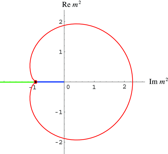
Figure 1: Curve of marginal stability in CP(1) with twisted mass. We set $4\Lambda^{2}\to 1$.

When comparing $m$ and $m_{D}$ on the opposite edges of the cut we observe monodromy around infinity,

$$(m,\,m_{D})\to(-m,\,-m_{D}-m)\,.$$ (9.4)

Correspondingly,

$$(q,\,T)\to(-q+T,\,-T)\,.$$ (9.5)

For the BPS state its mass is just $|\langle Z\rangle_{q,T}|$, and the question is which integers $q$ and $T$ correspond to physical stable states at a given value of the parameter $m^{2}$. Let us start with the range of large mass, $|m^{2}/4\Lambda^{2}|\gg 1$. In this range we are at weak coupling (quasiclassical domain) where the theory at hand has a rich spectrum of BPS states. Namely, we have light “elementary states” with $T=0$ and $q=\pm 1$ and heavy solitons with topological number $T=\pm 1$ and arbitrary integer value of $q$. Each soliton comes with an infinite tower of stable BPS states corresponding to all possible values of $q$, similar to dyons in SYM.

On the other hand, at $|m^{2}/4\Lambda^{2}|\ll 1$ we are at strong coupling. It is well known [20, 10] that in this domain the only BPS states that survive in the spectrum are

$$\{T=1,\,\,q=0\}\quad{\rm and}\quad\{T=-1,\,\,q=1\}$$

(together with their antiparticles, of course). One of these states becomes massless at $m^{2}=-4\Lambda^{2}$, more precisely, the $\{T=1,\,\,q=0\}$ soliton on the upper side of the cut, and $\{T=-1,\,\,q=1\}$ on the lower side. Thus, there is only one singular point $m^{2}=-4\Lambda^{2}$ in the $m^{2}$-plane. This is different from SU(2) SYM where there are two singular points, $u=\pm\Lambda^{2}$.

Restructuring of the BPS spectrum proves that the weak coupling domain must be separated from strong coupling by a curve of marginal stability. That the CMS exists was shown in [10], where it was not explicitly found, however. We close this gap here.

The CMS is determined by the condition that the “electric,” $q\,m$, and “magnetic,” $Tm_{D}$ parts of the exact central charge (9.1) have the same phases. This is a very simple condition,

$${\rm Re}\,\left\{\log\frac{1+\sqrt{1+4\Lambda^{2}/m^{2}}}{1-\sqrt{1+4\Lambda^{2}/m^{2}}}-2\sqrt{1+4\Lambda^{2}/m^{2}}\right\}=0\,.$$ (9.6)

The numeric solution to this equation is presented in Fig. 1 where $m^{2}$ is measured in units of $4\Lambda^{2}$.

The interval

$${\rm Im}\,m^{2}=0,\quad{\rm Re}\,m^{2}\in[-1,0]\,$$ (9.7)

represents an analytic solution of Eq. (9.6). However, this interval cannot be reached without crossing the CMS (in fact, it is a part of the cut). If we start, say, at large positive $m^{2}$ and travel towards small $m^{2}$ along the real axis, at $m^{2}\approx 2.31$ we hit a point where the elementary state $\{T=0,\,\,q=1\}$ becomes a marginally bound state of two fundamental solitons $\{T=1,\,\,q=0\}$ and $\{T=-1,\,\,q=1\}$. At slightly larger $m$ these solitons are bound, at smaller $m$ attraction changes to repulsion, and all towers of states disappear (see [19] for a detailed discussion).

As was mentioned in the beginning of this section there is a direct correspondence between CP(1) in 2D and 4D ${\cal N}=2$ SQCD with SU(2) gauge group and two flavors. The number of variables is, of course, larger in SQCD: besides the moduluar parameter $u$ we have two mass parameters, $m_{1}$ and $m_{2}$. The correspondence with CP(1) takes place at $u=m_{1}^{2}=m_{2}^{2}$ which is the root of baryonic Higgs branch [10]. The massive BPS states in 2D and 4D theories are in one-to-one correspondence upon identification $q=n_{e}$ and $T=n_{m}$.

This correspondence is more general. Thus, 2D CP($N\!-\!1$) corresponds to SU($N$) SQCD with $N$ flavors in 4D [10]. For a generic number of flavors $N_{f}\geq N$ in 4D there is also a 2D counterpart: a U(1)_G gauge theory with $N$ chiral fields with charge $+1$ and $N_{f}-N$ chiral fields with charge $-1$ and twisted masses [17]. Moreover, extending the 4D gauge group to SU($N)\times$U(1) allows one to eliminate the constraint on the matter mass parameters (e.g. for SU(2)$\times$U(1) one can consider $m_{1}^{2}\neq m_{2}^{2}$) [21, 22]. The latter is particularly instructive: the 2D theory emerges from the 4D one as a low-energy effective theory on the world sheet of the non-Abelian string (flux tube) which is a BPS soliton in the 4D theory.

An interesting question related to the 2D – 4D correspondence is what kind of theory one gets at the point of singularity which in CP(1) is $m^{2}=-4\Lambda^{2}$. From the 4D point of view at $u=m_{1}^{2}=m_{2}^{2}=-4\Lambda^{2}$ the quark and monopole vacua coalesce, a phenomenon known as the Argyres–Douglas point [23] where a nontrivial conformal field theory arises. One might suspect that the corresponding 2D theory is also nontrivially conformal. However, arguments based on the mirror representation indicate against this hypothesis [24].

10 Conclusions

In four-dimensional super-Yang–Mills theory Ferrara and Zumino were the first to point out [25] that the axial current, supercurrent and the energy-momentum tensor belonged to a supermultiplet described by a hypercurrent superfield. The superconservation of the hypercurrent is associated with the superconformal invariance of the classical theory. At the quantum level this invariance is broken by anomalies which also form a supermultiplet [11]. Much later it was realized [6] that the anomaly supermultiplet contains also the central charge anomaly.

Two-dimensional CP$(N\!-\!1)$ models are known to be cousins of four-dimensional super-Yang–Mills, which exhibit, in a simplified environment, almost all interesting phenomena typical of non-Abelian gauge theories in four dimensions, such as asymptotic freedom, instantons, spontaneous breaking of chiral symmetry, etc. [4, 26]. In spite of the close parallel existing between non-Abelian gauge theories in four dimensions and two-dimensional CP$(N\!-\!1)$ models the issue of the anomaly supermultiplet and hypercurrent equation in the twisted mass CP$(N\!-\!1)$ models has never been addressed in full. Some aspects were analyzed and important fragments reported in the literature [4, 10, 5] but, to the best of our knowledge, the full solution was not presented.

We constructed the hypercurrent superfield and the superfield of all anomalies, including that in the central charge. Thus, this question is closed.

As a byproduct, we found the curve of marginal stability in CP(1) in explicit form.

Appendix

In this Appendix we collect formulae related to the canonical quantization of the CP(1) model.

We use the fields $\phi$, $\phi^{\dagger}$, and $\psi$ as canonical coordinates, then the Lagrangian (8.2) defines the conjugated momenta,

$$\pi_{\phi}=G\partial_{t}\phi^{\dagger}+\Gamma\pi_{\psi}\psi\,,\qquad\pi_{\phi^{\dagger}}=G\partial_{t}\phi\,,\qquad\pi_{\psi}=iG\bar{\psi}\gamma^{0}\,.$$ (A.1)

Note the asymmetry between $\phi$ and $\phi^{\dagger}$, and also between $\psi$ and $\bar{\psi}$. The canonical commutation relations determine the equal-time commutators for the fields (and their time derivatives),

$$\begin{split}&\big{[}\partial_{t}\phi^{\dagger}(t,z),\phi(t,z^{\prime})\big{]}=-iG^{-1}\delta(z-z^{\prime})\,,\qquad\big{[}\partial_{t}\phi^{\dagger}(t,z),\psi(t,z^{\prime})\big{]}=iG^{-1}\Gamma\psi\,\delta(z-z^{\prime})\,,\\[5.69054pt] &\big{[}\partial_{t}\phi(t,z),\phi^{\dagger}(t,z^{\prime})\big{]}=-iG^{-1}\delta(z-z^{\prime})\,,\qquad\big{[}\partial_{t}\phi(t,z),\bar{\psi}(t,z^{\prime})\big{]}=-iG^{-1}\bar{\Gamma}\,\bar{\psi}\,\delta(z-z^{\prime})\,,\\[5.69054pt] &\big{[}\partial_{t}\phi(t,z),\partial_{t}\phi^{\dagger}(t,z^{\prime})\big{]}=-iG^{-1}\big{[}\Gamma\partial_{t}\phi-\bar{\Gamma}\partial_{t}\phi^{\dagger}+iR\,\bar{\psi}\gamma^{0}\psi\big{]}\delta(z-z^{\prime})\,,\\[5.69054pt] &\big{\{}\psi_{\alpha}(t,z),\bar{\psi}_{\beta}(t,z^{\prime})\big{\}}=G^{-1}(\gamma^{0})_{\alpha\beta}\delta(z-z^{\prime})\,.\end{split}$$ (A.2)

All other (anti)commutators vanish.

Using the expression (3.9) for the supercharges we can verify then that the canonical commutators reproduce the SUSY transformations,

$$\begin{split}&[\phi\,,\bar{Q}_{\beta}]=0\,,\qquad[\phi^{\dagger},\bar{Q}_{\beta}]=i\sqrt{2}\,\bar{\psi}_{\beta}\,,\qquad\{\psi_{\alpha}\,,\bar{Q}_{\beta}\}=\sqrt{2}\,(\hbox to0.0pt{\kern 0.53093pt/\hss}\partial-i\mu^{\dagger})_{\alpha\beta}\phi\,,\\[5.69054pt] &\{\bar{\psi}_{\alpha}\,,\bar{Q}_{\beta}\}=\sqrt{2}\,\bar{F}\,(\gamma^{0})_{\alpha\beta}\,,\qquad[\phi\,,Q_{\beta}]=i\sqrt{2}\,\psi_{\beta}\,,\qquad[\phi^{\dagger},Q_{\beta}]=0\,,\\[5.69054pt] &\{\psi_{\alpha}\,,Q_{\beta}\}=\sqrt{2}\,F\,(\gamma^{0})_{\alpha\beta}\,,\qquad\{Q_{\beta},\bar{\psi}_{\alpha}\}=\sqrt{2}\,(\hbox to0.0pt{\kern 0.53093pt/\hss}\partial+i\mu^{\dagger})_{\beta\alpha}\phi\,.\end{split}$$ (A.3)

Here

$$F=\frac{i}{2}\,\Gamma\psi\gamma^{0}\psi\,,\qquad\bar{F}=F^{\dagger}$$ (A.4)

are the upper components of superfields $\Phi$ and $\Phi^{\dagger}$.

Note that from Eq. (A.3) it follows that

$$\{G\psi_{\alpha}\,,Q_{\beta}\}=0\,,\qquad\{G\bar{\psi}_{\alpha}\,,\bar{Q}_{\beta}\}=0\,.$$ (A.5)

We used these relations to determine the anticommutators of the the currents and supercharges.

References

• [1] E. Witten and D. I. Olive, Phys. Lett. B 78, 97 (1978).
• [2] N. Seiberg and E. Witten, Nucl. Phys. B426, 19 (1994), (E) B430, 485 (1994) [hep-th/9407087].
• [3] N. Seiberg and E. Witten, Nucl. Phys. B431, 484 (1994) [hep-th/9408099].
• [4] E. Witten, Nucl. Phys. B 149, 285 (1979).
• [5] A. Losev and M. Shifman, Phys. Rev. D 68, 045006 (2003) [hep-th/0304003].
• [6] G. R. Dvali and M. A. Shifman, Phys. Lett. B 396, 64 (1997), (E) Phys. Lett. B 407, 452 (1997) [hep-th/9612128].
• [7] A. Rebhan, P. van Nieuwenhuizen and R. Wimmer, Phys. Lett. B 594, 234 (2004) [hep-th/0401116]; Quantum mass and central charge of supersymmetric monopoles: Anomalies, current renormalization, and surface terms, hep-th/0601029.
• [8] A. Rebhan, P. van Nieuwenhuizen and R. Wimmer, Nucl. Phys. B 648, 174 (2003) [hep-th/0207051].
• [9] L. Alvarez-Gaumé and D. Z. Freedman, Commun. Math. Phys.  91, 87 (1983); S. J. Gates, Nucl. Phys. B 238, 349 (1984); S. J. Gates, C. M. Hull and M. Roček, Nucl. Phys. B 248, 157 (1984).
• [10] N. Dorey, JHEP 9811, 005 (1998) [hep-th/9806056].
• [11] M. Grisaru, Anomalies in Supersymmetric Theories, in Recent Developments in Gravitation, Eds. M. Levy and S. Deser (Plenum Publishing, 1979), p. 577; for an updated version of the article see The Many Faces of the Superworld, Ed. M. Shifman (World Scientific, 2000), p. 370. For a review see M. Shifman and A. Vainshtein, Instantons Versus Supersymmetry: Fifteen Years Later, hep-th/9902018.
• [12] K. Shizuya, Phys. Rev. D 69, 065021 (2004) [hep-th/0310198].
• [13] J. Wess and J. Bagger, Supersymmetry and Supergravity, second edition, Princeton University Press, 1992.
• [14] S. Helgason, Differential geometry, Lie groups and symmetric spaces, Academic Press, New York, 1978.
• [15] A. Hanany and K. Hori, Nucl. Phys. B 513, 119 (1998) [hep-th/9707192].
• [16] M. Shifman, Supersymmetric Solitons and Topology, in Topology and Geometry in Physics, Eds. E. Bick and F.D. Steffen (Springer-Verlag, Berlin, 2005), p. 237.
• [17] N. Dorey, T. J. Hollowood and D. Tong, JHEP 9905, 006 (1999)
[hep-th/9902134].
• [18] M. A. Shifman, A. I. Vainshtein and M. B. Voloshin, Phys. Rev. D 59, 045016 (1999) [hep-th/9810068].
• [19] A. Ritz, M. A. Shifman, A. I. Vainshtein and M. B. Voloshin, Phys. Rev. D 63, 065018 (2001) [hep-th/0006028].
• [20] A. Zamolodchikov and Al. Zamolodchikov, Ann. Phys. 120 (1979) 253; Nucl. Phys. B 379 (1992) 602.
• [21] M. Shifman and A. Yung, Phys. Rev. D 70, 045004 (2004) [hep-th/0403149].
• [22] A. Hanany and D. Tong, JHEP 0404, 066 (2004) [hep-th/0403158].
• [23] P. C. Argyres and M. R. Douglas, Nucl. Phys. B 448, 93 (1995)
[hep-th/9505062].
• [24] D. Tong, private communication; A. Yung, private communication.
• [25] S. Ferrara and B. Zumino, Nucl. Phys. B 87, 207 (1975).
• [26] V. A. Novikov, M. A. Shifman, A. I. Vainshtein and V. I. Zakharov, Phys. Rept. 116, 103 (1984).