Abstract

We study an inhomogeneous decay of an unstable D-brane in the context of Dirac-Born-Infeld (DBI)-type effective action. We consider tachyon and electromagnetic fields with dependence of time and one spatial coordinate, and an exact solution is found under an exponentially decreasing tachyon potential, $e^{-|T|/\sqrt{2}}$, which is valid for the description of the late time behavior of an unstable D-brane. Though the obtained solution contains both time and spatial dependence, the corresponding momentum density vanishes over the entire spacetime region. The solution is governed by two parameters. One adjusts the distribution of energy density in the inhomogeneous direction, and the other interpolates between the homogeneous rolling tachyon and static configuration. As time evolves, the energy of the unstable D-brane is converted into the electric flux and tachyon matter.

1 Introduction

Time dependent process in string theory has been intensely studied in recent years. Assuming that an unstable D-brane decays homogeneously, the whole decay processes, in the vanishing string coupling limit $g_{s}\to 0$, can be described by the marginally deformed boundary conformal field theory (BCFT) [1]. The main results of this time dependent solution, referred as rolling tachyon, indicate that, according to time evolution, the energy density remains constant but the pressure goes to zero asymptotically.

On the other hand, spatial inhomogeneity has been another important issue. In particular, much works has been studied on tachyon solitons, such as tachyon kinks [2, 3, 4, 5, 6] and vortices [2, 7]. These solitons are interpreted as the lower dimensional D-branes on the worldvolume of the original unstable system. Thus in order to see the dynamical formation of the lower dimensional D-branes, it is indispensable to take into account the spatial inhomogeneity in the decay process of an unstable system.

The rolling of tachyon, which is inhomogeneous along one spatial direction, was considered in BCFT [8, 9, 10]. The late time behavior of the resulting energy-momentum tensor is qualitatively different from the case of the homogeneous rolling tachyon. The relevant components of the energy-momentum tensor exhibit singularities at spatially periodic locations within a finite critical time. These spatial singularities were interpreted as the codimension-one D-branes [8, 9, 10]. This subject was also considered in the boundary string field theory [11] or the DBI-type effective field theory [12, 13, 14, 15, 16, 17, 18, 19, 20, 21]. The Ref. [12] showed that the inhomogeneous solutions with a runaway tachyon potential formed caustics with multi-valued regions beyond a finite critical time, and proposed that in the presence of caustics, the higher derivatives of the tachyon field blow up. For this reason the DBI-type effective action is not reliable after the formation of caustics, since it was proposed as an effective action for the tachyon field in string theory where the higher derivatives of the tachyon field are truncated [22].

Another interesting aspect in the decay process is the dynamics at the bottom of the tachyon potential. This process has two kinds of decay products, which carry the effective degrees of freedom of the original unstable D-brane, such as energy-momentum and fundamental string charge [23]. They are called tachyon matter [1, 24] and string fluid [25]. In the tachyon vacuum, the dynamics of the system is characterized as the two degrees of freedom [26, 16, 27]. The main purpose of this paper is to explore the formation of these final states in terms of the inhomogeneous tachyon and electromagnetic fields at late time.

Let us consider the DBI-type tachyon effective action with gauge field interactions [22] described by

$$S=\int d^{p+1}x{\cal L}=-{\cal T}_{p}\int d^{p+1}x\,V(T)\sqrt{-X},$$ (1.1)

with

$$X \equiv \det X_{\mu\nu}=\det(\eta_{\mu\nu}+\partial_{\mu}T\partial_{\nu}T+F_{\mu\nu}),$$ (1.2)

$$F_{\mu\nu} = \partial_{\mu}A_{\nu}-\partial_{\nu}A_{\mu},\quad(\mu,\nu=0,1,\cdots,p),$$

where $A_{\mu}$ is an U(1) gauge field, $V(T)$ is a runaway tachyon potential, and ${\cal T}_{p}$ the tension of an unstable D$p$-brane. This action (1.1) is expected to provide a good description of an unstable D-brane in the case that the tachyon field $T$ is large, and the higher derivatives of $T$ are small. As we have seen in the rolling tachyon solution [1], the tachyon field $T$ goes to infinity at late time of the D-brane decay process. Thus DBI-type effective action describes well the late time behaviors of the process. However, once we take into account the inhomogeneity of the tachyon field without gauge field interactions, as mentioned before, DBI-type effective action becomes inadequate in a finite critical time in describing the dynamics of an unstable D-brane [12, 13, 14, 15, 17, 18, 20]. Though we include the constant electromagnetic fields, the singularity we encounter seems unavoidable [10].

In this paper, we suggest that the roles of the spacetime dependent electromagnetic fields are nontrivial on unstable D-brane system. We assume that the tachyon and electromagnetic fields depend on time and one spatial coordinate under an exponentially decreasing tachyon potential, $e^{-|T|/\sqrt{2}}$. We find an exact solution in a frame which gives vanishing momentum density provided by an appropriate electromagnetic fields. The solution represents periodic profile along the spatial direction and it involves the interesting and inaccessible regions alternatively. In the interesting regions, the solution has no singularities in time direction, and describes the late time behaviors of an unstable D-brane decay.

In section 2, we describe the calculation of the exact solution for the tachyon and electromagnetic fields. In section 3, we analyze the late time behaviors of an unstable D-brane. Section 4 is devoted to conclusion.

2 An Exact Inhomogeneous Solution

Our purpose in this work is to understand the late time behaviors of the inhomogeneous tachyon condensation in terms of an exact solution. We take a specific frame which gives the vanishing momentum density over all space-time.

Equations of motion of the tachyon $T$ and gauge field $A_{\mu}$ in the action (1.1) are written as

$$\partial_{\mu}\left(\gamma\;C^{\mu\nu}_{\rm S}\;\partial_{\nu}T\right)+{\cal T}_{p}\sqrt{-X}\;\frac{dV}{dT}=0,$$ (2.3)

$$\partial_{\mu}\left(\gamma\;C^{\mu\nu}_{\rm A}\right)=0,\qquad(\mu,\,\nu=0,1,2,\cdots p),$$ (2.4)

where $C^{\mu\nu}_{\rm S}$ and $C^{\mu\nu}_{\rm A}$ are the symmetric and anti-symmetric parts of the cofactor $C^{\mu\nu}$ of the matrix $(X)_{\mu\nu}$ in Eq. (1.2), and we define

$$\gamma\equiv\frac{{\cal T}_{p}V}{\sqrt{-X}}.$$ (2.5)

Conservation of energy-momentum is described by

$$\partial_{\mu}T^{\mu\nu}=\partial_{\mu}\left(\gamma\;C^{\mu\nu}_{\rm S}\right)=0,$$ (2.6)

where $T^{\mu\nu}$ is the energy-momentum tensor. Hamiltonian density ${\cal H}$ is expressed as

$${\cal H} = \Pi_{T}\dot{T}+\Pi^{i}\dot{A}_{i}-{\cal L}$$ (2.7)

$$= \sqrt{\Pi^{i}\Pi^{i}+\Pi_{T}^{2}+P_{i}P_{i}+(\Pi^{i}\partial_{i}T)^{2}+{\cal T}_{p}^{2}V^{2}\det(h)}-A_{0}\partial_{i}\Pi^{i},$$

where $\dot{T}\equiv\partial_{0}T$, $h_{ij}=\delta_{ij}+\partial_{i}T\partial_{j}T+F_{ij}$, ($i,j=1,2,\cdots p$), the conjugate momenta, $\Pi_{T}$ and $\Pi^{i}$, for the tachyon $T$ and gauge field $A_{i}$ respectively, and the conserved linear momentum, $P_{i}$, associated with the translation symmetry are

$$\Pi^{i} \equiv \frac{\delta S}{\delta\dot{A}_{i}}=\gamma C_{{\rm A}}^{ti},$$

$$\Pi_{T} \equiv \frac{\delta S}{\delta\dot{T}}=\gamma C_{{\rm S}}^{t\mu}\partial_{\mu}T,$$

$$P_{i} = \Pi^{j}F_{ji}-\Pi_{T}\partial_{i}T.$$ (2.8)

From now on, let us introduce an exponentially decreasing tachyon potential,

$$V(T)=V_{0}\,e^{-T/R},$$ (2.9)

where $V_{0}$ and $R$ are arbitrary constants. We consider an ansatz for fields which live on the worldvolume of the unstable D$p$-brane,

$$T=T(x^{0},x^{1}),\quad E\equiv F_{02}(x^{0},x^{1}),\quad B\equiv F_{12}(x^{0},x^{1}),$$ (2.10)

and, for simplicity, turn off all other components of the gauge fields.

Then the only non-vanishing linear momentum in Eq. (2.8) is

$$P_{1} = -\gamma\left(\dot{T}T^{\prime}+EB\right),$$ (2.11)

where $T^{\prime}=\partial_{1}T$. Here, we choose the zero-momentum frame due to cancelation of the effects of tachyon and electromagnetic fields,

$$EB=-\dot{T}T^{\prime}.$$ (2.12)

Additionally the determinant $X$ in Eq. (1.2) under condition (2.12) is factored as

$$-X=(1+T^{\prime 2}+B^{2})(1-\dot{T}^{2}-E^{2}).$$ (2.13)

Conservation of energy-momentum, $\partial_{\mu}T^{\mu\nu}=0$, under the condition (2.12) leads to an observation that the energy density $T^{00}$ has only spatial dependence and $T^{11}$ time dependence, i.e.,

$$T^{00} = T^{00}(x)={\cal T}_{p}V\sqrt{\frac{1+{T^{\prime}}^{2}+B^{2}}{1-\dot{T}^{2}-E^{2}}}\,,$$ (2.14)

$$T^{11} = T^{11}(t)=-{\cal T}_{p}V\sqrt{\frac{1-\dot{T}^{2}-E^{2}}{1+{T^{\prime}}^{2}+B^{2}}}\,,$$ (2.15)

where we used the notations, $t=x^{0}$ and $x=x^{1}$. The Eqs. (2.14) and (2.15) are rewritten by

$${\cal T}_{p}V(T)=f(t)g(x),$$ (2.16)

$$\frac{1-\dot{T}^{2}-E^{2}}{1+{T^{\prime}}^{2}+B^{2}}=\left(\frac{f(t)}{g(x)}\right)^{2},$$ (2.17)

where

$$f(t)\equiv\sqrt{-T^{11}(t)},\qquad g(x)\equiv\sqrt{T^{00}(x)}.$$ (2.18)

Under the tachyon potential (2.9), the equation of motion for the tachyon field (2.3) is simplified as

$$\frac{\ddot{T}}{1-\dot{T}^{2}-E^{2}}-\frac{T^{\prime\prime}}{1+T^{\prime 2}+B^{2}}-\frac{1}{R}=0.$$ (2.19)

Using the Eqs. (2.16), (2.17), and (2.19), we arrive at the following important results,

$$E=E(t),\qquad B=B(x).$$ (2.20)

The derivation of this equation is rather technical and therefore is recorded in Appendix. The factorization (2.16) implies

$$\dot{T}(t)=-\frac{R\dot{f}(t)}{f(t)},\qquad T^{\prime}(x)=-\frac{Rg^{\prime}(x)}{g(x)}.$$ (2.21)

From the relations (2.12), (2.20), and (2.21) we get

$$E(t) = \alpha\dot{T}=-\frac{\alpha R\dot{f}}{f},$$

$$B(x) = -\frac{1}{\alpha}T^{\prime}=\frac{Rg^{\prime}}{\alpha g},$$ (2.22)

where $\alpha$ is an arbitrary constant. Inserting the expressions (2.21) and (2.22) into the Eq. (2.17), we obtain the first-order differential equations for $f(t)$ and $g(x)$,

$$\dot{f}^{2}-\frac{f^{2}}{R^{2}(1+\alpha^{2})}+\frac{f^{4}}{\xi R^{2}(1+\alpha^{2})}=0,$$ (2.23)

$$g^{\prime 2}+\frac{\alpha^{2}g^{2}}{R^{2}(1+\alpha^{2})}-\frac{\alpha^{2}g^{4}}{\xi R^{2}(1+\alpha^{2})}=0,$$ (2.24)

where $\xi$ is a positive constant. Solutions for the equations (2.23) – (2.24) are given by

$$f(t) = \pm\sqrt{\xi}\,{\rm sech}\left(\frac{t-c_{1}}{R\sqrt{1+\alpha^{2}}}\right),$$ (2.25)

$$g(x) = \pm\sqrt{\xi}\,{\rm sec}\left(\frac{\alpha(x-c_{2})}{R\sqrt{1+\alpha^{2}}}\right),$$ (2.26)

where $c_{1}$ and $c_{2}$ are integration constants, which represent the translation symmetries along time and spatial directions respectively. Of course, the expressions (2.23) – (2.26) satisfy the $2$-component of the gauge equation (2.4),

$$g^{2}\dot{E}=f^{2}B^{\prime}.$$ (2.27)

Substituting the solution (2.25) into the Eq. (2.5), we find

$$\gamma=\frac{{\cal T}_{p}V}{\sqrt{-X}}=\frac{{\cal T}_{p}V}{\sqrt{(1+T^{\prime 2}+B^{2})(1-\dot{T}^{2}-E^{2})}}=\xi.$$

Finally we obtain an exact solution for the tachyon field by inserting the expression (2.25) into (2.16),

$$T(t,x)=R\ln\left[\frac{{\cal T}_{p}V_{0}}{\gamma}\,{\rm cosh}\left(\frac{t-c_{1}}{R\sqrt{1+\alpha^{2}}}\right)\left|{\rm cos}\left(\frac{\alpha(x-c_{2})}{R\sqrt{1+\alpha^{2}}}\right)\right|\right].$$ (2.28)

This solution is characterized by two parameters, $\gamma$ and $\alpha$. We will investigate the roles of these parameters in section 3. At first glance this result seems to be unnatural since $T(t,x)$ has the periodic divergencies in the limit $\left|\cos\left(\frac{\alpha(x-c_{2})}{R\sqrt{1+\alpha^{2}}}\right)\right|\to 0$ due to the property of cosine function. Actually in the spatially periodic regions at the initial time $t=0$ which satisfy

$$\left|\cos\left(\frac{\alpha(x-c_{2})}{R\sqrt{1+\alpha^{2}}}\right)\right|<\frac{(\gamma/{\cal T}_{p}V_{0})}{\cosh\left(\frac{c_{1}}{R\sqrt{1+\alpha^{2}}}\right)}<1,$$ (2.29)

the corresponding tachyon field $T(t=0,x)$ is negative. In these regions the DBI-type effective action does not provide a good description for the dynamics of an unstable D-brane as we explained in the section 1. In order to describe the late time behaviors of the decay process of an unstable D-brane, we restrict our interest to the spatially periodic regions which correspond to the large positive value of tachyon field. We will describe the details in the next section.

3 Late Time Behaviors of the Decay Process

It was observed in the previous section that there is an exact solution (2.28) for the exponentially decreasing tachyon potential in momentum zero frame. Our purpose in this section is to analyze the solution (2.28) in superstring theory. Since a total charge is conserved (we will mention later in detail at subsection 3.3) and the tachyon potential has ${\rm Z}_{2}$-symmetry under $T\to-T$, and runaway property $V(\pm\infty)=0$, we employ a tachyon potential composed of two parts,

$$V(T)=V_{0}\,e^{-\frac{|T|}{\sqrt{2}}}=\left\{\begin{array}[]{lclcc}V_{0}\,e^{-\frac{T}{\sqrt{2}}}&{}\hfil&T>0&{}\hfil&({\rm I})\\ V_{0}\,e^{\frac{T}{\sqrt{2}}}&{}\hfil&T<0&{}\hfil&({\rm II})\end{array}\right..$$ (3.32)

Tachyon profile is read from the Eq. (2.28) in the regions (I) and (II) by choosing the appropriate integration constants, $c_{1}$ and $c_{2}$,

$$T(t,x)=\left\{\begin{array}[]{lcc}\sqrt{2}\ln\left[\frac{{\cal T}_{p}V_{0}}{\gamma}\,{\rm cosh}\left(\frac{t+t_{0}}{\sqrt{2}\sqrt{1+\alpha^{2}}}\right)\cos\left(\frac{\alpha x_{\rm I}}{\sqrt{2}\sqrt{1+\alpha^{2}}}-\frac{\pi}{2}\right)\right],&{}\hfil&({\rm I})\\ -\sqrt{2}\ln\left[\frac{{\cal T}_{p}V_{0}}{\gamma}\,{\rm cosh}\left(\frac{t+t_{0}}{\sqrt{2}\sqrt{1+\alpha^{2}}}\right)\cos\left(\frac{\alpha x_{{\rm II}}}{\sqrt{2}\sqrt{1+\alpha^{2}}}+\frac{\pi}{2}\right)\right],&{}\hfil&({\rm II})\end{array}\right.,$$ (3.35)

where $x_{\rm I}$($x_{{\rm II}}$) represents the spatial coordinate belonging to the region (I)((II)), $t_{0}$ is some large value introduced to figure out the late time behaviors of the inhomogeneous fields. The ranges of $x_{\rm I}$ and $x_{{\rm II}}$ are given by

$$x^{-}_{4m+1}\leq x_{\rm I}\leq x^{+}_{4m+1},$$

$$\tilde{x}^{-}_{4m+1}\leq x_{{\rm II}}\leq\tilde{x}^{+}_{4m+1},\quad(m=\mbox{integer}).$$ (3.36)

where $x^{\pm}_{4m+1}$ and $\tilde{x}^{\pm}_{4m+1}$ denote

$$x^{\pm}_{4m+1} = \frac{\sqrt{2}\sqrt{1+\alpha^{2}}}{\alpha}\left[\pm\cos^{-1}\left(\frac{\gamma}{{\cal T}_{p}V_{0}}\right)+\frac{(4m+1)\pi}{2}\right],$$

$$\tilde{x}^{\pm}_{4m+1} = \frac{\sqrt{2}\sqrt{1+\alpha^{2}}}{\alpha}\left[\pm\cos^{-1}\left(\frac{\gamma}{{\cal T}_{p}V_{0}}\right)-\frac{(4m+1)\pi}{2}\right],\quad(0\leq\gamma\leq{\cal T}_{p}V_{0}).$$ (3.37)

There are periodic regions, where the decay process of the unstable D-brane is not described well by the solution (3.35), referred as inaccessible regions,

$$\tilde{x}^{+}_{4m+1}<x_{{\rm inaccessible}}<x^{-}_{4m+1},\quad\mbox{and}\quad x^{-}_{4m+1}<x_{{\rm inaccessible}}<\tilde{x}^{+}_{4m+5}.$$ (3.38)

To illustrate the solution (3.35) graphically, we draw two figures for the tachyon potential $V(T)$ and tachyon field $T(t,x)$ in Fig.1. The arrows in Fig.1 (b) represent growing tachyon field as time elapses. The corresponding tachyon fields spans the ranges at initial time $t=0$,

$$T_{0}\leq T_{{\rm I}}(t,x)\leq T_{{\rm max}},\qquad-T_{{\rm max}}\leq T_{{\rm II}}(t,x)\leq-T_{0},$$ (3.39)

where

$$T_{0}=\sqrt{2}\ln\cosh\left(\frac{t_{0}}{\sqrt{2}\sqrt{1+\alpha^{2}}}\right),$$

$$T_{{\rm max}}=\sqrt{2}\ln\left[\frac{{\cal T}_{p}V_{0}}{\gamma}\,{\rm cosh}\left(\frac{t_{0}}{\sqrt{2}\sqrt{1+\alpha^{2}}}\right)\right].$$

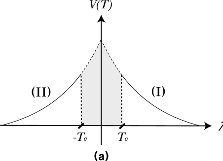
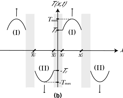
Figure 1: (a) Shape of $V(T)=e^{\frac{-|T|}{\sqrt{2}}}$ for $|T|\geq T_{0}$. (b) Profiles of tachyon field $T(x,t)$. Shaded regions represent the inaccessible regions.

Electromagnetic fields in Eq. (2.22) take the functional forms

$$E(t) = \alpha\dot{T}(t)=\left\{\begin{array}[]{lcc}\frac{\alpha}{\sqrt{1+\alpha^{2}}}\tanh\left(\frac{t+t_{0}}{\sqrt{2}\sqrt{1+\alpha^{2}}}\right),&{}\hfil&({\rm I})\\ -\frac{\alpha}{\sqrt{1+\alpha^{2}}}\tanh\left(\frac{t+t_{0}}{\sqrt{2}\sqrt{1+\alpha^{2}}}\right),&{}\hfil&({\rm II})\end{array}\right.,$$ (3.42)

$$B(x) = -\frac{1}{\alpha}T^{\prime}(x)=\left\{\begin{array}[]{lcc}\frac{1}{\sqrt{1+\alpha^{2}}}\tan\left(\frac{\alpha x_{\rm I}}{\sqrt{2}\sqrt{1+\alpha^{2}}}-\frac{\pi}{2}\right),&{}\hfil&({\rm I})\\ -\frac{1}{\sqrt{1+\alpha^{2}}}\tan\left(\frac{\alpha x_{{\rm II}}}{\sqrt{2}\sqrt{1+\alpha^{2}}}+\frac{\pi}{2}\right),&{}\hfil&({\rm II})\end{array}\right..$$ (3.45)

The configuration for the tachyon field (3.35) represents the time evolution of the spatially periodic profiles governed by two parameters, $\gamma$ and $\alpha$. $\gamma$ adjusts the distribution of the energy density, while $\alpha$ is the scaling parameter of time and controls the period. We investigate the roles of the parameter $\alpha$.

3.1 $\alpha\to 0$ case : Homogeneous rolling tachyon

When $\alpha$ goes to zero, the period of tachyon profile approaches infinity. Thus the corresponding solution in Eq. (3.35) describes the homogeneous rolling tachyon, i.e., the spatial inhomogeneity is neglected. In the region (I) for $m=0$ in Eq. (3), the Eqs. (3.35), (3.42), and (3.45) are given by

$$T(t,x) = \sqrt{2}\ln\left[\frac{{\cal T}_{p}V_{0}}{\gamma}\cosh\left(\frac{t+t_{0}}{\sqrt{2}}\right)\cos\left(\frac{\alpha x_{\rm I}}{\sqrt{2}}\right)\right],$$

$$B(x) = \tan\left(\frac{\alpha x_{\rm I}}{\sqrt{2}}\right),$$

$$\dot{T}(t) = \tanh\left(\frac{t+t_{0}}{\sqrt{2}}\right),$$

$$T^{\prime}(x) = E(t)=0$$ (3.46)

with

$$-\sqrt{2}\cos^{-1}\left(\frac{{\cal T}_{p}V_{0}}{\gamma}\right)\leq\alpha x_{\rm I}\leq\sqrt{2}\cos^{-1}\left(\frac{{\cal T}_{p}V_{0}}{\gamma}\right).$$

This analysis is also applicable to the case of the region (II). It is well-known that when the tachyon and electromagnetic fields in the DBI-type effective action (1.1) depend on only one spacetime coordinate, the results of equations of motion for the given system show that all the electromagnetic fields are constants [5, 28]. In this limit, the period of magnetic field $B(x)$ reaches to infinity but its amplitude remains finite. Therefore the results in Eqs. (3.46) represent a homogeneous rolling tachyon with almost constant magnetic field and constant energy density $T^{00}={\cal T}_{p}^{2}V_{0}^{2}/\gamma$.

The pressure and tachyon matter density are

$$T^{11}(t)=T^{22}=-\gamma\,{\rm sech}^{2}\left(\frac{t+t_{0}}{\sqrt{2}\sqrt{1+\alpha^{2}}}\right),$$

$$\Pi_{T}(t,x)=\frac{{\cal T}_{p}^{2}}{\gamma}\tanh\left(\frac{t+t_{0}}{\sqrt{2}}\right).$$ (3.47)

In the limit of $t\to\infty$, we obtain the pressureless matter with constant energy density and tachyon matter density [24].

3.2 $\alpha\to\infty$ case : Static configurations

On the other hand, when $\alpha$ goes to infinity, $x^{\pm}_{4m+1}$ and $\tilde{x}^{\pm}_{4m+1}$ reach to fixed finite values,

$$x^{\pm}_{4m+1} = \sqrt{2}\left[\pm\cos^{-1}\left(\frac{\gamma}{{\cal T}_{p}V_{0}}\right)+\frac{(4m+1)\pi}{2}\right],$$

$$\tilde{x}^{\pm}_{4m+1} = \sqrt{2}\left[\pm\cos^{-1}\left(\frac{\gamma}{{\cal T}_{p}V_{0}}\right)-\frac{(4m+1)\pi}{2}\right].$$ (3.48)

From the Eq. (3.35) we can easily check that the time dependence disappears and the configuration of tachyon becomes a static solution in this limit. The expressions of the Eqs. (3.35), (3.42), and (3.45) at finite time $t<<\alpha$ in the region (I) are given by

$$T(t,x) = \ln\left[\frac{{\cal T}_{p}V_{0}}{\gamma}\cos\left(\frac{x_{\rm I}}{\sqrt{2}}-\frac{\pi}{2}\right)\right],$$

$$T^{\prime}(x) = -\tan\left(\frac{x_{\rm I}}{\sqrt{2}}-\frac{\pi}{2}\right),$$

$$E(t) = \dot{T}(t)=B(x)=0,$$ (3.49)

where $\gamma$ adjusts the distribution of energy density for the given static configuration. In the limit $\gamma\to 0$, most of energy is localized at $x^{\pm}_{4m+1}$. The energy stored in half period of one cycle in the limit is obtained by

$$\left(\int_{-x_{0}}^{\tilde{x}^{+}_{1}}dx+\int_{x^{-}_{1}}^{x_{0}}dx\right)\,T^{00}(x)|_{\gamma\to 0}=2\sqrt{2}\,{\cal T}_{p}V_{0},$$ (3.50)

where $x_{0}=\sqrt{1+\alpha^{2}}\pi/\sqrt{2}\alpha$. Since our exact solution is valid only for large $T$, the decent relation (3.50) is approximately correct.

As we have worked in the above subsections 3.1 and 3.2, $\alpha$ is the only parameter which governs the time scale and period along spatial direction for a given $\gamma$ in the solution (3.35). Thus $\alpha$ is an interpolating parameter between the homogeneous rolling tachyon ($\alpha=0$) and the static configuration ($\alpha\to\infty$).

3.3 Late time behaviors

As time elapses, the tachyon profiles (3.35) in the regions (I) and (II) grow up along the arrows in Fig.1 (b). In the interesting regions (3), all physical quantities can be expressed explicitly, and the unstable system evolves without singularity in our system. Non-vanishing components of energy-momentum tensor are given by

$$T^{00}(x) = \left\{\begin{array}[]{lcc}\gamma\sec^{2}\left(\frac{\alpha x_{\rm I}}{\sqrt{2}\sqrt{1+\alpha^{2}}}-\frac{\pi}{2}\right),&{}\hfil&({\rm I})\\ \gamma\sec^{2}\left(\frac{\alpha x_{{\rm II}}}{\sqrt{2}\sqrt{1+\alpha^{2}}}+\frac{\pi}{2}\right),&{}\hfil&({\rm II})\end{array}\right.,$$ (3.53)

$$T^{11}(t) = -\gamma\,{\rm sech}^{2}\left(\frac{t+t_{0}}{\sqrt{2}\sqrt{1+\alpha^{2}}}\right)\,\,{\rm for}\,\,({\rm I})\,\,{\rm and}\,\,({\rm II}),$$ (3.54)

$$T^{22}(t,x) = \left\{\begin{array}[]{lcc}-\gamma\left[1-\frac{1}{1+\alpha^{2}}\tanh^{2}\left(\frac{t+t_{0}}{\sqrt{2}\sqrt{1+\alpha^{2}}}\right)+\frac{\alpha^{2}}{1+\alpha^{2}}\tan^{2}\left(\frac{\alpha x_{\rm I}}{\sqrt{2}\sqrt{1+\alpha^{2}}}-\frac{\pi}{2}\right)\right],&{}\hfil&({\rm I})\\ -\gamma\left[1-\frac{1}{1+\alpha^{2}}\tanh^{2}\left(\frac{t+t0}{\sqrt{2}\sqrt{1+\alpha^{2}}}\right)+\frac{\alpha^{2}}{1+\alpha^{2}}\tan^{2}\left(\frac{\alpha x_{{\rm II}}}{\sqrt{2}\sqrt{1+\alpha^{2}}}+\frac{\pi}{2}\right)\right],&{}\hfil&({\rm II})\end{array}\right..$$ (3.57)

Since the momentum density flow is zero in the interesting regions of the solution (3), the initial energy density distribution is not changed in time direction. As time goes to infinity, pressure along the inhomogeneous direction, $x$, goes to zero exponentially [24]. $T^{22}$ component depends on $t$ and $x$-coordinates for finite $\alpha$. However, in $\alpha\to 0$ limit (homogeneous rolling tachyon limit), $T^{22}$ and $T^{11}$ share with the same behavior in time direction.

The solution (3.35) also provides the expression for the electric flux density which satisfies Gauss constraint $\partial_{i}\Pi^{i}=0$ and the gauge equation (2.27),

$$\Pi_{2} = \alpha\Pi_{T}=\left\{\begin{array}[]{lc}\frac{\alpha\gamma}{\sqrt{1+\alpha^{2}}}\tanh\left(\frac{t+t_{0}}{\sqrt{2}\sqrt{1+\alpha^{2}}}\right)\sec^{2}\left(\frac{\alpha x_{\rm I}}{\sqrt{2}\sqrt{1+\alpha^{2}}}-\frac{\pi}{2}\right),&({\rm I})\\ -\frac{\alpha\gamma}{\sqrt{1+\alpha^{2}}}\tanh\left(\frac{t+t_{0}}{\sqrt{2}\sqrt{1+\alpha^{2}}}\right)\sec^{2}\left(\frac{\alpha x_{{\rm II}}}{\sqrt{2}\sqrt{1+\alpha^{2}}}+\frac{\pi}{2}\right),&({\rm II})\end{array}\right..$$ (3.61)

This expression denotes that absolute values of the electric flux and tachyon matter densities increase in the D-brane decay process. However, total string charge accumulated in the interesting regions is conserved in one period ;

$$\left(\int_{\tilde{x}^{-}_{4m+1}}^{\tilde{x}^{+}_{4m+1}}dx+\int_{x^{-}_{4m+1}}^{x^{+}_{4m+1}}dx\right)\,\Pi_{2}(t,x)=0.$$ (3.62)

Combining the Eqs. (3.42), (3.53), and (3.61), we obtain the following two relations,

$$1-\dot{T}^{2}-E^{2}={\rm sech}^{2}\left(\frac{t+t_{0}}{\sqrt{2}\sqrt{1+\alpha^{2}}}\right),$$ (3.63)

$$\Pi_{2}^{2}+\Pi_{T}^{2}={\cal H}^{2}\tanh^{2}\left(\frac{t+t_{0}}{\sqrt{2}\sqrt{1+\alpha^{2}}}\right),$$ (3.64)

where the Hamiltonian density ${\cal H}$ is given by

$${\cal H}=\sqrt{\Pi_{2}^{2}+\Pi_{T}^{2}+{\cal T}_{p}^{2}V^{2}(1+T^{\prime 2}+B^{2})}=T^{00}(x).$$ (3.65)

Since there is no singularity in interesting regions in time direction, the obtained solution describes safely the decay processes near the tachyon vacuum ($V\to 0$) in $t\to\infty$ limit. As time goes to infinity, the time dependent electric fields in the regions (I) and (II) become constants with opposite sign,

$$E(t)|_{T\to\infty}=\alpha\dot{T}(t)|_{T\to\infty}=\left\{\begin{array}[]{lcc}\frac{\alpha}{\sqrt{1+\alpha^{2}}},&{}\hfil&({\rm I})\\ -\frac{\alpha}{\sqrt{1+\alpha^{2}}},&{}\hfil&({\rm II})\end{array}\right..$$ (3.68)

These relations in tachyon vacuum ($V\to 0$) reproduce the well-known expression [29, 26],

$$1-\dot{T}^{2}-E^{2}\to 0.$$ (3.69)

This result leads to an intriguing observation. As we have discussed in subsection 3.2, the system gives a static configuration in the limit $\alpha\to\infty$. At initial time the electric field is equal to zero in Eq. (3.49). As time evolves to infinity ($t/\alpha\to\infty$), the electric field becomes critical and $\dot{T}$ is suppressed to zero,

$$|E(t)|\to 1,\qquad|\dot{T}(t)|\to 0.$$ (3.70)

As we have seen in Eq. (3.65), the energy density is composed of three parts, such as string flux density ($\Pi_{2}$), tachyon matter density ($\Pi_{T}$), and tachyon potential energy. As time evolves, the contributions from $\Pi_{2}$ and $\Pi_{T}$ increase, while the contribution from the tachyon potential decreases. Finally the unstable D-brane disappears at the tachyon vacuum ($V\to 0$). The resultant energy density in the tachyon vacuum is composed of two parts [25, 26],

$${\cal H}^{2}=\Pi_{2}^{2}+\Pi_{T}^{2},$$ (3.71)

where

$$\Pi_{2}(t,x)|_{T\to\infty}=\alpha\Pi_{T}(t,x)|_{T\to\infty}=\left\{\begin{array}[]{lc}\frac{\alpha\gamma}{\sqrt{1+\alpha^{2}}}\sec^{2}\left(\frac{\alpha x_{\rm I}}{\sqrt{2}\sqrt{1+\alpha^{2}}}-\frac{\pi}{2}\right),&({\rm I})\\ -\frac{\alpha\gamma}{\sqrt{1+\alpha^{2}}}\sec^{2}\left(\frac{\alpha x_{{\rm II}}}{\sqrt{2}\sqrt{1+\alpha^{2}}}+\frac{\pi}{2}\right),&({\rm II})\end{array}\right..$$ (3.74)

4 Conclusion

We have investigated the spatially inhomogeneous decay of an unstable D-brane in DBI-type effective action. We found an exact solution under an exponentially decreasing tachyon potential. The resulting solution involves the periodic inaccessible region along the inhomogeneous direction, while the behavior in time direction is well-defined. The solution is governed by two parameters, $\gamma$ and $\alpha$. $\gamma$ adjusts the distribution of energy density, and $\alpha$ is an interpolating parameter between the homogeneous rolling tachyon and the static solution.

It is well-known that the inhomogeneous rolling tachyon with a runaway type tachyon potential forms caustics with multi-valued regions beyond a finite critical time. After the critical time the unstable system may not be described by DBI-type tachyon effective action. However, as we have seen in section 3, it was possible to describe the late time behaviors of an unstable D-brane in the interesting regions due to the nontrivial roles of the spacetime dependent electromagnetic fields. Therefore our solution may open a possibility to find the caustic free tachyon field solution in a specific setting with spacetime dependent electromagnetic fields in tachyon effective field theory.

As time evolves, all physical quantities are well defined and go to tachyon vacuum ($V=0$) without developing further singularities in the interesting regions. Electric flux density, which is proportional to the tachyon matter density with a constant ratio $\alpha$, increase in magnitude, but have the opposite signs in the region (I) and (II). They finally reach to space dependent finite configurations. As a result, the energy stored in the unstable D-brane at the initial stage is converted to that of the string fluid and the tachyon matter. Since two interesting regions in one cycle (See Fig.1 (b)) go to the different vacua ($T\to\infty$ and $T\to-\infty$) in $t\to\infty$ limit, inaccessible region between them contains a topological kink which seems to be interpreted as D$(p-1)\bar{\rm D}(p-1)$ or D$(p-1){\rm F}1\bar{\rm D}(p-1){\rm F}1$ .

Appendix: Derivation of $E=E(t)$ and $B=B(x)$

In this appendix we present detailed derivation of $E(t)$ and $B(x)$. From the Eqs. (2.16), (2.17), and (2.19), we obtain

$$E^{2} = 1-\dot{T}^{2}-R\ddot{T}+Rf^{2}\,\rho(x),$$

$$B^{2} = -\left(1+T^{\prime 2}+RT^{\prime\prime}\right)+Rg^{2}\,\sigma(t),$$ (A.1)

where

$$\rho(x)\equiv\frac{T^{\prime\prime}}{g^{2}},\qquad\sigma(t)\equiv\frac{\ddot{T}}{f^{2}}.$$ (A.2)

Differentiations of the two equations in Eq. (A.1) with respect to $x$ and $t$ yield

$$2EE^{\prime} = Rf^{2}\,\rho^{\prime}(x),$$

$$2B\dot{B} = Rg^{2}\,\dot{\sigma}(t).$$ (A.3)

Product of the two equations in Eq. (A.3) gives

$$E^{\prime 2}=\dot{B}^{2}=-\frac{f^{3}g^{3}}{4\dot{f}g^{\prime}}\rho^{\prime}\dot{\sigma},$$ (A.4)

where we used the Eqs. (2.12), (2.21), and Bianchi identity for the gauge field strength,

$$E^{\prime}=\dot{B}.$$ (A.5)

The relations in Eqs. (A.3) and (A.4) imply that $E$, $B$, $E^{\prime}$, and $\dot{B}$ are separable functions of $t$ and $x$. The separable properties for the electromagnetic fields, $E$ and $B$, in Eq. (A.1) impose on the conditions for the functions, $f(t)$ and $g(x)$,

$$1-\dot{T}^{2}-R\ddot{T}=cf^{2},\,$$

$$1+T^{\prime 2}+RT^{\prime\prime}=dg^{2},$$ (A.6)

where $c$ and $d$ are arbitrary constants. Insertion of the relations (A.6) into the Eq. (A.1) produces

$$E^{2}B^{2}=f^{2}g^{2}(c+R\rho(x))(-d+R\sigma(t))=\frac{R^{4}\dot{f}^{2}g^{\prime 2}}{f^{2}g^{2}}=\dot{T}^{2}T^{\prime 2}.$$ (A.7)

The Eq. (A.7) is separated into two parts,

$$R\ddot{T} = \frac{\dot{T}^{2}}{\zeta}+df^{2},$$

$$RT^{\prime\prime} = \zeta T^{\prime 2}-cg^{2},$$ (A.8)

where $\zeta$ is an arbitrary positive constant. The relations between Eqs. (A.6) and (Appendix: Derivation of $E=E(t)$ and $B=B(x)$) give

$$\left(1+\frac{1}{\zeta}\right)\dot{T}^{2}+(c+d)f^{2}-1=0,$$

$$(1+\zeta)T^{\prime 2}-(c+d)g^{2}+1=0.$$ (A.9)

Differentiating the relations in Eq. (Appendix: Derivation of $E=E(t)$ and $B=B(x)$), we find

$$\sigma(t) = \frac{\ddot{T}}{f^{2}}=\frac{\zeta(c+d)}{R(1+\zeta)}=\mbox{constant},$$

$$\rho(x) = \frac{T^{\prime\prime}}{g^{2}}=-\frac{c+d}{R(1+\zeta)}=\mbox{constant}.$$ (A.10)

Using the Eqs. (A.1) and (Appendix: Derivation of $E=E(t)$ and $B=B(x)$), we finally obtain

$$E=E(t),\qquad B=B(x).$$ (A.11)

References

• [1] A. Sen, “Rolling tachyon,” JHEP 0204, 048 (2002) [arXiv:hep-th/0203211] ; A. Sen, “Tachyon matter,” JHEP 0207, 065 (2002) [arXiv:hep-th/0203265].
• [2] A. Sen, “Dirac-Born-Infeld action on the tachyon kink and vortex,” Phys. Rev. D 68, 066008 (2003) [arXiv:hep-th/0303057].
• [3] N. Lambert, H. Liu and J. Maldacena, “Closed strings from decaying D-branes,” arXiv:hep-th/0303139.
• [4] P. Brax, J. Mourad and D. A. Steer, “Tachyon kinks on non BPS D-branes,” Phys. Lett. B 575, 115 (2003) [arXiv:hep-th/0304197] ; E. J. Copeland, P. M. Saffin and D. A. Steer, “Singular tachyon kinks from regular profiles,” Phys. Rev. D 68, 065013 (2003) [arXiv:hep-th/0306294] ; D. Bazeia, R. Menezes and J. G. Ramos, “Regular and periodic tachyon kinks,” Mod. Phys. Lett. A 20, 467 (2005) [arXiv:hep-th/0401195].
• [5] C. Kim, Y. Kim and C. O. Lee, “Tachyon kinks,” JHEP 0305, 020 (2003) [arXiv:hep-th/0304180] ; C. Kim, Y. Kim, O-K. Kwon and C. O. Lee, “Tachyon kinks on unstable Dp-branes,” JHEP 0311, 034 (2003) [arXiv:hep-th/0305092].
• [6] C. Kim, Y. Kim, O-K. Kwon and H. U. Yee, “Tachyon Kinks in Boundary String Field Theory,” arXiv:hep-th/0601206.
• [7] Y. Kim, B. Kyae and J. Lee, “Global and local D-vortices,” JHEP 0510, 002 (2005) [arXiv:hep-th/0508027]; I. Cho, Y. Kim and B. Kyae, “DF-strings from D3 D3-bar as cosmic strings,” arXiv:hep-th/0510218.
• [8] A. Sen, “Time evolution in open string theory,” JHEP 0210, 003 (2002) [arXiv:hep-th/0207105].
• [9] F. Larsen, A. Naqvi and S. Terashima, “Rolling tachyons and decaying branes,” JHEP 0302, 039 (2003) [arXiv:hep-th/0212248].
• [10] S. J. Rey and S. Sugimoto, “Rolling of modulated tachyon with gauge flux and emergent fundamental string,” Phys. Rev. D 68, 026003 (2003) [arXiv:hep-th/0303133].
• [11] A. Ishida and S. Uehara, “Rolling down to D-brane and tachyon matter,” JHEP 0302, 050 (2003) [arXiv:hep-th/0301179].
• [12] G. N. Felder, L. Kofman and A. Starobinsky, “Caustics in tachyon matter and other Born-Infeld scalars,” JHEP 0209, 026 (2002) [arXiv:hep-th/0208019].
• [13] S. Mukohyama, “Inhomogeneous tachyon decay, light-cone structure and D-brane network problem in tachyon cosmology,” Phys. Rev. D 66, 123512 (2002) [arXiv:hep-th/0208094].
• [14] M. Berkooz, B. Craps, D. Kutasov and G. Rajesh, “Comments on cosmological singularities in string theory,” JHEP 0303, 031 (2003) [arXiv:hep-th/0212215].
• [15] J. M. Cline and H. Firouzjahi, “Real-time D-brane condensation,” Phys. Lett. B 564, 255 (2003) [arXiv:hep-th/0301101].
• [16] O-K. Kwon and P. Yi, “String fluid, tachyon matter, and domain walls,” JHEP 0309, 003 (2003) [arXiv:hep-th/0305229].
• [17] G. N. Felder and L. Kofman, “Inhomogeneous fragmentation of the rolling tachyon,” Phys. Rev. D 70, 046004 (2004) [arXiv:hep-th/0403073].
• [18] N. Barnaby, “Caustic formation in tachyon effective field theories,” JHEP 0407, 025 (2004) [arXiv:hep-th/0406120].
• [19] K. L. Panigrahi, “D-brane dynamics in Dp-brane background,” Phys. Lett. B 601, 64 (2004) [arXiv:hep-th/0407134].
• [20] O. Saremi, L. Kofman and A. W. Peet, “Folding branes,” Phys. Rev. D 71, 126004 (2005) [arXiv:hep-th/0409092].
• [21] F. Canfora, “A note on tachyon dynamics,” Phys. Lett. B 625, 277 (2005) [arXiv:gr-qc/0508082].
• [22] M. R. Garousi, “Tachyon couplings on non-BPS D-branes and Dirac-Born-Infeld action,” Nucl. Phys. B 584, 284 (2000) [arXiv:hep-th/0003122]; E. A. Bergshoeff, M. de Roo, T. C. de Wit, E. Eyras and S. Panda, “T-duality and actions for non-BPS D-branes,” JHEP 0005, 009 (2000) [arXiv:hep-th/0003221]; J. Kluson, “Proposal for non-BPS D-brane action,” Phys. Rev. D 62, 126003 (2000) [arXiv:hep-th/0004106].
• [23] P. Yi, “Membranes from five-branes and fundamental strings from Dp branes,” Nucl. Phys. B 550, 214 (1999) [arXiv:hep-th/9901159].
• [24] A. Sen, “Field theory of tachyon matter,” Mod. Phys. Lett. A 17, 1797 (2002) [arXiv:hep-th/0204143].
• [25] G. W. Gibbons, K. Hori and P. Yi, “String fluid from unstable D-branes,” Nucl. Phys. B 596, 136 (2001) [arXiv:hep-th/0009061].
• [26] G. Gibbons, K. Hashimoto and P. Yi, “Tachyon condensates, Carrollian contraction of Lorentz group, and fundamental strings,” JHEP 0209, 061 (2002) [arXiv:hep-th/0209034].
• [27] H. U. Yee and P. Yi, “Open / closed duality, unstable D-branes, and coarse-grained closed Nucl. Phys. B 686, 31 (2004) [arXiv:hep-th/0402027].
• [28] C. Kim, H. B. Kim, Y. Kim and O-K. Kwon, “Electromagnetic string fluid in rolling tachyon,” JHEP 0303, 008 (2003) [arXiv:hep-th/0301076].
• [29] P. Mukhopadhyay and A. Sen, “Decay of unstable D-branes with electric field,” JHEP 0211, 047 (2002) [arXiv:hep-th/0208142].