Exact time dependent Hopf solitons in $3+1$ dimensions

Abstract

We construct an infinite number of exact time dependent soliton solutions, carrying non-trivial Hopf topological charges, in a $3+1$ dimensional Lorentz invariant theory with target space $S^{2}$. The construction is based on an ansatz which explores the invariance of the model under the conformal group $SO(4,2)$ and the infinite dimensional group of area preserving diffeomorphisms of $S^{2}$. The model is a rare example of an integrable theory in four dimensions, and the solitons may play a role in the low energy limit of gauge theories.

Introduction - Solitons have a very important role in several areas of Physics. In particular, they are useful in the understanding of many non-perturbative (strong coupling) phenomena. The appearance of solitons requires a rich symmetry structure, leading to conservation laws, and therefore they underlie the integrability properties of the models. Although the $1+1$ soliton theory is well developed, very few exact results are known about solitons in higher dimensions afsg . In this Letter we construct an infinite number of exact soliton solutions, carrying Hopf topological charges, in a $3+1$ dimensional, Lorentz invariant theory, and possesing an infinite number of conservation laws. An important feature of the solitons is that, in the far past and far future, their energy density is vanishingly small and distributed over a large region of space. For finite times the energy density builds up in a small portion of space. In addition, the solutions depend upon a free parameter that allows to re-scale their size and rate of time evolution. The condition for the total energy to be conserved also implies that the Hopf topological charge should be non-trivial. The model is a rare and interesting example of an integrable theory in four dimensions, and its solitons may have an important role in the low energy limit of the Yang-Mills theories, as we discuss at the end of this Letter. In addition, our work may be of interest in the study of the solitons of the Skyrme-Faddeev model fn . The theory is defined by the action

$$S=-\frac{1}{e^{2}}\int d^{4}x\,H_{\mu\nu}^{2}$$ (1)

where $H_{\mu\nu}$ is the pull-back of the area form on $S^{2}$

$$H_{\mu\nu}\equiv-2i\frac{\left(\partial_{\mu}u\partial_{\nu}u^{*}-\partial_{\nu}u\partial_{\mu}u^{*}\right)}{\left(1+\mid u\mid^{2}\right)^{2}}={\vec{n}}\cdot\left(\partial_{\mu}{\vec{n}}\wedge\partial_{\nu}{\vec{n}}\right)$$ (2)

with $u$ being a complex scalar field, related to the triplet of scalar fields ${\vec{n}}$ living on $S^{2}$ (${\vec{n}}^{2}=1$) through the stereographic projection ${\vec{n}}=\left(u+u^{*},-i\left(u-u^{*}\right),\mid u\mid^{2}-1\right)/\left(1+\mid u\mid^{2}\right)$. The Euler-Lagrange equations are

$$\partial_{\mu}{\cal K}^{\mu}=0\;;\qquad\qquad{\cal K}_{\mu}\equiv H_{\mu\nu}\,\partial^{\nu}u$$ (3)

together with its complex conjugate. The action (1) and the eqs. of motion (3) are invariant under the conformal group $SO(4,2)$ of four-dimensional Minkowski space-time babelon . They are also invariant under the area preserving diffeomorphisms of $S^{2}$, and the infinite set of associated Noether currents are given by razumov

$$J_{\mu}^{G}=\left(\delta G/\delta u\right){\cal K}_{\mu}+\left(\delta G/\delta u^{*}\right){\cal K}_{\mu}^{*}$$ (4)

where $G$ is any functional of $u$ and $u^{*}$, but not of their derivatives.

Solutions - We introduce the coordinates

$$x^{0} = \left(a/p\right)\,\sin\zeta\;;\quad\;\;\,x^{1}=\left(a/p\right)\,\cos\varphi/\sqrt{1+y}$$ (5)

$$x^{3} = \left(a/p\right)\sin\xi\sqrt{y/\left(1+y\right)};\;\,x^{2}=\left(a/p\right)\sin\varphi/\sqrt{1+y}$$

with $p=\cos\zeta-\cos\xi\,\sqrt{y/(1+y)}$, and $a$ is a constant with dimension of length. The range of the coordinates are: $y\geq 0$, $0\leq\xi\,,\,\varphi\leq 2\pi$, and $0\leq\zeta\leq\pi$. Notice that the range of $\zeta$ is restricted because $\left(\zeta,y,\xi,\varphi\right)$ and $\left(\zeta+\pi,y,\xi+\pi,\varphi+\pi\right)$ give the same point on Minkowski space-time. We introduce the ansatz afz99 ; babelon

$$u=\sqrt{\left(1-g\right)/g}\;\;e^{i\left(m_{1}\,\xi+m_{2}\,\varphi+m_{3}\,\zeta\right)}$$ (6)

with $g=g\left(y\right)$, and $0\leq g\leq 1$. In order for $u$ to be single valued we need $m_{1}$ and $m_{2}$ to be integers. In addition, $\left(\zeta=0,y,\xi,\varphi\right)$ and $\left(\zeta=\pi,y,\xi+\pi,\varphi+\pi\right)$ correspond to the same point $\left(x^{0}=0,x^{1},x^{2},x^{3}\right)$. Therefore, we also need $m_{1}+m_{2}+m_{3}=2N$, with $N$ being an integer, in order for $u$ to be single valued. Replacing (6) into (3) we reduce those four-dimensional non-linear partial differential equations into a single linear ordinary differential equation given by

$$\partial_{y}\left(\Lambda\,\partial_{y}g\right)=0\;;\quad\Lambda\equiv m_{1}^{2}\,\left(1+y\right)+m_{2}^{2}\,y\left(1+y\right)-m_{3}^{2}\,y$$ (7)

The analysis of the solutions is very simple. For $m_{2}=0$ the solution is logarithmic and so diverges for $y\rightarrow\infty$. Since we need $0\leq g\leq 1$, for $y\geq 0$, the only acceptable solution is $g={\rm constant}$, which we shall discard. For the same reasons $\Lambda$ can not have real and positive zeroes for $m_{2}\neq 0$. Since those are given by $y_{\pm}=-b\pm\sqrt{\Delta}$, with

$$b = \left[\left(m_{1}+m_{3}\right)\left(m_{1}-m_{3}\right)+m_{2}^{2}\right]/2m_{2}^{2}$$ (8)

$$\Delta = \left[\left(m_{1}+m_{3}\right)^{2}-m_{2}^{2}\right]\left[\left(m_{1}-m_{3}\right)^{2}-m_{2}^{2}\right]/4m_{2}^{4}$$

we can not have $b<0$ and $\Delta\geq 0$, which happen whenever $\left(m_{1}+m_{3}\right)/m_{2}\geq 1$ and $\left(m_{1}-m_{3}\right)/m_{2}\leq-1$ or $\left(m_{1}-m_{3}\right)/m_{2}\geq 1$ and $\left(m_{1}+m_{3}\right)/m_{2}\leq-1$. Therefore, the solutions satisfying the boundary conditions $g\left(0\right)=1$ and $g\left(\infty\right)=0$, are ($m_{2}\neq 0$)

$$g = \frac{b}{y+b}\;;\qquad{\rm for}\;\;\Delta=0\;;\;\;\;b>0$$ (9)

$$g = \frac{{\rm ArcTan}\left(\sqrt{-\Delta}/\left(y+b\right)\right)}{{\rm ArcTan}\left(\sqrt{-\Delta}/b\right)}\;;\quad{\rm for}\;\;\Delta<0\;;\;\;\;{\rm any}\;\;b$$

$$g = \frac{\ln\left[\left(y+b+\sqrt{\Delta}\right)/\left(y+b-\sqrt{\Delta}\right)\right]}{\ln\left[\left(b+\sqrt{\Delta}\right)/\left(b-\sqrt{\Delta}\right)\right]}\;;\;\;{\rm for}\;\;\Delta,b>0$$

They are all monotonically decreasing functions of $y$, from $1$ at $y=0$, to $0$ for $y\rightarrow\infty$.

In order to visualize the time evolution of the solutions we have to take slices of constant $x^{0}=c\,t$. The best way to do it, is to trade the coordinate $\zeta$ in favour of the dimensionless time $\tau=ct/a$. From (5) one has that $\tau^{2}p^{2}=1-\cos^{2}\zeta$, which is a quadratic equation for $\cos\zeta$ in terms of $\tau^{2}$. The two solutions lead to equivalent descriptions of the constant time slices. With one of those choices, the Cartesian space coordinates on the time slices are written as

$$x^{1}=\frac{a}{q}\,\cos\varphi\;;\quad x^{2}=\frac{a}{q}\,\sin\varphi\;;\quad x^{3}=\frac{a}{q}\,\sin\xi\,\sqrt{y}$$ (10)

with $q=\frac{\sqrt{1+y+\tau^{2}\left(1+y\sin^{2}\xi\right)}-\cos\xi\sqrt{y}}{1+\tau^{2}}$. The form of the solutions can be understood through their surfaces of constant $n_{3}$, the third component of the scalar fields on $S^{2}$ (see (2) and below). From (6) one has that $n_{3}=1-2g$ . So, fixed $n_{3}$ means fixed $g$, which in its turn means fixed $y$, since from (9), we have that $g$ is a monotonic function of $y$. Therefore, for a given fixed time $\tau$ the surfaces of constant $n_{3}$ are obtained from (10) by varying the angles $\xi$ and $\varphi$, and keeping $y$ fixed. Notice that such surfaces are valid for any solution given in (6) and (9). The only thing is that the chosen fixed value of $y$ corresponds to different values of $n_{3}$ for different solutions. From (10) and the form of $q$, we see that such surfaces are invariant under rotations around the $x_{3}$-axis, and under the time reflection $\tau\rightarrow-\tau$. They are toroidal surfaces around the $x^{3}$-axis. In Figure 1 we show their cross sections, at some fixes values of time, through the half-plane $x^{3}\rho$, with $\rho=\sqrt{x_{1}^{2}+x_{2}^{2}}$. Some general properties of the solutions are: i) The surface for $n_{3}=-1$, which implies $g=1$ and so $y=0$, is a circle on the plane $x_{3}=0$ with center at the origin and radius $a\sqrt{1+\tau^{2}}$; ii) The surface for $n_{3}=1$, which implies $g=0$ and so $y\rightarrow\infty$, corresponds to the $x_{3}$-axis plus the spatial infinity, for any time $\tau$ (The reason is that for $\xi\neq 0$, the limit $y\rightarrow\infty$ gives $\mid q\mid\rightarrow\infty$, and for $\xi=0$ gives $q\rightarrow 0$); iii) For $\tau=0$ the surfaces of constant $n_{3}$, for $-1<n_{3}<1$, are torus centered around the origin with a tickness that grows as $n_{3}$ varies from $-1$ to $1$. As $\tau$ flows towards the future or the past, those torus get ticker and their cross section deform from a circle to a quarter moon shape as shown in Figure 1; iv) The solution performs one single oscillation as $\tau$ varies from $-\infty$ to $\infty$. Although the surfaces of constant $n_{3}$ are symmetrical under the interchange $\tau\leftrightarrow-\tau$, the same is not true for the energy density as shown below; v) Due to Derrick’s scaling argument, the theory (1) can not have stable static solutions in $3+1$ dimensions, and so our solutions can not be put at rest, even though the limit of large $a$ slow down their time evolution.

Figure 1: Cross sections of the surfaces of constant $n_{3}$ for $n_{3}=1-2g\left(y=1\right)$, and at the times $\tau=ct/a=0,2,5,8$. The vertical and horizontal axis correspond to $x^{3}/a$ and $\rho/a$ respectively. The surfaces are invariant under $\tau\rightarrow-\tau$

Hopf charge - The condition for finite energy requires the field ${\vec{n}}$ to be constant at spatial infinity. For any fixed time, our solutions have ${\vec{n}}\rightarrow\left(0,0,1\right)$ for $r\rightarrow\infty$ ($r^{2}=x_{1}^{2}+x_{2}^{2}+x_{3}^{2}$). Therefore, for topological considerations, we can compactify $\leavevmode\hbox{\rm I\kern-1.79993ptR}^{3}$ into $S^{3}$, and the solution defines a Hopf map $S^{3}\rightarrow S^{2}$, for any fixed time. The Hopf index is calculated as follows: given the solution (6) and (9) we map $\leavevmode\hbox{\rm I\kern-1.79993ptR}^{3}$ into $S^{3}_{Z}$ through $Z=\left(\begin{array}[]{c}z_{1}\\ z_{2}\end{array}\right)=\left(\begin{array}[]{c}\sqrt{1-g}\,e^{i\left(m_{1}\xi+m_{3}\zeta\right)}\\ \sqrt{g}\,e^{-i\left(m_{2}\varphi\right)}\end{array}\right)$ with $Z^{\dagger}\,Z=1$, and so the four real parameters in $Z$ parametrize $S^{3}_{Z}$. Then we map $S^{3}_{Z}$ into $S^{2}_{u}$ through $u=z_{1}/z_{2}$. The Hopf index is defined as

$$Q_{H}=\frac{1}{4\pi^{2}}\,\int d^{3}x\,{\vec{A}}\cdot\left(\nabla\wedge{\vec{A}}\right)$$ (11)

with ${\vec{A}}=i\left(Z^{\dagger}{\vec{\nabla}}Z-{\vec{\nabla}}Z^{\dagger}\,Z\right)/2$. Using , one then gets ${\vec{A}}\cdot\left({\vec{\nabla}}\wedge{\vec{A}}\right)=-\frac{\partial_{y}g}{a\rho^{4}}m_{2}\left(m_{1}\left(a^{2}+R^{2}\right)+2m_{3}\,x^{0}\,x^{3}\right)$, with $R^{2}=x_{0}^{2}+x_{1}^{2}+x_{2}^{2}+x_{3}^{2}$. Notice that $y$ is an even function of all $x^{\mu}$’s [12] and so is $\partial_{y}g$. Therefore, the term proportional to $m_{3}$, being odd in $x^{3}$, vanishes when integrated on space. The volume element on the time slices (10) is

$$d^{3}x=dy\,d\xi\,d\varphi\,a\rho^{4}/\left(a^{2}+R^{2}\right)$$ (12)

The Hopf index (11) for the solutions (6) and (9) is then

$$Q_{H}=-m_{1}m_{2}\left(g\left(\infty\right)-g\left(0\right)\right)=m_{1}m_{2}$$ (13)

Noether charges - Among the charges associated to the currents (4) there is an infinite abelian subset corresponding to the cases where $G$ is a functional of the norm of $u$ only, or equivalently a functional of $g=1/(1+\mid u\mid^{2})$ (see (6)). One can easily check that the Poisson brackets of the densities $J_{0}^{G}$, associated to such choice of $G$, does vanish razumov . If one substitute (6) into (4) and uses [12] one gets that, for $G$ being a functional of $g$ only, $J_{0}^{G}=4\left(\partial_{y}g\right)^{2}\frac{\delta G}{\delta g}\left[2m_{1}\left(1+y\right)x^{0}x^{3}+m_{3}y\left(a^{2}+R^{2}\right)\right]/a\rho^{4}$. Since $y$ is an even function of all Cartesian coordinates $x^{\mu}$, it follows that the term propotional to $m_{1}$, being odd in $x^{3}$, vanishes when integrated on the whole space. Using (12) one gets that the corresponding Noether charges are $Q^{G}=16\pi^{2}m_{3}\int_{0}^{\infty}dy\,y\,\left(\partial_{y}g\right)^{2}\frac{\delta G}{\delta g}$. Using (7) and (9) one gets

$$\partial_{y}g=-\,\frac{C}{\Lambda}\;;\quad C=\left(m_{1}^{2}+m_{2}^{2}-m_{3}^{2}\right)w/\ln\frac{1+w}{1-w}$$ (14)

with $w=\sqrt{\Delta}/b$, and $\Delta$, $b$ satisfying any of the three conditions in (9). Notice that in all those cases we have $C>0$, and in particular for $\Delta=0$ one has $C=\left(m_{1}^{2}+m_{2}^{2}-m_{3}^{2}\right)/2$. Then taking $G=g^{n}/16\pi^{2}n!$, one gets that such charges evaluated on the solutions (9) are given by

$$Q^{(n)}=m_{3}\;F^{(n)}\left(w\right)\;;\qquad n=1,2,3\ldots$$ (15)

with

$$F^{(n)}\left(w\right)=\left(\ln(1+w)/(1-w)\right)^{-n-1}\left[-2\epsilon_{-}\left(n\right)\right.$$

$$+\sum_{l=1}^{n}\left.\left(\frac{\epsilon_{+}\left(n-l\right)}{w}-\epsilon_{-}\left(n-l\right)\right)\frac{1}{l!}\left(\ln\frac{1+w}{1-w}\right)^{l}\right]$$ (16)

with $\epsilon_{\pm}\left(n\right)=\left(1\pm\left(-1\right)^{n}\right)/2$. For the case $\Delta=0$, those charges simplify to $Q^{(n)}=m_{3}n/(n+2)!$. The case $n=1$ corresponds to the $U(1)$ subgroup of the $S^{2}$-area preserving diffeomorphism group generated by $u\rightarrow e^{i\alpha}u$.

Angular Momentum - The angular momentum is given by $L_{i}=\frac{1}{2}\varepsilon_{ijk}\int d^{3}xM^{0}_{(jk)}$, with $M^{\mu}_{(\rho\sigma)}=T^{\mu}_{\rho}x_{\sigma}-T^{\mu}_{\sigma}x_{\rho}$, and $T^{\mu}_{\nu}$ being the canonical energy-momentum tensor associated to (1). For the solutions (6) and (9) it is

$$L_{3}=\frac{128\pi^{2}}{e^{2}}\,m_{2}\,m_{3}\,F^{(1)}\left(w\right)\,;\qquad\;\;L_{1}=L_{2}=0$$ (17)

Energy - The Hamiltonian density associated to (1) is ${\cal H}=(2/e^{2})\left(\sum_{i}H_{0i}^{2}+\sum_{i<j}H_{ij}^{2}\right)$, with $i,j=1,2,3$. For the ansatz configurations (6) one gets that

$${\cal H}=\frac{8}{e^{2}}\left(\partial_{y}g\right)^{2}\left(m_{1}^{2}{\cal E}_{1}+m_{2}^{2}{\cal E}_{2}+m_{3}^{2}{\cal E}_{3}+2m_{1}m_{3}{\cal E}_{13}\right)$$ (18)

with ${\cal E}_{13}=\frac{4x^{0}x^{3}\left(a^{2}+R^{2}\right)}{a^{2}\rho^{6}}$, ${\cal E}_{1}=\frac{4}{\rho^{4}}\left(1+y+\frac{2x_{0}^{2}r^{2}}{a^{2}\rho^{2}}\right)$, ${\cal E}_{2}=\frac{4}{\rho^{4}}\left(y\left(1+y\right)+\frac{x_{0}^{2}\left(a^{2}+s^{2}\right)^{2}}{2a^{4}\rho^{2}}\right)$, and ${\cal E}_{3}=\frac{4}{\rho^{4}}\left(y+\frac{2x_{0}^{2}x_{3}^{2}}{a^{2}\rho^{2}}\right)$. The energy density is axially symmetric, and invariant under the joint parity transformations $x^{0}\rightarrow-x^{0}$ and $x^{3}\rightarrow-x^{3}$. In Figure 2 we show the time evolution of ${\cal H}$ for two particular solitons. Notice that it resembles the time evolution of some types of Ward’s solitons ward .

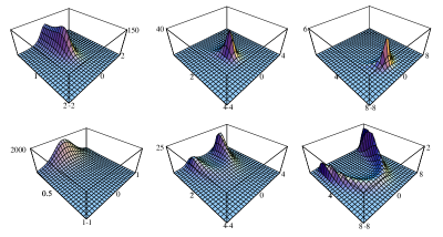
Figure 2: Plots of the energy density ${\cal H}$ (18), in units of $\frac{8}{e^{2}}$, as a function of $\rho/a$ (left-front axis) and $x^{3}/a$ (right-front axis). ${\cal H}$ is invariant under rotations around the $x^{3}$-axis and under the joint parity transformations $\tau\rightarrow-\tau$ and $x^{3}\rightarrow-x^{3}$. The top row correspond to the soliton with $\left(m_{1},m_{2},m_{3}\right)=\left(1,4,1\right)$, at the times $\tau=ct/a=0,2,6$, and the bottom row to the soliton with $\left(m_{1},m_{2},m_{3}\right)=\left(4,1,1\right)$, at the same times. These two solitons have the same total energy (19), Noether charges (15) and Hopf charge (13), but the soliton $\left(1,4,1\right)$ has four times more angular momentum (17) than the soliton $\left(4,1,1\right)$.

The total energy is only conserved when $m_{1},m_{2}\neq 0$, and so when the Hopf charge (13) is non vanishing. Indeed, the integration of the term involving ${\cal E}_{13}$ vanishes since it is odd in $x^{3}$. The other terms give $\int d^{3}x\left(\partial_{y}g\right)^{2}{\cal E}_{3}=\frac{8\pi^{2}}{a}\int_{0}^{\infty}dy\,\left(\partial_{y}g\right)^{2}\,y$, and $\int d^{3}x\left(\partial_{y}g\right)^{2}\left(m_{1}^{2}{\cal E}_{1}+m_{2}^{2}{\cal E}_{2}\right)=\frac{8\pi^{2}}{a}\left[\frac{\tau^{2}}{1+\tau^{2}}W+\int_{0}^{\infty}dy\,\left(\partial_{y}g\right)^{2}\,\left(m_{1}^{2}\,\left(1+y\right)+m_{2}^{2}\,y\left(1+y\right)\right)\right]$, with $W=\int_{0}^{\infty}dy\,\left(\partial_{y}g\right)^{2}\,\left(m_{1}^{2}-m_{2}^{2}\,y^{2}\right)$. From (14) one then gets that $W=C^{2}y/\Lambda\mid_{y=0}^{y=\infty}$. In our analysis below (8) we concluded that we have to have $m_{2}\neq 0$ for the solutions to be well behaved. But $W$ does not vanish if $m_{1}=0$ and $m_{2}\neq 0$. Therefore, in order for the total energy to be time independent we need $m_{1}\neq 0$ too. Consequently, $E=\frac{\left(8\pi\right)^{2}}{a\,e^{2}}\int_{0}^{\infty}dy\,\left(\partial_{y}g\right)^{2}\,\Omega$, with $\Omega=m_{1}^{2}\left(1+y\right)+m_{2}^{2}\,y\left(1+y\right)+m_{3}^{2}\,y=\Lambda+2m_{3}^{2}\,y$. Using (14) one gets $\int_{0}^{\infty}dy\,\left(\partial_{y}g\right)^{2}\Lambda=-C\left(g\left(\infty\right)-g\left(0\right)\right)$, and the remaining integral is proportional to $Q^{(1)}$ (see (15)). Then one gets that

$$E=\frac{\left(8\pi\right)^{2}}{a\,e^{2}}\left[C+2\,m_{3}^{2}\,F^{(1)}\right]$$ (19)

with $C$ and $F^{(1)}$ given in (14) and (16). In the case $\Delta=0$, which implies $m_{2}^{2}=\left(m_{1}\pm m_{3}\right)^{2}$ (see (8)), the energy reduces to $E=\frac{\left(8\pi\right)^{2}}{a\,e^{2}}\left(m_{1}^{2}+\frac{1}{3}m_{3}^{2}\pm m_{1}m_{3}\right)$. The energy $E$ (19) is invariant under the interchange $m_{1}\leftrightarrow m_{2}$, and under the change of sign of any integer $m_{i}$, $i=1,2,3$, individually. Therefore, it is $16$-fold degenerate for $m_{1}\neq m_{2}$, $m_{3}\neq 0$, and that is reduced by factors $2$’s according $m_{1}=m_{2}$ or $m_{3}=0$ (remember there are no physically acceptable solutions for $m_{1},m_{2}=0$). In any case, such degeneracy is completely lifted by considering the values of the Hopf charge $Q_{H}$ (13), the Noether charge $Q^{(1)}$ (15) (or any other $Q^{(n)}$), and the angular momentum $L_{3}$ (17).

The solitons we have constructed have a connection with the Yang-Mills (YM) theory. At the classical level, they correspond to vacuum configurations of YM. In fact, any solution of any field theory with target space $S^{2}$ can be mapped into a vacuum of $SU(2)$ YM. Indeed, consider a $SU(2)$ gauge theory with gauge potencial ${\vec{W}}_{\mu}$, with a Higgs field ${\vec{\phi}}$ in the triplet representation (the arrows stand for the orientation in the $SU(2)$ algebra). The Higgs vacuum, $V\left(\phi\right)=0$ and $D_{\mu}{\vec{\phi}}=0$, is achieved with ${\vec{\phi}}=v{\vec{n}}$, and ${\vec{W}}_{\mu}=\frac{1}{e}{\vec{n}}\wedge\partial_{\mu}{\vec{n}}+{\vec{n}}B_{\mu}$, where $e$ is the gauge coupling constant, ${\vec{n}}^{2}=1$, $v$ is the minimum of $V$, and $B_{\mu}$ is an arbitrary $U(1)$ gauge potential. That is in fact, the field configuration of a ’t Hooft-Polyakov monopole away from its core. The field strength is ${\vec{F}}_{\mu\nu}={\vec{n}}\left(\frac{1}{e}H_{\mu\nu}+\partial_{\mu}B_{\nu}-\partial_{\nu}B_{\mu}\right)$, with $H_{\mu\nu}$ as in (2). If we take $B_{\mu}$ to be proportional to the potential of the Hopf charge density (11), i.e. $B_{\mu}=-\frac{i}{e}\left(Z^{\dagger}\partial_{\mu}Z-\partial_{\mu}Z^{\dagger}\,Z\right)$, then $\partial_{\mu}B_{\nu}-\partial_{\nu}B_{\mu}=-\frac{1}{e}H_{\mu\nu}$, for any $Z$, and ${\vec{F}}_{\mu\nu}$ vanishes. Notice that, although ${\vec{F}}_{\mu\nu}$ is local in the fields ${\vec{n}}$, the same is not true for ${\vec{W}}_{\mu}$. The same connection can be made with a pure YM (without Higgs) using the Cho-Faddeev-Niemi decomposition of ${\vec{W}}_{\mu}$ fndecomp . Such connection with YM is independent of the dynamics of the fields ${\vec{n}}$. The theory (1) becomes relevant at the quantum level. At low energies it is reasonable to take ${\vec{n}}$ as an order parameter and so a degree of freedom of ${\vec{W}}_{\mu}$. The low energy effective action $S_{\rm eff.}$ of YM will then contain (1) as one of its terms, since it is a marginal operator gies . The classical solutions of $S_{\rm eff.}$ play an important role in the generating functional calculations, and the solutions we have constructed can then perhaps be useful in a perturbative expansion of $S_{\rm eff.}$ around (1). See dubois for a further connection between (1) and YM.

Acknowledgements: The author is grateful to J. Sanchez Guillen and W. J. Zakrzewski for helpful discussions. Work partially supported by CNPq.

References

(1)
O. Alvarez, L. A. Ferreira and J. Sanchez Guillen,
Nucl. Phys. B 529 (1998) 689
[arXiv:hep-th/9710147].
(2)
L. D. Faddeev and A. J. Niemi,
Nature 387, 58 (1997)
[arXiv:hep-th/9610193];
R. A. Battye and P. M. Sutcliffe,
Phys. Rev. Lett. 81, 4798 (1998)
[arXiv:hep-th/9808129];
J. Hietarinta, P. Salo,
Phys. Rev. D 62, 081701 (2000).
(3)
O. Babelon and L. A. Ferreira,
JHEP 0211, 020 (2002)
[arXiv:hep-th/0210154];
A.C.R. Bonfim and L.A. Ferreira, in preparation.
(4)
L. A. Ferreira and A. V. Razumov,
Lett. Math. Phys. 55, 143 (2001)
[arXiv:hep-th/0012176].
(5)
H. Aratyn, L. A. Ferreira and A. H. Zimerman,
Phys. Rev. Lett. 83, 1723 (1999)
[arXiv:hep-th/9905079]
(6) R. S. Ward,
J. Math. Phys. 29, 386 (1988).
T. A. Ioannidou and W. J. Zakrzewski,
J. Math. Phys. 39, 2693 (1998)
[arXiv:hep-th/9802122].
T. A. Ioannidou,
J. Math. Phys. 37, 3422 (1996)
[arXiv:hep-th/9604126].
(7)
L. D. Faddeev and A. J. Niemi,
Phys. Rev. Lett. 82, 1624 (1999)
[arXiv:hep-th/9807069];
Y. M. Cho,
Phys. Rev. D 21, 1080 (1980); and
Phys. Rev. D 23, 2415 (1981).
(8) H. Gies,
Phys. Rev. D 63, 125023 (2001), hep-th/0102026
(9)
M. Dubois-Violette and Y. Georgelin,
Phys. Lett. B 82, 251 (1979);
M. Dubois-Violette, Mathématique et Physique, Progress in
Mathematics, Vol. 37, Birkhäuser (1983), p. 43-64.