Dynamics of domain walls intersecting black holes

Abstract

Previous studies concerning the interaction of branes and black holes suggested that a small black hole intersecting a brane may escape via a mechanism of reconnection. Here we consider this problem by studying the interaction of a small black hole and a domain wall composed of a scalar field and simulate the evolution of this system when the black hole acquires an initial recoil velocity. We test and confirm previous results, however, unlike the cases previously studied, in the more general set-up considered here, we are able to follow the evolution of the system also during the separation, and completely illustrate how the escape of the black hole takes place.

Introduction. It is well known that primordial black holes and domain walls may have formed in the early universe: on the one hand, cosmological density perturbations may have collapsed and formed small black holes pbh1 ; pbh2 , on the other hand, during the cooling phase after the big bang, the series of phase transitions that have occurred may have produced extended topological structures like domain walls book . In view of the stringent constraints that both primordial black holes and domain walls provide, understanding how these objects interact could help in clarifying many issues regarding the early universe and, possibly, be of phenomenological relevance.

In the past few years, the interaction between black holes and domain walls has been object of some study. Of particular significance, in relation to our work, are the results of Refs. frolov1 ; dm1 ; dm2 ; dm3 ; dm4 . Ref. frolov1 considers the Dirac-Nambu-Goto approximation for the domain wall and proves the existence of a family of static wall solutions intersecting the black hole event horizon. Subsequent work extended those results to the case of thick walls, Refs. dm1 ; dm2 ; dm3 ; dm4 .

An important problem where the previous studies may find application is the scattering of a black hole and a domain wall stoj . When the domain wall moves towards the black hole, it is expected to be captured by the black hole and the static configurations mentioned above may describe this process in the adiabatic limit, namely when the relative motion is very slow. It is likely that the membrane will experience large deformations and topology changing processes will take place, but the adiabatic limit cannot easily resolve this issue. A full dynamical simulation is necessary, and it would also help to clarify what happens in more extreme situations, which are more likely to have occurred in the early universe, where the adiabatic approximation may not be adequate.

Aside from the motivations mentioned above, the exciting possibility of observing mini black holes at forthcoming collider experiments, as predicted by low scale gravity theories add ; rs ; dam ; dl ; gt , has rejuvenated interest in the subject. In such models our universe has a domain wall structure, the brane, that is embedded in a higher dimensional space; the standard model particles are confined on the brane and gravity propagates throughout the higher dimensional bulk spacetime. Many realizations of this scenario result in lowering the Planck scale to a few TeV and share the common prediction that a small black hole forms when two particles collide at sufficiently high energy with small impact parameter. Once the black hole is produced, it will emit Hawking radiation, and this can in principle be observed at the CERN LHC or in cosmic ray facilities. The radiation of the black hole will partly go into lower dimensional fields, localised on the brane, and partly into higher dimensional modes, which will cause the black hole to recoil into the extra dimensions.

The recoil of the black hole in the context described above was first studied in Ref. frolov within a toy model consisting of two scalar fields, one describing the black hole and the other a possible quanta emitted by the black hole in the process of evaporation; the coupling between them is fixed as to reproduce the probability of emission of a scalar quanta from the black hole as prescribed by the Hawking formula, and a delta function potential is used to mimic the interaction between the black hole and the brane. In the approximation that the interaction with the brane is negligibly small, it is shown that, as soon as a quanta is emitted in the extra dimension, the black hole will slide off the brane. Although this has the important observable effect of a sudden interruption of the radiation on the brane (Ref. stojkovic explores some possible phenomenological consequences), it is not clear how the separation process occurs. To clarify this issue and to have further evidence for the conclusions of Ref. frolov , two of the present authors have considered the interaction between ‘mini’ black holes and branes from the different perspective of studying the dynamics of branes in black hole spacetimes, Ref.flachi . Specifically, by treating the brane in the Dirac-Nambu-Goto approximation, we have shown that, once the black hole acquires an initial recoil velocity perpendicularly to the brane, an instability develops and the brane tends to envelop the black hole. This suggests a mechanism of escape for the black hole due to the reconnection of the brane. In some approximation the time of escape can be estimated and it was found to be shorter than the evaporation time. This fact may have important phenomenological consequences.

The previous claim certainly deserves reconsideration and one of our motivations is to test the robustness of the conclusions of Ref. flachi by modeling the brane as a domain wall composed of a scalar field. Also, unlike the Dirac-Nambu-Goto case previously studied, modeling the brane as a domain wall allows one to describe reconnection phenomena. In our case, this means that we can follow the evolution of the system while the separation of the black hole occurs, and completely illustrate how the escape takes place.

Domain wall dynamics. The system we intend to study consists of a domain wall intersecting a black hole. As customary, we consider black holes whose mass $m$ exceeds the fundamental Planck scale $M$, in order to make quantum gravity corrections negligible. Also, the size of the mini black hole is assumed to be smaller than the characteristic length of the extra dimensions. We shall restrict our analysis to the case when the wall tension is small enough, as this allows us to ignore the self-gravity of the wall. In this regime, the mini black hole is completely immersed in the higher dimensional spacetime and can be adequately described by asymptotically flat solutions tangherlini ; mp

$$ds^{2}=-f(r)dt^{2}+f^{-1}(r)dr^{2}+r^{2}d\Omega_{d-2}^{2}~{},$$ (1)

where $d\Omega_{d-2}$ is the line element of a $(d-2)-$dimensional unit sphere,

$$f(r)=1-\left({r_{H}\over r}\right)^{d-3}$$

and $r_{H}$ is the horizon radius. We use units in which $c=\hbar=1$.

Since the character of vacuum structures is generally insensitive to the details of the model, we limit ourselves to a scalar effective field theory with quartic potential

$$V(\Phi)={\lambda\over 4}(\Phi^{2}-\eta^{2})^{2}~{}.$$ (2)

The domain wall solutions of this model in flat space have tension $\sigma\simeq\sqrt{\lambda}\eta^{3}$ and thickness ${\tt t}\simeq 1/\sqrt{\lambda}\eta$. The coupling constant $\lambda$ is of order $\Lambda^{4-d}$, with $\Lambda\lesssim M$ being the cutoff of the effective field theory. We can neglect the quantum corrections to the domain wall-type configurations at weak coupling $\Lambda^{(d-2)/2}\gg\eta$. This implies $\sigma\gg{\tt t}^{1-d}$, and hence we have $\sigma r_{H}^{d-2}/M\gg(r_{H}/{\tt t})^{d-1}(M_{d}/M)^{(d-2)/(d-3)}$, where we introduced the $d$-dimensional Planck mass $M_{d}=G^{1/(d-2)}$. Requirement of negligible self-gravity therefore implies that the wall is not very thin and/or the mass of the black hole is sufficiently large.

The evolution equations describing the dynamics of the domain wall intersecting a black hole, are given by

$$0 = -f^{-1}(r)\partial_{t}^{2}\Phi+{1\over r^{d-2}}\partial_{r}\left(r^{d-2}f(r)\partial_{r}\Phi\right)$$ (3)

$$+ {1\over r^{2}(\sin\theta)^{d-3}}\partial_{\theta}\left[(\sin\theta)^{d-3}\partial_{\theta}\Phi\right]-V^{\prime}(\Phi)~{},$$

where we assumed $O(d-2)$-rotational symmetry around the axis perpendicular to the equatorial plane of the black hole.

The initial conditions are specified so as to mimic the initial recoil of the black hole. For this purpose, we impose that $\Phi$ and $\partial\Phi$ at $t=0$ are given by a static kink profile in the flat spacetime boosted in the direction of the symmetry axis

$$\Phi_{v}(t,r,\theta)=\eta\tanh\left(\sqrt{\lambda\over 2}~{}\eta~{}{r\cos\theta-vt\over\sqrt{1-v^{2}}}\right)~{},$$ (4)

with $v$ constant.

Boundary conditions have to be specified on the outer boundary, on the symmetry axis and on the horizon. At ‘infinity’, since the gravity of the black hole is expected to be negligible, we assume that $\Phi$ reduces to the flat boosted form (4). The regularity conditions at the symmetry axis and on the horizon do require

$$\partial_{\theta}\Phi(t,r,\theta) = 0~{},~{}~{}~{}\mbox{at}~{}\theta=0,~{}\pi~{},$$ (5)

$$\partial_{t}\Phi(t,r,\theta) = 0~{},~{}~{}~{}\mbox{at}~{}r=r_{H}~{}.$$ (6)

In order to solve Eq. (3) numerically, we use a mixed spectral and finite difference method. The first step is to decompose the general solution in terms of a complete basis of smooth global functions spectral . Here, for convenience, we adopt the Chebyshev polynomials of second kind, and write the general solution as

$$\Phi(t,r,\theta)=\sum_{n=0}^{N}\varphi_{n}(t,r)U_{n}(\cos\theta)~{},$$ (7)

where $N$ is the number of harmonics used. The boundary condition along the symmetry axis is trivially satisfied, as the Chebyshev polynomials $U_{n}(\cos\theta)$ are regular at $\theta=0,\pi$. The decomposition (7) is used as ans$\ddot{\mbox{a}}$tze in equation (3), and some trivial algebra allows us to recast Eq. (3) in matrix form

$$\ddot{\mbox{\boldmath$\varphi$}} = f^{2}(r)\mbox{\boldmath$\varphi$}^{\prime\prime}+f(r)\left[f^{\prime}(r)+{d-2\over r}f(r)\right]\mbox{\boldmath$\varphi$}^{\prime}$$ (8)

$$+ {f(r)\over r^{2}}\ {\mathbb{L}}\cdot\mbox{\boldmath$\varphi$}+{\bf F}~{},$$

where we have defined

$${\mathbb{L}}_{nm} = {2\over\pi}\int_{-1}^{1}{\partial_{x}\left[(1-x^{2})^{d-2\over 2}\partial_{x}U_{n}\right]U_{m}\over(1-x^{2})^{{d-1\over 2}-2}}dx,$$ (9)

$${\bf F} = -{2f(r)\over\pi}\int_{-1}^{1}{\bf U}(x)V^{\prime}(\Phi)\sqrt{1-x^{2}}dx~{},$$ (10)

$x=\cos\theta$, and the vectors $\varphi$ and ${\bf U}$ are given by

$$\varphi = (\varphi_{0}(t,r),\varphi_{1}(t,r),\cdots,\varphi_{N}(t,r))~{},$$

$${\bf U} = (U_{0}(x),U_{1}(x),\cdots,U_{N}(x))~{}.$$

Equation (8) is a system of coupled two-dimensional non-linear partial differential equations, which can be solved by using finite difference methods.

We define $\mbox{\boldmath$\varphi$}^{-}$, $\varphi$ and $\mbox{\boldmath$\varphi$}^{+}$, which represent the configurations at three subsequent time steps, $t_{-}=t-\delta_{t}$, $t$ and $t_{+}=t+\delta_{t}$, respectively. We now define a one-dimensional grid along the radial direction, and label the points as $r_{i}$. Then the values of a function $g(t,r)$ on a grid point $r_{i}$ at $t=t_{-},t$ and $t_{+}$ will be denoted by $g^{-}_{i}$, $g_{i}$ and $g^{+}_{i}$. In terms of the coefficients of the expansion, the initial conditions are written as

$$\mbox{\boldmath$\varphi$}^{-}_{i}={2\over\pi}\int_{-1}^{1}\Phi_{v}(0,r_{i},x){\bf U}(x)\sqrt{1-x^{2}}d{x}~{},$$ (11)

and

$$\mbox{\boldmath$\varphi$}_{i}={2\over\pi}\int_{-1}^{1}\Phi_{v}(\delta_{t},r_{i},x){\bf U}(x)\sqrt{1-x^{2}}d{x}~{},$$ (12)

where $\Phi_{v}(t,r,x)$ is the boosted domain wall solution, Eq. (4). As for the boundary conditions, we have

$$\mbox{\boldmath$\varphi$}(t,r\geq r_{\infty})={2\over\pi}\int_{-1}^{1}\Phi_{v}(t,r\geq r_{\infty},x){\bf U}(x)\sqrt{1-x^{2}}d{x}~{}.$$

at the outer boundary $r_{\infty}$, and

$$\dot{\mbox{\boldmath$\varphi$}}(t,r=r_{H})=0~{},$$

on the horizon.

To solve the system of Eqs. (8) we use a central difference discretization scheme. In this way the R.H.S. of (8) can solely be expressed in terms of $\varphi$, whereas the L.H.S. will depend on $\mbox{\boldmath$\varphi$}^{-}$ and $\mbox{\boldmath$\varphi$}^{+}$. Therefore, once the boundary and initial conditions are specified, the system of equations (8) is completely determined. The potential term ${\bf F}$ is evaluated by first reconstructing the field profile $\Phi$ and then use it to evaluate the function $V^{\prime}(\Phi)$. As last step, $V^{\prime}(\Phi)$ is convoluted with the basis functions according to formula (10).

The details of the simulations will be reported elsewhere, here we briefly illustrate the main result. Fig. 1 shows six snapshots describing the evolution of the energy density of the domain wall,

$$\rho(t,r,\theta)={1\over 2f(r)}\Phi_{,t}^{2}+{f(r)\over 2}\Phi_{,r}^{2}+{1\over 2r^{2}}\Phi_{,\theta}^{2}+V(\Phi)~{}.$$ (13)

The plot presents the result of a simulation obtained by using $N=30$ harmonics and 100 grid points in the radial direction. Standard numerical checks have been performed and the evolution has been carried out in various cases with the thickness of the domain wall ranging from $0.01$ to $1$ times the size of the horizon radius and for various initial velocities, $v$ ranging from $0.01$ to $1$. The results obtained in the case of a domain wall confirm the suggestion of Ref. frolov ; flachi : the domain wall envelops the black hole, that completely separates from the mother brane; after the pinching occurs, the mother brane relaxes into a stable configuration.

Modeling the brane as a domain wall, we have given further evidence in support of the conclusions of Refs. frolov ; stojkovic ; flachi that the black hole intersecting a brane may escape once it acquires an initial recoil velocity. As in the previous work, we have neglected the self-gravity of the wall, but the present treatment allows us to describe reconnection processes of the domain wall. By following the evolution of the system during the separation, we succeeded in illustrating completely how this process takes place.

There is one important question which has not been considered here: what happens when the tension is non-negligible? Intuition suggests that the back reaction may prevent the separation at least for small initial velocities, and an energy barrier has to be overcome to induce instability leading to pinching. In other words, when the tension of the brane is switched on, it might be possible to find a sequence of static configurations before we encounter a critical unstable configuration above which the instability sets in. However this problem is rather complicated and beyond the scope of the present article. Study to understand this issue is in progress and we hope to report on this soon.

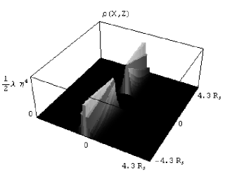
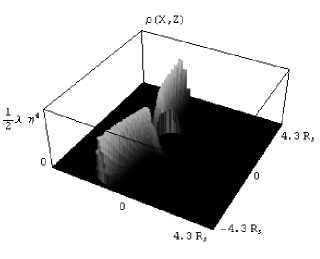
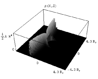
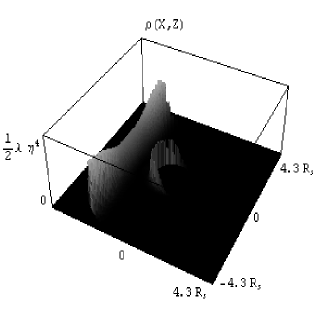
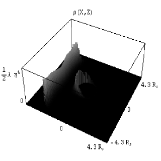
Figure 1: Evolution of the domain wall. The figure shows how the energy density of the wall evolves, explicitly illustrating the separation process and escape of the black hole. The reported simulation refers to the five dimensional case, $d=5$, and a domain wall whose thickness is $1/3$ of the Schwarzschild radius and $v=0.3$.

Acknowledgements. We thank J.J. Blanco-Pillado, H. Kudoh, T. Shiromizu and H. Yoshino for useful discussions and for raising interesting questions. OP acknowledges the kind hospitality of the CCPP at NYU. This work is supported in part by Grant-in-Aid for Scientific Research, Nos. 1604724 and 16740165 and the Japan-U.K. Research Cooperative Program both from Japan Society for Promotion of Science. This work is also supported by the 21st Century COE “Center for Diversity and Universality in Physics” at Kyoto university, from the Ministry of Education, Culture, Sports, Science and Technology of Japan and by Monbukagakusho Grant-in-Aid for Scientific Research(S) No. 14102004 and (B) No. 17340075. A.F. is supported by the JSPS under contract No. P047724. O.P. is supported by the JSPS under contract No. P03193.

References

- (1) Ya.B. Zeldovich, I.D. Novikov, Sov. Astron. Astrophys. J. 10 602 (1967).
- (2) S.W. Hawking, Mon. Not. R. Astron. Soc. 152 75 (1971).
- (3) A. Vilenkin, E.P.S. Shellard, ‘Cosmic Strings and other Topological Defects’, Cambridge University Press (2000).
- (4) M. Christensen, V. P. Frolov, A.L. Larsen, Phys. Rev. D58 (1998) 085008.
- (5) Y. Morisawa, R. Yamazaki, D.Ida, A. Ishibashi, K. Nakao, Phys. Rev. D62 (2000) 084022.
- (6) M. Rogatko, Phys. Rev. D64 (2001) 064014.
- (7) Y. Morisawa, D.Ida, A. Ishibashi, K. Nakao, Phys. Rev. D67 (2003) 025017.
- (8) R. Moderski, M. Rogatko, Phys. Rev. D67 (2003) 024006; Phys. Rev. D69 (2004) 084018.
- (9) K. Freese, G.D. Starkman, D. Stojkovic, Phys. Rev. D72 (2005) 045012.
- (10) N. Arkani-Hamed, S. Dimopoulos and G. R. Dvali, Phys. Lett. B 429, 263 (1998).
- (11) L. Randall and R. Sundrum, Phys. Rev. Lett. 83, 3370 (1999).
- (12) S. Dimopoulos, P.C. Argyres, J. March-Russell, Phys. Lett. B441 (1998) 96.
- (13) S. Dimopoulos and G. Landsberg, Phys. Rev. Lett. 87 (2001) 161602.
- (14) S. B. Giddings and S. Thomas, Phys. Rev. D65 (2002) 056010.
- (15) V. P. Frolov, D. Stojkovic, Phys. Rev. Lett. 89 (2002) 151302.
- (16) D. Stojkovic, Phys. Rev. Lett. 94 (2005) 011603.
- (17) A. Flachi, T. Tanaka, Phys. Rev. Lett. 95 161302 (2005).
- (18) F. R. Tangherlini, Nuovo Cim. B 77, (1963) 636.
- (19) R. C. Myers and M. J. Perry, Annals Phys. 172 (1986) 304.
- (20) J. P. Boyd, ‘Chebyshef and Fourier Spectral Methods’, (2000) Dover.