Cosmological Solutions of Low-Energy Heterotic M-Theory

Abstract

We derive a set of exact cosmological solutions to the $D=4$, $\mathcal{N}=1$ supergravity description of heterotic M-theory. Having identified a new and exact $SU(3)$ Toda model solution, we then apply symmetry transformations to both this solution and to a previously known $SU(2)$ Toda model, in order to derive two further sets of new cosmological solutions. In the symmetry-transformed $SU(3)$ Toda case we find an unusual “bouncing” motion for the M5 brane, such that this brane can be made to reverse direction part way through its evolution. This bounce occurs purely through the interaction of non-standard kinetic terms, as there are no explicit potentials in the action. We also present a perturbation calculation which demonstrates that, in a simple static limit, heterotic M-theory possesses a scale-invariant isocurvature mode. This mode persists in certain asymptotic limits of all the solutions we have derived, including the bouncing solution.

I Introduction

In the past ten years, heterotic M-theory has provided an exciting arena in which to analyse the cosmology and particle physics of our universe Horava:1996ma ; Bandos:1997ui ; Lukas:1998tt ; Brandle:2001ts ; Khoury:2001wf ; Steinhardt:2002ih . Representing the low-energy limit of the strongly-coupled heterotic $E_{8}\times E_{8}$ string, this theory not only combines gravitational, particle and braneworld physics into one unified description, but also possesses a detailed and constrained field-content that cannot be arbitrarily adjusted. Therefore, it retains a definitive and unambiguous relationship to M-theory itself. However, in the $D=4,\mathcal{N}=1$ supergravity description of heterotic M-theory, a number of important questions still remain unanswered. Consider, for example, the simple cosmological situation that occurs when we retain only the dilaton $S$, the universal $T$ modulus, and the field $Z$ describing a single M5 brane. Despite the fact that this leads to vanishing superpotential in four dimensions, the resulting cosmology is highly non-linear and demonstrates quite unexpected behaviour. In Ref. Copeland:2001zp the $S,T,Z$ cosmology was analysed in a truncated limit with all axion fields removed. It was then shown that the scalar corresponding to the M5 brane position must be included in the set of cosmologically significant fields, and this leads to a forcing effect whereby the ambient dimensions change size as the brane moves. Moreover, the frictional forces acting back on the brane are such that it accelerates and then decelerates back to rest, mimicking a time-dependent force of finite duration. This illustrates the unconventional effect of non-standard kinetic terms in the theory, and the means by which the brane can undergo a single displacement by exchanging energy with its environment. In the special situation presented in Ref. Copeland:2001zp this effect can be described exactly using the Toda formalism Kostant:1979qu ; Lukas:1996iq , and the model of Ref. Copeland:2001zp is an $SU(2)$ Toda model.

Given this behaviour, it is interesting to consider whether more complicated trajectories for the M5 brane are possible. For example, not all of the scalar fields were considered in the $SU(2)$ Toda model of Ref. Copeland:2001zp , since the axionic fields were consistently truncated away. This means that only a portion of the full solution-space was explored, and that the $SU(2)$ behaviour is liable to be only an approximation once the axions are restored. Therefore, following on from the work of Ref. Copeland:2001zp , we wish to analyse situations in which additional axionic fields are evolving in conjunction with the brane, and determine whether interesting new behaviours for the M5 brane can occur. In particular, we wish to determine whether an M5 brane can undergo multiple displacements, and even reverse direction in the absence of explicit potentials.

Before embarking on the detailed calculations, we first summarise our results. We uncover a new and exact $SU(3)$ Toda model, in which the M5 brane can undergo two successive displacements in the same direction. That is, the brane spontaneously accelerates twice in response to the other moduli fields to which it is coupled. Applying the symmetries derived in our companion paper Ref. Copeland:2005mk to this model, as well as to the known $SU(2)$ model of Ref. Copeland:2001zp , we obtain two additional sets of new solutions. In the symmetry-transformed $SU(3)$ case the brane can undergo two successive displacements in opposite directions, and so reverse direction and “bounce” without the presence of any explicit potentials in the action. This effect occurs purely through the interaction of non-standard kinetic terms, via the cross-couplings of the various fields, and constitutes an exact supergravity solution that has been rigorously deduced from M-theory. Finally we investigate the generation of density perturbations in these models, and show that heterotic M-theory possesses a scale-invariant isocurvature mode in some of the axion fields. This last result is consistent with the original findings of the pre Big Bang scenario Copeland:1997ug ; Copeland:1998ie and in agreement with the result obtained in Ref. DiMarco:2002eb where it was first shown that the moving brane itself could not generate a scale-invariant perturbation spectrum. Following a conclusion, in an appendix we present the technical details of the $SU(3)$ Toda model derivation.

II The Four-dimensional action

We now review the $D=4,\mathcal{N}=1$ supergravity action presented in Ref. Copeland:2001zp . Recall that this was derived via a compactification of 11D supergravity on the orbifold $S^{1}/\mathbb{Z}_{2}\times CY_{3}$, where $CY_{3}$ denotes a Calabi-Yau three-fold. This leads to two four-dimensional boundary planes separated along a fifth dimension. If the fifth dimension is labelled by a normalised coordinate $z\in[0,1]$, then the boundaries reside at $z=0,1$ respectively and have the charges $q_{0},q_{1}$. A single M5 brane is also included in the space, by wrapping it on a holomorphic 2-cycle of the $CY_{3}$. The brane then appears as a three-brane of charge $q$ that lies parallel to the boundaries, and which can move along the interval. Importantly, the interaction between the boundaries and brane leads to the existence of a static, triple-domain wall BPS solution. One can then consider further reducing on this solution, so as to find a supergravity theory describing slowly varying fluctuations about the static BPS vacuum. This contains the six scalar fields $\beta,\chi,\phi,\sigma,z,\nu$ with the following non-standard kinetic terms

$$\begin{split}S_{4}=-\frac{1}{2\kappa_{4}^{2}}\int_{M_{4}}d^{4}x\sqrt{-g}\left[\frac{1}{2}R+\frac{3}{4}(\partial\beta)^{2}+3e^{-2\beta}(\partial\chi)^{2}+\frac{1}{4}(\partial\phi)^{2}+\frac{1}{4}e^{-2\phi}\left(\partial\sigma+4qz\partial\nu\right)^{2}\right.\\ \left.+\frac{1}{2}qe^{\beta-\phi}(\partial z)^{2}+2qe^{-\beta-\phi}(\partial\nu-\chi\partial z)^{2}\right]\end{split}$$ (1)

Each of these scalars has an underlying significance in terms of the $D=5$ parent theory from which it descends. The scalar $\beta$ is the zero-mode of the $g_{55}$ component in the $D=5$ metric, and measures the separation between the boundaries. Specifically, the separation is given by $\pi\rho e^{\beta}$ in terms of some dimensionful reference size $\pi\rho$. The field $\phi$ represents the orbifold-averaged Calabi-Yau volume, such that the physical size is given by $ve^{\phi}$ in terms of a dimensionful reference volume $v$. The scalars $\sigma,\chi$ originate from the bulk three-form and graviphoton field respectively. The field $z$ measures the position of the bulk brane between the boundaries, with the points $z=0,1$ corresponding to the boundaries. Lastly, the field $\nu$ arises from the self-dual two-form on the brane worldvolume.

This reduction on a BPS solution guarantees that the scalars must group into supersymmetric multiplets described by a supersymmetric action. One can verify that they naturally fall into the pairs $(\phi,\sigma)$,$(\beta,\chi)$,$(z,\nu)$, which are the bosonic components of chiral superfields $S,T,Z$ as follows

$$S=e^{\phi}+qz^{2}e^{\beta}+i\left(\sigma+2qz^{2}\chi\right)\quad,\quad T=e^{\beta}+2i\chi\quad,\quad Z=e^{\beta}z+2i(-\nu+z\chi)$$ (2)

This naturally leads to a Kähler manifold expression for the scalar part of the action

$$S_{4}=-\frac{1}{2\kappa_{4}^{2}}\int d^{4}x\sqrt{-g}\left(\frac{1}{2}R+K_{i\bar{j}}\>\partial_{\mu}{\Phi}^{i}\partial^{\mu}{\bar{\Phi}}^{\bar{j}}\right)$$ (3)

where the superfields are grouped into a coordinate vector $\Phi=(S,T,Z)$, with the complex conjugate coordinates denoted by $\bar{\Phi}$. The Kähler metric $K_{i\bar{j}}$ is given by

$$K_{i\bar{j}}=\frac{\partial^{2}{K}}{\partial{\Phi^{i}}\partial{\bar{\Phi}^{\bar{j}}}}$$ (4)

in terms of the Kähler potential

$$K=-\ln\left[S+\overline{S}-q\frac{(Z+\overline{Z})^{2}}{T+\overline{T}}\right]-3\ln\left(T+\overline{T}\right)$$ (5)

This Kähler potential is computed only to linear-order in the two parameters $\epsilon_{k}$ $(k=1,2)$ defined by

$$\epsilon_{k}=\sum_{i=0}^{k-1}\>\pi\left(\frac{\kappa}{4\pi}\right)^{2/3}\frac{2\pi\rho}{v^{2/3}}\>q_{i}\>e^{\beta-\phi}$$

Here $\kappa$ is the eleven-dimensional Newton constant, and $\pi\rho,v$ are the dimensionful scales mentioned above. The two conditions $\epsilon_{k}\ll 1$ then restrict the accessible regions of moduli-space in which we can trust the four-dimensional effective theory. In addition, the supergravity action Eq. (1) can only be trusted in the limit where stringy $\alpha^{\prime}$ corrections are suitably small, as these corrections introduce higher-derivative terms that we have disregarded.

III Equations of Motion

We now turn to the equations of the motion arising from the action Eq. (1). If we assume a spatially flat Friedmann Robertson Walker (FRW) cosmology for the four-dimensional spacetime, then the metric takes the form

$$ds_{4}^{2}=-e^{2n(\tau)}d\tau^{2}+e^{2\alpha(\tau)}\delta_{ij}dx^{i}dx^{j}$$ (6)

where $i,j=1,\dots,3$, the scale-factor is $\alpha(\tau)$, and $n(\tau)$ represents a gauge freedom in the choice of time coordinate. Denoting a $\tau$ derivative by an overdot, and assuming all fields are purely functions of $\tau$, one obtains the Einstein field equations

$$-3\dot{\alpha}^{2}+\frac{1}{4}\dot{\phi}^{2}+\frac{3}{4}\dot{\beta}^{2}+\frac{1}{2}qe^{\beta-\phi}\dot{z}^{2}+3e^{-2\beta}\dot{\chi}^{2}+ \frac{1}{4}e^{-2\phi}\left(\dot{\sigma}+4qz\dot{\nu}\right)^{2}+2qe^{-\beta-\phi}(\dot{\nu}-\chi\dot{z})^{2}=0$$ (7)

$$2\ddot{\alpha}+(3\dot{\alpha}-2\dot{n})\dot{\alpha}+\frac{1}{4}\dot{\phi}^{2}+\frac{3}{4}\dot{\beta}^{2}+\frac{1}{2}qe^{\beta-\phi}\dot{z}^{2}+3e^{-2\beta}\dot{\chi}^{2}+ \frac{1}{4}e^{-2\phi}\left(\dot{\sigma}+4qz\dot{\nu}\right)^{2}+2qe^{-\beta-\phi}(\dot{\nu}-\chi\dot{z})^{2}=0$$ (8)

the $\phi,\beta,z$ equations of motion

$$\ddot{\phi}+(3\dot{\alpha}-\dot{n})\dot{\phi}+qe^{\beta-\phi}\dot{z}^{2}+(\dot{\sigma}+4qz\dot{\nu})^{2}e^{-2\phi}+4q(\dot{\nu}-\chi\dot{z})^{2}e^{-\beta-\phi} =0$$ (9)

$$3\ddot{\beta}+3(3\dot{\alpha}-\dot{n})\dot{\beta}-qe^{\beta-\phi}\dot{z}^{2}+12\dot{\chi}^{2}e^{-2\beta}+4q(\dot{\nu}-\chi\dot{z})^{2}e^{-\beta-\phi} =0$$ (10)

$$\frac{d}{d\tau}\left\{\left[e^{\beta-\phi}\dot{z}-4\chi(\dot{\nu}-\chi\dot{z})e^{-\beta-\phi}\right]e^{3\alpha-n}\right\}e^{n-3\alpha}-2\dot{\nu}(\dot{\sigma}+4qz\dot{\nu})e^{-2\phi} =0$$ (11)

and the $\sigma,\nu,\chi$ equations of motion

$$\frac{d}{d\tau}\left\{\>\left[\>(\dot{\sigma}+4qz\dot{\nu})e^{-2\phi}\>\right]e^{3\alpha-n}\>\right\} =0$$ (12)

$$\frac{d}{d\tau}\left\{\left[z(\dot{\sigma}+4qz\dot{\nu})e^{-2\phi}+2(\dot{\nu}-\chi\dot{z})e^{-\beta-\phi}\right]e^{3\alpha-n}\right\} =0$$ (13)

$$\frac{d}{d\tau}\left[\>(3e^{-2\beta}\dot{\chi})e^{3\alpha-n}\>\right]e^{n-3\alpha}+2q\dot{z}(\dot{\nu}-\chi\dot{z})e^{-\beta-\phi} =0$$ (14)

As we cannot exactly solve these equations of motion, we will utilise the following two solution methods. Firstly, we search for specialised solutions that occur when the equations are truncated, usually by setting certain combinations of fields to zero. This will allow us to recover the known $SU(2)$ Toda model of Ref. Copeland:2001zp , as well as a previously undiscovered $SU(3)$ Toda model. Secondly, we will utilise the scalar-field symmetry transformations that were derived in our recent companion paper Ref. Copeland:2005mk . That is, we will apply these symmetry transformations to the fields of the $SU(2)$ and $SU(3)$ Toda models in turn, and so derive two new solutions to the equations of motion. We will find that in these new solutions the M5 brane can evolve in far more complicated ways than has previously been seen.

IV Review of the $SU(2)$ Toda Model

We now briefly recall the behaviour of the $SU(2)$ Toda model found in Ref. Copeland:2001zp . This will prove useful because the $SU(2)$ model exhibits features that persist in all the solutions we will present, and so will illuminate the discussions to come. In addition, it is worthwhile studying this model in order to understand how symmetry-transformations will affect it.

IV.1 The $SU(2)$ Toda Model Solutions

The $SU(2)$ model can be derived by choosing the axions to satisfy $\sigma,\nu=\mathrm{constant},\chi=0$. The remaining fields $\alpha,\phi,\beta,z$ can then be solved for exactly, essentially due to the fact that the field $z$ satisfies the conservation law

$$e^{\beta-\phi+3\alpha-n}\dot{z}=\mathrm{constant}$$ (15)

Namely, inserting this result back into the remaining equations of motion yields a closed set of equations in $\alpha,\beta,\phi$ which can be solved in isolation. In particular, these equations can be reformulated in terms of the motion of a “particle” with coordinates $\mbox{\boldmath$\alpha$}=(\alpha,\beta,\phi)$ which roams over a three-dimensional space and experiences an exponential potential $U$. These equations take the form

$$\frac{d}{d\tau}\left(EG\mbox{\boldmath$\dot{\alpha}$}\right)+E^{-1}\frac{\partial U}{\partial\mbox{\boldmath$\alpha$}}=0\quad,\quad\frac{1}{2}E\mbox{\boldmath$\dot{\alpha}$}^{T}G\>\mbox{\boldmath$\dot{\alpha}$}+E^{-1}U=0$$ (16)

which can be derived by variation of $\mbox{\boldmath$\alpha$},E$ from the simpler particle Lagrangian

$$\mathcal{L}=\frac{1}{2}E\mbox{\boldmath$\dot{\alpha}$}^{T}G\>\mbox{\boldmath$\dot{\alpha}$}-E^{-1}U$$ (17)

Here we have defined a moduli-space metric $G=\mathrm{diag}(-3,\frac{3}{4},\frac{1}{4})$ of Minkowski signature, and a particle-worldline metric $E=e^{-n+\mathbf{d}\cdot\mbox{\boldmath$\alpha$}}$ where $\mathbf{d}=(3,0,0)$ is a dimension vector that gives the number of spatial dimensions associated to the scale-factor $\alpha$. The function $E$ thus encodes the arbitrary choice of time parameterisation of the worldline, with its variation in the Lagrangian naturally producing an energy conservation constraint. Finally, the moduli-space potential $U=U_{1}$ is given by

$$U_{1} =\frac{1}{2}u_{1}^{2}\>\mathrm{exp}\left(\mathbf{q}_{1}\cdot\mbox{\boldmath$\alpha$}\right)\quad,\quad\mathbf{q}_{1}=(0,-1,1)$$ (18)

where $u_{1}^{2}$ is a positive constant. Up to a constant length rescaling, the vector $\mathbf{q}_{1}$ defines the single, simple root-vector of the Lie algebra $SU(2)$, and so the Lagrangian Eq. (17) defines an $SU(2)$ Toda model. This is an exactly integrable system, and in the proper-time gauge $n=0$ one finds the general solution:

$${\mbox{\boldmath$\alpha$}}-{\mbox{\boldmath$\alpha$}}_{0}={\bf p}_{i}\ln\left|\frac{t-t_{0}}{T}\right|+\left({\bf p}_{f}-{\bf p}_{i}\right)\ln\left(1+\left|\frac{t-t_{0}}{T}\right|^{-\delta}\right)^{-1/\delta}$$ (19)

$$z-z_{0}=d\left(1+\left|\frac{t-t_{0}}{T}\right|^{\delta}\right)^{-1}$$ (20)

$$~{}{\bf p}_{\gamma}G{\bf p}_{\gamma}=0\quad,\quad{\bf p}_{\gamma}\cdot{\bf d}=1\quad,\quad{\bf q}_{1}\cdot{\mbox{\boldmath$\alpha$}}_{0}=\ln\left(\frac{qd^{2}<{\bf q}_{1},{\bf q}_{1}>}{8}\right)\quad,\quad\delta=-{\bf q}_{1}\cdot{\bf p}_{i}\quad,\quad{\bf p}_{f}-{\bf p}_{i}=\delta\frac{2G^{-1}{\bf q}_{1}}{<{\bf q}_{1},{\bf q}_{1}>}$$ (21)

Here the subscript $\gamma$ takes the values $\gamma=i,f$, and the scalar product $<\cdot,\cdot>$ is defined by $<{\bf a},{\bf b}>={\bf a}^{T}G^{-1}{\bf b}$. Note that the constraints in Eq. (21) must be enforced so that Eqs. (19)-(20) are indeed the correct field solutions. Once this is done, the solution describes a transition between two asymptotically free-field states. That is, the initial field velocities are equal to the “expansion power” constants ${\bf p}_{i}=(1/3,p_{\beta,i},p_{\phi,i})$, the final field velocities are equal to the constants ${\bf p}_{f}=(1/3,p_{\beta,f},p_{\phi,f})$, and the nonsupersymmetric second term in Eq. (19) forces a smooth acceleration between these “rolling-radii” (rr) regimes. In fact, the underlying reason for this ${\bf p}_{i}\rightarrow{\bf p}_{f}$ interpolation is the motion of the brane itself, which according to Eq. (20) is at rest in the extreme limits, but borrows kinetic energy from $\beta,\phi$ and moves significantly at the intermediate time $t-t_{0}\approx T$. For the sake of concreteness, we now present the explicit form of the solutions by inserting the various vector quantities. This gives

$$\alpha-\alpha_{0} =\frac{1}{3}\ln\left|\frac{t-t_{0}}{T}\right|$$

$$\beta-\beta_{0} =p_{\beta,i}\ln\left|\frac{t-t_{0}}{T}\right|+(p_{\beta,f}-p_{\beta,i})\ln\left(1+\left|\frac{t-t_{0}}{T}\right|^{-\delta}\right)^{-1/\delta}$$

$$\phi-\phi_{0} =p_{\phi,i}\ln\left|\frac{t-t_{0}}{T}\right|+(p_{\phi,f}-p_{\phi,i})\ln\left(1+\left|\frac{t-t_{0}}{T}\right|^{-\delta}\right)^{-1/\delta}$$

These are subject to the relations

$$\delta=p_{\beta,i}-p_{\phi,i}\quad,\quad\beta_{0}-\phi_{0}=\ln\left(\frac{3}{2qd^{2}}\right)\quad,\quad\left(\begin{array}[]{c}p_{\beta,f}\\ p_{\phi,f}\end{array}\right)=\frac{1}{2}\left(\begin{array}[]{rr}1&1\\ 3&-1\end{array}\right)\left(\begin{array}[]{c}p_{\beta,i}\\ p_{\phi,i}\end{array}\right)$$

as well as the “ellipse” constraint

$$3p_{\beta,i}^{2}+p_{\phi,i}^{2}=\frac{4}{3}$$ (22)

Notice, in fact, that if we enforce the constraint that fixes $(p_{\beta,f},p_{\phi,f})$ in terms of $(p_{\beta,i},p_{\phi,i})$ then the final expansion powers $(p_{\beta,f},p_{\phi,f})$ are automatically guaranteed to lie on the same ellipse. The interpretation of this ellipse condition is relatively simple, and can be illustrated in a phase-plane diagram as follows. Consider drawing a 2D plot where the horizontal axis corresponds to $d\beta/du$ (with $u\equiv 3\alpha$) and the vertical axis to $d\phi/du$. Then the constants $(p_{\beta,\gamma},p_{\phi,\gamma})$, where $\gamma=i,f$, are the asymptotic values of $d\beta/du$ and $d\phi/du$. Thus, they correspond to the values attained in the plane at the extreme endpoints of the phase-plane trajectory. Hence, according to Eq. (22) and the constraints, the trajectory traced out in the phase-plane must begin and end at two different points on a single, fixed ellipse drawn in that plane. These phase-plane plots, or “ellipse diagrams” as we shall call them, will prove to be extremely useful in exhibiting the behaviour of the system diagrammatically. This is because the shape and curves of the trajectories in these diagrams tell us very graphically about the brane motion and changes to the axions.

IV.2 Analysis and Validity of the $SU(2)$ Toda Model

To exhibit the behaviour of the fields, we now plot an ellipse diagram. This proves to be far more intuitive and useful than following the behaviour of all fields individually. Before doing this, we must recognise that the solutions in Eq. (19) are valid over two disconnected time ranges given by

$$t\in\left\{\begin{array}[]{clll}\left(-\infty,t_{0}\right)\;,&(-)\;{\rm branch}\\ \left(t_{0},+\infty\right)\;,&(+)\;{\rm branch}\end{array}\right.$$ (25)

where the time $t=t_{0}$ corresponds to a curvature singularity. Consequently, there are two different notions of “early” and “late” built into the solutions, depending on the choice of branch. For example, although $t=t_{0}$ corresponds to a past singularity in the $(+)$ branch, it corresponds to a future singularity from the perspective of the $(-)$ branch. The $(-)$ branch is, in fact, an example of a pre Big Bang (PBB) era, which is automatically undergoing superluminal deflation.

Therefore, to avoid confusion we must always pick a particular branch, and take care with what constitutes early and late behaviour. In particular, the $\mathbf{p}_{i}$ constants only correspond to an “initial” set of expansion powers as implied by the subscript if they satisfy

$$\delta=p_{\beta,i}-p_{\phi,i}\left\{\begin{array}[]{c}>0\quad(-)\>{\rm branch}\\ <0\quad(+)\>{\rm branch}\end{array}\right.$$ (28)

That is, only those powers satisfying this condition can ever be early time states of the system. In Fig. 1 we have plotted some representative trajectories on the $(-)$ branch. Note that the fields $\beta,\phi$ start at a single point on the ellipse, with their initial powers corresponding to that sector with $\delta>0$. On the negative branch this “early” time state corresponds to the infinitely negative past $t-t_{0}\rightarrow-\infty$. The fields then evolve such that the effective trajectory in the plane is a straight line. This linear behaviour is a consequence of the relation $3d\beta/du+d\phi/du\propto\mathrm{constant}$, and this in turn is possible because all the axions have been truncated away. The trajectory then ends on the opposite sector of the ellipse, ending up in a “late” time state as $t-t_{0}\rightarrow 0$ from below. This directed evolution between parts of the ellipse cannot be reversed unless we switch the branch from $(-)$ to $(+)$, so the accessible early-time states of the system are fixed by the choice of the branch. Thus, interesting physical results will sometimes necessitate choosing one branch over another.

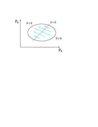
Figure 1: Figure to show the linear mapping across the ellipse, with the direction fixed by the choice of time branch. If we pick a candidate set of expansion powers satisfying $\delta>0$, then these are indeed available early-time states on the $(-)$ branch. States satisfying $\delta<0$ are not available at early time; instead, they are the late time states that the system evolves into. This is all reversed on the $(+)$ branch.

To complete this section, we now comment on the validity of these $SU(2)$ Toda solutions. Recall that the four-dimensional action Eq. (1) is known only as a power series, with five-dimensional gravitational corrections measured in powers of the $\epsilon_{k}$ ($k=1,2$). In the above model one finds that

$$\epsilon_{k}\sim\left\{\begin{array}[]{lll }|t-t_{0}|^{+\delta}&\rightarrow\infty\quad\text{early time}\\ |t-t_{0}|^{-\delta}&\rightarrow\infty\quad\text{late time}\end{array}\right.$$ (31)

This divergence is due to the fact that the coupling of the bulk brane to $\beta,\phi$ is itself proportional to the $\epsilon_{k}$, so that when the brane moves the system is necessarily driven to a five-dimensional limit in both asymptotic regimes. This will cause the four-dimensional theory to break down, and with it the solutions Eq. (19). This divergence is in fact familiar from PBB cosmology where the addition of the dilatonic axion to the dilaton-moduli system causes the same problem. A more insidious problem, however, is that even at intermediate times one cannot make $\epsilon_{k}\ll 1$ whilst simultaneously fitting the entire $z$ displacement profile within the physical orbifold extent $z\in[0,1]$. Say, for example, that we search for the minimum value of the $\epsilon_{k}$ parameters. One can verify that this occurs at precisely the time $t-t_{0}=T$, and at this time the ellipse trajectory intersects the line $\delta=0$. The magnitude at the minimum is then

$$\epsilon_{k}|_{\mathrm{min}}\sim\frac{1}{d^{2}}$$

Evidently, $d\gg 1$ is now required in order to make this small. Having made this choice, there will be a finite period of time, depending on the value of $d$, where the $\epsilon_{k}$ are small and our solutions, Eq. (19), are valid. This period ends with the rapid collision of the brane with the boundary which, of course, also invalidates the above analytical solutions. (For a discussion of the evolution after the collision see Ref. Gray:2003vk ). The limitations on the validity of these solutions, both due to the $\epsilon_{k}$ constraint and brane-boundary collision, may be viewed as a disadvantage and one may ask whether other solutions with a larger range of validity exist. We will show that this is indeed the case for some of the new solutions to be discussed below.

V The $SU(3)$ Toda Model

After reviewing the $SU(2)$ model at some length, we will now present an entirely new $SU(3)$ solution. This proves to be significantly more complicated than the $SU(2)$ Toda model, as we might expect from the fact that the Lie group $SU(3)$ is more complicated in structure than $SU(2)$. We will find that the $SU(3)$ solutions are fundamentally controlled by two influences, one due to the motion of the M5 brane and the other due to changes in $\chi$. This leads to new, characteristic trajectories in the ellipse diagrams. In particular, the coupling between $z$ and $\chi$ allows the M5 brane to undergo two successive displacements in the same direction. This generalises the behaviour of the old $SU(2)$ case, and demonstrates that the brane can undergo repetitious displacement behaviour.

V.1 The $SU(3)$ Toda Model Solutions

To derive the $SU(3)$ Toda model, one chooses the axions to satisfy

$$\dot{\nu}-\chi\dot{z}=\dot{\sigma}+4qz\dot{\nu}=0$$ (32)

This effectively sets two of the terms in the action to zero for all time, without forcing any of the fields or their derivatives to be individually zero. To see that this corresponds to an $SU(3)$ Toda model we impose Eq. (32), and note that the $z$ and $\chi$ equations are now total derivatives

$$\frac{d}{d\tau}\left[e^{\beta-\phi+3\alpha-n}\dot{z}\right]=\frac{d}{d\tau}\left[e^{-2\beta+3\alpha-n}\dot{\chi}\right]=0$$

These can be immediately integrated to give constants of the motion. Inserting these conservation laws back into the remaining equations of motion then yields a closed set of equations in $\alpha,\beta,\phi$ that can again be derived from the particle Lagrangian

$$~{}\mathcal{L}=\frac{1}{2}E\mbox{\boldmath$\dot{\alpha}$}^{T}G\>\mbox{\boldmath$\dot{\alpha}$}-E^{-1}U$$ (33)

The quantities $\mbox{\boldmath$\alpha$},G,E$ remain unchanged from the $SU(2)$ Toda model, but the potential is modified to $U=U_{1}+U_{2}$, with

$$U_{1} =\frac{1}{2}u_{1}^{2}\>\mathrm{exp}\left(\mathbf{q}_{1}\cdot\mbox{\boldmath$\alpha$}\right)\quad,\quad\mathbf{q}_{1}=(0,-1,1)$$

$$U_{2} =\frac{1}{2}u_{2}^{2}\>\mathrm{exp}\left(\mathbf{q}_{2}\cdot\mbox{\boldmath$\alpha$}\right)\quad,\quad\mathbf{q}_{2}=(0,2,0)$$

This means that the effective particle motion of $\alpha$ is now subjected to two exponential forces. To be a Toda model, a precise relationship must exist between the orientations and lengths of the vectors defined by the $\mathbf{q}_{i}$. Consider the following matrix

$$<\mathbf{q}_{i},\mathbf{q}_{j}>=\frac{8}{3}\cdot\left(\begin{array}[]{cc}2&-1\\ -1&2\\ \end{array}\right)$$ (36)

where the scalar product is once again defined by $<{\bf a},{\bf b}>={\bf a}^{T}G^{-1}{\bf b}$. The right hand side of Eq. (36) happens to be a constant multiple of the Cartan matrix of the $SU(3)$ Lie algebra, so that up to a constant length rescaling the vectors $\mathbf{q}_{1},\mathbf{q}_{2}$ are identical to the two simple root-vectors of $SU(3)$. Thus, the model is an exactly integrable $SU(3)$ Toda model. In particular, an exact, analytical description of the behaviour is now accessible if we choose a basis for the moduli-space that is adapted to the $SU(3)$ root-vectors. This decouples the equations of motion and allows them to be readily solved, the complicated details of which are reserved for Appendix A. The proper-time solutions for the fields in the gauge $n=0$ are then given by

$${\mbox{\boldmath$\alpha$}}-{\mbox{\boldmath$\alpha$}}_{0}={\bf p}_{i}\ln\left|\frac{t-t_{0}}{T}\right| +\left({\bf p}_{f}-{\bf p}_{i}\right)\ln\left[1+\left|\frac{t-t_{0}}{T}\right|^{-\delta}\left(1+\theta_{z}^{2}\left|\frac{t-t_{0}}{T_{\beta}}\right|^{-\delta_{\beta}}\right)\right]^{-1/\delta}$$

$$+ \left({\bf p}_{f}^{(\chi)}-{\bf p}_{i}\right)\ln\left[1+\left|\frac{t-t_{0}}{T_{\beta}}\right|^{-\delta_{\beta}}\left(1+\theta_{\chi}^{2}\left|\frac{t-t_{0}}{T}\right|^{-\delta}\right)\right]^{-1/\delta_{\beta}}$$ (37)

$$z-z_{0} =d\left(1+\left|\frac{t-t_{0}}{T}\right|^{\delta}+\theta_{z}^{2}\left|\frac{t-t_{0}}{T_{\beta}}\right|^{-\delta_{\beta}}\right)^{-1}\cdot\left(1+\theta_{z}\left|\frac{t-t_{0}}{T_{\beta}}\right|^{-\delta_{\beta}}\right)$$ (38)

$$\chi-\chi_{0} =d_{\chi}\left(1+\left|\frac{t-t_{0}}{T_{\beta}}\right|^{\delta_{\beta}}+\theta_{\chi}^{2}\left|\frac{t-t_{0}}{T}\right|^{-\delta}\right)^{-1}\cdot\left(1+\theta_{\chi}\left|\frac{t-t_{0}}{T}\right|^{-\delta}\right)$$ (39)

The constants are subject to the following two sets of “$SU(2)$-like” constraints

$${\bf p}_{\gamma}G{\bf p}_{\gamma} =0 {\bf p}_{\gamma}\cdot{\bf d} =1 \delta =-{\bf q}_{1}\cdot{\bf p}_{i} {\bf q}_{1} \cdot{\mbox{\boldmath$\alpha$}}_{0}=\ln\left(\frac{qd^{2}<{\bf q}_{1},{\bf q}_{1}>}{8}\right)$$ (40)

$${\bf p}_{f}^{(\chi)}G{\bf p}_{f}^{(\chi)} =0 {\bf p}_{f}^{(\chi)}\cdot{\bf d} =1 \delta_{\beta} =-{\bf q}_{2}\cdot{\bf p}_{i} {\bf q}_{2} \cdot\left[{\mbox{\boldmath$\alpha$}}_{0}-{\bf p}_{i}\ln\left|\frac{T}{T_{\beta}}\right|\right]=\ln\left(\frac{3d_{\chi}^{2}<{\bf q}_{2},{\bf q}_{2}>}{4}\right)$$ (41)

where $\gamma=i,f$, and the scalar product $<\cdot,\cdot>$ is again defined by $<{\bf a},{\bf b}>={\bf a}^{T}G^{-1}{\bf b}$. Moreover, ${\bf p}_{f}$, ${\bf p}_{f}^{(\chi)}$and ${\bf p}_{i}$ are related by the two $SU(2)$ maps

$${\bf p}_{f}-{\bf p}_{i}=\delta\frac{2G^{-1}{\bf q}_{1}}{<{\bf q}_{1},{\bf q}_{1}>}\quad,\quad{\bf p}_{f}^{(\chi)}-{\bf p}_{i}=\delta_{\beta}\frac{2G^{-1}{\bf q}_{2}}{<{\bf q}_{2},{\bf q}_{2}>}$$ (42)

Finally, the fractional quantities $\theta_{z},\theta_{\chi}$ are fixed according to

$$\theta_{z}=\frac{{\bf q}_{1}\cdot{\bf p}_{i}}{({\bf q}_{1}+{\bf q}_{2})\cdot{\bf p}_{i}}\quad,\quad\theta_{\chi}=\frac{{\bf q}_{2}\cdot{\bf p}_{i}}{({\bf q}_{1}+{\bf q}_{2})\cdot{\bf p}_{i}}$$ (43)

These satisfy $0\leq\theta_{z},\theta_{\chi}\leq 1$ and $\theta_{z}+\theta_{\chi}=1$. For clarity, we now present the solutions and constraints for $\alpha$ in component fields. These read

$$\alpha-\alpha_{0}=\frac{1}{3}\ln\left|\frac{t-t_{0}}{T}\right|$$ (44)

$$\beta-\beta_{0}=p_{\beta,i}\ln\left|\frac{t-t_{0}}{T}\right| +(p_{\beta,f}-p_{\beta,i})\ln\left[1+\left|\frac{t-t_{0}}{T}\right|^{-\delta}\left(1+\theta_{z}^{2}\left|\frac{t-t_{0}}{T_{\beta}}\right|^{-\delta_{\beta}}\right)\right]^{-1/\delta}$$

$$+(p_{\beta,f}^{(\chi)}-p_{\beta,i})\ln\left[1+\left|\frac{t-t_{0}}{T_{\beta}}\right|^{-\delta_{\beta}}\left(1+\theta_{\chi}^{2}\left|\frac{t-t_{0}}{T}\right|^{-\delta}\right)\right]^{-1/\delta_{\beta}}$$ (45)

$$\phi-\phi_{0}=p_{\phi,i}\ln\left|\frac{t-t_{0}}{T}\right| +(p_{\phi,f}-p_{\phi,i})\ln\left[1+\left|\frac{t-t_{0}}{T}\right|^{-\delta}\left(1+\theta_{z}^{2}\left|\frac{t-t_{0}}{T_{\beta}}\right|^{-\delta_{\beta}}\right)\right]^{-1/\delta}$$ (46)

$$+(p_{\phi,f}^{(\chi)}-p_{\phi,i})\ln\left[1+\left|\frac{t-t_{0}}{T_{\beta}}\right|^{-\delta_{\beta}}\left(1+\theta_{\chi}^{2}\left|\frac{t-t_{0}}{T}\right|^{-\delta}\right)\right]^{-1/\delta_{\beta}}$$ (47)

The constants $\delta,p_{\beta,i},t_{0},T,d,z_{0}$ all occurred in the previous $SU(2)$ solutions and so are familiar. The three new constants are given by $T_{\beta},\chi_{0},d_{\chi}$ with the remainder constrained according to

$$\delta_{\beta}=-2p_{\beta,i}\quad,\quad\theta_{z}=1-\theta_{\chi}=\frac{\delta}{\delta+\delta_{\beta}}\quad,\quad\beta_{0}=\ln\left(2d_{\chi}\right)+p_{\beta,i}\ln\left|\frac{T}{T_{\beta}}\right|\quad,\quad\beta_{0}-\phi_{0}=\ln\left(\frac{3}{2qd^{2}}\right)$$

$$\left(\begin{array}[]{c}p_{\beta,f}\\ p_{\phi,f}\end{array}\right)=\frac{1}{2}\left(\begin{array}[]{rr}1&1\\ 3&-1\end{array}\right)\left(\begin{array}[]{c}p_{\beta,i}\\ p_{\phi,i}\end{array}\right)\quad,\quad\left(\begin{array}[]{c}p_{\beta,f}^{(\chi)}\\ p_{\phi,f}^{(\chi)}\end{array}\right)=\left(\begin{array}[]{rr}-1&0\\ 0&1\end{array}\right)\left(\begin{array}[]{c}p_{\beta,i}\\ p_{\phi,i}\end{array}\right)$$

Before discussing these $SU(3)$ solutions in more detail, we should also comment on the solutions for the additional fields $\nu,\sigma$ satisfying Eq. (32). It transpires that the $\sigma$ solution involves a non-elementary integral, and so cannot be presented analytically. However, its behaviour can always be computed numerically. On the other hand, the field $\nu$ takes the simple form

$$\nu-\nu_{0}=d_{\nu}\left(1+\left|\frac{t-t_{0}}{T}\right|^{\delta}+\theta_{z}^{2}\left|\frac{t-t_{0}}{T_{\beta}}\right|^{-\delta_{\beta}}\right)^{-1}\cdot\left(\theta_{\nu}+\theta_{z}\left|\frac{t-t_{0}}{T_{\beta}}\right|^{-\delta_{\beta}}\right)$$ (48)

subject to the conditions

$$d_{\nu}\equiv d\left(\chi_{0}+d_{\chi}\right)\quad,\quad\theta_{\nu}\equiv\chi_{0}\left(\chi_{0}+d_{\chi}\right)^{-1}$$ (49)

Interestingly, the field $\nu$ can reverse field-velocity midway through its evolution, and so “turn-around” or “bounce”. This peculiar effect will have important ramifications when we transform the $SU(3)$ solutions later on, for it will allow the brane field $z$ to bounce as well.

V.2 Analysis and Validity of the $SU(3)$ Toda Model

There are two distinct $SU(2)$ models embedded non-trivially in these solutions. If we take the limit $T_{\beta}\gg T$ then the early-time behaviour of the fields is formally identical to the solutions Eq. (19) of the previous section. If instead we reverse the temporal sequence by choosing $T_{\beta}\ll T$ then the early time behaviour is another three-field $SU(2)$ model involving $\chi$ as the axion. These two models are not decoupled as they would be in the $SU(2)\times SU(2)$ Toda case, but instead are non-trivially mixed inside the $SU(3)$ model. Only in extreme cases can we discern the underlying $SU(2)$ components, and so at a general, intermediate time there will not be a clean separation of the effects of the $z$ and $\chi$ motions. Indeed, these two embedded behaviours couple and compete with one another, and attempt to drive the expansion powers according to the two conflicting processes

$${\bf p}_{i}\rightarrow{\bf p}_{f}\quad,\quad{\bf p}_{i}\rightarrow{\bf p}_{f}^{(\chi)}$$

In general, this means that neither ${\bf p}_{f}$ nor ${\bf p}_{f}^{(\chi)}$ individually succeed in becoming the actual expansion powers that the system adopts at late-time. However, the system may spend some part of its evolution at intermediate rolling-radii states where it adopts these powers temporarily. The true late-time rolling-radii states ${\bf p}_{f}^{\prime}$ are in fact determined from a “combined” relation given by

$$~{}{\bf p}_{f}^{\prime}-{\bf p}_{i}=(\delta+\delta_{\beta})\frac{2G^{-1}{\bf q}}{<{\bf q},{\bf q}>}\quad,\quad{\bf q}={\bf q}_{1}+{\bf q}_{2}$$ (50)

Notice that the final states are computed as if the system followed an ordinary $SU(2)$ model with a combined parameter $\delta+\delta_{\beta}$. However, the intermediate behaviour strongly deviates from any such simple $SU(2)$ evolution, and we should treat Eq. (50) merely as a formal tool for deducing the rolling-radii endpoints of the trajectory.

To see this clearly, we plot the field behaviour on the ellipse as we did in Section IV (see Fig. 2). Again, the solutions break in $(\pm)$ branches, with $\mathbf{p}_{i}$ corresponding to the early-time expansion powers only if they simultaneously satisfy the two inequalities

$$\delta,\delta_{\beta}>0\quad{\rm on}\quad(-)\quad,\quad\delta,\delta_{\beta}<0\quad{\rm on}\quad(+)$$ (51)

The additional $\delta_{\beta}$ condition restricts the accessible early-time powers to a narrower range of states compared to the $SU(2)$ model. In Fig. 3 we also plot the displacements of $z$ and the $\chi$ axion. This illustrates the important fact that the fields $z,\chi$ can undergo two successive displacements, since each is coupled to the time-development of the other.

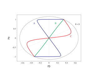
Figure 2: A typical set of $SU(3)$ trajectories. Curve A has two horizontal lines and one diagonal line, and so contains two $\chi$ displacements and one $z$ displacement. Curve B represents a special, degenerate case for which both $z$ and $\chi$ evolve at once and mimic a single field. Curve C has two diagonal lines and one horizontal line, and so contains two $z$ motions separated by a $\chi$ displacement. All intermediate cases between these curves are possible.

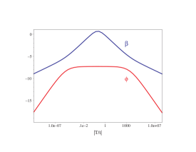
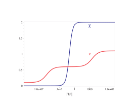
Figure 3: An interesting example of the field evolution. The left hand plot shows the fields $\beta$ and $\phi$. The kinks in these curves are caused by the displacements of $z$ and $\chi$, which are shown in the right hand plot. Notice that $z$ moves twice in succession.

To complete this section, we now comment on the validity of these $SU(3)$ Toda solutions. One can show that

$$~{}e^{\beta-\phi}=\frac{3}{2qd^{2}}\left|\frac{t-t_{0}}{T}\right|^{\delta}\cdot\frac{\left[1+\left|\frac{t-t_{0}}{T}\right|^{-\delta}\left(1+\theta_{z}^{2}\left|\frac{t-t_{0}}{T_{\beta}}\right|^{-\delta_{\beta}}\right)\right]^{2}}{1+\left|\frac{t-t_{0}}{T_{\beta}}\right|^{-\delta_{\beta}}\left(1+\theta_{\chi}^{2}\left|\frac{t-t_{0}}{T}\right|^{-\delta}\right)}$$ (52)

Using this, one can easily verify that in the asymptotic limits

$$\epsilon_{k}\sim\left|\frac{t-t_{0}}{T}\right|^{+\delta}\rightarrow\infty\quad\text{ at early time}\quad,\quad\epsilon_{k}\sim\left|\frac{t-t_{0}}{T_{\beta}}\right|^{-\delta_{\beta}}\rightarrow\infty\quad\text{ at late time}$$

Notice that this follows only because $\delta,\delta_{\beta}$ are both positive (negative) on the negative (positive) time-branch. Consequently, the $SU(3)$ solutions cannot be trusted asymptotically, as with the previous $SU(2)$ solutions of Section IV. Further investigation of Eq. (52) also reveals that it can never be made smaller than the leading coefficient, which is of order $1/qd^{2}$. This demonstrates that the smallest attainable value of the $\epsilon_{k}$ is given by

$$\epsilon_{k}|_{\mathrm{min}}\sim\frac{1}{d^{2}}$$ (53)

Hence, to achieve $\epsilon_{k}\ll 1$ the solutions require us to take $d\gg 1$ and allow the brane to leave the orbifold interval. As such, the $SU(3)$ model has similar problems to the $SU(2)$ model. Of course, as long as we are interested in relatively short timescales, and always concentrate on the brane behaviour inside of the interval but away from the boundaries (and the collision) then no particular problem is posed. Away from the boundaries the $SU(3)$ solutions with $d\gg 1$ are reliable for a short time, and the fact that the brane must eventually leave the interval does not change this fact. Hence, there are always regions where all fields are evolving in an $\epsilon_{k}\ll 1$ regime with the brane inside the interval.

However, it would obviously be valuable if these regions could be extended to cover the entire displacement profile of the brane, such that the brane moves and comes to rest while remaining inside the interval with $\epsilon_{k}\ll 1$ throughout. Although this is impossible with the $SU(3)$ solutions themselves, when we come to symmetry-transform the $SU(3)$ solutions we will find circumstances under which $d<1$ and $\epsilon_{k}\ll 1$ simultaneously.

VI Application of the Symmetries

We now apply the symmetries presented in our companion paper Ref. Copeland:2005mk to the $SU(2)$ and $SU(3)$ models in turn. (For previous work in this area, also see Ref. deCarlos:2004yv ). These symmetries mix the scalar fields together in new combinations, and yet leave the action Eq. (1) invariant. Consequently, the new time-dependent combinations for the fields that emerge, no matter how complicated, still solve the equations of motion. The seven-dimensional symmetry group $G$ is a maximal parabolic subgroup of $Sp(4,\mathbb{R})$ given by

$$~{}G=SL(2,\mathbb{R})\ltimes SU(1,2)/U(2)$$ (54)

where $\ltimes$ denotes a semidirect product. The scalar-field space is then the group manifold $\mathcal{M}\cong Sp(4,\mathbb{R})/U(2)$, but equipped with a nonhomogeneous Riemannian metric such that the total symmetry group fills out only $G$ and not the whole of $Sp(4,\mathbb{R})$. There are seven, distinct types of transformations $L^{i}$ that can be applied to the scalar fields, each one controlled by a continuously adjustable real constant $c_{i}$. These are given by

$$~{}L^{1} :\quad\beta\rightarrow\beta+c_{1} \chi\rightarrow\chi\>e^{c_{1}} z\rightarrow z\>e^{-c_{1}/2} \nu\rightarrow\nu\>e^{c_{1}/2}$$

$$L^{2} :\quad e^{\beta}\rightarrow\frac{e^{\beta}}{(1+c_{2}\chi)^{2}+\frac{1}{4}c_{2}^{2}e^{2\beta}} \chi\rightarrow\frac{\chi(1+c_{2}\chi)+\frac{1}{4}c_{2}e^{2\beta}}{\quad(1+c_{2}\chi)^{2}+\frac{1}{4}c_{2}^{2}e^{2\beta}} \sigma\rightarrow\sigma-c_{2}\cdot 2q\nu^{2} z\rightarrow z+c_{2}\nu$$

$$L^{3} :\quad\chi\rightarrow\chi+c_{3} \sigma\rightarrow\sigma-c_{3}\cdot 2qz^{2} \nu\rightarrow\nu+c_{3}z$$

$$L^{4} :\quad\phi\rightarrow\phi+c_{4} \sigma\rightarrow\sigma\>e^{c_{4}} z\rightarrow z\>e^{c_{4}/2} \nu\rightarrow\nu\>e^{c_{4}/2}$$

$$L^{5} :\quad\sigma\rightarrow\sigma-4q\nu\cdot c_{5} z\rightarrow z+c_{5}$$

$$L^{6} :\quad\sigma\rightarrow\sigma+4qc_{6}$$

$$L^{7} :\quad\nu\rightarrow\nu+c_{7}$$ (55)

Some of these transformations will simply amount to reparameterisations of the existing integration constants in the solutions they are applied to. Some, however, change the solutions into new functional forms, which will in turn be completely new solutions to the equations of motion. In particular, note that $L^{1},L^{2},L^{3}$ represent the $SL(2,\mathbb{R})$ group of transformations, which act on $S,T,Z$ as follows

$$T^{\prime}=\frac{aT-ib}{icT+d}\quad,\quad Z^{\prime}=\frac{Z}{icT+d}\quad,\quad S^{\prime}=S-\frac{icqZ^{2}}{icT+1}\quad\mathrm{with}\quad a,b,c,d\in\mathbb{R}\quad,\quad ad-bc=1$$ (56)

Here the four constants $a,b,c,d$ (subject to one constraint) are proportional to $c_{1},c_{2},c_{3}$, and are better adapted to the $SL(2,\mathbb{R})$ symmetry. In particular, they can be considered the four entries of a $2\times 2$ $SL(2,\mathbb{R})$ matrix. Having now rewritten the $SL(2,\mathbb{R})$ transformations in this compact form, note the crucial fact that Eq. (56) does not represent ordinary $T$-duality, for the complex coordinates $S$ and $Z$ must also be transformed. Nonetheless, the action on $T$ alone is indistinguishable from conventional $T$-duality, and so all-told we will dub this a “generalised” $T$-duality. These generalised $T$-duality transformations can produce exceedingly complicated new behaviours, and can significantly affect any existing time-dependent solutions that they are applied to. Consequently, we can expect to derive new solutions to the equations of motion by transforming the $SU(2)$ and $SU(3)$ models using these symmetries. While it was shown in Ref. Copeland:2005mk that the symmetries do not form a transitive group on $\mathcal{M}$, so that we cannot use them to build the general solution to the equations of motion, we can nonetheless make significant progress in this direction.

VII Transforming the $SU(2)$ model

We now apply the finite symmetries $L^{i}$ to the $SU(2)$ model. Only $L^{2},L^{3}$ have a non-trivial effect, and they modify the system such that it is no longer a simple Toda model that can be solved using the Toda methodology. This, of course, is the crucial reason why we use the symmetries in the first place, as they allow us access to complicated new solutions that we cannot otherwise uncover using standard methods. Although the brane only undergoes one displacement, we will find that the $\epsilon_{k}$ parameters can have significantly different development in these transformed solutions. Specifically, in certain cases the $\epsilon_{k}$ are naturally decreasing into the past or future.

VII.1 Transformed-$SU(2)$ Solutions

One can verify that the symmetries transform the $SU(2)$ solutions into the following form

$$~{}{\mbox{\boldmath$\alpha$}}-{\mbox{\boldmath$\alpha$}}_{0}={\bf p}_{i}\ln\left|\frac{t-t_{0}}{T}\right| +\left(\tilde{{\bf p}}_{f}-{\bf p}_{i}\right)\ln\left(1+\left|\frac{t-t_{0}}{T}\right|^{-\tilde{\delta}}\right)^{-1/\tilde{\delta}}$$

$$+ \left({\bf p}_{f}^{(\chi)}-{\bf p}_{i}\right)\ln\left\{\left|\frac{t-t_{0}}{T_{\beta}}\right|^{-\Delta\delta_{\beta}}\left[1+\left|\frac{t-t_{0}}{T_{\beta}}\right|^{-s\delta_{\beta}}\left(1+\left|\frac{t-t_{0}}{T}\right|^{-\tilde{\delta}}\right)\right]\right\}^{-1/\delta_{\beta}}$$ (57)

$$z-z_{0} =d\left(1+\left|\frac{t-t_{0}}{T}\right|^{\tilde{\delta}}\right)^{-1}$$ (58)

$$\chi-\chi_{0} =d_{\chi}\left[1+\left|\frac{t-t_{0}}{T_{\beta}}\right|^{s\delta_{\beta}}\left(1+\left|\frac{t-t_{0}}{T}\right|^{-\tilde{\delta}}\right)^{-1}\right]^{-1}$$ (59)

$$\sigma-\sigma_{0} =-2q\chi_{0}\left[z_{0}+d\left(1+\left|\frac{t-t_{0}}{T}\right|^{\tilde{\delta}}\right)^{-1}\right]^{2}$$ (60)

$$\nu-\nu_{0} =0$$ (61)

Here we have defined the combinations

$$s=\pm 1\quad,\quad 2\Delta=1-s\quad,\quad\tilde{\delta}=\delta+\Delta\delta_{\beta}$$

We are, however, not free to pick $s$ in an arbitrary fashion, as the choice of sign crucially depends on the choice of initial expansion powers. The permissible choices are listed in table 1.

Expansion power	$\delta,\delta_{\beta}<0$ on $(+)$	$\delta+\delta_{\beta}<0,\delta_{\beta}<0,\delta>0$ on $(+)$
range	$\delta,\delta_{\beta}>0$ on $(-)$	$\delta+\delta_{\beta}>0,\delta_{\beta}>0,\delta<0$ on $(-)$
Allowed choices	$s=\pm 1$	$s=-1$

Table 1: Table to show which of the values $s=\pm 1$ are valid choices given a set of initial expansion powers. Note that $s=+1$ is not a valid choice in the second row of the table.

The remaining constants are then subject to the same constraints as in the $SU(3)$ model, namely

$${\bf p}_{\gamma}G{\bf p}_{\gamma} =0 {\bf p}_{\gamma}\cdot{\bf d} =1 \delta =-{\bf q}_{1}\cdot{\bf p}_{i} {\bf q}_{1} \cdot{\mbox{\boldmath$\alpha$}}_{0}=\ln\left(\frac{qd^{2}<{\bf q}_{1},{\bf q}_{1}>}{8}\right)$$ (62)

$${\bf p}_{f}^{(\chi)}G{\bf p}_{f}^{(\chi)} =0 {\bf p}_{f}^{(\chi)}\cdot{\bf d} =1 \delta_{\beta} =-{\bf q}_{2}\cdot{\bf p}_{i} {\bf q}_{2} \cdot\left[{\mbox{\boldmath$\alpha$}}_{0}-{\bf p}_{i}\ln\left|\frac{T}{T_{\beta}}\right|\right]=\ln\left(\frac{3d_{\chi}^{2}<{\bf q}_{2},{\bf q}_{2}>}{4}\right)$$ (63)

where $\gamma=i,f$ and $\tilde{{\bf p}}_{f}$, ${\bf p}_{f}^{(\chi)}$and ${\bf p}_{i}$ are related by the two $SU(2)$ maps

$${\bf p}_{f}^{(\chi)}-{\bf p}_{i}=\delta_{\beta}\frac{2G^{-1}{\bf q}_{2}}{<{\bf q}_{2},{\bf q}_{2}>}\quad,\quad\tilde{{\bf p}}_{f}-{\bf p}_{i}=\tilde{\delta}\frac{2G^{-1}\tilde{{\bf q}}}{<\tilde{{\bf q}},\tilde{{\bf q}}>}\quad,\quad\tilde{{\bf q}}={\bf q}_{1}+\Delta{\bf q}_{2}$$ (64)

Notice the crucial fact that the system does not necessarily have the same asymptotic behaviour as the $SU(2)$ model. To see this, we note that the early-time powers ${\bf p}_{i}$ can now be taken from anywhere in the region

$$\delta+\delta_{\beta},\delta_{\beta}<0\quad\mathrm{on}\quad(+)\quad,\quad\delta+\delta_{\beta},\delta_{\beta}>0\quad\mathrm{on}\quad(-)$$

Most of this region was unavailable in the original $SU(2)$ model, and so the permissible asymptotic behaviours have expanded into completely new regions. This is very different to the $SU(3)$ model, which consistently narrowed the range of powers compared to the old $SU(2)$ case, but did not expand the allowed range of powers at all. These newly accessible regions are entirely a consequence of the symmetry transformations, whose effects were entirely absent in the original $SU(2)$ and $SU(3)$ cases. Therefore, we can anticipate entirely different behaviour for the $\epsilon_{k}$ parameters in the asymptotic limits.

For clarity, we now present the component field representation of $\alpha$:

$$\alpha-\alpha_{0}=\frac{1}{3}\ln\left|\frac{t-t_{0}}{T}\right|$$ (65)

$$\beta-\beta_{0}=p_{\beta,i}\ln\left|\frac{t-t_{0}}{T}\right| +(p_{\beta,f}-p_{\beta,i})\ln\left(1+\left|\frac{t-t_{0}}{T}\right|^{-\tilde{\delta}}\right)^{-1/\tilde{\delta}}$$ (66)

$$+(p_{\beta,f}^{(\chi)}-p_{\beta,i})\ln\left\{\left|\frac{t-t_{0}}{T_{\beta}}\right|^{\delta-\tilde{\delta}}\left[1+\left|\frac{t-t_{0}}{T_{\beta}}\right|^{-\delta_{\beta}}\left(1+\left|\frac{t-t_{0}}{T}\right|^{-\tilde{\delta}}\right)\right]\right\}^{-1/\delta_{\beta}}$$

$$\phi-\phi_{0}=p_{\phi,i}\ln\left|\frac{t-t_{0}}{T}\right| +(p_{\phi,f}-p_{\phi,i})\ln\left(1+\left|\frac{t-t_{0}}{T}\right|^{-\tilde{\delta}}\right)^{-1/\tilde{\delta}}$$ (67)

subject to the constraints

$$\delta=p_{\beta,i}-p_{\phi,i}\quad,\quad\delta_{\beta}=-2p_{\beta,i}\quad,\quad\beta_{0}=\ln\left(2d_{\chi}\right)+p_{\beta,i}\ln\left|\frac{T}{T_{\beta}}\right|\quad,\quad\beta_{0}-\phi_{0}=\ln\left(\frac{3}{2qd^{2}}\right)$$

$$\left(\begin{array}[]{c}\tilde{p}_{\beta,f}\\ \tilde{p}_{\phi,f}\end{array}\right)=\frac{1}{2}\left(\begin{array}[]{cc}1&s\\ 3s&-1\end{array}\right)\left(\begin{array}[]{c}p_{\beta,i}\\ p_{\phi,i}\end{array}\right)\quad,\quad\left(\begin{array}[]{c}p_{\beta,f}^{(\chi)}\\ p_{\phi,f}^{(\chi)}\end{array}\right)=\left(\begin{array}[]{rr}-1&0\\ 0&1\end{array}\right)\left(\begin{array}[]{c}p_{\beta,i}\\ p_{\phi,i}\end{array}\right)$$

As in all the cases considered, the expansion powers $(p_{\beta,i},p_{\phi,i})$ are constrained to the ellipse as defined in Eq. (22). In combination with the constraints above, this automatically forces $\beta$ and $\phi$ to be in rolling-radii regimes at late-time that are also on the ellipse.

VII.2 Analysis and validity of the transformed-$SU(2)$ model

As in the previous section, we plot a particular example of the $\beta,\phi$ evolution across the ellipse on the $(-)$ branch (see Fig 4). The behaviour breaks down into three generic cases based on the relative magnitudes of the timescales $T$ and $T_{\beta}$. Notice that, irrespective of these magnitudes, the field $z$ can only ever undergo one displacement, and so behaves in a manner identical to the old $SU(2)$ case. However, the crucial thing is that we can now achieve the same $SU(2)$ behaviour for $z$ inside a set of solutions that have completely different development for the $\epsilon_{k}$. In the particular example given, the originally diverging values of $\epsilon_{k}$ at late-time are now decreasing to arbitrarily small values into the future. Thus, the solutions become more and more reliable into the future. This is in stark contrast to the $SU(2)$ model from which they originated, and demonstrates that the new $\chi$ behaviour is crucial in suppressing gravitational corrections to the four-dimensional theory.

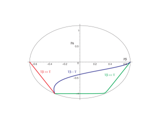
Figure 4: Transformed $SU(2)$ ellipse behaviour for $T_{\beta}\gg T$, $T_{\beta}\sim T$, $T_{\beta}\ll T$, plotted on the $(-)$ branch. The trajectories begin at the lower left as $t-t_{0}\rightarrow-\infty$, and evolve to the upper right as $t-t_{0}\rightarrow 0$.

Moreover, in Fig. 5 we plot the $T_{\beta}\ll T$ field behaviour of $z,\chi$, such that the $z$ displacement occurs in the reliable $\epsilon_{k}\ll 1$ regime after the change in $\chi$. Crucially, this means that the brane motion can occur in a $\epsilon_{k}\ll 1$ region without requiring $d>1$. Such behaviour could never have occurred in the original $SU(2)$ model, and is a consequence of the manner in which the fields $z$ and $\chi$ are incorporated together into a new, global structure for the overall solutions.

Figure 5: In the left hand plot we see $\phi$ and the $SU(2)$-transformed solution for $\beta$, with the remaining curve corresponding to the original untransformed $SU(2)$ solution for $\beta$. In the right hand plot we see the distinct $z$ and $\chi$ displacements, with the motion of the bulk brane $z$ occurring second. This allows the brane to displace with $d<1$ and yet still be in a $\epsilon_{k}\ll 1$ regime.

The fact that the displacement of $z$ can be made to entirely occur in a $\epsilon_{k}\ll 1$ regime, without requiring $d\gg 1$, constitutes a significant improvement over the original $SU(2)$ model. This proves that a reliable solution for $z$ does not necessarily require it to eventually leave the compact space . However, there are obviously other possible examples beyond those shown in Figs. 4-5, and we should now clarify the precise circumstances in which the $\epsilon_{k}$ can be made to decrease. Once again we consider the functional form of $\exp(\beta-\phi)$:

$$~{}e^{\beta-\phi}=\frac{3}{2qd^{2}}\left|\frac{t-t_{0}}{T}\right|^{\delta}\cdot\frac{\left(1+\left|\frac{t-t_{0}}{T}\right|^{-\tilde{\delta}}\right)^{2}}{\left|\frac{t-t_{0}}{T_{\beta}}\right|^{\delta-\tilde{\delta}}\left[1+\left|\frac{t-t_{0}}{T_{\beta}}\right|^{\delta_{\beta}}\left(1+\left|\frac{t-t_{0}}{T}\right|^{-\tilde{\delta}}\right)\right]}$$ (68)

By choosing signs appropriately, either the early or the late time limit can become “weakly-coupled” with $\epsilon_{k}\ll 1$. However, only one of the asymptotic limits can be weakly-coupled, with the other still becoming “strongly-coupled” with $\epsilon_{k}\gg 1$. There are, of course, still solutions where $\epsilon_{k}\gg 1$ is attained in both limits. The full state of affairs is summarised in table 2.

$s=+1$	$s=-1$	$s=-1$
$\delta,\delta_{\beta}<0$ on $(+)$	$\delta,\delta_{\beta}<0$ on $(+)$	$\delta+\delta_{\beta}<0,\delta_{\beta}<0,\delta>0$ on $(+)$
$\delta,\delta_{\beta}>0$ on $(-)$	$\delta,\delta_{\beta}>0$ on $(-)$	$\delta+\delta_{\beta}>0,\delta_{\beta}>0,\delta<0$ on $(-)$
SW	SS	WS

Table 2: Table to show the asymptotic values of the coupling parameters $\epsilon_{k}$, depending on the sign of $s$. The notation is as follows: strong-strong (SS), strong-weak (SW) and weak-strong (WS), where the first word corresponds to the $\epsilon_{k}$ values in the early-time limit, and the second refers to their values in the late-time limit.

Thus, there are three distinct types of solutions: weak-strong (WS), strong-weak (SW) and strong-strong (SS). In all three cases we can arrange for the $z$ motion to occur in a $\epsilon_{k}\ll 1$ region with $d<1$. To do this, we simply recognise that at $t-t_{0}\approx T$ we can always take $T_{\beta}\ll T$, and this will decrease the values of the $\epsilon_{k}$ below 1 without requiring $d\gg 1$. Consequently, there is a tremendous degree of flexibility in the solutions, and cases with $\epsilon_{k}\ll 1$ and $d<1$ are quite generic.

Before leaving this section, we should also comment on stringy $\alpha^{\prime}$ corrections. These become strong as we probe small length scales at $\beta\sim 0$, and so encounter new physics not accounted for in the effective supergravity description. As such, one must always ensure that $\beta\gg 0$ to trust any supergravity solution. We note that this is always possible for certain periods of time by an appropriate choice of integration constants, and so there is no obstruction to finding regimes where $\epsilon_{k}\ll 1$ and $\alpha^{\prime}$ corrections are extremely small. The transformed $SU(2)$ solutions thus incorporate all of the $z$ behaviour from the $SU(2)$ model, but now allow it to be compressed inside of the orbifold interval whilst simultaneously suppressing all unwanted corrections.

VIII Transforming the $SU(3)$ Toda model

We now apply the symmetries $L^{i}$ to the $SU(3)$ solutions, and so find a further class of new solutions. One finds in this case that only the action of the $L^{2}$ transformation can ever lead to new behaviour. This can be easily understood by noting that all the other transformations leave the $SU(3)$ truncation conditions Eq. (32) invariant, while $L^{2}$ allows $\dot{\nu}-\chi\dot{z}$ to become non-zero. The “activation” of this combination takes us outside of the original $SU(3)$ Toda model, and into a new situation that is not itself solvable by Toda methods. Nonetheless, the symmetries allow us to access an exact, analytical description of the behaviour when this combination is non-zero. We will find that the brane can undergo two displacements in opposite directions, and so reverse direction without the presence of any explicit potentials. We will often call this a “bouncing” solution.

VIII.1 Transformed-$SU(3)$ Solutions

These new solutions, although exact, are complicated and difficult to present in an elegant fashion. One means of presentation is to utilise two time-dependent functions $p,r$ that are implicitly defined via the relations

$$4r(4+p^{2})^{-1}=e^{\beta}|_{SU(3)}\quad,\quad pr(4+p^{2})^{-1}=\chi|_{SU(3)}$$ (69)

These are built out of the $\beta,\chi$ solutions from the old (untransformed) $SU(3)$ model. The new transformed-$SU(3)$ solutions can then be written in the form

$$\alpha=\alpha|_{SU(3)}\quad,\quad\phi=\phi|_{SU(3)}\quad,\quad\nu=\nu|_{SU(3)}$$

$$\beta=\ln\left\{4r\left[4+\left(p+c_{2}r\right)^{2}\right]^{-1}\right\}\quad,\quad\chi=r\left(p+c_{2}r\right)\left[4+\left(p+c_{2}r\right)^{2}\right]^{-1}\quad,\quad z=z|_{SU(3)}+c_{2}\nu|_{SU(3)}$$ (70)

Here $c_{2}$ is the real constant associated to the $L^{2}$ symmetry, and so corresponds to a new integration constant that can be varied at will. The remaining constants, it should be emphasised, are taken from the original $SU(3)$ model, and we should treat their values as determining an embedding of the old $SU(3)$ behaviour inside the newly transformed solutions. Indeed, the fields $\alpha,\phi,\nu$ are unaffected by the transformations, and evolve as in the old $SU(3)$ case in any event.

Notice as well that we cannot present $\sigma$ analytically, due to the fact that the corresponding $SU(3)$ solution can only be computed numerically. As such, the transformed $\sigma$ solution must also be computed numerically. However, we emphasise that these numerical computations can be readily carried out with no obstruction, and that the symmetry transformations induce perfectly sensible behaviour for $\sigma$ in all cases. In addition, $\sigma$ can have no bearing on the time-development of the other fields, as the condition $\dot{\sigma}+4qz\dot{\nu}=0$ is preserved under the symmetry group Eq. (54). This means that $\sigma$ never appears in the equations of motion of the other fields, and so can never induce any changes to the brane or remaining axions. Consequently, we will not particularly concern ourselves with $\sigma$ from this point on.

Having derived these new solutions by applying the symmetries, we must now consider the ramifications for the various fields involved. In particular, we are most interested in the field $z$ and the issue of whether we can now achieve a sensible displacement at weak-coupling. In the original $SU(3)$ model the field $z$ could undergo two successive displacements in the same direction, but it could not do so whilst entirely within a $\epsilon_{k}\ll 1$ regime. In the above case, however, the new field $z$ is an additive mixture of the old $SU(3)$ behaviours for $z,\nu$. This creates a significant new level of flexibility, and in the next section we will investigate the consequences for the brane and its displacements.

VIII.2 Analysis and Validity of the Transformed-$SU(3)$ model

Due to the complexity of the solutions, the field behaviour is somewhat difficult to determine by mere inspection. However, one can verify that the symmetry-transformation does not affect the asymptotic development, and so the same set of states are accessed on the ellipse at early and late time as in the $SU(3)$ model. However, the intermediate evolution is substantially, and interestingly, different. In Fig. 6 we plot some examples on the ellipse.

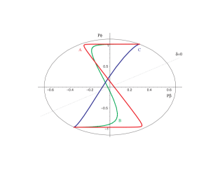
Figure 6: Here we show some examples of the transformed-$SU(3)$ solutions. Curve A is the original $SU(3)$ solution, and this can be progressively shifted toward curve B and into curve C as we change the integration constants.

The particularly interesting feature of these new solutions is the motion of the brane. Specifically, for certain special choices of constants, the brane can “bounce” and spontaneously reverse direction midway through its evolution. Moreover, a thorough investigation of the parameter space reveals that it is possible to make $\epsilon_{k}\ll 1$ whilst $z$ is undergoing this bounce strictly inside the orbifold interval. This is shown in Fig. 7.

Figure 7: The plot shows the transformed evolution of the brane $z$, and the parameters $\epsilon_{k}\propto\exp\left(\beta-\phi\right)$. Notice that the latter satisfy $\epsilon_{k}\ll 1$ while the brane is evolving, and that the brane reverses direction whilst still strictly inside the orbifold interval.

To see that this behaviour is indeed a consequence of the solutions in Eq. (70), one can proceed in the following qualitative fashion. First, we recognise that the effect of the symmetry transformation is to switch-on the combination $\dot{\nu}-\chi\dot{z}$ to a non-zero value. This then acts as a driving force that modifies the original $SU(3)$ evolution of $z$. Secondly, we recognise that this “modification”, at a practical level, amounts to additively mixing the $SU(3)$ behaviours of $z$ and $\nu$ together (see Eq. (VI)). So not only is $z$ affected, but it is affected by a non-trivial mixing together with the behaviour of $\nu$. Thirdly, the original $SU(3)$ field $\nu$ can already be made to reverse direction for particular choices of constants (see Eq. (48)). Hence, once mixed, the transformed $z$ solution also inherits this bouncing behaviour.

As before, this behaviour is subject to $\alpha^{\prime}$ corrections. However, the strength of these corrections can always be adjusted such that, when the brane is bouncing, the corrections are extremely small and so under control. Of course, the corrections cannot be made arbitrarily small for all time, but they can always be made arbitrarily small over significant periods of time when the brane is moving. To achieve this one simply tunes $c_{2}\ll 1$, which has the effect of setting $\beta\gg 0$ in the vicinity of the bounce.

These bouncing solutions richly extend the results of the previous sections. We now see that the effective supergravity action Eq. (1) admits exact solutions where the brane evolves in a regime with $\epsilon_{k}\ll 1$, has small $\alpha^{\prime}$ corrections, is strictly between the boundaries, and can also reverse direction mid-course. These effects were not at all obvious from the exactly integrable $SU(2)$ and $SU(3)$ Toda models, and yet can be generated by judiciously applying symmetries of the equations of motion. We also reiterate that no explicit potential was required to induce these effects; the reversal is a natural outcome of the non-linearly coupled cosmology.

IX Perturbations

In the previous section we presented several new classes of cosmological solution to heterotic M-theory, and found that the four-dimensional scale-factor $a=\exp\left({\alpha}\right)$ always satisfies $a\sim|t-t_{0}|^{1/3}$. Switching to conformal time $\eta$ defined by $d\eta=a^{-1}dt$, this translates into $a\sim|\eta-\eta_{0}|^{1/2}$. This means that on the $(+)$ branch we always have an expanding, decelerating universe, whilst on the $(-)$ branch we always have a contracting, inflationary universe. This behaviour is to be expected, for the cosmology we are studying has no explicit potentials and so $a$ remains unaffected by the other fields. We will now consider in more detail the inflationary epoch and the generation of perturbations on the $(-)$ branch.

As with the familiar PBB scenarios, the inflationary period on the $(-)$ branch is characterised by a comoving Hubble length $|d(\ln a)/d\eta|^{-1}=2|\eta-\eta_{0}|$ that decreases as we take $\eta\rightarrow\eta_{0}$ and approach the Big Bang singularity from below. Consequently, a given comoving scale starting inside the Hubble radius as $\eta\rightarrow-\infty$ automatically becomes larger than the Hubble radius as $\eta\rightarrow\eta_{0}$. Therefore, on the $(-)$ branch one can produce super-horizon scale perturbations merely from kinetic-driven inflation, without the use of any potentials. This is considered an interesting alternative to conventional inflation on the $(+)$ branch, since PBB scenarios do not require special choices of potential or slow-roll conditions. Given this, it is interesting to consider the perturbation spectra of our fields on the $(-)$ branch, and see whether there any useful scale-invariant modes. Not surprisingly, we will be able to utilise the techniques developed in PBB cosmology to aid our calculations. We will also see that the factor of $3$ in the kinetic terms for $\beta$ and $\chi$, which complicated the classification of the scalar-field manifold (see Ref. Copeland:2005mk ) has interesting consequences for the spectral indices of the fields.

We will begin by considering perturbations around a special background where the axions $\chi,\sigma,\nu$ have been set to constants, and where the conserved quantity in Eq. (15) has been set to zero. In this case the brane $z$ remains static for all time, and entirely decouples from the equations of motion of $\beta$ and $\phi$. The fields $\beta,\phi$ then exhibit standard rolling-radii behaviour with unrestricted parameters, and no transitions on the ellipse occur. Although this special “vacuum” situation does not incorporate any interesting brane displacements in the background, it proves to be a much simpler situation that can be solved analytically. Later, we will comment on perturbations around more general backgrounds, including the various Toda models and their symmetry transforms. In the meantime, we note that in the simple vacuum case the $\beta$ and $\phi$ perturbations remain coupled to the metric perturbations, and produce adiabatic perturbations with the same steep $n=4$ blue spectra that occurs in PBB cosmology Lidsey:1999mc ; Brustein:1994kn . In contrast, the fields $z,\sigma,\chi,\nu$ with constant background values are decoupled from the metric perturbations, and produce isocurvature perturbations $\delta z,\delta\sigma,\delta\chi,\delta\nu$ with different spectra.

The first-order, gauge-invariant perturbation equations for $\delta z,\delta\sigma,\delta\chi,\delta\nu$ in conformal time are given by

$$\delta z^{\prime\prime}+(2\alpha^{\prime}+\beta^{\prime}-\phi^{\prime})\delta z^{\prime}+k^{2}\delta z =0$$

$$\delta\sigma^{\prime\prime}+2(\alpha^{\prime}-\phi^{\prime})\delta\sigma^{\prime}+k^{2}\delta\sigma =-4qz(\beta^{\prime}-\phi^{\prime})\delta\nu^{\prime}+8qz\chi\beta^{\prime}\delta z^{\prime}$$ (71)

$$\delta\chi^{\prime\prime}+2(\alpha^{\prime}-\beta^{\prime})\delta\chi^{\prime}+k^{2}\delta\chi =0$$

$$\delta\nu^{\prime\prime}+(2\alpha^{\prime}-\beta^{\prime}-\phi^{\prime})\delta\nu^{\prime}+k^{2}\delta\nu =-2\chi\beta^{\prime}\delta z^{\prime}.$$ (72)

Here a $\prime$ denotes a derivative with respect to $\eta$, and $k$ is the comoving wavenumber of the perturbation. In order to solve for these four isocurvature perturbations we will use techniques familiar from the PBB literature, with $z$ replacing an axion. This involves making an appropriate conformal transformation on the metric into each axion’s frame so as to eliminate the coupling to $\beta,\phi$, and then solving the resulting perturbation equations in the usual manner (see Refs. Lidsey:1999mc ; Copeland:1998ie ; Copeland:1997ug ). However, before we do this we need to deal with the awkward source terms on the right-hand sides of Eq. (71) and Eq. (72). The presence of the bulk-brane field $z$ on the right-hand side of Eq. (71), rather than a true axion, slightly complicates the situation as we cannot simply set $z=0$ as we can with $\chi$ in Eq. (72). Recall that our theory is only valid when $z\in(0,1)$. Instead, we must deal with the source terms by choosing appropriate combinations of perturbations: $\delta A=\delta\sigma+4qz\delta\nu$ and $\delta B=\delta\nu-\chi\delta z$ .

Following the calculations of Ref. Copeland:1998ie , we can now define a new metric for each field’s frame by making a conformal transformation on the Einstein metric: $\bar{g}_{j\;\mu\nu}=\Omega_{j}^{2}g_{\mu\nu}$. Our conformal factors $\Omega_{j}$ are explicitly given by

$$\Omega_{z}^{2}=e^{\beta-\phi}\,,\quad\Omega_{A}^{2}=e^{-2\phi}\,,\quad\Omega_{\chi}^{2}=e^{-2\beta}\,,\quad\Omega_{B}^{2}=e^{-\beta-\phi}$$ (73)

These conformal transformations lead to a different scale factor $\bar{a}_{j}=\Omega_{j}a$ in each frame, depending on each fields coupling to $\beta,\phi$. As we are considering static axions and bulk brane, $\beta,\phi$ behave as simple rolling-radii fields with fixed parameters that lie at one point on the ellipse, Eq. (22), for all time. Explicitly, in conformal time they satisfy

$$a=a_{*}|\eta|^{\frac{1}{2}}\quad,\quad\beta=\frac{3}{2}p_{\beta}\ln|\eta|+\beta_{0}\quad,\quad\phi=\frac{3}{2}p_{\phi}\ln|\eta|+\phi_{0}$$ (74)

where $a_{*}$ is a constant, and we have conveniently set $\eta_{0}=0$. Using these background solutions one can show that

$$\bar{a}_{j}=\bar{a}_{*j}|\eta|^{\frac{1}{2}+r_{j}}\quad{\rm with}\quad r_{z}=\frac{3}{4}(p_{\beta}-p_{\phi})\,,\quad r_{A}=-\frac{3}{2}p_{\phi}\,,\quad r_{\chi}=-\frac{3}{2}p_{\beta}\,,\quad r_{B}=-\frac{3}{4}(p_{\beta}+p_{\phi})$$ (75)

where the $\bar{a}_{*j}$ are a set of constants. In these new frames we then find that the perturbation equations can be recast in the form

$$\delta x_{j}^{\prime\prime}+2\bar{\alpha}_{j}^{\prime}\delta x_{j}^{\prime}+k^{2}\delta x_{j}=0$$

where $\delta x_{j}=(\delta z,\delta A,\delta\chi,\delta B)$ and $\bar{\alpha}_{j}^{\prime}=\bar{a}_{j}^{\prime}/\bar{a}_{j}$ is the Hubble rate in each conformal frame. The solution for our isocurvature perturbations, after normalising at early time, is then given by (see Ref. Copeland:1998ie )

$$\delta x_{j}=\kappa\sqrt{\frac{\pi}{m_{j}k}}\exp\left[\frac{i\pi}{4}\left(1+2|r_{j}|\right)\right]\frac{(-k\eta)^{1/2}}{\bar{a}_{j}}H_{|r_{j}|}^{(1)}(-k\eta)$$

Here the $m_{j}$ are given by $m_{z}=2q$, $m_{A}=4$, $m_{\chi}=12$, $m_{B}=8q$, and $H_{J}^{(1)}$ is the Hankel function of the first kind and order $J$. Defining the power spectrum $P_{\delta x}$ and its spectral index $n_{\delta x}$ for a general perturbation $\delta x$ as

$$P_{\delta x}=\frac{k^{3}}{2\pi^{2}}|\delta x|^{2}\quad{\rm and}\quad n_{\delta x}-1=\frac{d\ln P_{\delta x}}{d\ln k}$$

we find the spectral index for each of the isocurvature perturbations is given by

$$n_{\delta x_{j}}=4-2|r_{j}|$$

Looking at the definitions of the $|r_{j}|$ given in Eq. (75), we see how the spectral indices are dependent on the coupling of $z$ and the axions to $\phi,\beta$ and consequently their expansion powers, $p_{\phi}$ and $p_{\beta}$. Inserting the specific couplings for each field and considering the range of background solutions yields

$$n_{\delta A}=4-3|p_{\phi}|\,:\quad\in[4-2\sqrt{3},4]\quad\sim\quad[0.54,4],$$

$$n_{\delta z}=4-\frac{3}{2}|(p_{\beta}-p_{\phi})|\,,\quad n_{\delta\chi}=4-3|p_{\beta}|\,,\quad n_{\delta B}=4-\frac{3}{2}|(p_{\beta}+p_{\phi})|\,:\quad\in[2,4]$$

Thus we find that our perturbation $\delta A$ has the classic axion perturbation spectrum familiar from PBB calculations, and can provide a scale-invariant spectrum. In contrast, the bulk brane and other axion perturbations cannot provide a scale-invariant spectrum, a result similar to the one obtained in Ref. DiMarco:2002eb .

One can also write the spectral indices as a function of a single variable by using the ellipse constraint, Eq. (22). This reveals

$$n_{\delta z}=4-\left|\pm\sqrt{4-3p_{\phi}^{2}}-3p_{\phi}\right|\,,\quad n_{\delta A}=4-3|p_{\phi}|\,,\quad$$

$$n_{\delta\chi}=4-\sqrt{4-3p_{\phi}^{2}}\,,\quad n_{\delta B}=4-\left|\pm\sqrt{4-3p_{\phi}^{2}}+3p_{\phi}\right|$$

where $p_{\phi}\in[-2/\sqrt{3},2/\sqrt{3}]$ for the vacuum case. One should remember that the choice of $\pm$ sign must be consistently applied across all the spectral indices, and that both signs are always valid choices (as we do not have to satisfy $p_{\beta}-p_{\phi}>0$ in the vacuum case).

If one is familiar with PBB calculations the above result may be surprising, as axion perturbations derived from actions very similar to ours will usually all have spectral indices in the range $[4-2\sqrt{3},4]$. (See, for example, the variety of dilaton-moduli-axion systems discussed in Refs. Lidsey:1999mc ; Copeland:1998ie ; Copeland:1997ug ; Bridgman:2000kk ). This change is a direct consequence of the coupling of our fields to $\beta$, which unlike in PBB cosmology has a factor of $3$ in its kinetic term. This then affects the range of $p_{\beta}$ through the ellipse condition. One cannot change this result by rescaling $\beta$’s kinetic term as this rescales $\beta$’s coupling to the fields and moves the effect into the $r_{j}$ definitions. This then leaves $\delta A$ as the single perturbation capable of producing a scale-invariant spectrum.

So far we have only been considering the “vacuum” solutions where $z$ and the axions remain constant. However, generalising these solutions to the case with moving brane and axions remains an open question, due to the sheer complexity of the solutions considered. One can begin by truncating off the axions and considering the perturbations of the $\phi,\beta,z$ $SU(2)$ action of Section IV. In this case one can use an $SL(2,\mathbb{R})$ symmetry of the truncated action  to solve for the perturbation $\delta z$ around a moving-brane $SU(2)$ background, by applying the $SL(2,\mathbb{R})$ symmetry to perturbations $\delta\phi,\delta\beta,\delta z$ around a static-brane $SU(2)$ background. One then finds that this “rotated” $\delta z$ isocurvature perturbation retains the spectrum $n\in[2,4]$  (see Ref. DiMarco:2002eb ). However, the effect of this rotation on the remaining axionic equations leaves a non-trivial calculation.

As a result, we can only conjecture that a scale-invariant mode persists in perturbations around the Toda model backgrounds and their symmetry transforms. However, it is certainly true that all of the solutions we have considered will asymptotically approach the “vacuum” scenario. Moreover, when one applies the constraints on $p_{\phi}$ in the various classes of solutions one finds that, in a least one of the asymptotic limits, the rolling-radii regime which leads to $\delta A$ producing a scale-invariant spectrum is accessible. Hence, we can always generate a scale-invariant mode in one of the asymptotic limits, even if we cannot determine whether such a mode can also be generated at intermediate times.

X Conclusion

We have presented several new classes of cosmological solution to the four-dimensional effective supergravity description of heterotic M-theory. This theory contain seven fields: the four-dimensional scale-factor $\alpha$, the modulus $\beta$ measuring the separation of the orbifold planes, the axion $\chi$ related to the graviphoton field, the dilaton $\phi$ measuring the average Calabi-Yau volume, the axion $\sigma$ related to the bulk three-form, the field $z$ locating the position of the M5 brane, and the axion $\nu$ representing the self-dual two-form on the brane worldvolume. To linear-order in the moduli-dependent parameters $\epsilon_{k}$ $(k=1,2)$, all fields except $\alpha$ can be described by the following scalar-field Lagrangian

$$\mathcal{L}=\frac{3}{4}(\partial\beta)^{2}+3e^{-2\beta}(\partial\chi)^{2}+\frac{1}{4}(\partial\phi)^{2}+\frac{1}{4}e^{-2\phi}\left(\partial\sigma+4qz\partial\nu\right)^{2}+\frac{1}{2}qe^{\beta-\phi}(\partial z)^{2}+2qe^{-\beta-\phi}(\partial\nu-\chi\partial z)^{2}$$

We have attempted to identify as many exact solutions to this system as possible, by identifying special constraints on the fields that simplify the analysis. The only previously known solution to this Lagrangian, as described in Ref. Copeland:2001zp , is found when $\mathcal{L}$ is consistently truncated to the form

$$\mathcal{L}_{SU(2)}=\frac{3}{4}(\partial\beta)^{2}+\frac{1}{4}(\partial\phi)^{2}+\frac{1}{2}qe^{\beta-\phi}(\partial z)^{2}$$

The fields $\beta,\phi,z$ then form an exactly-solvable $SU(2)$ Toda model, with the brane $z$ undergoing single displacements. In this paper we have identified three new solutions in addition to this $SU(2)$ Toda solution. The first new solution was found by consistently truncating $\mathcal{L}$ to the different form

$$\mathcal{L}_{SU(3)}=\frac{3}{4}(\partial\beta)^{2}+3e^{-2\beta}(\partial\chi)^{2}+\frac{1}{4}(\partial\phi)^{2}+\frac{1}{2}qe^{\beta-\phi}(\partial z)^{2}$$

using the conditions $\partial\nu-\chi\partial z=\partial\sigma+4qz\partial\nu=0$. By switching off these two terms, one finds that the reduced set of fields $\beta,\chi,\phi,z$ span an integrable $SU(3)$ Toda model, and can be solved for exactly. This $SU(3)$ model allows for double displacements of the brane $z$, and the $SU(3)$ solutions can always be made reliable with $\epsilon_{k}\ll 1$ over a certain period of time during this double displacement. However, the brane must leave the compact space in any solution that has reliable $\epsilon_{k}\ll 1$ regime at some point.

Next, we applied to the $SU(2)$ and $SU(3)$ models the symmetry transformations derived and discussed in our companion Ref. Copeland:2005mk . This enabled us to derive two new and distinct cosmological solutions. The properties of these new solutions were then discussed at length, and it was found that the reliability of the solutions had been radically affected. This is ultimately due to the $SL(2,\mathbb{R})$ subgroup of symmetries, which acts as a “generalised” set of $T$-duality transformations given by

$$T^{\prime}=\frac{aT-ib}{icT+d}\quad,\quad Z^{\prime}=\frac{Z}{icT+d}\quad,\quad S^{\prime}=S-\frac{icqZ^{2}}{icT+1}\quad\mathrm{with}\quad a,b,c,d\in\mathbb{R}\quad,\quad ad-bc=1$$ (76)

This is not ordinary $T$-duality, as all three complex fields $T,S,Z$ are affected. Using these symmetries, it was then found in the $SU(2)$-transformed solutions that the brane can undergo a single displacement entirely within the orbifold interval with $\epsilon_{k}\ll 1$ throughout. It was also found in the $SU(3)$-transformed solutions that the brane field $z$ can undergo two successive displacements of opposite sign and so reverse direction. The specific conditions under which this reversal occurs are as follows. Firstly, set $\partial\sigma+4qz\partial\nu=0$ so that the axion $\sigma$ is decoupled from the other fields. Then the scalar-field lagrangian $\mathcal{L}$ reduces to the simpler form

$$\mathcal{L^{\prime}}=\frac{3}{4}(\partial\beta)^{2}+3e^{-2\beta}(\partial\chi)^{2}+\frac{1}{4}(\partial\phi)^{2}+\frac{1}{2}qe^{\beta-\phi}(\partial z)^{2}+2qe^{-\beta-\phi}(\partial\nu-\chi\partial z)^{2}$$

One then proceeds by setting $\partial\nu-\chi\partial z=0$ and solving the system as an $SU(3)$ Toda model, but then restoring the $\partial\nu-\chi\partial z$ term to a general, non-zero value by applying an $SL(2,\mathbb{R})$ symmetry. In particular, the fields $z,\nu$ transform as a doublet under $SL(2,\mathbb{R})$, and so we can solve the system with general $\partial\nu-\chi\partial z$ by “rotating” from a solution where it is zero. As a consequence, the equations of motion arising from the reduced lagrangian $\mathcal{L^{\prime}}$ have been completely solved in this paper. Further, by tuning the sign and magnitude of the $-\chi\partial z$ contribution generated by the symmetry application, one can modify the overall velocity of the brane so that it comes to rest and reverses direction. This is a particularly interesting feature arising from the coupling with $\chi$, whose presence in the kinetic term $\partial\nu-\chi\partial z$ is due to the need for a gauge-covariant derivative in five dimensions. This reversing behaviour, which we have occasionally called a “bouncing” solution, can also be made to occur entirely within the orbifold interval with $\epsilon_{k}\ll 1$ throughout.

As such, all of the transformed solutions demonstrate a rich new variety of M5 brane behaviours, and new, trustworthy regions of solution space emerge that had not previously been identified. In particular, we conjecture that reversing brane solutions will exist in other corners of string theory beyond heterotic M-theory. One can pin down reasonably clear “minimum conditions” for this reversal to occur, as follows. Firstly, at least one modulus should be active, such as the dilaton $\phi$, whose coupling to the brane kinetic term will induce the brane $z$ to undergo a single displacement. Secondly, there should also be an active combination proportional to a cross-coupling between an axion field and $\partial z$. This second combination can then be adjusted so that the brane turns around at some point during its motion.

As an interesting corollary, we then considered the isocurvature perturbation spectra produced by the model in an inflationary contracting (PBB) phase. In the “vacuum” case we found that one of the isocurvature modes – the one associated with the axions $\sigma$ and $\nu$ – is able to produce a scale-invariant spectrum. Furthermore, we found that all of the solutions considered will asymptotically approach this vacuum case in at least one asymptotic limit, and so a scale-invariant perturbation spectrum can always be generated asymptotically when perturbing around any of the solutions we have studied. However, the detailed structure of the perturbation spectrum at intermediate times has not yet been computed in its full generality, and it would be interesting to study this problem in greater depth, perhaps in a manner analogous to the numerical approach developed in Refs. Cartier:2003jz ; Cartier:2004zn .

Finally, we note that the methodologies employed in this paper have much wider applicability. For example, the Toda model solution method, as extensively detailed in Refs. Kostant:1979qu ; Lukas:1996iq , is not restricted to scalar-field systems arising from heterotic M-theory, and could be readily utilised in other areas of string theory. Likewise, it is equally plausible that other braneworld Kähler metrics may possess useful symmetry groups, which can be used to transform subsystems of fields into new patterns of behaviour. In light of this, it would be interesting to clarify the origin of the special $SL(2,\mathbb{R})$ symmetry group that we have found, and understand the general conditions under which reversing brane behaviour occurs in string and M-theory.

Appendix A

In this Appendix we present certain additional details of the $SU(3)$ Toda model derivation. We do this because the derivation is rather complicated, particularly the manner in which one must change time-gauges and judiciously redefine constants.

To begin with, we know that the vectors $\mathbf{q}_{1},\mathbf{q}_{2}$ are proportional to the two simple root-vectors of $SU(3)$. Utilising this fact, we can choose a basis for the space $(\alpha,\beta,\phi)$ that is adapted to the underlying $SU(3)$ symmetry, and so consists of vectors $\mathbf{e}_{0},\mathbf{e}_{1},\mathbf{e}_{2}$ satisfying

$$<\mathbf{e}_{0},\mathbf{e}_{0}>=-1\quad,\quad<\mathbf{e}_{0},\mathbf{e}_{1}>\>=\><\mathbf{e}_{0},\mathbf{e}_{2}>\>=\>0\quad,\quad\mathbf{e}_{1}=\frac{3}{8}\mathbf{q}_{1}\quad,\quad\mathbf{e}_{2}=\frac{3}{8}\mathbf{q}_{2}$$ (77)

A choice of basis compatible with these conditions is given by

$$\mathbf{e}_{0}=(\sqrt{3},0,0)\quad,\quad\mathbf{e}_{1}=\frac{3}{8}(0,-1,1)\quad,\quad\mathbf{e}_{2}=\frac{3}{8}(0,2,0)$$ (78)

We now write the covariant vector $G\mbox{\boldmath$\alpha$}$ as the following sum

$$G\mbox{\boldmath$\alpha$}=\sum_{i=0}^{2}\rho_{i}(\tau)\mathbf{e}_{i}$$ (79)

and insert this time-dependent expansion into the equations of motion to find the evolution of the “modes” $\rho_{i}$. Choosing the convenient gauge $n=3\alpha$ (or $E=1$) one finds

$$\ddot{\rho}_{0}=0$$ (80)

$$\ddot{\rho}_{1}+\frac{4}{3}u_{1}^{2}e^{2\rho_{1}-\rho_{2}}=0$$ (81)

$$\ddot{\rho}_{2}+\frac{4}{3}u_{2}^{2}e^{2\rho_{2}-\rho_{1}}=0$$ (82)

$$-\dot{\rho}_{0}^{2}+\frac{3}{4}\left(\dot{\rho}_{1}^{2}-\dot{\rho}_{1}\dot{\rho}_{2}+\dot{\rho}_{2}^{2}\right)+2U=0$$ (83)

The general solution to these equations is now easy to come by, and takes the form

$$\rho_{0} =-k_{0}(\tau-\tau_{0})$$ (84)

$$\rho_{1} =-\ln{g_{1}(\tau)}$$ (85)

$$\rho_{2} =-\ln{g_{2}(\tau)}$$ (86)

where $k_{0},\tau_{0}$ are constants. The functions $g_{1},g_{2}$ are given by a sum over the collection of weight vectors $\mbox{\boldmath$\Lambda$}_{1}=\{(0,-1),(-1,1),(1,0)\}$, $\mbox{\boldmath$\Lambda$}_{2}=\{(-1,0),(1,-1),(0,1)\}$ of the fundamental $\mathbf{3}$ and $\bar{\mathbf{3}}$ representations of $SU(3)$. Concretely, if we define the matrix of vectors

$$\mbox{\boldmath$\lambda$}_{ij}=\left(\begin{array}[]{c}\mbox{\boldmath$\Lambda$}_{1}\\ \mbox{\boldmath$\Lambda$}_{2}\end{array}\right)=\left(\begin{array}[]{ccc}(0,-1)&(-1,1)&(1,0)\\ (-1,0)&(1,-1)&(0,1)\end{array}\right)$$ (91)

then for $i=1,2$ the functions $g_{i}$ are given by

$$g_{i}=\sum_{j=1}^{3}a_{ij}\>\mathrm{exp}\left[\mbox{\boldmath$\lambda$}_{ij}\cdot\left(\mathbf{k}\tau-\mbox{\boldmath$\tau$}\right)\right]$$ (92)

where the positive constants $a_{ij}$ are

$$a_{11} =\frac{4u_{2}^{2}}{3}\left(\frac{2k_{1}-k_{2}}{P}\right) a_{21} =\frac{4u_{2}^{2}}{3}\left(\frac{2k_{2}-k_{1}}{P}\right)$$

$$a_{12} =\frac{4u_{1}^{2}}{3}\left(\frac{k_{1}+k_{2}}{P}\right) a_{22} =\frac{4u_{2}^{2}}{3}\left(\frac{k_{1}+k_{2}}{P}\right)$$

$$a_{13} =\frac{4u_{1}^{2}}{3}\left(\frac{2k_{2}-k_{1}}{P}\right) a_{23} =\frac{4u_{1}^{2}}{3}\left(\frac{2k_{1}-k_{2}}{P}\right)$$

and $P=(2k_{1}-k_{2})(2k_{2}-k_{1})(k_{1}+k_{2})$. The constant vector $\mbox{\boldmath$\tau$}=(\tau_{1},\tau_{2})$ is a set of arbitrary time-shifts. The constant vector $\mathbf{k}=(k_{1},k_{2})$ is restricted to the open Weyl chamber, which means it is forced to have positive scalar product with the two simple root-vectors as follows

$$(k_{1},k_{2})\cdot(2,-1) =2k_{1}-k_{2}>0$$

$$(k_{1},k_{2})\cdot(-1,2) =2k_{2}-k_{1}>0\;.$$ (93)

These two conditions guarantee that $g_{1},g_{2}>0$ so that the logarithms in $\rho_{1},\rho_{2}$ are always well-defined. Lastly, we must also impose the Friedmann constraint

$$-k_{0}^{2}+\frac{3}{4}\left(k_{1}^{2}-k_{1}k_{2}+k_{2}^{2}\right)=0\;.$$ (94)

Using the information above, one can arrive at an explicit solution for the fields $\alpha,\beta,\phi$ and the two additional fields $z,\chi$ that were integrated out. Recall that

$$\mbox{\boldmath$\alpha$}=\left(\begin{array}[]{c}\alpha\\ \beta\\ \phi\end{array}\right)=\sum_{i=0}^{2}\rho_{i}G^{-1}\mathbf{e}_{i}=\left(\begin{array}[]{c}-\frac{1}{\sqrt{3}}\rho_{0}\\ \rho_{2}-\frac{1}{2}\rho_{1}\\ \frac{3}{2}\rho_{1}\end{array}\right)$$ (101)

and that

$$g_{1}(\tau) =a_{11}e^{-k_{2}\tau+\tau_{2}}+a_{12}e^{(k_{2}-k_{1})\tau-(\tau_{2}-\tau_{1})}+a_{13}e^{k_{1}\tau-\tau_{1}}$$

$$g_{2}(\tau) =a_{21}e^{-k_{1}\tau+\tau_{1}}+a_{22}e^{(k_{1}-k_{2})\tau-(\tau_{1}-\tau_{2})}+a_{23}e^{k_{2}\tau-\tau_{2}}$$ (102)

Then we find

$$\alpha =\frac{1}{\sqrt{3}}\>k_{0}\left(\tau-\tau_{0}\right)$$ (103)

$$\beta =\frac{1}{2}\ln\left[a_{11}e^{-k_{2}\tau+\tau_{2}}+a_{12}e^{(k_{2}-k_{1})\tau-(\tau_{2}-\tau_{1})}+a_{13}e^{k_{1}\tau-\tau_{1}}\right]$$

$$\quad-\ln\left[a_{21}e^{-k_{1}\tau+\tau_{1}}+a_{22}e^{(k_{1}-k_{2})\tau-(\tau_{1}-\tau_{2})}+a_{23}e^{k_{2}\tau-\tau_{2}}\right]$$

$$\phi =-\frac{3}{2}\ln\left[a_{11}e^{-k_{2}\tau+\tau_{2}}+a_{12}e^{(k_{2}-k_{1})\tau-(\tau_{2}-\tau_{1})}+a_{13}e^{k_{1}\tau-\tau_{1}}\right]$$

$$z-z_{0} =C_{z}\frac{\dot{g_{1}}}{g_{1}}=C_{z}\left[\frac{-k_{2}a_{11}e^{-k_{2}\tau+\tau_{2}}+(k_{2}-k_{1})a_{12}e^{(k_{2}-k_{1})\tau-(\tau_{2}-\tau_{1})}+k_{1}a_{13}e^{k_{1}\tau-\tau_{1}}}{a_{11}e^{-k_{2}\tau+\tau_{2}}+a_{12}e^{(k_{2}-k_{1})\tau-(\tau_{2}-\tau_{1})}+a_{13}e^{k_{1}\tau-\tau_{1}}}\right]$$

$$\chi-\chi_{0} =C_{\chi}\frac{\dot{g_{2}}}{g_{2}}=C_{\chi}\left[\frac{-k_{1}a_{21}e^{-k_{1}\tau+\tau_{1}}+(k_{1}-k_{2})a_{22}e^{(k_{1}-k_{2})\tau-(\tau_{1}-\tau_{2})}k_{2}a_{23}e^{k_{2}\tau-\tau_{2}}}{a_{21}e^{-k_{1}\tau+\tau_{1}}+a_{22}e^{(k_{1}-k_{2})\tau-(\tau_{1}-\tau_{2})}+a_{23}e^{k_{2}\tau-\tau_{2}}}\right]$$

where $z_{0},\chi_{0}$ are constants of integration, and

$$C_{z}=\left(\frac{9}{8qu_{1}^{2}}\right)^{\frac{1}{2}}\quad,\quad C_{\chi}=\left(\frac{3}{16u_{2}^{2}}\right)^{\frac{1}{2}}$$

We can then deduce the forms of $\sigma,\nu$ that are compatible with the ancillary conditions Eq. (32)

$$\nu-\nu_{0} =\chi_{0}(z-z_{0})+C_{z}C_{\chi}\left[\frac{k_{2}(2k_{1}-k_{2})a_{13}e^{k_{1}\tau-\tau_{1}}+k_{1}(2k_{2}-k_{1})a_{23}e^{-k_{2}\tau+\tau_{2}}}{a_{11}e^{-k_{2}\tau+\tau_{2}}+a_{12}e^{(k_{2}-k_{1})\tau-(\tau_{2}-\tau_{1})}+a_{13}e^{k_{1}\tau-\tau_{1}}}\right]$$

$$\sigma-\sigma_{0} =-2q\left[2z_{0}\nu+\chi_{0}(z-z_{0})^{2}+\int\left[(z-z_{0})^{2}\right]^{\centerdot}(\chi-\chi_{0})d\tau\right]$$

where $\nu_{0},\sigma_{0}$ are two further constants of integration. Notice that the integral in the $\sigma$ solution is not elementary, and so cannot be written as a finite (potentially nested) sequence of logs, exponentials and rational functions of $\tau$. However, it can sometimes be analytically integrated for fixed choices of the arbitrary constants, and in any event has a sensible definite integral between fixed $\tau$ limits. In particular, one can compute the $\sigma$ behaviour numerically for any given set of starting conditions.

It is useful to understand the asymptotic limits, in order to transform these solutions to the proper time-gauge $n=0$. One finds that

$$e^{\beta} \sim e^{\left(2k_{1}-k_{2}\right)\tau/2}\quad\mathrm{and}\quad e^{\phi}\sim e^{3k_{2}\tau/2}\quad\mathrm{as}\quad\tau\rightarrow-\infty$$

$$e^{\beta} \sim e^{\left(k_{1}-2k_{2}\right)\tau/2}\quad\mathrm{and}\quad e^{\phi}\sim e^{-3k_{1}\tau/2}\quad\mathrm{as}\quad\tau\rightarrow+\infty$$

Since $2k_{1}-k_{2}>0$ and $k_{1}-2k_{2}<0$ we see that the orbifold radius $\beta$ always goes from a state of expansion at early time to a state of contraction at late time. The same is true of the modulus $\phi$ that measures the orbifold-averaged Calabi-Yau volume. These two fields will then have some complicated intermediate transition(s) that smoothly link these extreme limits. On the other hand, the fields $z$ and $\chi$ always asymptote to constants in the limits, although these constants are generally different. They too will undergo some intermediate “displacement” consistent with the different constant field values at early and late time.

We now change from logarithmic time $\tau$ to proper time $t$. Since the logarithmic-time gauge is given by $n=3\alpha$, we can find the relation to proper time by integrating the defining relation

$$dt\equiv e^{n(\tau)}d\tau=e^{3\alpha(\tau)}d\tau=e^{\sqrt{3}k_{0}(\tau-\tau_{0})}d\tau$$ (104)

This gives

$$\alpha=\frac{1}{3}\ln\left[\sqrt{3}k_{0}(t-t_{0})\right]\equiv\frac{1}{3}\ln\left|\frac{t-t_{0}}{T_{0}}\right|$$ (105)

where $t_{0}$ is a finite integration constant. This leads to two disconnected time branches corresponding to the choices $t-t_{0}>0,T_{0}>0$ and $t-t_{0}<0,T_{0}<0$, both of which lead to a well-defined positive argument for the logarithm. The regime $t-t_{0}>0,T_{0}>0$ will be referred to as the “positive-time” or simply $(+)$ branch, whilst the sector $t-t_{0}<0,T_{0}<0$ will be dubbed the “negative-time” or simply $(-)$ branch. The physics in the time interval $\tau\in(-\infty,+\infty)$ is mapped to these two regions in the following way. The early time $\tau\rightarrow-\infty$ regime with expanding $\beta,\phi$ corresponds to $t-t_{0}\rightarrow 0$ on the $(+)$ branch and $t-t_{0}\rightarrow-\infty$ on the $(-)$ branch, while the late time regime $\tau\rightarrow\infty$ corresponds to $t-t_{0}\rightarrow\infty$ on the $(+)$ branch and $t-t_{0}\rightarrow 0$ on the $(-)$ branch. It should be noted these two time branches in $t$ are physically separated by an unavoidable curvature singularity at $t=t_{0}$, despite the fact that in the $\tau$-gauge we had only one physical region. After this gauge change, typical terms in $\rho_{1},\rho_{2}$ will then scale as

$$\left|\frac{t-t_{0}}{T_{0}}\right|^{\lambda_{i}^{\prime}}\quad,\quad\left|\frac{t-t_{0}}{T_{0}}\right|^{-\lambda_{i}^{\prime}}$$

respectively, where $\lambda_{i}^{\prime}=(k^{\prime}_{1},k_{2}^{\prime}-k_{1}^{\prime},-k_{2}^{\prime})$ and

$$k_{1}^{\prime}=k_{1}T_{0}\quad,\quad k_{2}^{\prime}=k_{2}T_{0}$$

Note that $k_{1}^{\prime},k_{2}^{\prime}$ can be of either sign depending upon the sign of $T_{0}$ and so the choice of branch. On the positive branch we have $k_{1}^{\prime},k_{2}^{\prime}>0$ so that $k_{1}^{\prime}=|k_{1}^{\prime}|,k_{2}^{\prime}=|k_{2}^{\prime}|$. In this gauge the fields $\beta,\phi$ scale asymptotically at early-time as

$$\beta\sim p_{\beta,i}\ln|t-t_{0}|\quad,\quad\phi\sim p_{\phi,i}\ln|t-t_{0}|$$

where we have defined the two constants

$$p_{\beta,i}=\frac{1}{2}\left(2|k_{1}^{\prime}|-|k_{2}^{\prime}|\right)\quad,\quad p_{\phi,i}=\frac{3}{2}|k_{2}^{\prime}|$$

The Friedmann constraint Eq. (94) then reduces to the familiar ellipse condition

$$p_{\phi,i}^{2}+3p_{\beta,i}^{2}=\frac{4}{3}$$

Moreover, the Weyl chamber constraints $2|k_{1}^{\prime}|-|k_{2}^{\prime}|>0,\>2|k_{2}^{\prime}|-|k_{1}^{\prime}|>0$ translate into $p_{\beta,i}>0,\>\delta<0$. So the positive branch is associated to $\delta<0$ with the further additional constraint that $\delta_{\beta}=-2p_{\beta,i}<0$. Conversely, on the negative time branch we find the opposite results, since we follow the ellipse trajectories backward. Hence, we find that $\delta,\delta_{\beta}>0$.

Since all the fields involved are scalars, we are now free to substitute $\tau$ in terms of $t$ in all the solutions. These will then be the $n=0$ forms for the solutions. To make these solutions look “nice”, however, one must carefully redefine certain constants. If one defines new timescales $T,T_{\beta}$ via

$$\left|\frac{T}{T_{0}}\right|^{\delta}=\frac{a_{12}}{a_{11}}\exp\left[-(k_{1}-2k_{2})\tau_{0}+(\tau_{1}-2\tau_{2})\right]\quad,\quad\left|\frac{T_{\beta}}{T_{0}}\right|^{\delta_{\beta}}=\frac{a_{22}}{a_{21}}\exp\left[(2k_{1}-k_{2})\tau_{0}-(2\tau_{1}-\tau_{2})\right]$$

then the resulting solutions look relatively simple. They can be made even simpler by defining the ubiquitous fractional combinations

$$\theta_{z}=\frac{a_{13}a_{21}}{a_{12}a_{22}}\quad,\quad\theta_{\chi}=\frac{a_{23}a_{11}}{a_{12}a_{22}}$$

Finally, we have decided to write the solution for $\beta$ so that it scales with respect to $T$ at early time rather than the natural choice $T_{\beta}$, and so the ratio $T/T_{\beta}$ has been absorbed into the additive offset $\beta_{0}$. This brings the $\beta$ solution closer to the old $SU(2)$ form and simplifies the vector notation, but at the expense of introducing the ratio $T/T_{\beta}$ into the constraints.

References

- [1] P. Horava and E. Witten, “Eleven-Dimensional Supergravity on a Manifold with Boundary”, Nucl. Phys. B475 (1996) 94 [hep-th/9603142]
- [2] I. Bandos, K. Lechner, A. Nurmagambetov, P. Pasti, D. Sorokin and M. Tonin, “Covariant action for the super-five-brane of M-theory,” Phys. Rev. Lett. 78 (1997) 4332 [hep-th/9701149]
- [3] A. Lukas, B. A. Ovrut, K. S. Stelle and D. Waldram, “Heterotic M-theory in five dimensions”, Nucl. Phys. B552 (1999) 246 [hep-th/9806051]
- [4] M. Brändle and A. Lukas, “Five-branes in heterotic brane-world theories”, Phys. Rev. D65 (2002) 064024 [hep-th/0109173]
- [5] J. Khoury, B. A. Ovrut, P. J. Steinhardt and N. Turok, “The Ekpyrotic Universe”, Phys. Rev. D64 (2001) 123522 [hep-th/0103239]
- [6] P. J. Steinhardt and N. Turok, “A Cyclic Model of the Universe”, Science 296 (2002) 1436 [hep-th/0111030]
- [7] E. J. Copeland, J. Gray and A. Lukas, “Moving five-branes in low-energy heterotic M-theory,” Phys. Rev. D64 (2001) 126003 [hep-th/0106285]
- [8] B. Kostant, “The Solution To A Generalized Toda Lattice And Representation Theory,” Adv. Math. 34 (1979) 195
- [9] A. Lukas, B.A. Ovrut and D. Waldram, “String and M-theory cosmological solutions with Ramond forms,” Nucl. Phys. B495 (1997) 365, [hep-th/9610238]
- [10] E. J. Copeland, J. Ellison, A. Lukas and J. Roberts, “The Isometries of Low-Energy Heterotic M-Theory,” Phys. Rev. D72 (2005) 086008 [hep-th/0509060]
- [11] E.J. Copeland, R. Easther and D. Wands, “Vacuum fluctuations in axion-dilaton cosmologies,” Phys. Rev. D 56 (1997) 874 [hep-th/9701082]
- [12] E.J. Copeland, J. E. Lidsey and D. Wands, “Axion perturbation spectra in string cosmologies,” Phys. Lett. B 443 (1998) 97 [hep-th/9809105]
- [13] F. Di Marco, F. Finelli and R. Brandenberger, “Adiabatic and Isocurvature Perturbations for Multifield Generalized Einstein Models,” Phys. Rev. D 67, (2003) 063512 [astro-ph/0211276]
- [14] J. Gray, A. Lukas and G. I. Probert, “Gauge five brane dynamics and small instanton transitions in heterotic models,” Phys. Rev. D 69 (2004) 126003 [hep-th/0312111]
- [15] B. de Carlos, J. Roberts and Y. Schmohe, “Moving five-branes and membrane instantons in low energy heterotic M-theory,” Phys. Rev. D 71 (2005) 026004 [hep-th/0406171].
- [16] J. E. Lidsey, D. Wands and E. J. Copeland, “Superstring cosmology,” Phys. Rept. 337 (2000) 343 [hep-th/9909061]
- [17] R. Brustein, M. Gasperini, M. Giovannini, V. F. Mukhanov and G. Veneziano, “Metric perturbations in dilaton driven inflation,” Phys. Rev. D 51 (1995) 6744 [hep-th/9501066]
- [18] H. A. Bridgman and D. Wands,“Cosmological perturbation spectra from SL(4,R)-invariant effective actions,” Phys. Rev. D 61 (2000) 123514 [hep-th/0002215]
- [19] C. Cartier, R. Durrer and E. J. Copeland, “Cosmological perturbations and the transition from contraction to expansion,” Phys. Rev. D 67, (2003) 103517 [hep-th/0301198]
- [20] C. Cartier,“Scalar perturbations in an -regularised cosmological bounce,” [hep-th/0401036]