hep-th/0601152

January 2006

Geometrical Tachyon Dynamics in the Background of a Bulk Tachyon Field

Eleftherios Papantonopoulos${}^{~{}\alpha,*}$, Ioanna Pappa${}^{~{}\alpha,\beta,{\dagger}}$ and Vassilios Zamarias${}^{~{}\alpha,\flat}$

^αDepartment of Physics, National Technical University of Athens,
Zografou Campus GR 157 73, Athens, Greece
^βDepartment of Physics, Stockholm University, Stockholm SE 106 91, Sweden

We study the dynamics of a D3-brane moving in the background of a bulk tachyon field of a D3-brane solution of Type-0 string theory. We show that the dynamics on the probe D3-brane can be described by a geometrical tachyon field rolling down its potential which is modified by a function of the bulk tachyon and inflation occurs at weak string coupling, where the bulk tachyon condenses, near the top of the geometrical tachyon potential. We also find a late accelerating phase when the bulk tachyon asymptotes to zero which in the geometrical tachyon picture corresponds to the minimum of the geometrical potential.

^∗lpapa@central.ntua.gr

^† gianna@physto.se

^♭zamarias@central.ntua.gr

1. Introduction

In open string theory the presence of a tachyon field indicates an instability in its world-volume. There is strong evidence of a relation between the full dynamical evolution in string theory and renormalization group flows on the world-sheet. The two sides have many features in common. The most profound one is that a world-sheet RG flow away from an unstable string background ends at an infrared conformal field theory that may generically be expected to be stable. Similarly, the dynamical process of tachyon condensation is generically expected to decay into a stable solution of string theory .

The time evolution of a decaying D-brane in an open string theory can be described by an exact solution called rolling tachyon [3, 4] or S-brane [5, 6]. The homogeneous decay can be described by perturbing the D-brane boundary conformal field theory. During this decay described by an instability of the RG flow on the world-sheet of the string, the spacetime energy decreases along the RG flow. The end point of this evolution is to dump the energy released by the tachyon condensation into the surrounding space, presumably in the form of closed string radiation, and then relax to its ground state.

Closed string theories are theories of gravity and spacetime is dynamical in such theories. An instability in the spacetime theory implies also an instability of RG flow, on the world-sheet of the string. Therefore we expect similar behaviour as in the open string case. There are however some important differences. The condensation of a closed tachyon field modifies the asymptotics of spacetime (for a review on closed tachyon condensation see [7]). Nevertheless it was found that the spacetime energy decreases along bulk world-sheet RG flows, at least for the flows for which this statement may be sensibly formulated. Also, for the case of the closed tachyons, conservation of energy severely complicates the issue of whether condensation leads to the true vacuum of the theory, if it has one.

The Dirac-Born-Infeld action as an effective theory successfully describes the physics in the world-volume of string theory. In the case of open string theory, the DBI action was employed to describe the dynamics of an open tachyon field and in particular the time evolution of a D-brane by the rolling of a tachyon field down its potential. When a closed tachyon field is present in the bulk, the world-volume dynamics is described by a modified DBI action. In the case of Type-0 string theory, the world-volume couplings of the tachyon with itself and with massless fields on a D-brane were calculated [8, 9]. It was found that the bulk tachyon appears as an overall coupling function in the DBI action [8, 10].

Type-0 string theories [11] are interesting because of their connection [10, 12] to four-dimensional $SU(N)$ gauge theory. These string theories do not have spacetime supersymmetry and as a result of GSO projection a closed tachyon field appears in their action. The tachyon field in the action appears with its potential and a function $f(T_{bulk})$ which couples to the RR flux of the background. It was shown [10, 12] that if this function has an extremum then, because of its coupling to the RR field, it stabilizes the closed tachyon potential driving its mass to positive values [13]. Type 0B string theories have also in general open string tachyons in their spectra [14]. However, it can be shown that large N gauge theories, which are constructed on N coincident D-branes of Type-0 theory contain no open tachyons [10, 11]

Another appealing feature of Type-0 string theories is that, when the tachyon field is non trivial, because of its coupling to dilaton field, there is a renormalization group flow from infrared (IR) to ultra violet (UV) [15, 16]. This corresponds to a flow of the couplings of the dual gauge theory from strong (IR region) to weak couplings (UV region) where the dilaton field gets small and the tachyon field receives a constant value. However, because the evolution equations are complicated when the tachyon and dilaton fields are not constant, the analytic evolution from IR to UV fixed points is not known, and only the behaviour of the theory near the fixed points is well understood. At these two fixed points it has been shown that the background geometry asymptotes to the near-horizon $AdS_{5}\times S^{5}$ geometry.

The Type-0 string theory is an example of a closed string theory, where the tachyon condensation stabilizes the theory. We are far from understanding its full dynamics but nevertheless it gives us some information about the gravitational dynamics of the bulk. It would be interesting to see what is the effect of the closed tachyon condensation on the boundary theory.

In this work we will consider a probe D3-brane moving in the background of a Type-0 string. We will study a particular D3-brane bulk solution of this string theory, for which we know an exact solution at least in the weak string limit. The probe D3-brane will be affected by the bulk geometry through a modified DBI action describing its dynamics, and through the Wess-Zumino term which encodes the structure of the bulk. In spite that there is no any open tachyon on the moving probe D3-brane, the movement of the probe D3-brane parametrized by a radial coordinate more adequately can be described by the geometrical tachyon dynamics, as is this was developed for the open tachyon on an unstable brane.

We find that the dynamics on the D3-brane can be described by a geometrical tachyon potential modified by a function of the bulk tachyon. For the particular solution we are considering, this function alters the height and the shape of the geometrical tachyon potential. Away from the D3-brane background, the geometrical tachyon potential asymptotes to a constant value where $T_{geo}=\infty$ while it goes to zero as the probe brane approaches the D3-brane background with $T_{geo}=-\infty$, resembling to the usual geometrical tachyon picture of a decaying D3-brane.

There are however important consequences of the presence of the bulk tachyon field to the cosmological evolution of the brane-universe. Considering a scalar curvature term on the probe brane, the cosmological evolution of the brane-universe will be driven by its own gravitational field and by a “mirage” matter coming from the bulk. We show that inflation occurs where the bulk tachyon condenses at the top of the geometrical tachyon potential. The condensation of the bulk tachyon occurs at weak string coupling where the D3-brane bulk solution can be trusted. Depending on the parameters of the theory, we show that the brane-universe has also late time acceleration. Also the equation of state parameter $w$ during the early inflationary phase starts from the value -1 and taking the values of the radiation and matter dominated epochs, it relaxes to -1 at the late accelerating phase.

The paper is organized as follows. In Sec. 2 we study the movement of a probe D3-brane in the background of a D3-brane of Type-0 string theory. We parameterize this motion by an open tachyon field rolling down its potential and we analyze how this motion is affected by the presence of the bulk tachyon. In Sec. 3 we couple the geometrical tachyon with four-dimensional gravity on the probe brane and we follow the cosmological evolution of a brane-universe driven by its own gravitational field and by the “mirage” matter induced on the probe brane by the bulk. Finally, in Sec. 4 we discuss our results.

2. A Probe D3-Brane Moving in the Background of D3-Branes with a Bulk Tachyon Field

The background metric we consider has the general form

$$ds^{2}_{10}=g_{00}(r)dt^{2}+g(r)(d\vec{x})^{2}+g_{rr}(r)dr^{2}+g_{S}(r)d\Omega~{}.$$ (2.1)

This metric takes a particular form in the case of a stack of Dp-branes which are RR-charged, and there is also a non-constant dilaton field [17]

$$ds^{2}_{10}=\frac{1}{\sqrt{H_{p}}}\Big{(}-dt^{2}+(d\vec{x})^{2}\Big{)}+\sqrt{H_{p}}\,dr^{2}+\sqrt{H_{p}}\,r^{2}d\Omega^{2}_{8-p}~{},$$ (2.2)

where $H_{p}=1+\Big{(}\frac{L}{r}\Big{)}^{7-p}$ . In this background the RR field takes the form

$$C_{012...p}=\sqrt{1+\Big{(}\frac{r_{0}}{L}\Big{)}^{7-p}}\,\frac{1-H_{p}(r)}{H_{p}(r)}~{},$$ (2.3)

while the dilaton field is given by $e^{\Phi}=H_{p}^{(3-p)/4}$. We consider a probe D3-brane moving in this general background. The dynamics on the probe D3-brane will be described by the Dirac-Born-Infeld plus the Wess-Zumino action,

$$S_{probe} = S_{DBI}+S_{WZ}=\tau~{}\int~{}d^{4}\xi\,\,e^{-\Phi}\sqrt{-det(\hat{G}_{\alpha\beta}+(2\pi\alpha^{\prime})F_{\alpha\beta}-B_{\alpha\beta})}$$

$$+ \tau~{}\int~{}d^{4}\xi\,\,\hat{C_{4}}~{}.$$

The induced metric on the brane is

$$\hat{G}_{\alpha\beta}=G_{\mu\nu}\frac{\partial x^{\mu}\partial x^{\nu}}{\partial\xi^{\alpha}\partial\xi^{\beta}}~{},$$ (2.5)

with similar expressions for $F_{\alpha\beta}$ and $B_{\alpha\beta}$. For an observer on the brane the Dirac-Born-Infeld action is the volume of the brane trajectory modified by the presence of the anti-symmetric two-form $B_{\alpha\beta}$, and world-volume anti-symmetric gauge fields $F_{\alpha\beta}$.

Assuming that there are no anti-symmetric two-form $B_{\alpha\beta}$ fields and world-volume anti-symmetric gauge fields $F_{\alpha\beta}$, in the static gauge, $x^{\alpha}=\xi^{\alpha},\alpha=0,1,2,3$ using (2.5) we can calculate the bosonic part of the brane Lagrangian which reads [18]

$$\mathcal{L}=\sqrt{A(r)-B(r)\dot{r}^{2}-D(r)h_{ij}\dot{\varphi}^{i}\dot{\varphi}^{j}}-C(r)~{},$$ (2.6)

where $h_{ij}d\varphi^{i}d\varphi^{j}$ is the line element of the unit five-sphere, and

$$A(r)=g^{3}(r)|g_{00}(r)|e^{-2\Phi},B(r)=g^{3}(r)g_{rr}(r)e^{-2\Phi},D(r)=g^{3}(r)g_{S}(r)e^{-2\Phi},$$ (2.7)

where $C(r)$ is the $RR$ background. The problem is effectively one-dimensional and can be solved easily. The momenta are given by

$$p_{r} = -\frac{\dot{r}}{\sqrt{1-H(r)\dot{r}^{2}}}~{},$$

$$p_{i} = -\frac{r^{2}h_{ij}\dot{\phi}^{j}}{{\sqrt{1-H(r)\dot{r}^{2}-H(r)r^{2}h_{ij}\dot{\phi}^{i}\dot{\phi}^{j}}}}~{}.$$

Since (2.6) is not explicitly time dependent and the $\phi$-dependence is confined to the kinetic term for $\dot{\phi}$, for an observer in the bulk, the brane moves in a geodesic parameterized by a conserved energy $E$ and a conserved angular momentum $l^{2}$ given by

$$E = \frac{\partial\mathcal{L}}{\partial\dot{r}}\dot{r}+\frac{\partial\mathcal{L}}{\partial\dot{\phi}^{i}}\dot{\phi}^{i}-\mathcal{L}=p_{r}\dot{r}+p_{i}\dot{\phi}^{i}-\mathcal{L}~{},$$

$$l^{2} = h^{ij}\frac{\partial\mathcal{L}}{\partial\dot{\phi}^{i}}\frac{\partial\mathcal{L}}{\partial\dot{\phi}^{j}}=h^{ij}p_{i}p_{j}~{}.$$ (2.8)

In particular, we are interested in the movement of a probe D3-brane in a specific type of the above background, namely the Type-0 string background [11, 12, 10] in which, except from the RR fluxes there is also a bulk tachyon field, coupled to them.

The action of the Type-0 string is given by [12]

$$S_{10} = ~{}\int~{}d^{10}x\,\,\sqrt{-g}\Big{[}e^{-2\Phi}\Big{(}R+4(\partial_{\mu}\Phi)^{2}-\frac{1}{4}(\partial_{\mu}T_{bulk})^{2}-\frac{1}{4}m^{2}T^{2}_{bulk}-\frac{1}{12}H_{\mu\nu\rho}H^{\mu\nu\rho}\Big{)}$$ (2.9)

$$-\frac{1}{4}f(T_{bulk})|F_{5}|^{2}\Big{]}~{},$$

where $F_{5}=dC_{4}$ is the 5-form field strength of the RR field. The tachyon is coupled to the RR field via the function

$$f(T_{bulk})=1+T_{bulk}+\frac{1}{2}T^{2}_{bulk}~{}.$$ (2.10)

The bulk tachyon field appearing in (2.9) is a closed tachyon field which is the result of GSO projection and there is no spacetime supersymmetry in the theory. The tachyon field appears in (2.9) via its kinetic term, its potential and via the tachyon function $f(T_{bulk})$. The potential term is giving a negative mass squared term which is signaling an instability in the bulk. However, it was shown in [10, 12, 13] that because of the coupling of the tachyon field to the RR flux, the negative mass squared term can be shifted to positive values if the function $f(T_{bulk})$ has an extremum, i.e. $f^{\prime}(T_{bulk})=0$. This happens in the background where the tachyon field acquires vacuum expectation value $T_{bulk,~{}vac}=-1$ [10, 12]. In this background the dilaton equation is

$$\nabla^{2}\Phi=-\frac{1}{4\alpha^{\prime}}e^{\frac{1}{2}\Phi}T^{2}_{bulk,~{}vac}~{}.$$ (2.11)

This equation is giving a running of the dilaton field which means that the conformal invariance is lost, and $AdS_{5}\times S^{5}$ is not a solution. Therefore, the closed tachyon condensation is responsible for breaking the 4-D conformal invariance of the theory. However, the conformal invariance is restored in two conformal points, corresponding to IR and UV fixed points, when the tachyon field gets a constant value. The flow from IR to UV as exact solutions of the equations of motion derived from action (2.9) is not known, only approximate solutions exist [10, 15, 19]. In these solutions, the closed tachyon field starts in the UV from $T_{bulk}=-1$, grows to larger values and passing from an oscillating phase it reaches $T_{bulk}=0$ at the IR. However, if the dilaton and tachyon fields are constant, an exact solution of a D3-brane can be found [12, 10]

$$ds^{2}_{10}=\frac{1}{\sqrt{H}}\Big{(}-dt^{2}+(d\vec{x})^{2}\Big{)}+\sqrt{H}\,dr^{2}+\sqrt{H}\,r^{2}d\Omega^{2}_{5}~{},$$ (2.12)

where $H=1+\Big{(}\frac{e^{\Phi_{0}}Q}{2r^{4}}\Big{)}$, Q is the electric RR charge and $\Phi_{0}$ denotes a constant value of the dilaton field. If we define $L=\Big{(}e^{\Phi_{0}}Q/2\Big{)}^{1/4}$, $H$ can be rewritten as $H=1+\Big{(}\frac{L}{r}\Big{)}^{4}$. In the Type-0 background we have

$$A(r)=e^{-\Phi_{0}}k(T_{bulk})^{2}H^{-2}(r)~{},B(r)=e^{-\Phi_{0}}k(T_{bulk})^{2}H^{-1}(r)~{},D(r)=e^{-\Phi_{0}}k(T_{bulk})^{2}H^{-1}(r)r^{2}~{},$$ (2.13)

where the function $k(T_{bulk})$ appears because of the presence of the tachyon field in the bulk. Its form it is found to be [10, 8, 9]

$$k(T_{bulk})=1+\frac{T_{bulk}}{4}+\frac{3T_{bulk}^{2}}{32}+....$$ (2.14)

Then solving equations (2.8) for $\dot{r}$ and $\dot{\phi}$ we find

$$\dot{r}^{2} = H^{-1}-\frac{H^{-2}}{(C+E)^{2}}(\alpha^{2}H^{-1}+\sqrt{H-1}\frac{l^{2}}{L^{2}})~{},\,\,~{}~{}$$ (2.15)

$$h_{ij}\dot{\varphi}^{i}\dot{\varphi}^{j} = \frac{H^{-2}(H-1)}{(C+E)^{2}}\frac{\ell^{2}}{L^{4}}~{}.$$ (2.16)

Putting these expressions back to (2.6) the DBI action becomes

$$S_{probe}=\tau\int d^{4}x\,\Big{[}\,k(T_{bulk})H^{-1}\sqrt{1-\Big{(}1-\frac{\alpha^{2}}{(C+E)^{2}}H^{-2}\Big{)}}-\frac{1}{\tau}C(r)\Big{]}~{},$$ (2.17)

where $\alpha=e^{-\Phi_{0}}k(T_{bulk})$ and $C(r)=\tau f^{-1}(T_{bulk})H^{-1}+Q_{1}$ with $Q_{1}$ an integration constant [20] and the factor $e^{-\Phi_{0}}$ has been absorbed in the coupling $\tau$. Note that there is no world-volume coupling of the bulk tachyon field to the RR fields [9]. Absorbing the integration constant $Q_{1}$ in the energy $E$, the action (2.17) becomes

$$S_{probe}=\tau\int d^{4}x\,\,k(T_{bulk})H^{-1}\Big{[}\sqrt{1-\Big{(}1-\frac{\alpha^{2}}{(C+E)^{2}}H^{-2}\Big{)}}-f^{-1}(T_{bulk})k^{-1}(T_{bulk})\Big{]}~{}.$$ (2.18)

The motion of the probe brane in a geodesic with a conserved energy $E$ and a conserved angular momentum $l^{2}$, can be parameterized by a single scalar field $T_{geo}$ if we define

$$T_{geo}=\int dH\Big{(}-\frac{L}{4}H^{1/2}(H-1)^{-5/4}\Big{)}\sqrt{1-\frac{l^{2}}{L^{2}}\frac{H(H-1)^{1/2}}{\alpha^{2}}\Big{[}1+\frac{l^{2}}{L^{2}}\frac{H(H-1)^{1/2}}{\alpha^{2}}-\frac{H^{2}(C+E)^{2}}{\alpha^{2}}\Big{]}^{-1}}~{}.$$ (2.19)

This relation gives an explicit relation between the radial coordinate $r$ and the field $T_{geo}$. In the case of $l=0$, $T_{geo}$ can be expressed as a hypergeometric function of $H(r)$ [22, 23]

$$T_{geo}(H)=\frac{LH^{1/2}}{(H-1)^{1/4}}\Big{(}1-(H-1)^{1/4}~{}_{2}F_{1}(\frac{1}{2},\frac{1}{4};\frac{3}{2};H)\Big{)}~{}.$$ (2.20)

Therefore, the scalar field $T_{geo}$ has a clear geometrical interpretation in term of the coordinate $r$, the distance of the probe brane from the D3-branes in the bulk. Therefore, the movement of the probe D3-brane can be parametrized in the same way as in the geometrical tachyon picture [24, 25, 26] with a open tachyon field rolling down its potential. To see this, using the field redefinition (2.19) the action (2.18) becomes

$$S_{probe}=\int d^{4}x\,\,V(T_{geo})\Big{[}\sqrt{1+g_{\alpha\beta}\partial^{\alpha}T_{geo}\partial^{\beta}T_{geo}}-f^{-1}(T_{bulk})k^{-1}(T_{bulk})\Big{]}~{},$$ (2.21)

where the only nontrivial component of the metric $g_{\alpha\beta}$ is the time component and the open tachyon potential is given by

$$V(T_{geo})=\frac{\tau k(T_{bulk})}{H(T_{geo})}~{}.$$ (2.22)

To get the explicit form of $V(T_{geo})$ we must invert the expression (2.19) to get $H(T_{geo})$. The term

$$\int d^{4}x\,\,V(T_{geo})f^{-1}(T_{bulk})k^{-1}(T_{bulk})$$ (2.23)

in (2.21), is the Wess-Zumino term which is a function of the geometrical tachyon field and the projection of the RR field of the bulk on the brane. We can compare it with the usual form of the Wess-Zumino term of an unstable D-brane in the background of RR fields [27, 28, 29, 30, 31]

$$S_{WZ}=\int W(T)dT\wedge\mathbf{C}\wedge e^{\mathbf{F}}~{},$$ (2.24)

where $\mathbf{F}$ is a gauge field on the brane, $W(T)$ a function of open tachyon field and $\mathbf{C}$ a combination of the RR fields of the bulk. In our case we do not have an explicit gauge field on the probe brane, the functions $f^{-1},k^{-1}$ of the bulk tachyon field correspond to the field $\mathbf{C}$, while the potential (2.22) corresponds to the term $W(T)dT$. The derivative of the open tachyon field arises because the function $H(T_{geo})$ in (2.22) can be express as $dT_{geo}$ (see (2.19) and (2.25), (2.35)).

The form of the tachyonic action (2.21) indicates that the movement of the probe D3-brane in the field of other D3-branes, can be described by an open tachyon field rolling down its potential [3, 4, 32, 33, 34]. However, the open tachyon field in our case is a ”mirage“ tachyon field and it is not a direct consequence of a D3-brane instability. The novel feature here is the presence of the bulk tachyon field $T_{bulk}$. The bulk tachyon field appears in the potential (2.22) and if $l\neq 0$ it also appears in the definition of $T_{geo}$ in (2.19). In the next two subsections we will study what is its effect on the movement of the D3-brane.

2-1. A Probe D3-Brane Moving Radially in the Background of Other D3-Branes

We will consider the probe D3-brane moving radially in this non-conformal string background. The tachyon field $T_{geo}$ is related to the distance $r$ of the probe brane from the bulk D3-branes via the following equation

$$\frac{dT_{geo}}{dr}=\sqrt{H(r)}=\sqrt{1+\frac{L^{4}}{r^{4}}}~{},$$ (2.25)

which is easily derived from (2.19) (for $l=0$) and its potential is given by

$$V(T_{geo})=\frac{\tau k(T_{bulk})}{H(r)}~{}.$$ (2.26)

Because of (2.25), the relation between the radial mode and $T_{geo}$ is not logarithmic like in the case of NS5 background [25] or D5-brane background [21, 22, 23, 35, 36] but rather polynomial, which means that the explicit form of $T_{geo}(r)$ can not be found. Indeed, $T_{geo}(r)$ is a combination of elliptic integrals of the first and the second kind. Nevertheless asymptotically the differential equation (2.25) can be evaluated. In the infrared limit $(r\rightarrow 0)$ we find that

$$T_{geo}(r) \sim -\frac{L^{2}}{r}\rightarrow-\infty$$ (2.27)

$$\frac{1}{\tau}V(T_{geo}) \sim k(T_{bulk})\frac{L^{4}}{T_{geo}^{4}}\rightarrow 0~{},$$ (2.28)

whereas in the ultra violet limit $(r\rightarrow\infty)$

$$T_{geo}(r) \sim r\rightarrow\infty$$ (2.29)

$$\frac{1}{\tau}V(T_{geo}) \sim k(T_{bulk})\Big{(}1-\frac{L^{4}}{T_{geo}^{4}}\Big{)}\simeq const.$$ (2.30)

In the regime $T_{geo}\rightarrow\infty$ we see that the interaction potential (2.30) goes like $-1/T_{geo}^{4}\simeq-1/r^{4}$. Consequently we do not recover the standard long range gravitational attraction between the probe D3-brane and the background D3-branes but a modified long range attraction. In the opposite regime $(T_{geo}\rightarrow-\infty)$, during the ”Radion Matter” phase when the probe D3-brane is close to the background D3-branes, we find that the potential $V(T_{geo})$ in (2.28) goes to zero as $1/T_{geo}^{4}$. The transition between the two behaviours occurs at $r\sim L$. Note that the limits (2.27) and (2.29) can also be obtained from the asymptotic behaviour of the hypergeometric function (2.20).

The presence of the bulk tachyon field through the function $k(T_{bulk})$ in (2.26) influences the shape of the geometrical tachyon potential. The height of the open tachyon potential in its maximum value in a non-BPS brane is equal to the tension of the D3-brane. In our case, in the UV fixed point where the bulk tachyon field condenses, $k(T_{bulk})=3/4$, indicating that the presence of the bulk tachyon is lowering the D3-brane tension. The bulk tachyon field changes from -1 in the UV to 0 in the IR, therefore the geometrical tachyon potential (2.26) alters its shape as the geometrical tachyon rolls down to its minimum. As we will see in the next section this has important consequences in the cosmological evolution of the brane-universe.

In the open tachyon case of an unstable D3-brane the condensation of the open tachyon field exactly cancels the probe D3-brane tension and then we do not have any perturbative open string states in the spectrum. Then, the exchange of massless closed strings dominate. The same happens here because $k(T_{bulk})=1$ in the infrared and because $V(T_{geo})=0$ they are not open string states. However in our case because they are closed string states in the spectrum the low-energy approximation may breaks down. This is certainly the case when one considers the full system of equations resulting from the action (2.9). There are approximate solutions of these equations with non-constant tachyon and non-constant dilaton fields [10, 15], where the dilaton field in the infrared gets large values and as a consequence, the string effective coupling becomes large. The solutions (2.12) and we are considering in our analysis, have a constant dilaton field and the string coupling can be choosen to be small so the low-energy approximation can be trusted.

Demanding $\dot{r}\geq 0$ and using (2.15) for $l=0$, we get the inequality

$$H^{2}+2\frac{\tau e^{\Phi_{0}}\beta}{E^{2}}H\geq\frac{\tau e^{\Phi_{0}}(\alpha^{2}(T_{bulk})-\beta^{2}(T_{bulk}))}{E^{2}}~{},$$ (2.31)

where $\beta(T_{bulk})=e^{-\Phi_{0}}f^{-1}(T_{bulk})$. In the limit where $r\ll L$, this condition becomes

$$\frac{L^{8}}{r^{8}}\Big{(}1+2\frac{\tau e^{\Phi_{0}}\beta}{E^{2}}\frac{r^{4}}{L^{4}}\Big{)}\geq\frac{\tau e^{\Phi_{0}}(\alpha^{2}(T_{bulk})-\beta^{2}(T_{bulk}))}{E^{2}}$$ (2.32)

and for $-1\leq T_{bulk}\leq 0$

$$\alpha^{2}(T_{bulk})-\beta^{2}(T_{bulk})=e^{-2\Phi_{0}}\Big{(}k^{2}(T_{bulk})-f^{-2}(T_{bulk})\Big{)}\leq 0~{}.$$ (2.33)

Therefore the constraint (2.32) is always satisfied. Consequently the probe D3-brane is free to approach the background D3-branes at any distance. In the limit where $r\gg L$, the condition (2.31) becomes

$$1+2\frac{\tau e^{\Phi_{0}}\beta}{E^{2}}\geq\frac{\tau e^{\Phi_{0}}(\alpha^{2}(T_{bulk})-\beta^{2}(T_{bulk}))}{E^{2}}~{},$$ (2.34)

which is also always satisfied. As a consequence the probe D3-brane can escape to infinity.

2-2. A Spinning Probe D3-Brane in the Background of D3-Branes

In the case of a non-zero angular momentum, the tachyon field $T_{geo}$ is related to the distance $r$ of the probe brane from the background D3-branes via the following equation

$$\frac{dT_{geo}}{dr}=H^{1/2}\sqrt{1-\frac{l^{2}}{L^{2}}\frac{H(H-1)^{1/2}}{\alpha^{2}}\Big{[}1+\frac{l^{2}}{L^{2}}\frac{H(H-1)^{1/2}}{\alpha^{2}}-\frac{H^{2}(C+E)^{2}}{\alpha^{2}}\Big{]}^{-1}}.$$ (2.35)

The explicit form of $T_{geo}(r)$ can not be found. As previously, we can asymptotically find the solutions of the differential equation (2.35) modified by the angular momentum. In the infrared limit $(r\rightarrow 0)$ we find that

$$T_{geo}(r)\sim-\frac{L^{2}}{r}+\frac{l^{2}}{L^{2}}\frac{r}{2E}\rightarrow-\infty~{},$$ (2.36)

which gives

$$r(T_{geo}) \sim -\frac{L^{2}}{T_{geo}}+\frac{1}{2}\frac{l^{2}L^{2}}{E\,\,T_{geo}^{4}}$$ (2.37)

$$\frac{1}{\tau}V(T_{geo}) \sim -k(T_{bulk})\frac{L^{4}}{T_{geo}^{4}}\Big{(}1-\frac{2l^{2}}{E\,\,T_{geo}^{3}}\Big{)}\rightarrow 0~{},$$ (2.38)

whereas in the ultra violet limit $(r\rightarrow\infty)$

$$T_{geo}(r)\sim r+\frac{l^{2}}{2\alpha^{4}}\frac{1}{r}\rightarrow\infty$$ (2.39)

and we obtain

$$r(T_{geo}) \sim T_{geo}-\frac{l^{2}}{2\alpha^{4}T_{geo}}$$ (2.40)

$$\frac{1}{\tau}V(T_{geo}) \sim k(T_{bulk})\Big{(}1-\frac{L^{4}}{T_{geo}^{4}}-\frac{2l^{2}\,\,L^{4}}{\alpha^{4}\,\,T_{geo}^{6}}\Big{)}\simeq const.$$ (2.41)

Therefore we have the same behaviour of the geometrical tachyon field rolling down its potential as in the previous case of the radial motion.

The constraint $\dot{r}\geq 0$ using (2.15) can be rewritten as

$$H^{2}+2\frac{\tau e^{\Phi_{0}}\beta}{E^{2}}H-\frac{\tau e^{\Phi_{0}}l^{2}}{E^{2}r^{2}}H\geq\frac{\tau e^{\Phi_{0}}(\alpha^{2}(T_{bulk})-\beta^{2}(T_{bulk}))}{E^{2}}~{}.$$ (2.42)

In the limit where $r\ll L$ this condition becomes

$$\frac{L^{8}}{r^{8}}\Big{(}1-\frac{\tau e^{\Phi_{0}}l^{2}}{E^{2}L^{2}}\frac{r^{2}}{L^{2}}+2\frac{\tau e^{\Phi_{0}}\beta}{E^{2}}\frac{r^{4}}{L^{4}}\Big{)}\geq\frac{\tau e^{\Phi_{0}}(\alpha^{2}(T_{bulk})-\beta^{2}(T_{bulk}))}{E^{2}}~{}.$$ (2.43)

while when $r\gg L$ we get

$$1-\frac{\tau e^{\Phi_{0}}l^{2}}{E^{2}L^{2}}\frac{L^{2}}{r^{2}}+2\frac{\tau e^{\Phi_{0}}\beta}{E^{2}}\geq\frac{\tau e^{\Phi_{0}}(\alpha^{2}(T_{bulk})-\beta^{2}(T_{bulk}))}{E^{2}}~{}.$$ (2.44)

In both cases the constraint $\dot{r}^{2}\geq 0$ is always satisfied. The probe D3-brane is again free to move in the whole background.

3. Coupling to Gravity-Tachyon Cosmology

The rolling tachyon describing the time evolution of a decaying D-brane in open string theory, initiated the development of the tachyon cosmology with the hope that the open tachyon field on an unstable brane plays the r$\hat{o}$le of the scalar field driving the inflation [37]. However, it seems unlikely that the tachyon field is responsible for inflation. The reason is that this scenario is plagued by serious problems like incompatibility of slow-roll, too steep potential and the lack of a mechanism for reheating [38, 39].

In a parallel development, the study of the dynamics of the rolling tachyon field was extended to cosmological systems in the case of a D3-brane propagating in the background of other coincident NS5 branes [40]. A formulation of tachyon inflation was proposed in [41] using the geometrical tachyon arising from the time dependent motion of a D3-brane in the background geometry due to parallel NS5-branes arranged around a ring. A phenomenological analysis was performed on this model, constraining the various parameters from the recent observational data [42]. The further study of various configurations and backgrounds may give us more information on the relevance of the geometrical tachyon to cosmology.

In this section we will study the influence of a bulk tachyon field to the cosmological evolution a probe D3-brane as it moves in the gravitational field of other D3-branes of Type-0 using the the geometrical tachyon picture. On the probe D3-brane we will introduce a four-dimensional scalar curvature term [43].

To capture the dynamics of the induced gravitational field on the brane, assuming that it is minimally coupled, we consider the DBI action of the geometrical tachyon field coupled to gravity

$$S_{cosmo}=\int{d^{4}x\sqrt{-g}\Big{(}\frac{R}{16\pi G}-V(T_{geo})\sqrt{1+g^{\mu\nu}\partial_{\mu}T_{geo}\partial_{\nu}T_{geo}}~{}\Big{)}}~{}.$$ (3.1)

In the above action the geometrical tachyon field acts as a local matter source on the brane and its energy-momentum tensor is given by

$$T_{\mu\nu}=\frac{-2}{\sqrt{-g}}\frac{\partial{S_{cosmo}}}{\partial{g^{\mu\nu}}}=V(T_{geo})\frac{\partial_{\mu}T_{geo}\partial_{\nu}T_{geo}}{\sqrt{1-\dot{T}_{geo}^{2}}}-V(T_{geo})g_{\mu\nu}\sqrt{1-\dot{T}_{geo}^{2}}~{}.$$ (3.2)

Assuming that the tachyon field is described by a homogeneous fluid with $T_{\mu\nu}=pg_{\mu\nu}+(p+\rho)u_{\mu}u_{\nu}$ we can define the following energy density and pressure

$$\rho_{tch} = \frac{V(T_{geo})}{\sqrt{1-\dot{T}_{geo}^{2}}}~{},$$ (3.3)

$$p_{tch} = -V(T_{geo})\sqrt{1-\dot{T}_{geo}^{2}}~{}.$$ (3.4)

For the string background we are considering, from equations (2.18) and (2.21) we have that

$$\sqrt{1-\dot{T}_{geo}^{2}}=\frac{\alpha(T_{bulk})}{H}\Big{(}E+\frac{\beta(T_{bulk})}{H}\Big{)}^{-1},$$ (3.5)

and using (2.26) with (3.3) and (3.4) we obtain the following expressions for the energy density and the pressure

$$\frac{\rho_{tch}(H)}{\tau} = E+\frac{\beta(T_{bulk})}{H}~{},$$ (3.6)

$$\frac{p_{tch}(H)}{\tau} = -\frac{\alpha^{2}(T_{bulk})}{H^{2}}\Big{(}E+\frac{\beta(T_{bulk})}{H}\Big{)}^{-1}~{}.$$ (3.7)

One should keep in mind here, that in our approach the geometrical tachyon field we are considering, because of the identification we did in (2.19) is a mirage tachyon field on the probe brane, in the sense that it is an expression of bulk quantities. For this reason, we use relation (3.5) which is not derived from the action (3.1). Also observe that as the brane moves towards the bulk D3-branes, $\rho_{tch}$ and $p_{tch}$ of (3.3) and (3.4) are changing, being functions of $r$. The presence of the scalar curvature term in the action (3.1), assuming a flat Robertson-Walker metric on the brane, leads to the Friedmann equation

$$\mathcal{H}^{2}_{tch}=\frac{8\pi G}{3}\rho_{tch}~{},$$ (3.8)

which gives a cosmological evolution because of the presence of the gravitational field on the brane.

As the probe brane is moving in the background string theory, it will also experience the effect of the bulk gravitational field. This effect can be calculated with the techniques of mirage cosmology [18, 20, 44]. The presence of the Type-0 string background induces on the probe brane [20], a four-dimensional metric

$$d\hat{s}^{2}=-\frac{H^{-5/2}\alpha(T_{bulk})^{2}}{\Big{(}\beta(T_{bulk})H^{-1}+E\Big{)}^{2}}dt^{2}+g(d\vec{x})^{2}.$$ (3.9)

Defining the cosmic time $\eta$ as

$$d\eta=\frac{H^{-5/4}\alpha(T_{bulk})}{\Big{(}\beta(T_{bulk})H^{-1}+E\Big{)}}dt~{},$$ (3.10)

the induced metric becomes

$$d\hat{s}^{2}=-d\eta^{2}+g(r(\eta))(d\vec{x})^{2}.$$ (3.11)

The induced metric on the brane (3.11) is the standard form of a flat expanding universe. Defining $g=a$ we get [20]

$$\Big{(}\frac{\dot{a}}{a}\Big{)}^{2}=\frac{\tau}{L^{2}}\Big{(}\frac{H-1}{H}\Big{)}^{5/2}\Big{(}\alpha(T_{bulk})^{-2}(\beta(T_{bulk})+EH)^{2}-1\Big{)}~{},$$ (3.12)

where the dot stands for derivative with respect to cosmic time. The right hand side of (3.12) can be interpreted in terms of an effective or “mirage” matter density on the probe brane

$$\rho_{mir}=\frac{3\tau}{8\pi GL^{2}}\Big{(}\frac{H-1}{H}\Big{)}^{5/2}\Big{(}\alpha(T_{bulk})^{-2}H^{2}\,\Big{(}E+\frac{\beta(T_{bulk})}{H}\Big{)}^{2}-1\Big{)}~{}.$$ (3.13)

We can also calculate the “mirage” pressure using

$$\frac{\ddot{a}}{a} = \Big{[}1+\frac{1}{2}a\frac{\partial}{\partial a}\Big{]}\frac{8\pi G}{3}\rho_{mir}$$ (3.14)

and setting the above equal to $-\frac{4\pi G}{3}(\rho_{mir}+3p_{mir})$, we can define the “mirage” pressure

$$p_{mir} = -\frac{\tau}{\kappa\,L^{2}}\Big{(}\frac{H-1}{H}\Big{)}^{5/2}\Big{(}\Big{(}\frac{3H-13}{H-1}\Big{)}\Big{(}\alpha(T_{bulk})^{-2}H^{2}\Big{(}E+\frac{\beta(T_{bulk})}{H}\Big{)}^{2}-1\Big{)}$$ (3.15)

$$- 8E\,\alpha(T_{bulk})^{-2}H^{2}\Big{(}E+\frac{\beta(T_{bulk})}{H}\Big{)}\Big{)}~{}.$$

Then, as the brane is moving in the gravitational field of the bulk, because of this motion  [18], there will be a cosmological evolution on the brane described by the Friedmann equation

$$\mathcal{H}^{2}_{mir}=\frac{8\pi G}{3}\rho_{mir}~{}.$$ (3.16)

Therefore, as the geometrical tachyon rolls down its potential it feels two effects: the gravitational field of its own and the gravitational field of the bulk D3-branes. Our basic assumption of the probe approximation allows us to assume, because the D3-brane as it moves does not backreact with the background, that the above two contributions give an additive effect on the cosmological evolution of the probe brane, and hence it is described by the Friedmann equation

$$\mathcal{H}^{2}_{probe}=\frac{8\pi G}{3}\Big{(}\rho_{tch}+\rho_{mir}\Big{)}~{}.$$ (3.17)

Then, using (3.6) and (3.13), the Friedmann equation (3.17) becomes

$$\mathcal{H}^{2}_{probe}=\frac{8\pi G\tau}{3}\Big{[}\Big{(}E+\frac{\beta(T_{bulk})}{H}\Big{)}+\frac{3}{8\pi G\,L^{2}}\Big{(}\frac{H-1}{H}\Big{)}^{5/2}\Big{(}\alpha(T_{bulk})^{-2}H^{2}\,\Big{(}E+\frac{\beta(T_{bulk})}{H}\Big{)}^{2}-1\Big{)}\Big{]}~{}.\\$$ (3.18)

Also the Raychaudhury equation can be calculated to be

$$\dot{\mathcal{H}}_{Total} = -4\pi G\tau\frac{(H-1)^{5/4}}{H^{5/2}}\Big{\{}\frac{4\sqrt{3}}{3\alpha(T_{bulk})}\frac{\beta(T_{bulk})H^{5/4}}{\sqrt{8\pi G\,L^{2}}}\,\Big{(}E+\frac{\beta(T_{bulk})}{H}\Big{)}^{1/2}$$ (3.19)

$$\times\Big{[}1-\frac{\alpha(T_{bulk})^{2}}{H^{2}}\Big{(}E+\frac{\beta(T_{bulk})}{H}\Big{)}^{-2}\Big{]}^{1/2}$$

$$+ \frac{5}{4\pi G\,L^{2}}\Big{(}H-1\Big{)}^{1/4}\Big{[}\frac{H^{2}}{\alpha(T_{bulk})^{2}}\Big{(}E+\frac{\beta(T_{bulk})}{H}\Big{)}^{2}-1$$

$$+ \frac{4}{5}E\,\frac{H^{2}}{\alpha(T_{bulk})^{2}}\Big{(}H-1\Big{)}\Big{(}E+\frac{\beta(T_{bulk})}{H}\Big{)}\Big{]}\Big{\}}~{},$$

where the time derivative is in the cosmic time. The inflationary parameter $I(H)$ using (3.18) and (3.19) can be defined as

$$I(H) = \mathcal{H}^{2}_{probe}+\dot{\mathcal{H}}_{probe}^{2}=$$ (3.20)

$$- \frac{4\pi G\tau}{3}\frac{(H-1)^{5/4}}{H^{5/2}}\Big{\{}\frac{4\sqrt{3}}{\alpha(T_{bulk})}\,\frac{\beta(T_{bulk})H^{5/4}}{\sqrt{8\pi G\,L^{2}}}\,\Big{(}E+\frac{\beta(T_{bulk})}{H}\Big{)}^{1/2}$$

$$\times\Big{[}1-\frac{\alpha(T_{bulk})^{2}}{H^{2}}\Big{(}E+\frac{\beta(T_{bulk})}{H}\Big{)}^{-2}\Big{]}^{1/2}$$

$$- 2\Big{(}E+\frac{\beta(T_{bulk})}{H}\Big{)}\frac{H^{5/2}}{(H-1)^{5/4}}\Big{[}1-\frac{3}{2\pi G\,L^{2}}\,\,\frac{E\,(H-1)^{5/2}}{\alpha(T_{bulk})^{2}\,H^{1/2}}\Big{]}$$

$$- \frac{3}{4\pi G\,L^{2}}(H-1)^{1/4}\Big{[}\frac{H^{2}}{\alpha(T_{bulk})^{2}}\Big{(}E+\frac{\beta(T_{bulk})}{H}\Big{)}^{2}-1\Big{]}\Big{(}H-6\Big{)}\Big{\}}~{}.$$

The inflationary parameter $I(H)$ depends on the value of $T_{bulk}$. As we discussed before, we do not know the exact variation of the bulk tachyon field from UV to IR. The existing approximate solutions are valid only in the vicinity of the fixed points and they can not give us a cosmological evolution from large to small distances. However, we know that the bulk tachyon field varies from the UV value $T_{bulk}=-1$ to the IR value $T_{bulk}=0$. We will simulate then this variation with a smooth function

$$T_{bulk}(H)=\frac{1}{2}\Big{[}\textnormal{Tanh}\Big{(}{\zeta(H-\sigma)}\Big{)}-1\Big{]}~{},$$ (3.21)

where the parameter $\zeta$ controls how steep is the variation, while $\sigma$ indicates when the transition from -1 to 0 occurs. Using this function, in Fig. 1 we have plotted the inflationary parameter as a function of $H$ and for various values of the energy $E$ (in units of $\tau$). The cosmological evolution of the brane-universe starts with an early inflationary phase near the value $T_{bulk}=-1$, where the bulk tachyon field condenses and the string coupling is weak, and as the bulk tachyon field gets larger values, there is an exit from inflation and a late acceleration phase as the bulk tachyon field approaches $T_{bulk}\rightarrow 0$.

We can see the cosmological evolution on the brane-universe using the geometrical tachyon picture. As we discussed in the Sect. 2-1, the geometrical tachyon rolling down its potential has two different asymptotic behaviours. At the UV it starts with $T_{geo}=\infty$ at the top of the potential, and rolls down to $V(T_{geo})=0$ in the IR where $T_{geo}=-\infty$. The transition to the two regimes occurs where $r=L$ or $H=2$. On the other hand, the background string solution (2.12), is reliable near the UV and IR fixed points in which $H=1$ and $H\rightarrow\infty$ respectively. As we can see in Fig. 1, there is a choice of parameters for which the early inflationary phase and the exit from it occurs around $H=1$ which corresponds to the top of the geometrical tachyon potential. The late inflationary phase occurs for large $H$ values, where the bulk tachyon field has decoupled, and this happens in the bottom of the geometrical tachyon potential.

We can also define the equation of state parameter $w(H)=p_{probe}/\rho_{probe}$. Then, using (3.6), (3.7), (3.13) and (3.15) we can plot $w$ as a function of $H$ and for various values of the energy. We see in Fig. 2 that it starts with the value $w=-1$ in the early inflationary phase, then it gets positive values and finally relaxes again to $w=-1$ in the late accelerating phase. This picture is appealing, because the whole cosmological evolution is driven by the dynamics of the theory, without any dark matter or dark energy.

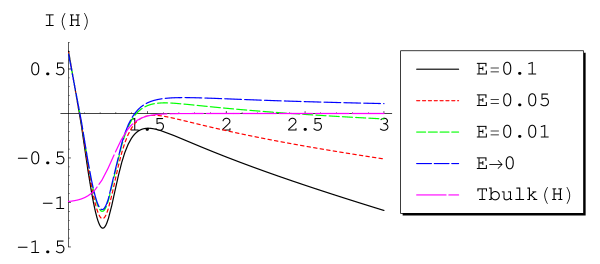
Figure 1: The inflation parameter $I(H)$ as a function of $H$ for $\zeta=8$, $\sigma=1.28$ and for different values of $E$ in $\tau$ units.

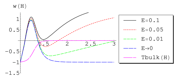
Figure 2: Equation of state parameter $w(H)$ as a function of $H$ for $\zeta=8$, $\sigma=1.28$ and for different values of $E$ in $\tau$ units.

If we switch off the gravitational field on the moving brane then, the mirage effect [20] gives only the late accelerating phase as the probe brane is approaching the bulk. If we switch off the mirage contribution then the brane-universe has the early inflationary phase, where the tachyon field condenses, near the top of the geometrical tachyon potential. If we decouple the bulk tachyon field from the start, having a probe brane moving in the background of other D3-branes then, we have a very short inflationary period in the top of the geometrical tachyon potential. This can be attributed to the presence of the gravitational field on the brane.

4. Conclusions and Discussion

We have studied the movement of a probe D3-brane in the background of a D3-brane solution of Type-0 string theory. We have shown that this movement can be described by the rolling of the geometrical tachyon down its potential. We found that the presence of the bulk tachyon of the Type-0 theory, modifies the potential of the geometrical tachyon. This modification changes the height and the shape of the potential. Solving the classical equations of motion, we analysed the influence of the bulk tachyon to the geometrical tachyon dynamics as it rolls down its potential.

We also studied the cosmological evolution of the brane-universe on the D3-brane as it moves in this background string theory. We introduced a scalar curvature term on the moving brane and we showed that the geometrical tachyon field rolls down its potential under the influence of its own gravitational field and the gravitational field of the background. This results in a cosmological evolution on the moving brane.

We found that there is a choice of parameters, for which early time inflation occurs where the bulk tachyon field condenses at weak coupling. This coincides with the UV fixed point of the RG flows of the bulk Type-0 theory. At this limit, the string coupling is weak and the D3-brane exact solution can be trusted. In the geometrical tachyon picture, this happens near the top of the geometrical tachyon potential. As the geometrical tachyon rolls down its potential, the inflation ends, and as the bulk tachyon asymptotes to zero reaching the IR fixed point of the background theory, the brane-universe enters a late accelerating phase. This happens when the geometrical tachyon reaches the bottom of the potential.

For the same choice of the parameters, the equation of state parameter $w$, starts with the value $w=-1$ in the early inflationary phase, and passing from positive values relaxes again to $w=-1$, in the late accelerating phase. The whole evolution of $w$ occurs without the need of introducing any dark matter or dark energy. It is the dynamics of the bulk theory that drives the whole evolution. Of course for a realistic cosmological evolution of the brane-universe, matter fields have to be introduced on the brane to account for the diversity of matter we observe in our universe.

Type-0 is an interesting string background. We are however, far away from understanding its full dynamics and its connection to the boundary open string theory. Only very limited solutions are known near the conformal fixed points of the theory. If for example more general solutions of the Type-0 string background were known with non-constant tachyon and dilaton fields, the coupling of the bulk tachyon to the geometrical potential would have been a function of the distance $r$ from the bulk Dp-branes. The geometrical tachyon potential then, would get $r$-dependent modifications effecting the dynamics of the geometrical tachyon as it rolls down its potential and its cosmological evolution.

This work provides some evidence that closed tachyon condensation may have some important consequences on the cosmological evolution of the boundary theory. Of course we do not fully understand the dynamics of the closed tachyon condensation and its connection to the gravitational dynamics, but nevertheless we provided an example in which the condensation of the bulk tachyon, except that it stabilizes the bulk theory, it is responsible for the inflation on the boundary theory.

More work is needed to understand the phenomenological aspects of the inflation on the brane, like how long it lasts, what are the scalar perturbations produced during inflation, what is the mechanism for reheating. Can the condensation of the bulk tachyon provide the energy needed for the reheating? However, there is a drawback in these considerations, because the relation (3.5) indicates that the kinetic energy of the geometrical tachyon field is not small and it can not be ignored compared to unity and hence slow-roll inflation can not be applied. This can be understood because of the strong bulk effects of the bulk tachyon condensation.

Our final remark conserns the consistency of our approach. Let us recall what happens in the DGP model [43]. We have a static brane in a time dependent five-dimensional pure gravitational bulk. As it was showed in [45, 46], the introduction of a four-dimensional scalar curvature term on the brane, simply redefines the energy momentum tensor on the brane. If we go to the picture in which the brane is moving and the bulk is static, it can be shown [47, 48], that the $R$ term has the same effect, it redefines the energy momentum tensor in the junctions conditions which play the r$\hat{o}$le of the equations of motion of the moving brane. In both pictures, there is an effective four-dimensional Einstein equation which describes consistently the cosmological evolution on the brane.

In the case of a Dp-brane moving in the background of other Dp-branes the situation is much more difficult [49]. The Dp-branes of the bulk are solutions of a complicated usually string theory and the only information we can get on the brane is only through the DBI action. For this reason we use the rolling tachyon picture which is described by a simple DBI action. In our case, the coupling of gravity on the moving brane complicates further the picture. Our basic assumption is the probe brane approximation. There is no backreaction between the brane and the bulk. As the brane moves in the gravitational field of the background branes it does not disturb this background. This assumption led us to the Friedmann equation (3.17).

5. Acknowlegements

Work supported by (EPEAEK II)-Pythagoras (co-funded by the European Social Fund and National Resources). We thank Malcolm Fairbairn, Ansar Fayyazuddin, Fawad Hassan, Alex Kehagias, George Kofinas, M. Sami, John Ward for very helpful discussions, comments and remarks.

References

- [1] W. Taylor, “Lectures on D-branes, tachyon condensation, and string field theory,” [arXiv:hep-th/0301094].
- [2] A. Sen, “Tachyon dynamics in open string theory,” Int. J. Mod. Phys. A 20, 5513 (2005) [arXiv:hep-th/0410103].
- [3] A. Sen, “Rolling tachyon,” JHEP 0204, 048 (2002) [arXiv:hep-th/0203211].
- [4] A. Sen, “Tachyon matter,” JHEP 0207, 065 (2002) [arXiv:hep-th/0203265].
- [5] M. Gutperle and A. Strominger, “Spacelike branes,” JHEP 0204, 018 (2002) [arXiv:hep-th/0202210].
- [6] A. Maloney, A. Strominger and X. Yin, “S-brane thermodynamics,” JHEP 0310, 048 (2003) [arXiv:hep-th/0302146].
- [7] M. Headrick, S. Minwalla and T. Takayanagi, “Closed string tachyon condensation: An overview,” Class. Quant. Grav. 21, S1539 (2004) [arXiv:hep-th/0405064].
- [8] M. R. Garousi and R. C. Myers, “World-volume interactions on D-branes,” Nucl. Phys. B 542, 73 (1999) [arXiv:hep-th/9809100].
- [9] M. R. Garousi, “String scattering from D-branes in type 0 theories,” Nucl. Phys. B 550, 225 (1999) [arXiv:hep-th/9901085].
- [10] I. R. Klebanov and A. A. Tseytlin, “Asymptotic freedom and infrared behavior in the type 0 string approach to gauge theory,” Nucl. Phys. B 547, 143 (1999) [arXiv:hep-th/9812089].
- [11] A. M. Polyakov, “The wall of the cave,” Int. J. Mod. Phys. A 14, 645 (1999) [arXiv:hep-th/9809057].
- [12] I. R. Klebanov and A. A. Tseytlin, “D-branes and dual gauge theories in type 0 strings,” Nucl. Phys. B 546, 155 (1999) [arXiv:hep-th/9811035].
- [13] I. R. Klebanov, “Tachyon stabilization in the AdS/CFT correspondence,” Phys. Lett. B 466, 166 (1999) [arXiv:hep-th/9906220].
- [14] M. Bianchi and A. Sagnotti, Phys. Lett. B 247, 517 (1990).
- [15] J. A. Minahan, “Glueball mass spectra and other issues for supergravity duals of QCD JHEP 9901, 020 (1999) [arXiv:hep-th/9811156]; J. A. Minahan, “Asymptotic freedom and confinement from type 0 string theory,” JHEP 9904, 007 (1999) [arXiv:hep-th/9902074].
- [16] F. Bigazzi, “RG flows toward IR isolated fixed points: Some type 0 samples,” JHEP 0106, 068 (2001) [arXiv:hep-th/0101232].
- [17] G. T. Horowitz and A. Strominger, “Black strings and P-branes,” Nucl. Phys. B 360, 197 (1991).
- [18] A. Kehagias and E. Kiritsis, “Mirage cosmology,” JHEP 9911, 022 (1999) [arXiv:hep-th/9910174].
- [19] R. Grena, S. Lelli, M. Maggiore and A. Rissone, “Confinement, asymptotic freedom and renormalons in type 0 string duals,” JHEP 0007, 005 (2000) [arXiv:hep-th/0005213].
- [20] E. Papantonopoulos and I. Pappa, “Type 0 brane inflation from mirage cosmology,” Mod. Phys. Lett. A 15, 2145 (2000) [arXiv:hep-th/0001183]; E. Papantonopoulos and I. Pappa, “Cosmological evolution of a brane universe in a type 0 string background,” Phys. Rev. D 63, 103506 (2001) [arXiv:hep-th/0010014].
- [21] C. P. Burgess, N. E. Grandi, F. Quevedo and R. Rabadan, “D-brane chemistry,” JHEP 0401, 067 (2004) [arXiv:hep-th/0310010].
- [22] K. L. Panigrahi, “D-brane dynamics in Dp-brane background,” Phys. Lett. B 601, 64 (2004) [arXiv:hep-th/0407134].
- [23] O. Saremi, L. Kofman and A. W. Peet, “Folding branes,” Phys. Rev. D 71, 126004 (2005) [arXiv:hep-th/0409092].
- [24] D. Kutasov and V. Niarchos, “Tachyon effective actions in open string theory,” Nucl. Phys. B 666, 56 (2003) [arXiv:hep-th/0304045].
- [25] D. Kutasov, “D-brane dynamics near NS5-branes,” [arXiv:hep-th/0405058].
- [26] D. Kutasov, “A geometric interpretation of the open string tachyon,” [arXiv:hep-th/0408073].
- [27] M. Billo, B. Craps and F. Roose, “Ramond-Ramond couplings of non-BPS D-branes,” JHEP 9906, 033 (1999) [arXiv:hep-th/9905157].
- [28] C. Kennedy and A. Wilkins, “Ramond-Ramond couplings on brane-antibrane systems,” Phys. Lett. B 464, 206 (1999) [arXiv:hep-th/9905195].
- [29] A. Sen, “Dirac-Born-Infeld action on the tachyon kink and vortex,” Phys. Rev. D 68, 066008 (2003) [arXiv:hep-th/0303057].
- [30] K. Okuyama, “Wess-Zumino term in tachyon effective action,” JHEP 0305, 005 (2003) [arXiv:hep-th/0304108].
- [31] J. Kluson, “Tachyon kink on non-BPS Dp-brane in the general background,” JHEP 0510, 076 (2005) [arXiv:hep-th/0508239].
- [32] A. Sen, “Field theory of tachyon matter,” Mod. Phys. Lett. A 17, 1797 (2002) [arXiv:hep-th/0204143].
- [33] A. Sen, “Time evolution in open string theory,” JHEP 0210, 003 (2002) [arXiv:hep-th/0207105].
- [34] A. Sen, “Time and tachyon,” Int. J. Mod. Phys. A 18, 4869 (2003) [arXiv:hep-th/0209122].
- [35] J. Kluson, “Non-BPS Dp-brane in Dk-brane background,” JHEP 0503, 044 (2005) [arXiv:hep-th/0501010].
- [36] J. Kluson, “Note about non-BPS and BPS Dp-branes in near horizon region of N Dk-branes,” JHEP 0503, 071 (2005) [arXiv:hep-th/0502079].
- [37] A. Mazumdar, S. Panda and A. Perez-Lorenzana, “Assisted inflation via tachyon condensation,” Nucl. Phys. B 614, 101 (2001) [arXiv:hep-ph/0107058]; M. Fairbairn and M. H. G. Tytgat, “Inflation from a tachyon fluid?,” Phys. Lett. B 546, 1 (2002) [arXiv:hep-th/0204070]; A. Feinstein, “Power-law inflation from the rolling tachyon,” Phys. Rev. D 66, 063511 (2002) [arXiv:hep-th/0204140]; M. Sami, P. Chingangbam and T. Qureshi, “Aspects of tachyonic inflation with exponential potential,” Phys. Rev. D 66, 043530 (2002) [arXiv:hep-th/0205179]; M. Sami, “Implementing power law inflation with rolling tachyon on the brane,” Mod. Phys. Lett. A 18, 691 (2003) [arXiv:hep-th/0205146]; Y. S. Piao, R. G. Cai, X. m. Zhang and Y. Z. Zhang, “Assisted tachyonic inflation,” Phys. Rev. D 66, 121301 (2002) [arXiv:hep-ph/0207143]. A. Ghodsi and A. E. Mosaffa, “D-brane dynamics in RR deformation of NS5-branes background and tachyon cosmology,” Nucl. Phys. B 714, 30 (2005) [arXiv:hep-th/0408015].
- [38] L. Kofman and A. Linde, “Problems with tachyon inflation,” JHEP 0207, 004 (2002) [arXiv:hep-th/0205121].
- [39] G. W. Gibbons, “Cosmological evolution of the rolling tachyon,” Phys. Lett. B 537, 1 (2002) [arXiv:hep-th/0204008]; S. Mukohyama, “Brane cosmology driven by the rolling tachyon,” Phys. Rev. D 66, 024009 (2002) [arXiv:hep-th/0204084]; T. Padmanabhan, “Accelerated expansion of the universe driven by tachyonic matter,” Phys. Rev. D 66, 021301 (2002) [arXiv:hep-th/0204150]; M. C. Bento, O. Bertolami and A. A. Sen, “Tachyonic inflation in the braneworld scenario,” Phys. Rev. D 67, 063511 (2003) [arXiv:hep-th/0208124].
- [40] H. Yavartanoo, “Cosmological solution from D-brane motion in NS5-branes background,” arXiv:hep-th/0407079.
- [41] S. Thomas and J. Ward, “Inflation from geometrical tachyons,” Phys. Rev. D 72, 083519 (2005) [arXiv:hep-th/0504226].
- [42] S. Panda, M. Sami and S. Tsujikawa, “Inflation and dark energy arising from geometrical tachyons,” arXiv:hep-th/0510112; S. Panda, M. Sami, S. Tsujikawa and J. Ward, “Inflation from D3-brane motion in the background of D5-branes,” arXiv:hep-th/0601037; B. Gumjudpai, T. Naskar and J. Ward, “A quintessentially geometric model,” arXiv:hep-ph/0603210.
- [43] G. R. Dvali, G. Gabadadze and M. Porrati, “4D gravity on a brane in 5D Minkowski space,” Phys. Lett. B 485, 208 (2000) [arXiv:hep-th/0005016].
- [44] J. Y. Kim, “Brane inflation in tachyonic and non-tachyonic type 0B string theories,” Phys. Rev. D 63, 045014 (2001) [arXiv:hep-th/0009175]; D. A. Steer and M. F. Parry, “Brane cosmology, varying speed of light and inflation in models with one or Int. J. Theor. Phys. 41, 2255 (2002) [arXiv:hep-th/0201121]; D. Youm, “Brane inflation in the background of D-brane with NS B field,” Phys. Rev. D 63, 125019 (2001) [arXiv:hep-th/0011024]. D. Youm, “Closed universe in mirage cosmology,” Phys. Rev. D 63, 085010 (2001) [Erratum-ibid. D 63, 129902 (2001)] [arXiv:hep-th/0011290]; J. Y. Kim, “Mirage cosmology in M-theory,” Phys. Lett. B 548, 1 (2002) [arXiv:hep-th/0203084]; T. Boehm and D. A. Steer, “Perturbations on a moving D3-brane and mirage cosmology,” Phys. Rev. D 66, 063510 (2002) [arXiv:hep-th/0206147]; P. Bozhilov, “Probe branes dynamics in nonconstant background fields,” arXiv:hep-th/0206253; E. Papantonopoulos and V. Zamarias, “AdS/CFT correspondence and the reheating of the brane-universe,” JHEP 0410, 051 (2004) [arXiv:hep-th/0408227]; P. S. Apostolopoulos, N. Brouzakis, E. N. Saridakis and N. Tetradis, “Mirage effects on the brane,” Phys. Rev. D 72, 044013 (2005) [arXiv:hep-th/0502115]; D. H. Jeong and J. Y. Kim, “Mirage cosmology with an unstable probe D3-brane,” Phys. Rev. D 72, 087503 (2005) [arXiv:hep-th/0502130]; A. Psinas, “Mirage cosmology of U(1) gauge field on unstable D3 brane universe,” [arXiv:hep-th/0509001]; A. Psinas, “Quantum cosmology aspects of D3 branes and tachyon dynamics,” [arXiv:hep-th/0511270].
- [45] G. Kofinas, “General brane cosmology with (4)R term in (A)dS(5) or Minkowski bulk,” JHEP 0108, 034 (2001) [arXiv:hep-th/0108013].
- [46] K. i. Maeda, S. Mizuno and T. Torii, “Effective gravitational equations on brane world with induced gravity,” Phys. Rev. D 68, 024033 (2003) [arXiv:gr-qc/0303039].
- [47] C. Csaki, J. Erlich and C. Grojean, “Gravitational Lorentz violations and adjustment of the cosmological constant in asymmetrically warped spacetimes,” Nucl. Phys. B 604, 312 (2001) [arXiv:hep-th/0012143]; P. Bowcock, C. Charmousis and R. Gregory, “General brane cosmologies and their global spacetime structure,” Class. Quant. Grav. 17, 4745 (2000) [arXiv:hep-th/0007177].
- [48] B. Cuadros-Melgar and E. Papantonopoulos, “The need of dark energy for dynamical compactification of extra dimensions on the brane,” Phys. Rev. D 72, 064008 (2005) [arXiv:hep-th/0502169].
- [49] E. Kiritsis, “D-branes in standard model building, gravity and cosmology,” Fortsch. Phys. 52, 200 (2004) [Phys. Rept. 421, 105 (2005)] [arXiv:hep-th/0310001].