A note on the stability of axionic D-term s-strings

Abstract

We investigate the stability of a new class of BPS cosmic strings in N=1 supergravity with D-terms recently proposed by Blanco-Pillado, Dvali and Redi. These have been conjectured to be the low energy manifestation of D-strings that might form from tachyon condensation after D- anti-D-brane annihilation in type IIB superstring theory. There are three one-parameter families of cylindrically symmetric one-vortex solutions to the BPS equations (tachyonic, axionic and hybrid). We find evidence that the zero mode in the axionic case, or $s-$strings, can be excited. Its evolution leads to the decompactification of four-dimensional spacetime at late times, with a rate that decreases with decreasing brane tension.

Recently Blanco-Pillado, Dvali and Redi have proposed a model to describe a D-brane anti-D-brane unstable system after compactification to four dimensions BDR . In the type IIB case, the tension of the branes appears in the four-dimensional effective theory as a constant Fayet Iliopoulos term which allows for the existence of non-singular BPS axion-dilaton strings generalising earlier work by HN ; BDP ; DBD in heterotic scenarios.

It was shown that this model contains three different families of BPS cosmic string solutions: tachyonic or $\phi$-strings, with winding $n$ (see also DKP ), axionic or $s$-strings with winding $m$ and a third type which is the special case where the following relation is satisfied: $q|m|=|n|$. We are using the same notation of BDR . We call the third type hybrid strings. Each of the families is parametrized by a real number, $\kappa$, defined by the relation:

$$s=2\frac{\delta}{q}(|n|-q|m|)\log r-2\frac{\delta}{q}\log|\phi|+\kappa.$$ (1)

In the first two families the parameter $\kappa$ is associated to a zero mode that connects vortex solutions with different core radius and equal magnetic flux, as can be seen by setting:

$$k=2\frac{\delta}{q}(|n|-q|m|)\log R$$ (2)

In this way $R$ gives the scale of the core radius. In the third case the same parameter measures which of the fields, the dilaton or the tachyon, contributes more to compensate the Fayet-Iliopoulos term.

Supergravity effects were considered in BDR and, as expected on general grounds UAD ; DHKLZ , the zero mode survives the coupling to supergravity.

The $s$-strings are peculiar . The authors of BDR argued that they should be associated with D anti-D bound states that are unstable in ten dimensions, and therefore only exist after compactification. They also noted that they share some features with semilocal strings in the Bogomolnyi limit AV . In the semilocal case any excitation of the zero mode H leads invariably to the spread of the magnetic field and the eventual disappearance of the strings leese .

We have studied numerically the dynamics of this zero mode and we find that also in the $s$-string case it can be excited and will lead to the dissolution of the strings. Since in this process the field $s$ grows without bound, and therefore also the compactification volume modulus, our result would appear to imply the decompactification of spacetime from four to ten dimensions at late times.

We start by briefly reviewing the model of BDR and the three families of BPS strings. We then analyse the zero mode numerically and conclude that it can be excited. For comparison, we show the results of the same analysis on the $\phi$-string, where a perturbation of the string leads to some oscillations but no runaway behaviour.

I The model

The authors of BDR proposed a supersymmetric abelian Higgs model containing a vector superfield $V$ and $N$ chiral superfields. Here we only need to consider one chiral superfield $\Phi$ with charge $q$, that represents the tachyon. The model also involves an axion-dilaton superfield $S$ which is coupled to the gauge multiplet in the usual way. Its lowest component is $s+ia$ where the axion $a$ is the four-dimensional dual of the Ramond-Ramond two-form zero mode after compactification. Its scalar partner $s$ is some combination of the dilaton and the volume modulus. We take the Kähler form to be $K=-M_{p}^{2}\log(S+\bar{S})$ and the gauge kinetic function are set to be constant, $f(S)=1/g^{2}$, where $g$ is the gauge coupling. With this choice, there is no $aF_{\mu\nu}\tilde{F}^{\mu\nu}$ term in the action. The $U(1)$ symmetry is not anomalous, it is the diagonal combination of the $U(1)$s from the D- anti D system.

In component notation the bosonic sector of the lagrangian, after eliminating the auxiliary field from the vector multiplet, is:

$$\mathscr{L} = -|D_{\mu}\phi|^{2}-K_{S\bar{S}}|D_{\mu}S|^{2}-\scriptstyle\frac{1}{4}\displaystyle g^{-2}F^{\mu\nu}F_{\mu\nu}{}$$ (3)

$${}-\scriptstyle\frac{1}{2}\displaystyle g^{2}(\xi+2\delta K_{S}-q|\phi|^{2})^{2}.$$

$K_{S}$ and $K_{S\bar{S}}$ represent the derivatives of the Kahler potential respect to the fields $S$ and $\bar{S}$. $\phi$ is the lowest component of the chiral field field, $A_{\mu}$ is the $U(1)$ gauge field, and $F_{\mu\nu}=\partial_{\mu}A_{\nu}-\partial_{\nu}A_{\mu}$ the associated abelian field strength,

$$D_{\mu}\phi=\partial_{\mu}\phi-iqA_{\mu}\phi,\qquad D_{\mu}S=\partial_{\mu}S+i2\delta A_{\mu}.$$ (4)

$\delta$ is the coupling of the axion to the gauge field. In the case of anomalous $U(1)$, where f(S) = S, it is called the Green-Schwarz parameter and is fixed by the value of the anomaly. Here $\delta$ is not determined.

It is convenient to write the bosonic part of the lagrangian using the rescalings:

$$\phi=\sqrt{\xi/q}\;\hat{\phi} s=\delta M_{p}^{2}/\xi\;\hat{s} a=2\delta/q\;\hat{a}$$

$$A_{\mu}=g\sqrt{\xi/q}\;\hat{A}_{\mu} x=(g\sqrt{\xi q})^{-1}\;\hat{x}\ ,$$ (5)

With these definitions the axion $\hat{a}$ is defined modulo $2\pi$, and $\delta$ is rescaled away. After dropping the hats, the bosonic sector of the lagrangian reads:

$$\mathscr{L}(\xi g)^{-2} = -|D_{\mu}\phi|^{2}-\scriptstyle\frac{1}{4}\displaystyle(\alpha s)^{-2}(\partial_{\mu}s)^{2}-(\alpha/s)^{2}(\partial_{\mu}a+A_{\mu})^{2}{}$$ (6)

$${}-\scriptstyle\frac{1}{4}\displaystyle F^{\mu\nu}F_{\mu\nu}-\scriptstyle\frac{1}{2}\displaystyle(1-s^{-1}-|\phi|^{2})^{2}\ ,$$

with $D_{\mu}\phi=\partial_{\mu}\phi-iA_{\mu}\phi$, and $\alpha^{2}=\xi/(qM_{p}^{2})$. Note that, since $\alpha$ is the symmetry breaking scale in Plank units, ignoring supergravity and superstring corrections would only be a consistent approximation for $\alpha\ll 1$. However, this limit is difficult to analyze numerically. We will present numerical results for $\alpha=1$ and argue separately on the effect of lowering $\alpha$.

To study straight vortices along, say, the $z-$direction, we drop the z dependence and set $A_{z}=0$. For time independent configurations and defining $\tilde{S}=s+2i\alpha^{2}a$, and $\tilde{D}_{\mu}\tilde{S}=\partial_{\mu}\tilde{S}+2i\alpha^{2}A_{\mu}$, the energy functional can be written in the Bogomolnyi form:

$$\mathscr{E}(\xi g)^{-2} = |(D_{x}\pm iD_{y})\phi|^{2}+\scriptstyle\frac{1}{4}\displaystyle(\alpha s)^{-2}|(\tilde{D}_{x}\pm i\tilde{D}_{y})\tilde{S}|^{2}{}$$ (7)

$${}+\scriptstyle\frac{1}{2}\displaystyle(F_{xy}\mp(1-s^{-1}-|\phi|^{2}))^{2}\pm F_{xy}{}$$

$${}\mp i[\partial_{x}(\phi^{*}D_{y}\phi)-\partial_{y}(\phi^{*}D_{x}\phi)]{}$$

$${}\pm i\scriptstyle\frac{1}{2}\displaystyle\alpha^{-2}[\partial_{x}(s^{-1}\tilde{D}_{y}\tilde{S})-\partial_{y}(s^{-1}\tilde{D}_{x}\tilde{S})].$$

leading to a bound on the energy per unit length

$$E=\scriptstyle\int\displaystyle d^{2}x\mathscr{E}\geq(\xi g)^{2}\scriptstyle\int\displaystyle d^{2}xF_{xy}.$$ (8)

The bound is attained by the solutions of the Bogomolnyi equations

$$(D_{x}\pm iD_{y})\phi =0$$

$$(\tilde{D}_{x}\pm i\tilde{D}_{y})\tilde{S} =0$$

$$F_{xy}\mp(1-s^{-1}-|\phi|^{2}) =0$$ (9)

We will focus on cylindrically symmetric vortices, that can be described by the following ansatz:

$$\phi=f(r)e^{in\theta} \qquad s^{-1}=h^{2}$$

$$a=m\theta\qquad \qquad A_{\theta}=v(r)/r\ .$$ (10)

(The ansatz for the dilaton makes comparison to the semilocal case easier. Also we shall see that $h$ vanishes in various cases, and with this choice we avoid having to deal with infinities).

With this ansatz the energy density becomes:

$$\mathscr{E}=A(r)^{2}+B(r)^{2}/(\alpha\,h)^{2}+\scriptstyle\frac{1}{2}\displaystyle C(r)^{2}+D(r)^{\prime}/r$$ (11)

and the Bogomolnyi equations

$$A(r) \equiv f^{\prime}-f(|n|-v)/r=0$$

$$B(r) \equiv h^{\prime}-\alpha^{2}h^{3}(|m|-v)/r=0$$ (12)

$$C(r) \equiv v^{\prime}/r-(1-f^{2}-h^{2})=0$$

$$D(r) \equiv v-f^{2}(v-|n|)-h^{2}(v-|m|)=0$$ (13)

The total energy is:

$$E=2\pi\scriptstyle\int\displaystyle drr\mathscr{E}(r)\geq 2\pi v_{\infty}$$ (14)

where $v_{\infty}$ is the asymptotic value of the gauge field profile function for large values of $r$.

The condition $A(r)=B(r)=0$ implies the following relation between the tachyon and the dilaton:

$$1/(\alpha\,h)^{2}=2(|n|-|m|)\log r-2\log f+\kappa.$$ (15)

Depending on the asymptotic value of the profile functions for large values of $r$, $f_{\infty}$, $h_{\infty}$ and $v_{\infty}$, we can classify the solutions to the Bogomolnyi equations in three different families. Each of them is parametrized by the integration constant $\kappa$.

$\bullet$ In the first case,

$$f_{\infty}=1,\quad h_{\infty}=0,\quad v_{\infty}=n\ ,$$ (16)

the tachyon acquires a non vanishing vacuum expectation value far from the center of the string. The magnetic flux of these vortices is induced by the winding of the tachyon, $n$.

The profile function $h(r)$ tends very slowly, (logarithmically), to zero at large $r$. The details about the asymptotics of the fields can be found in BDR . Following Blanco-Pillado et al. we call these vortices $\phi$-strings.

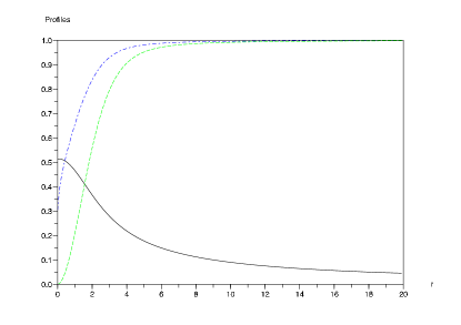
Figure 1: The axion string profile functions, for m=1, n=0, $a(r)$, (upper dashed line), $h(r)$, (middle dashed line) and $f(r)$, (lower solid line), with the size of the condensate, $f_{0}=0.51$.

$\bullet$ In the second case, Fig.(1), the dilaton alone is responsible for compensating the D-term. The function $h(r)$, approaches a non vanishing constant far from the centre of the string, while the tachyon expectation value tends to zero. In this family the magnetic flux is induced by the winding of the axion, $m$.

$$f_{\infty}=0\quad h_{\infty}=1\quad v_{\infty}=m$$ (17)

These vortices have been denominated $s$-strings. They are regular thanks to the constant Fayet-Iliopoulos term

In the previous two families the constant $\kappa$ has the same interpretation. Each value of this parameter is associated to a particular width of the strings.

$\bullet$ For strings of the third family both the tachyon and the dilaton contribute to compensate the $D$-term. This happens when the axion and dilaton have the same winding.

$$f_{\infty}^{2}+h_{\infty}^{2}=1\qquad v_{\infty}=n=m$$ (18)

In this case $f_{\infty}$ and $h_{\infty}$ can have any value as long as the previous relation is satisfied (18). Each particular $f_{\infty}$ can be associated to a single $\kappa$, which means that the interpretation of this parameter is different to the previous two cases, and cannot be related any more to the width of the strings, so we will not discuss it any further.

As can be seen in (13) the derivatives of $h$ scale as $\alpha^{2}$. In the case of the $\phi$-strings, varying $\alpha$ for a fixed value of the integration constant k does not change much the width of the string, but the condensate flattens. In the limit when $\alpha$ is very small the $\phi-$strings are similar to a Nielsen-Olesen string. In the case of $s-$strings the width of the string increases with decreasing $\alpha$, while the condensate does not vary much. In fact, the main effect of decreasing $\alpha$ will be a slowing down of the dynamics.

II Discretized Equations of Motion

The functions $f(r)$, $h(r)$ and $v(r)$ are substituted by the set of quantities $f_{k}$, $h_{k}$ and $v_{k}$ which are the profile functions evaluated in the lattice points $r_{k}=(k+\scriptstyle\frac{1}{2}\displaystyle)\Delta$, where $\Delta$ is the lattice spacing.

We want to analyze the response of the solutions of the Bogomolnyi equations under perturbations. We must make sure that the configurations that we are going to perturb are stationary solutions of the equations of motion. This is automatic in the continuous case but not in an arbitrary discretization.

Following Leese leese we construct a discrete version of the energy functional for static configurations given by:

$$\mathscr{E}_{k}\Delta^{2} = A_{k}^{2}+\frac{4B_{k}^{2}}{\alpha^{2}(h_{k+1}+h_{k})^{2}}+\frac{C_{k}^{2}}{2\Delta^{2}}+\frac{(D_{k+1}-D_{k})}{k+\scriptstyle\frac{1}{2}}\$$ (19)

where

$$A_{k} = f_{k+1}-f_{k}-(n-v_{k})\frac{f_{k+1}+f_{k}}{2k+1},$$

$$B_{k} = h_{k+1}-h_{k}-\alpha^{2}(m-v_{k})\frac{(h_{k+1}+h_{k})^{3}}{2k+1},$$

$$C_{k} = \frac{v_{k+1}-v_{k}}{k+\scriptstyle\frac{1}{2}}-\Delta^{2}(1-h_{k+1}^{2}-f_{k+1}^{2}),$$

$$D_{k} = v_{k}-f_{k}^{2}(v_{k}-n)-h_{k}^{2}(v_{k}-m).$$ (20)

The profile functions are obtained minimizing the total energy for static configurations:

$$E=2\pi\sum_{k=0}^{\infty}\Delta^{2}(k+\scriptstyle\frac{1}{2})\displaystyle\mathscr{E}_{k},$$ (21)

for which the discretized Bogomolnyi equations have to be satisfied: $A_{k}=B_{k}=C_{k}=0$.

The boundary conditions used to solve them are set at the points $r_{0}$ and $r_{1}$. At $r_{0}$ we impose $v_{0}=0$, and at $r_{1}$ we fix the values of $f_{1}$ and $h_{1}$. One of these two has to be tuned in order to obtain the correct asymptotic behavior, and each value of the other one corresponds to a different solution within a family.

The following discretized version of the action is naturally associated to the energy functional (21):

$$S = -2\pi\tau\Delta^{2}\sum_{l,k=0}^{\infty}(k+\scriptstyle\frac{1}{2}\displaystyle)(\mathscr{E}_{k}^{l}-\mathscr{T}_{k}^{l})$$

$$\tau^{2}\mathscr{T}_{k}^{l} = (f_{k}^{l+1}-f_{k}^{l})^{2}+\frac{(h_{k}^{l+1}-h_{k}^{l})^{2}}{\alpha^{2}h_{k}^{2}}-\frac{(a_{k}^{l+1}-a_{k}^{l})^{2}}{(2k+1)\Delta^{4}}\$$ (22)

The superscript $l$ labels the time slices, which are separated by an interval $\tau$.
Here $\mathscr{T}_{k}^{l}$ represents the density of energy associated to the time derivatives.

The equations of motion can be derived from (22) by setting to zero the partial derivatives of the action with respect to the variables $f_{k}^{l}$, $h_{k}^{l}$, $v_{k}^{l}$.

As the solutions of the Bogomolnyi equations are static and minimize the discretized energy functional they must be stationary solutions of the discretized time dependent equations of motion.

The boundary conditions have been implemented using the same method of leese . All the quantities measured take information from a region of radius $r_{cal}=4.5$. The simulation is stopped at $t_{max}=2(r_{max}-r_{cal})$. In this way the region from which we take data is not affected by the presence of the boundary. A typical value for the size of the lattice is $r_{max}=21.5$, but it varies depending on the profile.

During the simulation we keep track of the following quantities:

$$E(l,k_{cal}) = 2\pi\sum_{k=0}^{k_{cal}}\Delta^{2}(k+\scriptstyle\frac{1}{2})\displaystyle\mathscr{E}_{k}^{l}$$ (23)

$$T(l,k_{cal}) = 2\pi\Delta^{2}\sum_{k=0}^{k_{cal}}(k+\scriptstyle\frac{1}{2}\displaystyle)\mathscr{T}_{k}^{l}$$ (24)

$$E_{T}(l,k_{cal}) = \frac{E(l,k_{cal})+T(l,k_{cal})}{E(0,k_{cal})+T(0,k_{cal})}$$ (25)

$$W = 2\pi\Delta^{3}\frac{\sum_{k=0}^{k_{cal}}(k+\scriptstyle\frac{1}{2}\displaystyle)^{2}\mathscr{E}_{k}^{l}}{E(l,k_{cal})}$$ (26)

$$F(l,k_{cal}) = 2\pi(D_{k_{cal}}^{l}-D_{0}^{l})$$ (27)

Here $k_{cal}$ is defined by $r_{cal}=(\scriptstyle\frac{1}{2}\displaystyle+k_{cal})\Delta$.
$E$ is the static energy contained in $r<r_{cal}$, and $T$ the energy due to the time derivatives in the same region. $E_{T}$ is the total energy normalized to the initial value. $W$ is a measure of the width of the string. In (26) the expression in the numerator is similar to the energy functional, but the extra factor $(k+\scriptstyle\frac{1}{2}\displaystyle)$ gives more weight to the energy far away from the core. Then, $W$ increases as the energy spreads. $F$ gives the magnetic flux confined in the region $r<r_{cal}$.

To implement the perturbation, we set a solution of the discrete Bogomolnyi equations in the first time slice $l=0$, and in the second, $l=1$, we put the same solution slightly deformed. We characterize the strength of the perturbation by the fractional change of width between the first, ($l=0$), and second, ($l=1$), time slices:

$$\dot{W}_{0}\equiv(W(l=1)-W(l=0))/W(l=0).$$ (28)

During the simulation we have set $\Delta=0.1$ and $\tau=0.05$, with $\tau/\Delta$ smaller than the Courant number $1/\sqrt{2}$.

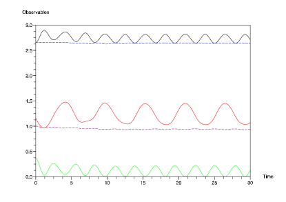
Figure 2: Response of a $\phi-string$ ($n=1,\ m=0$), with $\alpha=1$ and condensate size $h_{1}=0.5$, to a perturbation with strength $\dot{W}_{0}=-0.261$. The plotted lines are, from top to bottom, $E$, $F$, $W$, $E_{T}$ and $T$ (except for $W$ and $E_{T}$, the rest of the plots have been rescaled by a factor of $1/2$ to fit in the window). The core width, $W$, oscillates but is constant on average showing that the zero mode is not excited.

II.1 Tachyonic Strings

In this case to implement the perturbation we take the second time slice to be :

$$f_{k}^{1}=(1+p(r))f_{k}^{0},\quad a_{k}^{1}=(1+p(r))a_{k}^{0}$$

$$h_{k}^{1}=(\;1/(h_{k}^{0})^{2}+2\log(\,1-p(r)\,)\;)^{-1/2}$$ (29)

with the perturbation $p(r)=p_{0}[1-3(r/r_{0})^{2}+2(r/r_{0})^{3}]$ for $r<r_{0}$ and zero otherwise.
The perturbation has been chosen in order to maximize the fraction of energy absorbed by the zero mode. Notice the relation between the perturbations of the tachyon field and the dilaton, and the equation (15) that gives $h$ in terms of $f$, in fact for small values of the parameter $p_{0}$ the perturbed profile approximately satisfies the Bogomolnyi equations. This perturbation gives a coordinate dependence to the integration constant $\kappa$.
The results shown are for a value of $p_{0}$ such that the perturbation initially reduced the width of the string, but the same results are obtained in the opposite case. The parameter $r_{0}$ varies for different initial conditions. In general it has a value close to $r_{0}=2$.

Fig.(2) shows the evolution of a $\phi$-string, with $n=1$, $m=0$ and a core size $h_{1}=0.51$. We show the case $\alpha=1$, which is also the choice made in BDR . The perturbation applied has a strength $\dot{W}_{0}=-0.261$, which corresponds to a $0.4\%$ perturbation in the energy. We have plotted the observables defined in the last section as a function of time. Upper solid line represents $E$, the dashed line just below is the magnetic flux in $r<r_{cal}$, which remains almost constant. The kinetic energy, $T$, is represented by the bottom solid line. The dashed line at the center of the figure is the total energy. Although it can not be clearly seen in the plot, the data tell us that during the period before $t=12$, a fraction of the energy is lost. This is the initial burst of radiation emitted after the perturbation. After that the system reaches a stationary state where all quantities oscillate except the magnetic flux and the total energy.

The remaining solid line in the center is the string width. As the energy contained in the region $r\leq r_{cal}$ remains constant and the width of the vortex oscillates only around the initial value we conclude that this kind of string is stable under this perturbation. The experiment has been repeated in a wide range of the parameters, $p_{0}$, $r_{0}$, and for different initial widths (parametrized by $h_{1}$), and windings, but the results are similar to the ones presented here. Nielsen-Olesen vortices react in the same way to a perturbation, as was shown in leese .

We have repeated the evolution for different values of $\alpha$ but no qualitative change has been observed. As was mentioned before, the smaller the value of $\alpha$, the more similar the $\phi-$string is to a regular Nielsen-Olesen string, which is known to be stable.

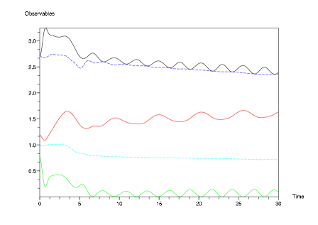
Figure 3: Response of an $s-$string ($n=0$, $m=1$), with $\alpha=1$ and condensate size $f_{1}=0.49$, to a perturbation with strength $\dot{W}_{0}=-0.095$. The plotted lines are, from top to bottom, $E$, $F$, $W$, $E_{T}$ and $T$ (except for $W$ and $E_{T}$, the rest of the plots have been rescaled by a factor of $1/2$ to fit in the window). The core width, $W$, after a transient, oscillates and increases at a constant rate, the zero mode is excited in this case.

II.2 Axionic Strings

The relevant perturbation that excites the zero mode in this case is:

$$f_{k}^{1}=(1-p(r))f_{k}^{0},\quad a_{k}^{1}=(1-p(r))a_{k}^{0}$$

$$h_{k}^{1}=(\;1/(h_{k}^{0})^{2}+2\log(\,1+p(r)\,)\;)^{-1/2}$$ (30)

The result of applying this perturbation with a strength of $\dot{W}_{0}=-0.095$ to an $s$-string, with $\alpha=1$, can be seen in Fig.(3). In this case the perturbation in energy is $2.4\%$. The string has windings $n=0$ and $m=1$, and core size $f_{1}=0.51$. The functions plotted are the same ones that appear in Fig.(2). One of the most relevant features of these plots is that the magnetic flux and the total energy are decreasing with time, which implies that the energy is flowing out from the region $r\leq r_{cal}$, and the magnetic flux is spreading. At the same time the width of the string, ignoring the oscillatory behavior, increases at a constant rate. Before $t=5$ oscillations are noisy. In this period the shock wave produced by the perturbation is still inside $r\leq r_{cal}$.

Although the perturbation was chosen to reduce the core width, the time interval when the core is contracting cannot be seen clearly in the figures. The reason is that the contracting regime ends before the initial burst of radiation comes out from the observed region. As the system is not in a steady state yet, the data are difficult to interpret. We have chosen to show this case because the expanding regime is shown more clearly.

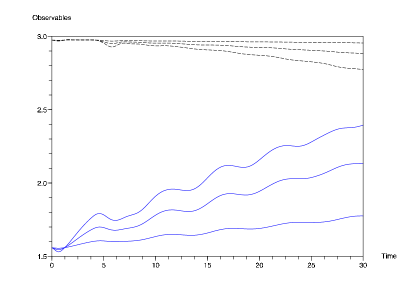
Figure 4: Response of an $n=0$, $m=2$, $\alpha=1$ $s$-string with a core condensate of size $f_{1}=0.51$ to perturbations with different strengths. Dashed lines correspond to $F$, the strength is lowest for the top one. Solid lines represent $W$, the strength is highest for the top one. The strengths are: $\dot{W}_{0}=-0.004$, $-0.014$ and $-0.024$. $F$ is rescaled by a factor of $1/4$. The figure shows how the growth rate of the core increases with the perturbation strength.

Fig.(4) shows the effect of applying perturbations of different strengths to a $n=0$, $m=2$ vortex. In this case the vortex has also a condensate size of $f_{1}=0.51$. The strengths applied are: $\dot{W}_{0}=-0.004$, $\dot{W}_{0}=-0.014$ and $\dot{W}_{0}=-0.024$.

Notice that the bigger the strength of the perturbation, the larger the fraction of magnetic flux lost through the boundary $r=r_{cal}$. The rate of growth of the radius also increases with the strength of the perturbation.

In Fig.(5) it can be seen how the rate of expansion of an $s-$string, ($m=1$, $n=0$), is affected by varying the value of $\alpha$. In this case the perturbation has been chosen to initially increase the core size $\dot{W}_{0}=0.233>0$. As we decrease $\alpha$, keeping the perturbation strength fixed, the rate of expansion of the string decreases. This can be understood from equation (22). The energy associated to the field $h$ scales as the inverse of $\alpha^{2}$. Deviations from the solution to the Bogomolnyi equations cost more energy for smaller values of $\alpha$, thus for a fixed perturbation strength the evolution rates should decrease with $\alpha$. The values of alpha are: $\alpha=0.95$, $0.94$, $0.90$.

The precision of the technique used here does not allow to obtain reliable data for values of $\alpha$ lower than $0.7$, where already the evolution is so slow that it can hardly be appreciated during the time of the simulation. However, note that in these simulations time is measured in units of the inverse of the Higgs mass, thus even for lower values of $\alpha$ decompactification is still possible on cosmological time scales.

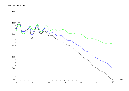
Figure 5: Response of an $n=0$, $m=1$ $s$-string with a core condensate of size $f_{1}=0.51$ to a perturbation with $\dot{W}_{0}=0.233$. The curves represent $F$, the magnetic flux rescaled by a factor of $1/4$. From bottom to top the values of $\alpha$ are are: $\alpha=0.95$, $0.94$ and $0.90$. The figure illustrates the slowing down of the core expansion with decreasing $\alpha$

We are grateful to Jose Blanco-Pillado, Stephen Davis, Koen Kuijken and Jon Urrestilla for very useful discussions. This work is supported by Basque Government grant BF104.203, by the Spanish Ministry of Education under project FPA 2005-04823 and by the Netherlands Organization for Scientific Research (N.W.O.) under the VICI programme. We are also grateful to the ESF COSLAB Programme for incidental support in the initial stages of this work.

References

- (1) J.J. Blanco-Pillado, G. Dvali and M.Redi, Phys.Rev. D72 (2005) 105002 [arXiv: hep-th/0505172]
- (2) J.A. Harvey, S.G. Naculich, Phys. Lett. B217 (1989) 231
- (3) P. Binetruy, C. Deffayet, P. Peter, Phys. Lett. B441 (1998) 52 [arXiv: hep-ph/9807233]
- (4) S.C. Davis, P. Binetruy, A.-C. Davis, Phys. Lett. B611 (2005) 39 [arXiv: hep-th/0501200]
- (5) G. Dvali, R. Kallosh, A. Van Proeyen, JHEP 0401 (2004) 035 [arXiv: hep-th/0312005]
- (6) J. Urrestilla, A. Achúcarro, A.C. Davis, Phys. Rev. Lett. 92 (2004) 251302 [arXiv: hep-th/0402032]
- (7) K. Dasgupta, J.P. Hsu, R. Kallosh, A. Linde, M. Zagermann, JHEP 0408 (2004) 030 [arXiv: hep-th/0405247]
- (8) A. Achúcarro and T. Vachaspati, Phys. Rept. 327 (2000) 347 [arXiv: hep-ph/9904229]
- (9) M. Hindmarsh Phys. Rev. Lett. 68 (1992) 1263
- (10) R.A. Leese, Phys. Rev. D46 (1992) 4677