A Tutorial on Links between Cosmic String Theory and Superstring Theory

Cosmic superstrings are introduced to non-experts. First D-branes and $(p,q)$ strings are discussed. Then we explain how tachyon condensation in the early universe may have produced F, D and $(p,q)$ strings. Warped geometries which can render horizon sized superstrings relatively light are discussed. Various warped geometries including the deformed conifold in the Klebanov-Strassler geometry are reviewed and their warp factors are calculated. The decay rates for strings in the KS geometry are calculated and reasons for the necessity of orientifolds are reviewed. We then outline calculations of the intercommuting probability of F, D and $(p,q)$ strings and explain in detail why cosmic superstring intercommuting probabilities can be small. We explore cosmic superstring networks. Their scaling properties are examined using the Velocity One Scale model and its extra dimensional extensions. Two different approaches and two sets of simulations are reviewed. Finally, we review in detail the gravitational wave amplitude calculations for strings with intercommuting probability $P<1$.

1 Introduction

Cosmic strings and superstrings have been studied for more than 20 years. There has been some cross fertilization of ideas. For example, cosmic string theorists have constructed supersymmetric cosmic superstrings which might model superstrings at low energy [1, 2, 3, 4, 5], and string theorists often use the field theory langauge of effective theories and topological defects to describe superstrings, D-strings and D-branes [6, 7]. However in general, interactions between the cosmic string and superstring communities have been infrequent.

The reasons for this may be as follows. (1) Superstrings have Planckian tensions and observational data precludes such incredibly heavy strings. (2) Twenty years ago Witten showed that long fundamental BPS strings in the most phenomenologically acceptable version of string theory at the time (the heterotic theory) are unstable and hence would never be seen in the sky. Four-dimensional BPS strings are axionic and assuming an axion potential is generated (string theory abhors global continuous symmetries) they bound domain walls which collapse very long string loops. This killed off interest in astrophysical superstrings particularly because it was widely believed that non-BPS strings are also unstable and could not grow to cosmic sizes. (3) Despite being speculative, cosmic string theory is constrained by the latest observational data. Since the observed world is four dimensional and for example, the extra moduli fields originating from say stringy compactifications of the extra dimensions are not seen, the cosmic string community has understandably avoided superstrings. (4) Until recently, string theorists have by and large avoided cosmological issues - the favorite subject of many cosmic string theorists.

The climate has now changed. Cosmic string theorists are now more open to extra dimensions and the extra machinery of string theory [8, 9]. Also, string theorists are much more interested in cosmology and possible string theory imprints in the sky [10].

In fact the picture that is now emerging is that long superstrings may be stable and may appear at the same energy as GUT scale cosmic strings. These strings are similar to cosmic strings in that they radiate, generate networks, lense distant objects, etc. From the point of view of cosmic string theorists, this is interesting, since much of the machinery and work from 15 years ago carries over to these new stringy objects, albeit with some crucial differences. From the string theory point of view, this is very exciting because by positing stable cosmic superstrings which radiate in an experimentally accessible band, they have stumbled upon a possible string theory object which may be detected in our lifetime. The most general cosmic superstrings are $(p,q)$ strings which package fundamental and solitonic strings into a single object [11, 12, 13].

The technical developments which have led to this emerging picture are the following. (1) The AdS-CFT correspondence has taught theorists that gauge strings and superstrings are two faces of the same object [14, 15, 16]. Thus the strings that cosmic string theorists and superstring theorists have been studying may be the same objects. (2) The discovery of D-branes as anchors for open string endpoints and as possible hyperplanes where we may live has made Type II and Type I string theories phenomenologically much more attractive and has opened up many new avenues for string model building, moduli fixing and string cosmology [17, 18, 19, 20, 21, 22]. In these theories it is possible to construct long macroscopic strings which are not BPS but are nonetheless stable and potentially observable [23]. (3) The study of more general extra dimensional compactifications has led to the investigation of warped compactifications in which superstring tensions can be reduced by an enormous factor of $\sim 10^{-8}$ [22]. Superstrings in such warped geometries will not overclose the universe and are potentially cosmologically viable. Furthermore, the warping can turn previously unstable non-BPS strings into “stable” non-BPS strings. (4) The realization that gravitational waves from strings with cusps is very non-Gaussian means that gravitational waves from superstrings in a warped geometry may be observable by gravitational wave experiments like LIGO and LISA [24, 25, 26].

Let us trace the recent history of cosmic superstrings to understand which of their properties are model dependent and which are generic.

Type II or Type I cosmic superstrings recently appeared in brane inflation models [27, 28, 29, 30, 31]. These models, tried to use the flexibility of objects (branes) moving in extra dimensions to produce inflation. Inflation in these scenarios ended in a phase transition mediated by so-called open string tachyons [32]. This violent phase transition left in its wake daughter objects, as many field theoretic phase transitions do, which are solitonic “D-strings” and long fundamental “F-strings” [27, 28]. This led to excitement that string-theoretic brane inflation produces cosmic strings. However, there were significant problems with these brane inflation models. The tensions of the strings they produced were not necessarily small and had to be finetuned [30, 31]. Eventually the brane inflation picture was refined by models in which the extra dimensions of the models are “dynamically” fixed by using a more general warped metric which depends on extra dimensional coordinates [33, 34, 35, 36]. The warping naturally leads to low tension non-BPS cosmic strings which are stable. The same trick of warping the large four dimensions was used by Randall and Sundrum and these flux compactification models are string theoretic realizations of the Randall Sundrum model [37, 38].

It might thus seem that cosmic superstrings are relevant only if brane inflation occurred and if our world is warped by extra dimensions. However, we will take a more general point of view. If a tachyonic (non-supersymmetric) phase transition ever happened in an expanding universe (after inflation) and if our 4D metric contains traces of the extra dimensions via some sort of warping- then cosmic superstrings will inevitably appear. And while brane inflation, though interesting may be farfetched, in the author’s point of view it would not be surprising if some non-supersymmetric phase transition like tachyon condensation on a space filling object occurred and if our 4D metric contains traces of the extra dimensions. Given those two ingredients, cosmic superstrings are reasonably plausible and the brane inflation picture is not crucial for their relevance.

In fact the problem might not be how string theory can be coaxed to produce cosmic strings, but that it produces too many and too many kinds of cosmic superstrings. A cosmic superstring may be a $Dp$ brane wrapped on a $(p-1)$ dimensional compact cycle. Common (Calabi-Yau) compactifications often have thousands of 3D $S^{3}$ and 2D $S^{2}$ cycles and a string obtained by wrapping on one $S^{3}$ is different from a string obtained by wrapped on a different $S^{3}$. Hence, there are thousands of kinds of cosmic strings in string theory. Also, dimensional reduction of ten dimensional string fields to four dimensions gives something like 70 scalar fields. In 4D, a string can magnetically couple to a scalar and hence 70 types of string can appear just from the existence of the extra dimensions [39].

This review is a writeup from various lectures delivered at various places from 2004-2005, for example at the Cosmology in Laboratory Conference in Ambleside, UK in 2004, Imperial College, Dhaka University and the University of Leiden. Many of the most contemporary remarks in the review originate from talks, discussions and debates at a Cosmic Superstrings Workshop at the Institut Henri Poincare in Paris from September 22-27, 2005.

The review is aimed at students. Hence, it is detailed and works out some of the more important calculations in the subject. Also because cosmic superstrings involve a wide array of tools, from boundary conformal field theory to calculations of the dependence of a gravitational wave’s amplitude on the burst frequency – it is felt that others may also benefit from the detail. In particular, the two specialist topics of string scattering and astrophysical traces of cosmic strings are reviewed in detail.

The review is structured as follows. First we try to introduce D-branes to the novice and explain why the appearance of extended objects like D-branes may be natural in higher dimensional theories. Then we show how D-strings are topological defects of an effective supergravity theory and discuss how string duality leads to the more general $(p,q)$ strings. We examine some properties of $(p,q)$ strings like the junction conditions. We then explain one way to think about galaxy sized superstrings and discuss their links to the more familiar cosmic strings. In the next section we discuss how tachyon condensation in the early universe can produce objects like $D3$ braneworlds and D-strings via the Kibble mechanism. We try to explain why tachyon condensation may be natural in the early universe and how it can be thought of as another symmetry restoring transition at high temperature. We then explain how long fundamental strings are produced as remnants of tachyon condensation. The standard boundary conformal field theory calculation of the number density of produced strings is briefly outlined. We then ask how can one make such strings reasonable – how can one suppress their tension? Various warped geometries which lower the tension are discussed and the popular Klebanov-Strassler deformed conifold is reviewed and its warp factor is calculated. An element of such models confusing to cosmologists is orientifolding. Reasons why orientifolds must appear are discussed. A by-product of the orientifolding is that F and D strings are not BPS in these models and hence are not axionic. We calculate the annihilation rates and show that they are exponentially small. We also show why Type II fundamental strings are axionic and how membrane instantons lead to an axion potential. Next, we investigate, F, D and $(p,q)$ string scattering and calculate their scattering amplitudes and the probability that reconnection will occur. We review D-D scattering in some detail and discuss the effect of compactification if the strings are free to move in the extra dimensions or are confined by some potential to particular points. We explain how quantum fluctuations blur the positions of strings classically fixed in space by a potential.

In the last third of the review we discuss observational issues. Scaling for cosmic string networks is reviewed. We review a simulation of a (3+1) dimensional $(p,q)$ string network and ask what happens when strings can move in the extra dimensions. This motivates our review of the generalized extra dimensional velocity one scale model and its insights on the effects of extra dimensions and an intercommuting probability $P<1$. In the final section, we investigate gravitational wave signatures from cosmic superstrings. First basic properties of cusps on cosmic strings are reviewed and then the gravitational burst amplitude $h$ is calculated and its dependence on the intercommuting probability $P$.

A note on the literature: Other reviews of cosmic superstrings are [8, 9, 10]. The central papers on which this review is based are [23, 22, 24, 25, 26, 28, 40, 41, 42, 43].

2 What are D-branes? What is their relation to cosmic strings?

2.1 Extra dimensions naturally give extra extended objects

The variety of antisymmetric fields a theory can possess increases with the spacetime dimension. Because gauge field strengths are antisymmetric, the number of possible field strengths also increases with dimension. Since field strengths give rise to gauge fields which couple to objects carrying some sort of charge, as the variety of field strengths increases with dimension so does the variety of charge carrying objects. Such objects are known as branes. In general a theory living in $d$ spacetime dimensions can have field strengths with at most $d/2$ indices and gauge fields with at most $d/2-1$ indices [44]. The upper bound appears because field strengths with more than $d/2$ indices can be related to new field strengths with less than $d/2$ indices by epsilon contraction. For example, in (3+1)D a 3-form field strength $F_{\mu\nu\lambda}$ can be related to a 1-form field $\tilde{F}_{\rho}$ by contraction with the (3+1)D epsilon tensor $\tilde{F}_{\rho}={\epsilon^{\mu\nu\lambda}}_{\rho}F_{\mu\nu\lambda}$ – this is called Hodge duality. The gauge field, $A_{\mu\nu}$ corresponding to $F_{\mu\nu\lambda}$ is then mapped to a scalar gauge field $A$ such that $\partial_{\rho}A=F_{\rho}$.

String theory which lives in ten dimensions by the same reasoning can have field strengths with up to $\frac{10}{2}=5$ indices. Field strengths with say 6 indices, such as $F_{\mu_{1}\cdots\mu_{6}}$ are related to field strengths with four indices $\tilde{F}_{\mu_{7}\cdots\mu_{10}}$ by contraction with a 10D epsilon tensor $\epsilon_{\mu_{1}\cdots\mu_{10}}$. What is the interpretation of such higher index fields? The natural thing to do to an antisymmetric $p+1$-index field, in particular to the $p+1$ index gauge field of a $p+2$ index field strength is to integrate it. For example for $p=0$,

$$\int A_{\mu}dx^{\mu}=\int A_{\mu}\left(\frac{dx^{\mu}}{d\tau}\right)d\tau.$$ (1)

The integral of $A_{\mu}$ thus translates to the integral of $A_{\mu}$ contracted with the tangent vector of some curve $x^{\mu}(\tau)$, which we interpret as the worldline of a particle. The worldline is parameterized by $\tau$. Thus given a vector $A_{\mu}$ we get a particle. More generally, integrating a $p+1$ index gauge field $A_{\mu_{1}\cdots\mu_{p+1}}$ we get

$$\int A_{\mu_{1}\cdots\mu_{p+1}}dx^{\mu_{1}}\wedge\cdots\wedge dx^{\mu_{p+1}}=\int A_{\mu_{1}\cdots\mu_{p+1}}\left(\frac{dx^{\mu_{1}}}{d\sigma^{1}}\wedge\cdots\wedge\frac{dx^{\mu_{p+1}}}{d\sigma^{p+1}}\right)d\sigma^{1}\cdots d\sigma^{p+1}.$$ (2)

Thus the integral of $A_{\mu_{1}\cdots\mu_{p+1}}$ likewise translates to the integral of $A_{\mu_{1}\cdots\mu_{p+1}}$ contracted with some $p+1$ dimensional surface with tangent vectors $dx^{\mu_{i}}/d\sigma^{i}$. The integration is then over the coordinates $\sigma^{i}$ of the surface. Thus given an $A_{\mu_{1}\cdots\mu_{p+1}}$ we find a $p+1$-dimensional surface, which we interpret as the worldvolume of a $p+1$ dimensional surface.

So what field strengths/gauge fields does string theory possess? To answer this we must construct part of the superstring spectrum.

Since superstring theory is a supersymmetric theory we should not be surprised that it possesses a spinor groundstate $|{\bf s}\rangle_{L}$ for the left moving modes and a spinor groundstate $|\tilde{{\bf s}}\rangle_{R}$ for the right moving modes. Thus the total groundstate is $|{\bf s}\rangle_{L}\otimes|\tilde{{\bf s}}\rangle_{R}$. A Dirac spinor in $d$ spacetime dimensions is $2^{d/2}$ dimensional, which for $d=10$ is a 32 dimensional spinor. However, this 32 is reducible into two Weyl spinors 16 and ${\bf 16^{\prime}}$ which have opposite chiralities. Thus, we can write the ${\bf 32}\otimes{\bf 32}$ groundstate in terms of sixteen dimensional spinors. A crucial ingredient in string theory is the physical state condition which ensures that unphysical states decouple. This condition projects ${\bf 16}\rightarrow{\bf 8}$ and ${\bf 16^{\prime}}\rightarrow{\bf 8^{\prime}}$. Thus our groundstate can be written as a representation of a product of two eight dimensional spinors. To produce a chiral theory like the Type IIB theory, we take the eight dimensional spinors to have the same chirality as in ${\bf 8}\otimes{\bf 8}$. To produce a non-chiral theory like the Type IIA theory we form a product of eight dimensional spinors with opposite chirality as in ${\bf 8}\otimes{\bf 8^{\prime}}$.

Now, a tensor product of a spinor with another spinor will produce states with integer spins. Hence, we can decompose the spinor product into a sum of tensor representations $[n]$, where $[n]$ is an antisymmetric tensor with $n$ indices. We now state without proof that

$${\bf 8}\otimes{\bf 8}=[0]\oplus[2]\oplus[4]_{+}\ \ \ \ \ \ \ \ \ {\bf 8}\otimes{\bf 8^{\prime}}=[1]\oplus[3]$$ (3)

These antisymmetric tensors are the so-called Ramond-Ramond gauge fields. Thus, the Type IIB theory possesses a scalar $A$, a two form $A_{\mu\nu}$ and a four form potential $A_{\mu_{1}\cdots\mu_{4}}$ and by epsilon contraction: 6 form, 8 form and 10 form gauge fields. From our previous discussion, we know that higher form gauge fields give rise to/charge extended objects. Thus, these Ramond-Ramond gauge fields charge 9,7,5,3, and 1 dimensional extended objects. (The scalar $A$ charges an instantonic object known as a $D(-1)$ brane.) These 9,7,5,3,1 dimensional objects are known as the $D9,D7,D5,D3$ and $D1$ branes of Type IIB string theory. Because (3) states that no $[1]$ and $[3]$ gauge fields exist in the Type IIB theory, the Type IIB theory possesses no stable $D0$ or $D2$ branes. These objects do exist but because there is no gauge field to charge them, they are uncharged and hence non-BPS. Using (3) we deduce in a similar way that the Type IIA theory possesses BPS $D0,D2,D4,D6$ and $D8$ branes which are charged by 1 form, 3 form, and by epsilon contraction: 5 form, 7 form and 9 form gauge fields.

2.2 D-branes as solitons of the low energy theory

We can formally construct D-branes as extrema of a tree-level supergravity effective action with $F_{p+2}=dA_{p+1}$ field strengths. We can guess the effective action up to numerical values of various coefficients (the coefficients are determined by supersymmetry). For example, suppose we include a three form Ramond-Ramond field strength, $F_{3}$. It will then appear in the action as $|F_{3}|^{2}$ times a suitable coefficient. Additionally, we have the usual Einstein-Hilbert term $\sqrt{|g|}R$. Tree-level quantities in closed string theory are weighted by $g_{s}^{-2}$. However, in string theory there are no tunable parameters like a coupling constant. Instead the coupling constant $g_{s}$ is the field $e^{\phi}$ where $\phi$ is called the dilaton. Thus the effective action also possesses a kinetic term for the dilaton $(\partial\phi)^{2}$. The effective action is thus

$$S=\frac{1}{2\kappa^{2}_{10}}\int d^{10}x\sqrt{|g|}e^{-2\phi}\left(R+4\partial^{\mu}\phi\partial_{\mu}\phi-\frac{1}{12}|F_{3}|^{2}+\cdots\right)$$ (4)

Note, because of the $e^{-\phi}$ weighting, the dilaton kinetic term appears with wrong sign which can be reversed with a field redefinition.

A $D1$-brane is a solitonic solution of this action which is Poincare invariant in $1+1$ dimensions and isotropic in the transverse $8$ directions. A suitable ansatz is

$$ds^{2}_{D1}=\frac{-(dt)^{2}+(dx^{1})^{2}}{\sqrt{h(r)}}+\sqrt{h(r)}(dr^{2}+r^{2}d\Omega_{8-p}^{2})$$ (5)

for some function $h(r)$. We then use the equation of motions from (4) and the requirement that the D-brane be supersymmetric. Since it is bosonic, all fermions should vanish, and the susy variations of the dilatino $\delta\lambda$ and gravitino $\delta\psi$ should also vanish. These give us the conditions to solve for $H,\phi$ and $A_{2}$:

$$h(r)=1+\left(\frac{r_{p}}{r}\right)^{6} e^{2\phi}=g_{s}^{2}h(r) A_{\mu\nu}=-\frac{1-h(r)}{g_{s}h(r)}\epsilon_{\mu\nu}$$ (6)

Here $g_{s}$ is the string coupling $e^{\phi(\infty)}$ at spatial infinity.

We identify these solutions as $D1$ branes because they possess unit RR charge: $Q_{D1}=\int_{S^{7}}*F_{3}=1$. Since they are supersymmetric (BPS) solitons, their tension equals their charge implying: $\mu_{D1}=Q_{D1}\sim\frac{1}{g_{s}}$ because $A_{2}\sim\frac{1}{g_{s}}$ from (6).

The relation $\mu_{D1}\sim\frac{1}{g_{s}}$ implies that they are associated with “open strings.” These solitons are unusual because at small $g_{s}$, they do not gravitationally backreact. This is because in string theory Newton’s constant varies as $G_{d}\sim g_{s}^{2}$. Thus the gravitational potential vanishes: $\frac{G_{d}\mu_{D1}}{r^{6}}\sim g_{s}^{2}\cdot\frac{1}{g_{s}}\rightarrow 0$ for $g_{s}\rightarrow 0$. Hence, heavy D-branes decouple from bulk gravity.

Another interesting property of the D-brane tension is that at $g_{s}\rightarrow\infty$ the tension vanishes and D-branes become “massless.” Hence, at large $g_{s}$, D-branes may become the fundamental excitations instead of fundamental strings. This is indicative of a much deeper SL($2,{\mathbb{Z}}$) symmetry that interchanges fundamental strings with D-branes when $g_{s}\rightarrow\frac{1}{g_{s}}$ [45, 46].

2.3 SL(2,${\mathbb{Z}}$) symmetry and $(p,q)$ strings

A general SL(2, ${\mathbb{Z}}$) transform is of the form

$$\Lambda=\left(\begin{array}[]{cc}a&b\\ c&d\\ \end{array}\right);\ \ \ \ \ ab-cd=1\ \ \ \ \ \forall\ a,b,c,d\in\mathbb{Z}$$ (7)

In the string theory context an SL($2,{\mathbb{Z}}$) transformation interchanges the potentials which charge the D1 string and fundamental F-string. The F-string is charged by an antisymmetric 2-index field, $B_{\mu\nu}$. We have seen that D-strings are charged by the 2-index gauge field $A_{\mu\nu}$. An SL($2,{\mathbb{Z}}$)transformation with $a=d=0,b=-c=1$ acts on a doublet of these two fields as

$$\left(\begin{array}[]{c}B_{\mu\nu}\\ A_{\mu\nu}\\ \end{array}\right)\longrightarrow\left(\begin{array}[]{cc}0&1\\ -1&0\\ \end{array}\right)\left(\begin{array}[]{c}B_{\mu\nu}\\ A_{\mu\nu}\\ \end{array}\right)\ \ =\ \ \left(\begin{array}[]{c}-A_{\mu\nu}\\ B_{\mu\nu}\\ \end{array}\right).$$ (8)

The same SL($2,{\mathbb{Z}}$) transform acts on the scalar doublet $\tau$, which is composed of the Ramond-Ramond scalar $A$ which charges a $D(-1)$ brane (which is really just an instanton) and inverse dilaton $e^{-\phi}$. The doublet is defined as

$$\tau=A+\frac{i}{g_{s}}$$ (9)

The previous SL($2,{\mathbb{Z}}$) transformation in (8) acts on $\tau$ as

$$\tau\longrightarrow\frac{a\tau+b}{c\tau+d}\longrightarrow-\frac{1}{\tau}$$ (10)

If there are no $D(-1)$ instantons we can gauge $A$ to $A=0$. Then (10) implies that an SL($2,{\mathbb{Z}}$) transformation takes $g_{s}\rightarrow 1/g_{s}$ and from (8) that it interchanges a fundamental string with a D string. Hence, the fundamental string and D-string are the same under a nonperturbative $g_{s}\rightarrow 1/g_{s}$ transformation. This is called S-duality.

A striking reflection of this duality is that a D-string and a fundamental string can form a bound-state. We can guess the tension of a bound state of a F and D string using a simple minded force balance argument in the special case described in figure 1. In the figure $q$ D-strings and $p$ fundamental strings meet at a right angle and produce a so-called ($p,q$) string with tension $\mu_{(p,q)}$ at an angle $\theta$ in the $x,y$ plane. The force balance equations are

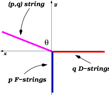
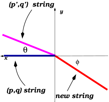
Figure 1: (1) On the Zero force condition on $q$ D-strings $\perp$ $p$ F-strings gives a $(p,q)$ string. (2) On the right a $(p,q)$ and $(p^{\prime},q^{\prime})$ string meet to form a new string – a $(p\pm p^{\prime},q\pm q^{\prime})$ string.

$$x: \mu_{(p,q)}\sin\theta=q\mu_{D1}=\frac{q}{2\pi\alpha^{\prime}g_{s}}$$

$$y: \mu_{(p,q)}\cos\theta=p\tau_{F1}=\frac{p}{2\pi\alpha^{\prime}}$$ (11)

which yield

$$\mu_{(p,q)}=\sqrt{(p\mu_{(1,0)})^{2}+(q\mu_{(0,1)})^{2}}=\frac{1}{2\pi\alpha^{\prime}}\sqrt{p^{2}+q^{2}/g_{s}^{2}}$$ (12)

Note, if the Ramond-Ramond scalar $A$ is nonzero there is a more general formula: $\mu_{(p,q)}=\mu_{F}[(p-Aq)^{2}+q^{2}/g_{s}^{2}]^{1/2}$. Note, for relatively prime $p$ and $q$ the triangle inequality ($|x|+|y|\geq|x+y|$) states that a $\mu_{(p,q)}<p\mu_{F1}+q\mu_{D1}$ as expected for a bound state.

More generally the force balance condition for a $(p_{i},q_{i})$ string vertex is $\sum_{i}\mu_{(p_{i},q_{i})}\hat{n}_{i}=0$, where $\hat{n}_{i}$ is the direction along which the $(p_{i},q_{i})$ string is aligned. The total charge entering and leaving a vertex must also be zero implying $\sum_{i}p_{i}=0$ and $\sum_{i}q_{i}=0$ at a vertex. This implies that when a $(p,q)$ string and a $(p^{\prime},q^{\prime})$ string meet, that either a $(p+p^{\prime},q+q^{\prime})$ string or a $(p-p^{\prime},q-q^{\prime})$ string will form.

Align the $(p,q)$ string along the $x$-axis and the $(p^{\prime},q^{\prime})$ string at an angle $\theta$ as in the right side of figure 1. The forces on the string junction are then

$$F_{x}(\theta,\phi) = \mu_{(p\pm p^{\prime},q\pm q^{\prime})}\cos\phi-\mu_{(p,q)}-\mu_{(p^{\prime},q^{\prime})}\cos\theta$$ (13)

$$F_{y}(\theta,\phi) = \mu_{(p^{\prime},q^{\prime})}\sin\theta-\mu_{(p\pm p^{\prime},q\pm q^{\prime})}\sin\phi$$ (14)

We now find the angle $\theta_{\pm}$ commensurate with $F_{x}=F_{y}=0$. After squaring both sides, then adding them together, and using $\mu_{(p\pm p^{\prime},q\pm q^{\prime})}^{2}=\mu_{(p,q)}^{2}+{\mu_{(p^{\prime},q^{\prime})}}^{2}\pm 2(pp^{\prime}+g_{s}^{-2}qq^{\prime})$ we find that the critical angles $\theta_{\pm}$ are

$$\cos\theta_{\pm}=\pm\frac{pp^{\prime}+g_{s}^{-2}qq^{\prime}}{\sqrt{p^{2}+g_{s}^{-2}q^{2}}\sqrt{p^{\prime 2}+g_{s}^{-2}q^{\prime 2}}}\equiv\pm\frac{{\mbox{\boldmath$\mu_{(p,q)}\cdot\mu_{(p^{\prime},q^{\prime})}$}}}{{\mbox{\boldmath$|\mu_{(p,q)}||\mu_{(p^{\prime},q^{\prime})}|$ }}}$$ (15)

where we have defined ${\mbox{\boldmath$\mu_{(p,q)}$}}=(p,g_{s}^{-1}q)$ and the inner product to be ${\mbox{\boldmath$\mu_{(p,q)}\cdot\mu_{(p^{\prime},q^{\prime})}$}}=pp^{\prime}+g_{s}^{-2}qq^{\prime}$ which implies ${\mbox{\boldmath$|\mu_{(p,q)}|$}}=\sqrt{p^{2}+g_{s}^{-2}q^{2}}$. Note, a configuration with both strings pointing towards the vertex and meeting at an angle $\theta_{+}$ is equivalent to a configuration where one string points in and the other points out of the vertex and where the intersection angle is $\theta_{-}=\pi-\theta_{+}$.

What happens when two strings meet and the angle is not $\theta_{+}$ or $\theta_{-}$? The intersection is not BPS and the strings will try to move to a BPS angle. If the heavier $(p+p^{\prime},q+q^{\prime})$ string instead of a $(p-p^{\prime},q-q^{\prime})$ is to form then the $(p,q)$ and$(p^{\prime},q^{\prime})$ strings should be closer together (in terms of the angle $\theta$) to balance the tension of the heavier $(p+p^{\prime},q+q^{\prime})$ string. If initially $\theta<\theta_{+}$, the vertex will move into the second quadrant of figure 1 and the $(p,q),(p^{\prime},q^{\prime})$ strings will curve so that near the vertex the angle $\theta$ grows to $\theta_{+}$ to make the vertex stable. A lighter $(p-p^{\prime},q-q^{\prime})$ string can only form if the strings are far enough apart to balance the lighter $(p-p^{\prime},q-q^{\prime})$ string. If suppose two strings (one pointing inwards and one pointing outwards) meet at an angle $\theta>\theta_{+}$. Then the lighter string can form if the vertex moves such that the two strings curve near the vertex to decrease $\theta$ to $\theta_{+}$.

2.4 Wrapped branes as 4D baryons

$(p,q)$ strings can end on branes which may be partially or completely wrapped on compact cycles. A completely wrapped brane looks like a heavy particle from a (3+1)D point of view and is sometimes called a baryon. At first glance this is confusing as the endpoints of strings are charged and charge conservation requires that a string ending on a brane must transfer its charge to the brane [47, 48, 49]. This in fact happens because the gauge invariant 2 form on the brane is not the electromagnetic field strength ${\cal{F}}_{2}=d{\cal{A}}_{1}$, but rather the combination ${\cal{F}}_{2}+B_{2}$. Thus if $B_{2}$ disappears on a brane (i.e an F-string ends on a brane) then a non-zero flux of ${\cal{F}}_{2}$ on the brane is produced. Also interestingly, if say $M$ units of $\int F_{3}$ flux threads a compact cycle ${\cal{K}}_{3}$ and a $D3$ brane wraps the cycle then charge conservation requires that $M$ F-strings end on the baryon. This effect arises because of the Chern-Simons term $\int_{D3}{\cal{F}}_{2}\wedge A_{2}$ on the brane which allows $F_{3}=dA_{2}$ to source ${\cal{F}}_{2}+B_{2}$.

The action of a brane + fundamental string is ignoring various constants including F-string and brane tensions

$$S = -\frac{1}{2}\int_{D3}|{\cal{F}}_{2}+B|^{2}-\frac{1}{2}\int_{{\cal{M}}}|H_{3}|^{2}+\int_{F1}B_{2}+\int_{D3}{\cal{F}}_{2}\wedge A_{2}$$ (16)

The first term comes from expanding the Born-Infeld action $\int\sqrt{\eta_{\mu\nu}+{\cal{F}}_{\mu\nu}+B_{\mu\nu}}$ of a $D3$ brane. In the second term $H_{3}$ is the field strength of the gauge field $B_{2}$ and the integral is over spacetime ${\cal{M}}$. The third term $\int_{F1}B_{2}$ is the analog of (2) for a string with a 2-form potential $B_{2}$ and can be converted to a 10D integral $\int_{{\cal{M}}}B\wedge*j$ by introducing a 2-form current $j$. In our notation * is the 10D Hodge duality operator, and $\star$ is the 4D Hodge duality operator. Thus $\int_{D3}|{\cal{F}}_{2}+B_{2}|^{2}\equiv\int({\cal{F}}_{2}+B_{2})\wedge\star({\cal{F}}_{2}+B_{2})$ and $\int_{{\cal{M}}}|H_{3}|^{2}\equiv\int H_{3}\wedge*H_{3}$. The last term is a Chern-Simons term which reduces to an analog of (2) for the $A_{2}$ gauge field if $\int{\cal{F}}_{2}\in{\mathbb{Z}}$. Then $\int{\cal{F}}\wedge A_{2}\sim\int A_{2}$. Essentially, an integral $\int{\cal{F}}_{2}$ induces D-string charge.

The variations of (16) with respect to $\delta B_{2}$ and $\delta{\cal{A}}_{1}$ where ${\cal{A}}_{1}$ is the gauge field of ${\cal{F}}_{2}=d{\cal{A}}_{1}$ are

$$\delta S_{\delta B} = -\int_{D3}\delta B_{2}\wedge\star\,({\cal{F}}_{2}+B_{2})+\int_{{\cal{M}}}\delta B_{2}\wedge d*H_{3}+\int_{{\cal{M}}}\delta B_{2}\wedge*j_{F1}$$ (17)

$$\delta S_{\delta{\cal{A}}} = -\int_{D3}\delta{\cal{A}}_{1}\wedge d\star({\cal{F}}_{2}+B_{2})+\int_{D3}\delta{\cal{A}}_{1}\wedge F_{3}$$ (18)

which give rise to the field equations

$$d*H_{3} = -*j_{F1}+\star{\cal{F}}_{2}\,\delta^{6}(x)+\star B_{2}\,\delta^{6}(x)\$$ (19)

$$d\star({\cal{F}}_{2}+B_{2}) = F_{3}$$ (20)

We next integrate the L.H.S of (19) over an $S^{8}$ which intersects the F-string at only a point. Then $\int_{S^{8}}d*H=0$ is the integral of a total derivative over a compact surface and vanishes. The $S^{8}$ intersects the $D3$ brane in a $S^{2}$. Suppose that $B_{2}=0$ on the brane. Then

$$Q_{F1} = \int_{S^{8}}*j_{F1}=\sum_{i}\int_{S_{i}^{2}}\star{\cal{F}}_{2}$$ (21)

where $S_{i}^{2}$ is the $S^{2}$ surrounding the endpoint of the $i$th string ending on the $D3$ brane. We sum over all string endpoints $i$ in (21).

Suppose the $D3$ brane wraps the compact 3-manifold ${\cal{K}}_{3}$. For mathematical convenience we introduce punctures at the places where the strings end on the ${\cal{K}}_{3}$. Then integrating (20) over the ${\cal{K}}_{3}$ and setting $B_{2}=0$ we find

$$\int_{{\cal{K}}_{3}}d\star{\cal{F}}_{2}=\sum_{i}\int_{S^{2}_{i}}\star{\cal{F}}_{2}=\int_{{\cal{K}}_{3}}F_{3}$$ (22)

Thus combining (21) and (22)

$$Q_{F1}=\int_{{\cal{K}}_{3}}F_{3}$$ (23)

.

Thus if $\int_{{\cal{K}}_{3}}F_{3}=M$, then $M$ F-strings must come out of the wrapped $D3$ brane baryon. One can analogously show that if $\int_{{\cal{K}}_{3}}H_{3}=K$ then $K$ D-strings must emerge from the baryon. For both $M$ and $K$ nonzero, a $(M,K)$ string or $M$ D-strings and $K$ F-strings must end on the baryon.

This also means that a $(p,q)$ string may break on a baryon. A $(p,q)$ string will enter the baryon and a $(p-M,q-K)$ string will exit the baryon if the $(p-M,q-K)$ string can suck enough energy out of the $(p,q)$ string for baryon pair production to occur. Suppose $K=0$. We can roughly argue that this will occur if the difference in energies of the $(p,q)$ and $(p-M,q)$ strings is positive: $\Delta E=E_{(p,q)}-E_{(p-M,q)}\sim\sqrt{p^{2}+q^{2}/g_{s}^{2}}-\sqrt{(p-M)^{2}+q^{2}/g_{s}^{2}}\propto 2p-M>0$. Here we have assumed the strings have roughly the same length so that the energy difference is measured by the difference in tensions. Thus, baryon production can only occur if

$$|p|\geq\frac{M}{2}\ \ \ \ \ \ \ \ |q|\geq\frac{M}{2}$$ (24)

where we have also generalized to the $K\neq 0$ case. See (80) for a more detailed explanation.

2.5 Making sense of long superstrings

Superstring theory possesses a single length scale $\ell_{s}=\sqrt{\alpha^{\prime}}$ which is related to the Planck scale by $\ell_{P}=g_{s}\ell_{s}$. Thus strings are typically of Planckian size. In order to grow a fundamental string one can wrap it on a very large compact cycle. The energy of the string is the tension, times the size of the cycle, times the number of times it winds the cycle $w$. For example if wrapped on a circle, $E=2\pi Rw\mu_{F}$. Such a string wrapped on a circle/torus is unexcited and its size solely comes from the winding energy. Another way to grow a string is to heavily excite it. Quantization of the string gives $m\sim\sqrt{N}$ where $N$ is the total excitation number of the string. Since $m=\mu_{F}\ell$ where $\ell$ is the length of the string, a highly excited string will have $\ell\sim\sqrt{N}$.

If the string is macroscopic then it can be described by a Brownian random walk, as each bit of a long string seems to act independently of other bits of the string. One can calculate the mean squared separation of two points on an open string as ${\cal{D}}^{2}=d\int\frac{d\sigma}{\pi}[X^{\mu}(0,\sigma+\Delta\sigma)-X^{\mu}(0,\sigma)]^{2}$. Here we have picked out some dimension $\mu$ among the $d$ spacetime dimensions and averaged over $\sigma$. Using the mode expansion for $X^{\mu}$ we can show that ${\cal{D}}^{2}\propto\Delta\sigma\propto\ell$ [50, 51, 52]. A Brownian random walk is characterized by the mean squared displacement between two points on the random walk curve satisfying $|\mbox{\boldmath$X$}_{1}-\mbox{\boldmath$X$}_{0}|^{2}\propto t_{1}-t_{0}$ where $(t_{1}-t_{0})$ is essentially the number of random walks steps taken from point $\mbox{\boldmath$X$}_{0}$ to get to point $\mbox{\boldmath$X$}_{1}$ if the time step is $\Delta t=1$. Hence, $(t_{1}-t_{0})$ is also the arclength $L$ of the random walk curve between $\mbox{\boldmath$X$}_{0}$ and $\mbox{\boldmath$X$}_{1}$ and therefore the random walk is characterized by $|\mbox{\boldmath$X$}_{1}-\mbox{\boldmath$X$}_{0}|^{2}\propto L$. Thus a long superstring with ${\cal{D}}^{2}\propto\ell$ can also be thought of as a random walk (with step size $\ell_{s}$ and number of steps $\sqrt{N}$).

Now cosmic strings can also be thought of as Brownian random walks [52, 53, 54], and thus it seems reasonable to identify fundamental cosmic superstrings as highly excited superstrings. Such strings can be thought of as classical correspondence limits (with mode number $N\rightarrow\infty$) of quantum strings. However, there are a number of issues associated with such highly excited strings. First, they naturally appear only at around the Hagedorn temperature which is not well understood. At such high densities long open strings soak up all the extra energy and tend to grow longer at the expense of smaller superstrings [50, 51, 52]. Second, although interactions are generally ignored, in the presence of gravity Hagedorn strings can encounter a Jeans instability [55].

In fact, one might worry that the self-gravity of such massive strings will cause them to collapse to black holes. A string can smoothly turn into a black hole only when its entropy $S_{string}$ matches the black hole entropy $S_{bh}$. However, the entropies match only at a critical string mass $m_{c}\sim m_{s}/g_{s}^{2}$. Above $m_{c}$ the string entropy $S_{string}\sim m$ is less than the black hole entropy $S_{bh}\sim m^{(D-1)/(D-2)}$ in $D$ spatial dimensions. Only, when $m$ decreases to $m_{c}$ will string self-gravity collapse a random walking string to a size equal to its Schwarzschild radius, which in this case is $\ell_{s}$ [56, 57, 58]. But, since $m\gg m_{c}$ for horizon-sized cosmic strings with $g_{s}\sim{\cal{O}}(10^{-1})$ we will not worry about this. A black hole can also form if a random walking cosmic string with say $G\mu_{F}\sim 10^{-7}$ random walks itself into a region less than its Schwarzschild radius $\sim\ell_{s}$. However, it would then have to double back on itself about $10^{7}$ times since the random walk step size is $\ell_{s}$ for a superstring. Furthermore, if the string is stretched by the cosmic expansion, then the step size will be stretched to the size of the horizon making black hole formation even more improbable [59].

The picture that was previously put forward for fundamental cosmic superstrings is that they form at very high densities at around the Hagedorn temperature as perhaps in tachyon condensation. Then as the universe expands and the temperature redshifts the energy density drops and instead of long strings being entropically favored, smaller loops become entropically favored. Hence, the long strings tend to discharge part of their lengths in loops. This allows the strings to scale and eventually around $\sim\!\!20\%$ of the string density ends up in loops as opposed to initially being $\sim\!\!100\%$ in long strings [52, 54].

The correspondence between a cosmic string and a D-string is more straight-forward. Since D-strings are topological defects they are naturally very long (infinite in flat space) and there is no problem in thinking about astrophysically large D-strings. In some sense, with respect to closed string interactions, one can even think of them as (non-normalizable) coherent states of the closed string raising operators $\alpha_{-n}^{\mu}$. For example, for the bosonic string by operating on the vacuum state $|0\rangle$ with an exponential of operators $\alpha_{-n}$, which excites mode $n$ of the string, we get a D-string.

$$|D1\rangle\sim\delta(x^{m})\left[\prod_{n=1}^{\infty}\exp\left({-\frac{1}{n}\alpha_{-n}^{\mu}S_{\mu\nu}\tilde{\alpha}_{-n}^{\nu}}\right)\right]|0\rangle$$ (25)

Where $S$ is a $D\times D$ matrix [60, 61, 44, 45]. As described in the next section they are dynamically formed in a relatively well understood tachyon condensation process.

Another way to think about the cosmic string and superstring correspondence is via the AdS-CFT correspondence. Cosmic strings are gauge theory solitons and stringy objects have a gauge theory description via the Ads-CFT correspondence [14, 15, 62]. For example the dynamics of a D-string are governed by a $U(1)$ gauge theory with 8 scalars. And in the Klebanov-Strassler geometry (to be discussed later), F-strings are described by confining flux tubes. D-strings appear as Abrikosov-Nielsen-Oleson vortices in an Abelian-Higgs system [63].

A different method of identifying gauge theory strings with D-strings has been the construction of Abrikosov-Nielson-Oleson vortices in $N=1,\,d=4$ super-Yang-Mills + gravity. In [64, 65], the authors tried to describe tachyon condensation using supergravity and the ensuing D-string creation using a $D$-term potential with a Fayet-Iliopoulos term. They identified the cosmic strings of the theory as D-strings in the low energy limit. If their identification is correct then it would provide a non-stringy (field theoretic) description of stringy objects and should be useful in examining the properties of stringy cosmic strings such as their stability, etc..

2.6 Cosmic string velocity

Finally, because we will continually invoke this result we prove as in [43, 54] that the mean square average velocity of a closed cosmic string in flat space is 1/2 and in expanding spacetime is $\leq 1/2$. Here we ignore the extra dimensions and write $X^{\mu}=(X^{0},\mbox{\boldmath$X$})$ where $X$ is the 3D string position vector.

We define $\langle v^{2}\rangle$ as

$$\langle v^{2}\rangle=\int_{0}^{T}\frac{dt}{T}\int_{0}^{L}\frac{d\sigma}{L}\mbox{\boldmath$\dot{X}$}^{2}$$ (26)

If we use the gauge conditions described in (134) and the equation of motion $\ddot{\mbox{\boldmath$X$}}=\mbox{\boldmath$X$}^{\prime\prime}$ and integrate by parts then we can write

$$\int d^{2}\sigma\mbox{\boldmath$\dot{X}$}^{2}=-\!\int d^{2}\sigma\mbox{\boldmath$X$}\!\cdot\!\ddot{\mbox{\boldmath$X$}}=-\!\int d^{2}\sigma\mbox{\boldmath$X$}\!\cdot\!\mbox{\boldmath$X$}^{\prime\prime}=\int d^{2}\sigma(\mbox{\boldmath$X$}^{\prime})^{2}=\int d^{2}\sigma(1-\mbox{\boldmath$\dot{X}$}^{2})$$ (27)

where the integral is over one string oscillation period and over the length of the string. Combining (26) and (27) we deduce that $\langle v^{2}\rangle=1/2$.

Now consider an expanding spacetime with scale factor $a$. If we differentiate the generalized version of (26) using the averaging in (124) and using the equation of motion of $X$ we can find an evolution equation for $v$:

$$\dot{v}=(1-v^{2})\left(\frac{k}{R}-2\frac{\dot{a}}{a}v\right)$$ (28)

where $k(v)$ is given by the phenomenological formula

$$k(v)=\frac{2\sqrt{2}}{\pi}\frac{1-8v^{6}}{1+8v^{6}}$$ (29)

.

Thus for $v=1/\sqrt{2}\Rightarrow k=0$ and from (28), $\dot{v}<0$. Thus in an expanding spacetime $v^{2}\leq 1/2$. This result also applies to $3+n$ spatial dimensions where the $n$ directions are fixed.

3 Dynamical production of D-branes

We have seen that D-branes are nonperturbative (in the sense that they cannot be obtained from the linearized field equations) solutions of the gravity + supersymmetry equations of motion. However, how does one dynamically produce a brane? Phase transitions are well known mechanisms for producing solitons as topological defects and are signalled by the presence of an unstable mode – a negative mass excitation, a tachyon. We thus look for controllable tachyonic string backgrounds.

3.1 Tachyon condensation at zero and finite temperature

Certain open string backgrounds are well known to be tachyonic because they are not supersymmetric. (They are often represented by coincident brane-antibrane pairs.) On these backgrounds, the tachyon field, $t$, possesses a potential $V(t)$ which depends on only $|t|$ and has a double well shape. Initially, the tachyon starts at the top of the potential $t=0$, and then rolls down to the bottom $t_{0}$. If no topological obstructions to tachyon condensation exist, then at the bottom of the well $t=t_{0}$, the negative tachyon energy cancels the energy of the open string background (the tensions of the brane and antibrane) leaving a closed string background populated with heavy closed fundamental strings as decay products. However, if topological obstructions exist then solitonic defects may also be produced.

In particular, if tachyon condensation in IIB string theory happens in $D_{t}$ spatial dimension, then branes with $D_{t}-2,D_{t}-4,D_{t}-6,...$ spatial dimensions may be produced as topological defects. A vortex with $p=D_{t}-2$ is the highest dimension D-brane that can be produced. It corresponds to $\pi_{1}({\cal{M}})\neq 0$ where ${\cal{M}}$ is the vacuum manifold of the tachyon potential. Hence if tachyon condensation occurs in only (3+1) dimensions, only D-strings and $D(-1)$ instantons may be produced.

How do we fit this into a cosmological scenario? We give two methods.

(1) If a brane collides with a parallel antibrane and forms a bound state, i.e. doesn’t simply pass through the antibrane – then a tachyonic background will form on the volume jointly occupied by the brane and antibrane. Most brane inflation mechanisms employ this scenario to create tachyons to create topological defects. A variant of this scheme is when two branes intersect each other in a “non-BPS” way. Tachyons appear at the intersection.

(2) Suppose the universe starts off in some non-supersymmetric open string state like a state with $N$ spacefilling brane-antibrane pairs. It will generally then be tachyonic at zero temperature. If the temperature is sufficiently high, finite temperature corrections may turn the negatively curved part of the tachyon potential into a positively humped part, thus removing the tachyon [66]. See figure 2. This will occur at temperatures above $T>T_{c}=T_{H}/\sqrt{g_{s}N}$, where $T_{H}$ is the Hagedorn temperature. Finite temperature effects shift the equilibrium value of the tachyon field upward – towards the symmetric point. This decreases the tachyon mass. Although, it costs energy to do this, a gas of smaller mass tachyons has a larger entropy. This phenomenon is familiar in finite temperature field theory where symmetry restoration results from finite temperature loop corrections [67].

Figure 2: The tachyon potential $V(t)$ above and below the critical temperature $T_{c}$ $\sim T_{H}/\sqrt{g_{s}N}$

However, if the universe is adiabatically expanding, for example expanding due to the positive vacuum energy of the $t=0$ vacuum state, the temperature will redshift and drop. Once it falls below $T_{c}$, a tachyon will develop dynamically and destabilize the space on which the tachyon field has support. The tachyon will then condense by rolling to the minimum of the potential which is characterized by the vacuum manifold ${\cal{M}}$ of the tachyon potential. On ${\cal{M}}$, $t$ will be characterized by a set of phase angles, $\{\theta_{i}\}$, and a modulus $|t_{0}|$. For example, if ${\cal{M}}=S^{1}$, the tachyon will receive the expectation value $\langle t\rangle=|t_{0}|e^{i\theta}$. However, near the temperature $T_{c}$, the tachyon field will randomly fluctuate, rolling down the potential and then rolling up via thermal fluctuations. Hence $t$ will not take on any definite values and the phase angles will fluctuate. Once the temperature falls below $T_{c}$ and reaches the Ginzburg temperature $T_{G}$, thermal fluctuations will no longer be able to push the tachyon up the potential again. At this point, once the tachyon rolls to the bottom of $V(t)$, its phase will be frozen in. Note, the Ginzburg temperature is close to $T_{c}$ and can be written as $h(g_{s})T_{c}$, where $h(g_{s})$ depends only on the string coupling and is typically close to unity [54].

3.2 D-string creation by the Kibble mechanism

In a second order phase transition such as the tachyonic transition, the correlation length of the field is very large. However, expanding universes have causal horizons which bound the distance over which causal processes can occur. In a universe with a Hubble parameter $H\sim 1/t$, causal processes can occur only within a sphere of diameter $H^{-1}$. Thus an expanding universe will have regions which are causally disconnected from each other.

Suppose that no topological obstructions to tachyon condensation exist. Then the tachyon field will have a magnitude $|t_{0}|$ everywhere. However, because Hubble volumes are causally disconnected and since the tachyon’s phase on ${\cal{M}}$ is randomly determined, the tachyon’s phase will generally be different in different Hubble volumes. Spacetime will thus possess a domain type structure, with the expectation value $\langle t\rangle$ varying from Hubble region to region in a relatively random way. The question answered by Kibble about cosmological phase transitions (like our tachyonic transition) was whether any residue of false vacuum remains anywhere. In particular can false vacuum be trapped at the intersection points of Hubble regions like flux tubes are trapped in a superconductor [68]? The answer is yes, but depends on the shapes of the Hubble regions, how they intersect and the number of expanding spatial dimensions $D_{e}$. In general since one intersection can roughly be associated to each Hubble volume, a lower bound on the number of branes formed by tachyon condensation in an expanding universe is: one brane per Hubble volume.

Figure 3: Three Hubble volume sized regions $A,B,C$, intersect at a point $P$, which is actually a 7D edge. The tachyon field takes the values $t_{A},t_{B},t_{C}$ on $A,B$ and $C$ respectively. The tachyon field maps the upper loop in spacetime, $D$, which encloses $P$ to the lower loop on the vacuum manifold, $E$, and is an element of $\pi_{1}({\cal{M}})$.

Suppose that all the directions that the tachyon has support on are expanding such that if $D_{e}$ is the number of expanding directions: $D_{t}=D_{e}$. Also, suppose that three cells meet along an edge as in figure 3. The edge is $D_{e}-2$ dimensional and coming out of the paper. The phase change around the closed curve $\gamma$ enclosing the edge at $P$ will be $2\pi$. The tachyon field, $t(\mbox{\boldmath$x$})$ maps $\gamma$ to the locus $\Gamma$ which winds ${\cal{M}}$ and is an element of $\pi_{1}({\cal{M}})={\mathbb{Z}}$. Conversely, non-triviality of $\pi_{1}({\cal{M}})$ implies that there exists a configuration, notably the 3 intersecting cells, for which a $S^{1}$ in spacetime can be mapped to a locus winding the vacuum manifold.

Attempts to shrink the curve in spacetime will cause the path $\Gamma$ to move off of ${\cal{M}}$ and upwards to the false vacuum $t=0$. Thus along the edge, which is the intersection of the cells, a line defect of false vacuum will be trapped. For a tachyon solely residing in the expanding $D_{e}$ dimensions this corresponds to a $(D_{e}-2)$-brane. For example, if the tachyon has support on 5 spatial dimensions the trapped false vacuum will correspond to a $D3$ brane – a braneworld. If $D_{e}\geq 5$ then $D3$ branes must form at intersections of more than three Hubble regions. For example, if nine dimensions expand then $D3$ branes will form at the intersections of 7 different Hubble regions. This is because the charge of a $D3$ brane is an integral of the five form field strength $F_{5}$ over an $S^{5}$: $Q_{D3}=\int_{S^{5}}*F_{5}$. An $S^{n}$ sphere is determined by $n+2$ points, and an $S^{5}$ is determined by seven points belonging to different Hubble volumes. Alternatively, the vacuum manifold in this case is ${\cal{M}}=U(2^{2})\sim S^{5}$. Hence a topological defect will exist if $\pi_{5}({\cal{M}})\neq 0$, which requires a mapping of an $S^{5}$ in spacetime to an $S^{5}$ on ${\cal{M}}$.

Suppose now that $D_{e}=3$ and that the number of spatial dimensions in which tachyon condensation occurs is $D_{t}=3+n$ and the $n$ dimensions are compact. Then only 3D regions lying along the expanding directions are causally separated. This trivial fact means that in 3+1 spacetime dimensions, the Kibble mechanism cannot populate the extra $n$ dimensions with topological defects. The Kibble mechanism will operate only in the expanding directions. I.e. the Kibble mechanism will produce only D-strings in large numbers. Monopole-like $D0$ branes or higher dimensional branes will not be Kibble produced.

For example, suppose tachyon condensation occurs in 7 spatial dimensions ($n=4$). Then $D5$ branes, $D3$ branes, D-strings and D-instantons may be produced. However, only D-strings, or objects which look like strings to a 4D observer will generically be mass produced by the Kibble mechanism. To produce a $D5$ brane two spatial dimensions of the 7D space must be cut away. If these two directions are in the expanding directions then one of the $D5$’s dimensions will be in the expanding directions and the other four directions of the $D5$ will be wrapped on a 4D compact cycle ${\cal{K}}_{4}$ and the Kibble mechanism can mass produce them. However, from a 4D point of view these $D5$ branes look like strings with a small thickness – which is their spread in the $n$ nonexpanding directions. See figure 4. $D3$ branes cannot be produced in large numbers because four dimensions of the 7D space must be cut away. Because there are only three expanding directions, one of those dimensions must be a nonexpanding direction. The Kibble mechanism cannot operate in that dimension, hence the Kibble mechanism will not produce 1 $D3$ brane/Hubble volume if $D_{e}\leq 3$. For $D3$ production $D_{e}$ must be at least 4, corresponding to a 4+1 dimensional expanding spacetime.

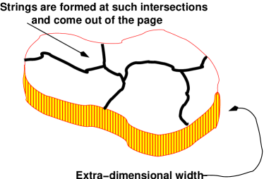
Figure 4: 4D strings formed at the intersections of different Hubble volumes may actually be higher dimensional branes wrapped on cycles in the extra dimensions. Their extra-dimensional part can be thought of as their 4D “thickness.”

4 Production of F and $(p,q)$ strings

We learned that open string tachyon condensation can lead to D-string production. We now show how the phase transition produces F-strings. Once F-strings and D-strings are produced collisions of $p$ F-strings and $q$ D-strings can produce $(p,q)$ string bound states as described in section $\S$2.3

4.1 F-strings as confining flux tubes

One argument put forward for the appearance of F-strings is the following. Suppose a $Dp-\bar{D}p$ brane anti-brane pair annihilate to form a lower dimensional $D(p-2)$ brane. A brane has a $U(1)$ gauge symmetry. Thus the gauge group of the brane-antibrane system consists of the two $U(1)$’s on each brane and is $U(1)\times U(1)$. The daughter brane possesses a $U(1)$ group which is identified as the linear combination $U(1)_{-}$ of the original two $U(1)$s. The other linear combination $U(1)_{+}$ must disappear because only one brane remains. The $U(1)_{+}$ is thought to disappear by having its fluxes confined by confining strings which are thought to be F-strings.

4.2 Closed string production using boundary CFT

A more technical argument which produces closed strings and should carry over to open string production goes as follows. Tachyons cause the production of D-strings and F-strings. Thus we should understand how perturbations due to tachyons change the string worldsheet action. Perturbations due to tachyons $t(X)$ and open string fields like $A_{\mu}$ can be calculated by adding to the action a deformation $\delta S(t,A_{\mu})$. The deformation must preserve conformal invariance. Deformations preserving scale invariance are by definition called marginal. A suitable marginal deformation is

$$\delta S=\int_{\partial D^{2}}ds\biggr{[}t(X(\sigma))+\partial X^{\mu}(\sigma)A_{\mu}(X(\sigma))+\cdots\biggr{]}$$ (30)

where the integration is over the boundary of the disk $\partial D^{2}$ which is parameterized by $s$.

We are only interested in the effects of the tachyon $t(X)$ and thus will set $A_{\mu}=0$. The linearized string field theory equation of motion for the tachyon is $(\partial^{2}-m^{2})t(X)=0$, [69, 70]. For spatially homogeneous tachyons it is satisfied by

$$t(X)=Ae^{-X^{0}}+Be^{X^{0}}$$ (31)

where we have set $m^{2}=-1$. For the boundary conditions $t(X^{0}=0)=\lambda$ and $\dot{t}(X^{0}=0)=0$ (31) gives

$$\delta S=\frac{\lambda}{2}\int_{\partial D^{2}}dse^{X^{0}}$$ (32)

$\lambda/2$ measures the strength of the perturbation; it need not be small.

Particle production in field theory can be described by an interaction $\int\!J(x)\phi(x)$ where the source $J(x)$ satisfies $(\partial^{2}-m^{2})\phi(x)=J(x)$ . For example, the source $J=g\chi\chi^{*}$ corresponds to an interaction like $g\chi\chi^{*}\phi$. In analogy, brane annihilation will produce closed strings because D-branes source closed strings. The source $J_{s}$ which couples to a closed string state $|\phi_{s}\rangle$ is the overlap $J_{s}=\langle\phi_{s}|J\rangle$ (up to multiplication by ghosts). Up to multiplication by ghosts, $|J\rangle$ is the boundary state $|J\rangle\sim|Dp\rangle$ representing the $Dp$-brane, which is the $Dp$ version of (25). The analogous Klein-Gordon equation is then

$$(\partial^{2}-m^{2}_{s})\phi_{s}=J_{s}$$ (33)

The task thus boils down to calculating the source $J_{s}=\langle\phi_{s}|Dp\rangle$. The state $\langle\phi_{s}|$ can be created from the vacuum by the (vertex) operator $V_{s}$ as $\langle\phi_{s}|=\langle 0|V_{s}$. Thus the item to calculate becomes

$$J_{s}=\langle 0|V_{s}|Dp\rangle_{S+\delta S}$$ (34)

where we have made explicit that the overlap is to be calculated with the modified action $S+\delta S$.

The number density of emitted closed strings and their average energy can be calculated as

$$\frac{N}{V}=\int\frac{dE}{2E}\rho(E)|J_{s}|^{2};\;\;\;\;\;\;\frac{E}{V}=\int\frac{dE}{2E}\cdot E\cdot\rho(E)|J_{s}|^{2}$$ (35)

where $\rho(E)$ is the density of string states. $N/V$ and $E/V$ diverge unless gravitational backreaction of daughter strings is taken into account [40, 71, 72]. Unfortunately taking backreation into account has been possible only in 2D string theory where gravity is much more benign [73, 74, 75]. Therefore we do not present the explicit calculation of (34). Nevertheless, as $N/V$ and $E/V$ are non-zero, we expect that fundamental strings are produced by tachyon condensation/brane-anti-brane annihilation.

4.3 How long are the F-strings?

The fundamental strings which are produced are long heavy strings much like field theory cosmic strings. The density of states $\rho(E)$ of a string grows exponentially with the mass as $\rho(m)\sim m^{a}e^{\alpha^{\prime}m}$ [76]. Thus the number of available massive states far outnumbers the number of low mass states. Note that an $|out\rangle$ state with a $\int J\phi$ interaction term is

$$|{\rm out}\rangle=Te^{-i\int H_{I}(t)}|{\rm in}\rangle=Te^{-i\sum_{s}\int\rho(s)J_{s}\phi_{s}}|{\rm in}\rangle\sim\sum_{n,m}(\rho J_{s})^{n}(a^{\dagger}_{s})^{n}|{\rm in}\rangle+\cdots$$ (36)

On the R.H.S. we used the quantization $\phi\sim\sum_{m}f_{s}a_{s}+f^{*}_{s}a^{\dagger}_{s}$. For point particle theories the $J^{n}(a^{\dagger}_{s})^{n}|{\rm in}\rangle$ components of the final state correspond to a final state with $n$ particles. However, in string theory $a^{\dagger}_{s}$ corresponds to the mode operator $\alpha_{(s<0)}^{\mu}$ which instead of creating strings, excites massive modes. Now $J_{s}$ is expected to fall exponentially with energy while $\rho$ rises exponentially with energy [40]. If $\rho$ wins or if $\rho J_{s}$ is not steeply suppressed tachyon condensation will lead to very massive strings.

The liberated energy density from $Dp$ brane annihilation is $\Delta\rho\sim(2\pi)^{-p}g_{s}^{-1}$ in string units. Now, the Hagedorn energy density $\rho_{H}$ is approximately $\sim 1$ in string units [77, 78]. Thus for $g_{s}<1$, $\Delta\rho\sim\rho_{H}$. In the Hagedorn regime long strings are predominant. This provides another hint that long strings are produced.

We can estimate the length of the F-strings as follows. A $Dp$-brane is expected to decay inhomogeneously to $D0$ branes and then to closed strings [40]. A $D0$-brane has an energy $E_{D0}=m_{s}/g_{s}$. If each $D0$ decays to a single string, the length of the string would be $\ell=E_{D0}/\mu_{F}$. Using $g_{s}=0.1$, we find $\ell=60\ell_{s}$. If however clusters of say $10^{8}$ D-particles condense to form one F-string then instead $\ell\approx 10^{10}\ell_{s}$. This would compare quite favorably with the horizon size $\ell_{H}$ at the brane inflation energy scale $m_{inf}$ since $\ell_{H}\sim(\frac{m_{P}}{m_{inf}})^{2}\ell_{P}$ [79]. (The Friedmann equation gives $t\sim m_{P}/T^{2}$ where the temperature scales as $T\sim m_{inf}$.) If $m_{inf}\approx 10^{-4}m_{P}$ as in the KKLMMT model and $\ell_{p}\sim\ell_{s}$ then the length of such strings is around the size of the horizon, $\ell\sim\ell_{H}$ and they are effectively infinite.

5 How to make cosmologically viable cosmic superstrings

If the string scale mass $m_{s}\equiv 1/\sqrt{\alpha^{\prime}}$ is of order the Planck mass $m_{P}$ and $g_{s}$ is not very small (say $g_{s}\sim 1/4$), then the four dimensional F and D string self gravity is $G_{4}\mu_{F}\sim{\cal{O}}(g_{s}^{2})$ and $G_{4}\mu_{D1}\sim{\cal{O}}(g_{s})$. However, current cosmic microwave background measurements have placed an upper bound on the self gravity of line-like defects of $G\mu<10^{-6}$. Thus, without new ideas, networks of cosmic sized F or D strings are thought to be unrealistic.

5.1 Warped geometries suppress the string tension

As is now familiar from the Randall Sundrum story one way to make superstrings much lighter is to make the 4D constants dependent on the extra dimensions [37, 38]. An innocuous way to do this is by warping the 4D metric as follows

$$ds^{2}=G_{MN}dx^{M}dx^{N}=e^{2A(y)}g_{\mu\nu}(x)dx^{\mu}dx^{\nu}+e^{-2A(y)}\tilde{g}_{mn}(y)dy^{m}dy^{n}$$ (37)

where $g_{\mu\nu}(x),\tilde{g}_{mn}(y)$ are the metrics of the 4 large dimensions $x^{\mu}$, and the 6 extra dimensions $x^{m}$ respectively. The four dimensional warp factor is $e^{2A(y)}$. The measure factor $\sqrt{|G_{MN}|}$ in the action then breaks up as $\sqrt{|G_{MN}|}=e^{-2A(y)}\sqrt{|g(x)|}\cdot\sqrt{|\tilde{g}(y)|}$. We then integrate over $y$. Then $m_{P}^{2}$ in $S=m_{P}^{2}\int\sqrt{|G|}d^{10}x(R+\cdots)$ becomes $m_{P}^{2}\int d^{6}ye^{-2A(y)}\sqrt{|\tilde{g}(y)|}\approx m_{P}^{2}$ if $A(y)$ is linear in $y$ and $\sqrt{|\tilde{g}(y)|}\sim{\cal{O}}(1)$. Thus warping doesn’t appreciably change the four dimensional metric determinant. However, warping changes the 4D metric from $g_{\mu\nu}$ to $e^{2A(y)}g_{\mu\nu}$. Thus quantities depending on the metric like the energy momentum tensor $T_{\mu\nu}$ for a domain wall/brane/D-string change as [22]

$$T_{\mu\nu}=-\mu_{D1}g_{\mu\nu}\delta^{8}(x,y)\quad\Longrightarrow\quad-\mu_{D1}e^{2A(y)}g_{\mu\nu}\delta^{8}(x,y)$$ (38)

We see that the tension is redshifted by the factor $e^{2A(y)}$. At certain points $\{y^{m}\}$ on certain compact manifolds we can engineer $A\sim-9$. At such points the tension of a F or D string is reduced to

$$\mu_{(p,q)}\simeq 10^{-8}m_{p}^{2}\ \ \ \ \Longrightarrow \ \ \ G_{4}\mu_{(p,q)}\sim 10^{-8}$$ (39)

Such large redshifts can occur at the bottom of a gravitational potential like a throat in a compact manifold, see figure 5.

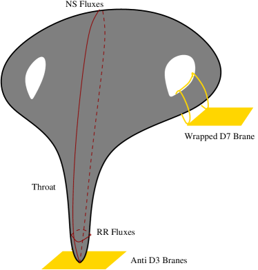
Figure 5: A finite throat is “attached” to a 6D Calabi-Yau. Branes or antibranes can sit at the bottom of the throat, and other branes like $D7$’s can wrap other cycles of the CY. (From [80].)

Manifolds with throats like these can be engineered in a variety of ways. We now give several examples.

5.2 Warped example 1: Anti-de Sitter Space

Anti de Sitter space has large warping near $r\sim 0$ [14, 45]

$$ds^{2}_{AdS}=\frac{r^{2}}{R^{2}}(-dt^{2}+d\vec{x}^{2})+\frac{R^{2}}{r^{2}}dr^{2}$$ (40)

where $R$ is the curvature radius of AdS. The standard Randall Sundrum approach uses this space and cuts off AdS at some $r_{0}$ and $r_{max}$, such that $r_{0}<r<r_{max}$. The cutoff is performed by placing a brane at $r_{0}$ – the ”standard model” brane, and by placing a brane at $r_{max}$ – the ”Planck brane.” Mass scales on the standard model brane are severely redshifted by $(\frac{r_{0}}{R})^{2}\ll 1$.

5.3 Warped example 2: near horizon limit of coincident branes

Earlier we wrote down the metric of a $D1$ brane in (6). $N$ coincident extremal (i.e. supersymmetric) D3-branes have a similar looking metric [45, 7]

$$ds^{2} = h(r)^{-1/2}(-dt^{2}+dx_{i}dx^{i})+h(r)^{1/2}(dr^{2}+r^{2}d\Omega_{8-p})$$

$$h(r) = 1+\frac{4\pi Ng_{s}\alpha^{\prime 2}}{r^{4}}$$ (41)

We can study the small $r$ region of (41) by taking the “near horizon limit.” This is obtained by taking the $\alpha^{\prime}\rightarrow 0$ limit (which decouples the brane from the bulk) while scaling $r$ at the same time such that the variable $u\equiv r/\alpha^{\prime}$ is meaningful. If we regard $r$ as the distance between parallel branes the mass of the strings connecting the branes is $u$ which also controls the values of gauge theory quantities on the brane like the expectation value of the Higgs. Thus the latter condition keeps the mass of these strings and Higgs vevs finite as the branes become coincident at $r=0$.

In this limit as $r\rightarrow 0$ we can drop the ”1+” in the harmonic function $h(r)$. The $N$ D3 branes’ metric then becomes warped AdS times a sphere $S^{5}$. In the new coordinate $u$ the $N$ coincident $D3$s’ metric is

$$\frac{ds^{2}}{\alpha^{\prime}}=\frac{u^{2}}{L^{2}}(-dt^{2}+dx_{i}dx^{i})+\frac{L^{2}}{u^{2}}(du^{2}+u^{2}d\Omega_{5}^{2}).$$ (42)

The radius of the sphere in string units is $L=(4\pi Ng_{s})^{1/4}$.

The massive warping as $u\rightarrow 0$ means the brane sits at the bottom of an infinite throat and all energies are infinitely redshifted there, see figure 6. Chan, Paul and Verlinde (CPV) and others implemented this model in a real compactification [81]. CPV placed a brane at a point on a compact Calabi-Yau. From the point of view of the transverse directions, near the brane a semi-infinite throat appears off the Calabi-Yau, see figure 5.

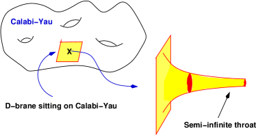
Figure 6: A brane sits on the Calabi-Yau at X. A semi-infinite throat branches off at X.

However, this model is unsatisfactory because one would like a finite throat producing severe but finite warping. Also, in the CPV model, the D3 brane could be anywhere. No potential fixing its position on the Calabi-Yau appears. This adds arbitrariness to the model.

5.4 Warped example 3: flux compactifications

Giddings, Kachru and Polchinski (GKP) attempted to fix the problems of the Verlinde model by transplanting a result of Klebanov and Strassler (KS) into the Verlinde model. Klebanov and Strassler showed how to produce heavily warped finite throats. Specifically, they showed that if certain compact cycles, notably $S^{3}$’s and $S^{2}$’s, degenerated at certain points, some of those cycles could be blown back up by threading flux through the cycles. The geometry near the resolved singular points is warped and the throat resulting from the warping is finite. The fluxes act as a positive pressure expanding the degenerating cycles and reduce the amount of supersymmetry. They also generate a potential for various scalar fields which parameterize the size and shape of the compact manifold.

5.4.1 The conifold and resolution of its conic singularity

A conifold is a singular manifold which is topologically a cone and is an $S^{3}\times S^{2}$. It becomes singular because the $S^{3}$ and $S^{2}$ shrink to zero size [82, 83, 44, 84]. See figure 7. If the singularity is desingularized by blowing up the $S^{3}$ it becomes a deformed conifold.

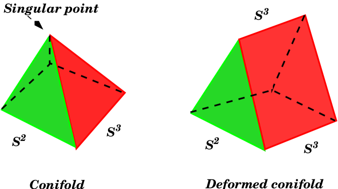
Figure 7: A conifold can be de-singularized by blowing up the $S^{3}$. The new space is the deformed conifold.

Conifold singularities are the most generic singularities in Calabi Yau compactifications. Calabi-Yau manifolds are often defined by complex algebraic curves like $f(w_{1},...,w_{4})=0$. The conifold is singular because $\partial_{w_{i}}f(w_{1},...,w_{4})=0$ for all $i$. However, it is not “that singular” because the matrix of second derivatives is nonzero, $\partial_{w_{i}}\partial_{w_{j}}f(w_{1},...,w_{4})\neq 0$. Near the singularity $f(w_{1},...,w_{4})$ can be written as

$$f(w_{1},w_{2},w_{3},w_{4})=w_{1}^{2}+w_{2}^{2}+w_{3}^{2}+w_{4}^{2}=0$$ (43)

.

The origin (0,0,0,0) is singular. Note (43) defines a 6D manifold and is a cone because if $w$ is on the conifold then so is $\lambda{\mbox{\boldmath$w$}}$ for $\lambda\in{\mathbb{C}}$. To understand what the base of the cone looks like, we first write the $w_{i}$ in terms of real coordinates $w_{i}=x_{i}+iy_{i}$. Equation (43) becomes ${\mbox{\boldmath$x$}}^{2}-{\mbox{\boldmath$y$}}^{2}=0$ and ${\mbox{\boldmath$x$}}\cdot{\mbox{\boldmath$y$}}=0$. We then intersect (43) with a 7-sphere centered at the apex of the cone: $|w_{1}|^{2}+\cdots+|w_{4}|^{2}=r^{2}$ which is equivalent to ${\mbox{\boldmath$x$}}^{2}+{\mbox{\boldmath$y$}}^{2}=r^{2}$. At the intersection of $f(w_{1},w_{2},w_{3},w_{4})$ and the $S^{7}$ we find

$$x_{1}^{2}+x_{2}^{2}+x_{3}^{2}+x_{4}^{2}=\frac{r^{2}}{2}\;\; x\cdot y=0 \;\;y_{1}^{2}+y_{2}^{2}+y_{3}^{2}+y_{4}^{2}=\frac{r^{2}}{2}$$ (44)

The first of these defines an $S^{3}$. The second defines a surface through $(x,y)$ space, implying $y$ is orthogonal to $x$, or equivalently that $\{y\}$ is the coordinate of a fiber over the base spanned by $\{x\}$. The last equation defines an $S^{3}$. However the plane $x\cdot y$ slices the $S^{3}$, picking out an $S^{2}$. Thus (43) describes an $S^{2}$ fiber over an $S^{3}$. However, a useful fact is that all such bundles over $S^{3}$ are trivial [82]. Thus the bundle is globally a product and the conifold is simply an $S^{3}\times S^{2}$, as shown in figure 7.

Suppose we now deform the conifold by a real parameter $z$.

$$f(w_{1},w_{2},w_{3},w_{4})=z.$$ (45)

Then $z$ controls the size of the $S^{3}$ cycle which we denote by $A$. $z$ can be defined by the integral of an analytic function $\Omega$ with 3 indices (better known as the holomorphic 3-form) over the $A$ cycle

$$z=\int_{A}\Omega$$ (46)

Thus $z$ vanishes when the $S^{3}$ cycle $A$ vanishes. Turning on a finite $z$ turns the singular conifold into the less singular deformed conifold [44, 85].

When defining a basis of 3-cycles, we can restrict ourselves to non-intersecting cycles $A_{I}$ and cycles called $B_{I}$ which intersect $A_{I}$ once such that $A_{I}\cap B_{J}=\delta_{IJ}$. Note the $B_{J}$ are nonintersecting, $B_{J}\cap B_{K}=0$. In this case with a single $A$ cycle, a basis of 3-cycles spanning the 6D extra-dimensional space ${\cal{M}}_{6}$ is formed by an $A$ cycle and a $B$ cycle which intersects $A$ once. The $B$ cycle defines a coordinate $G$ conjugate to $z$

$$G=\int_{B}\Omega$$ (47)

If we go around the singularity $z=0$ in a circle there is no reason to expect that $G$ should return to itself, $G\rightarrow G$. In fact if we go around the singularity along the curve $B$ we actually end up traversing the curve $B+A$. Hence,

$$G\rightarrow G+z$$ (48)

Such behavior can be mimicked by

$$G=\int_{B}\Omega=\frac{z}{2\pi i}\ln z+\cdots{\rm nonsingular\,terms}$$ (49)

The branch cut of the log means

$$G\rightarrow\frac{z}{2\pi i}\ln z+\frac{z}{2\pi i}\cdot 2\pi i=G+z$$ (50)

as desired if $z=|z|\exp{(i\phi)}\rightarrow|z|\exp{i(\phi+2\pi)}$.

5.4.2 Calculation of the warp factor of the deformed conifold

The superpotential, from which the scalar potential emerges, is the integral of the three form $G_{3}=F_{3}-\tau H_{3}$ over ${\cal{M}}_{6}$ [22]. As usual, $\tau$ is the dilaton-axion in (9), $F_{3}$ is a 3-form field strength for D-strings and $H_{3}$ is the 3-form field strength for fundamental strings.

$$W = \int_{{\cal{M}}_{6}}(F_{3}-\tau H_{3})\wedge\Omega$$ (51)

$$= \left(\int_{A}F_{3}\right)\wedge\left(\int_{B}\Omega\right)+\left(\int_{B}\tau H_{3}\right)\wedge\left(\int_{A}\Omega\right)$$

Note the sign change $\int_{A}\wedge\int_{B}=-\int_{B}\wedge\int_{A}$. Suppose we place $M$ units of $F_{3}$ flux on the $A$ cycle and $-K$ units of $H_{3}$ flux on the $B$ cycle such that

$$\frac{1}{2\pi\alpha^{\prime}}\int_{A}F_{3}=2\pi M \frac{1}{2\pi\alpha^{\prime}}\int_{B}H_{3}=-2\pi K$$ (52)

Plugging (52) and the definitions of $z$ and $G$ into (51), the superpotential becomes

$$W=(2\pi)^{2}\alpha^{\prime}(MG-K\tau z)$$ (53)

Thus a nonzero superpotential and nonzero flux quanta $M,K$ can deform the conifold by turning on a finite deformation parameter $z$.

Supersymmetry requires that the ground state energy be zero. The scalar potential, $V$ is proportional to $(D_{z}W)^{2}$, where $D_{z}$ is the covariant derivative, $D_{z}=\partial_{z}+\partial_{z}{\cal{K}}$. Here ${\cal{K}}$ is the so-called Kahler potential and will be irrelevant here because $\partial_{z}{\cal{K}}$ is much smaller than the other terms near the conifold point $z\sim 0$ [86]. Thus using $\tau=i/g_{s}+\cdots$

$$0=\sqrt{V}\sim D_{z}W\sim\frac{M}{2\pi i}\ln z-i\frac{K}{g_{s}}+{\cal{O}}(1)$$ (54)

which yields

$$z\sim e^{-\frac{2\pi K}{Mg_{s}}}$$ (55)

We can now estimate the warp factor $e^{2A}$. The $H_{3}$ and $F_{3}$ fluxes can be related to $D3$ brane charge by $Q_{D3}\sim-\int H_{3}\wedge F_{3}$. Thus the threading of flux through the $A$ and $B$ cycles can equivalently be thought of as the positioning of $N=MK$ $D3$ branes at the bottom of the conifold throat. The warping can then by thought of as due to $N$ $D3$ branes just as in (42) but with distance to the branes $r$ cut off at some minimum (because of the resolution of the conifold singularity). The warping due to the branes $\sim 1/\sqrt{h(r)}\sim r^{2}$, is then equivalent to some $e^{2A}$ warp factor $\grave{a}$ $la$ the flat space version of (37). It turns out that $r$ is related to the conifold coordinates $|{\mbox{\boldmath$w$}}|$ as $r\sim|{\mbox{\boldmath$w$}}|^{2/3}$. Our resolution of the conifold singularity cuts the conifold off at $w_{i}^{2}\sim z$. Thus the minimum value of the warp factor is

$$e^{2A}|_{conifold\,\,tip}\sim r^{2}\sim|{\mbox{\boldmath$w$}}|^{4/3}\sim z^{2/3}\sim e^{-\frac{4\pi K}{3Mg_{s}}}$$ (56)

For reasonable values of $K$ and $M$ and $g_{s}$, a suppression of the string tension by at least $10^{-8}$ is possible.

One important point to note is that there is a minimum value of $M$ if brane-antibrane annihilation at the bottom of the conifold throat is to occur and produce $(p,q)$ strings. It was shown in [87] that unless

$$M\mathrel{\hbox to0.0pt{\lower 4.0pt\hbox{\hskip 1.0pt$\sim$}\hss}\raise 1.0pt\hbox{$>$}}12$$ (57)

that a antibrane part of the brane-antibrane pair at the end of the throat would be unstable and dissolve into flux. Thus if $M<12$ there would be no brane-antibrane pair whose annihilation would produce $(p,q)$ strings.

5.5 Why do warped models require orientifolds?

Orientifolds are unfamiliar objects to cosmologists. They are fixed planes of negative tension and hence are admittedly, bizarre. Below, without explaining why they are reasonable objects to work with, we review GKP’s argument of why they are generically required by warped compactifications.

The relevant part of the Type IIB supergravity action is

$$S_{IIB}=\frac{1}{2\kappa_{10}^{2}}\int d^{10}x\sqrt{|g|}\left(R-\frac{\partial_{M}\tau\partial^{M}\bar{\tau}}{2({\rm Im}\;\tau)^{2}}-\frac{|G_{3}|^{2}}{12\;{\rm Im}\;\tau}-\frac{|\tilde{F}_{5}|^{2}}{4\cdot 5!}\right)+S_{CS}+S_{loc}$$ (58)

Conceptually the above action is very similar to (4). However we have written it in the Einstein frame. We have added the F-string field strength $H_{3}$, 5-form field strength $F_{5}$ of $D3$ branes, and the D-instanton field strength $\partial A$ and combined all of the fields in a very elegant SL($2,{\mathbb{Z}}$) way [44]. A price of this elegance is that Im$\,\tau$ appears in the denominator of 2 terms. Here $S_{CS}$ is the Chern-Simons part of the action and $S_{loc}$ is the local part due to the presence of matter sources like branes, orientifold planes, etc.

In (58), $|G_{3}|^{2}$ means $G_{3}\wedge*G_{3}$. Also in (58) $\tilde{F}_{5}$ is self-dual, $\tilde{F}_{5}=*\tilde{F}_{5}$, and is defined by $\tilde{F}_{5}=F_{5}-\frac{1}{2}A_{2}\wedge H_{3}+\frac{1}{2}B_{2}\wedge F_{3}$. An ansatz for $\tilde{F}_{5}$ satisfying the Bianchi identity and self-duality is $\tilde{F}_{5}=(1+*)d\alpha\wedge dx^{0}\wedge dx^{1}\wedge dx^{2}\wedge dx^{3}$. Here $\alpha$ is a scalar function on the compact space.

The trace-reversed Einstein equation is

$$R_{MN}=\kappa_{10}^{2}\left(T_{MN}-\frac{1}{8}g_{MN}T\right)$$ (59)

Recall that $M,N$ are the 10D indices, $\mu,\nu$ are the noncompact indices and $m,n$ are the compact directions’ indices. The noncompact part of the R.H.S. of (59) is

$$T_{\mu\nu}-\frac{1}{8}g_{\mu\nu}T=-g_{\mu\nu}\left(\frac{G_{mnp}\bar{G}^{mnp}}{48{\rm Im}\tau}-\frac{e^{-8A}}{4}\partial_{m}\alpha\partial^{m}\alpha\right)+\kappa_{10}^{2}\left(T_{\mu\nu}^{loc}-\frac{1}{8}g_{\mu\nu}T^{loc}\right)$$ (60)

The Ricci scalar, $R_{\mu\nu}$ for the warped compactification (37) is

$$R_{\mu\nu}=-\eta_{\mu\nu}e^{4A}\tilde{\nabla}^{2}A.$$ (61)

Thus,

$$\tilde{\nabla}^{2}A=e^{-2A}\frac{G_{mnp}\bar{G}^{mnp}}{48{\rm Im}\tau}+\frac{e^{-6A}}{4}\partial_{m}\alpha\partial^{m}\alpha+\frac{\kappa_{10}^{2}}{8}e^{-2A}(T_{m}^{m}-T_{\mu}^{\mu})$$ (62)

If we integrate the above equation over the compact manifold ${\cal{M}}_{6}$, then the left hand vanishes because it is a total derivative. The right side apart from the last term is positive semi-definite. Thus for a nonvanishing warp factor $A$, the only way of matching both sides of (62) is if $T_{m}^{m}-T_{\mu}^{\mu}<0$. Now using (38), if $T^{loc}$ originates from $Dp$ branes which fill the four non-compact directions and wrap a cycle $\Sigma$ composed of $p-3$ compact directions, then

$$T^{loc}_{\mu\nu} = -e^{2A}T_{p}g_{\mu\nu}\delta(\Sigma)\;\;\Rightarrow\;\;T_{\mu}^{\mu}=-4T_{p}\delta(\Sigma)$$

$$T^{loc}_{mn} = -\Pi_{mn}^{\Sigma}T_{p}\delta(\Sigma)\;\;\ \ \;\Rightarrow\;\;T_{m}^{m}=-(p-3)T_{p}\delta(\Sigma)$$ (63)

Here $\Pi_{mn}^{\Sigma}$ is the projection of the compact directions’ metric $e^{-2A}\tilde{g}_{mn}$ onto the directions spanned by $\Sigma$. Thus,

$$0=\int\tilde{\nabla}^{2}A={\rm positive\;terms}+(7-p)T_{p}$$ (64)

If $p<7$ then the only way to satisfy (64) is if $T_{p}<0$. Thus negative tension objects like O3 planes are generically required by warped compactifications.

5.6 Consequences of orientifolds: unstable F and D strings

The closed string field $X^{\mu}$ can be decomposed into a right-moving part $X_{+}$ with worldsheet coordinate $\sigma_{+}$ and a left-moving part $X_{-}$ with worldsheet coordinate $\sigma_{-}$. Thus $X^{\mu}(\sigma_{+},\sigma_{-})=X_{+}(\sigma_{+})+X_{-}(\sigma_{-})$. A worldsheet parity operation $\sigma_{+}\leftrightarrow\sigma_{-}$, which is mediated by the operator $\Omega$ exchanges the right and the left-moving parts and is a symmetry of bosonic and Type IIB string theory because both are right-left symmetric. When this symmetry is combined with a spacetime symmetry like a spacetime reflection $R$ taking $X^{\mu}\rightarrow-X^{\mu}$, then at the fixed points of the combined world sheet parity $\times$ spacetime symmetry, we find solitonic kink-like objects. A scattering calculation shows that they have negative tension and are not dynamical. These are known as orientifold fixed planes. For example, in 10D string theory, if $X^{9}$ is noncompact and we identify by the ${\mathbb{Z}}_{2}$ symmetry, $X^{9}\cong-X^{9}$, then a 8D domain wall orientifold will be located at $X^{9}=0$. A string at positive $X^{9}$ will be identified with an orientation-reversed string at negative $X^{9}$. This general reflection property of orientifolded string theories implies that there is a mirrored reflection of every string or brane. In also means for example, that if a geometry has a throat like the conifold warped throat, that there exists a mirror throat. Thus if there exist strings and D-strings sitting at the bottom of a conifold throat, then there exist mirror states – strings with opposite orientation and anti-D-strings sitting at the bottom of a mirror conifold throat.

In supersymmetric theories the orientifold projection $R\Omega$ is modified by fermions to $R\Omega(-1)^{F_{L}}$. $F_{L}$ is the fermion number of left-handed fermions. Thus $R\Omega(-1)^{F_{L}}$ projects onto states with an even number of left-handed fermions.

$\Omega$ will project out various massless string modes. Left-handed level-1 creation operators are denoted by $\alpha^{\mu}_{-1}$ and right-handed level-1 creation operators by $\tilde{\alpha}^{\nu}_{-1}$. Then we can form the string state $B_{\mu\nu}\alpha^{\mu}_{-1}\tilde{\alpha}^{\nu}_{-1}|0\rangle$ where $B_{\mu\nu}$ is the F-string antisymmetric gauge field. Then under worldsheet parity, ${\sf right}\leftrightarrow{\sf left}$ exchanging $\tilde{\alpha}^{\nu}_{-1}\leftrightarrow\alpha^{\nu}_{-1}$. But $B_{\mu\nu}$ is antisymmetric under $\mu\leftrightarrow\nu$ and thus the state’s $\Omega$ eigenvalue is -1:

$$\Omega:B_{\mu\nu}\alpha^{\mu}_{-1}\tilde{\alpha}^{\nu}_{-1}|0\rangle\rightarrow-B_{\mu\nu}\alpha^{\mu}_{-1}\tilde{\alpha}^{\nu}_{-1}|0\rangle$$ (65)

The reflection eigenvalue of $B_{\mu\nu}$ is $(-1)^{2}=+1$ since $B_{\mu\nu}$ has two spacetime indices. The $(-1)^{F_{L}}$ eigenvalue is +1 since the state $B_{\mu\nu}\alpha^{\mu}_{-1}\tilde{\alpha}_{-1}^{\nu}|0\rangle$ involves no fermionic operators. The orientifold projection $R\Omega(-1)^{F_{L}}$ keeps states with +1 eigenvalue. Thus $B_{\mu\nu}$ is projected out. However, its field strength $H_{\lambda\mu\nu}=\partial_{[\lambda}B_{\mu]\nu}$ has reflection eigenvalue $(-1)^{3}$ and thus is retained.

With no gauge field $B_{\mu\nu}$ to charge the F-strings it would seem that F-strings are not allowed. This is not correct. All it means is that the net F-string charge vanishes. For every positively oriented string there must be a negatively oriented string. Thus the net string orientation vanishes. This is expected since orientifolded theories are unoriented. String “orientation” can disappear when positive and negative oriented strings combine.

The D-string gauge field $A_{\mu\nu}$ has $\Omega$ eigenvalue +1 because the $A_{\mu\nu}\psi_{0}^{\mu}\tilde{\psi}_{0}^{\nu}|0\rangle$ state is constructed with right and left-handed fermionic zero-mode operators $\tilde{\psi}_{0}^{\nu}$ and $\psi_{0}^{\mu}$ which anticommute. The $R$ eigenvalue is +1 because $A_{\mu\nu}$ has two indices. But the $(-1)^{F_{L}}$ eigenvalue is -1 since the state has one left-handed fermion. Thus $A_{\mu\nu}$ is projected out but its field strength $F_{3}=dA_{2}$ is retained. Again this only means that the net D-string charge is zero and that $F_{3}$ fluxes can for example thread suitable 3-cycles of the compact space.

Thus in flux compactifications, F-strings and D-strings are unstable. However, to annihilate they must combine with their mirror images (anti-D-strings and oppositely oriented F-strings) in a mirror throat. One might expect the whole system to be unstable and that fundamental strings and branes in one throat will attract and annihilate anti-fundamental strings and anti-branes in the mirror throat – leading to no cosmic strings. However, the heavy warping in the throats severely hampers annihilation.

5.7 Why stable long strings must be non-BPS

Suppose now that $A_{\mu\nu}$ and $B_{\mu\nu}$ were not projected out. Then any strings coupling to these gauge fields will be axion strings as axion strings couple to form fields. Axion strings are known to bound domain walls and once loops of axion string become sufficiently large the domain wall energy dominates the string energy and it is energetically favorable for the strings to stop growing. If the domain wall tension is $\sigma$, the energy of a $(p,q)$ string which bounds a domain wall plus the energy of the domain wall is $\sim 2\pi R\mu_{(p,q)}+\pi R^{2}\sigma$. The domain wall term dominates when $R\mathrel{\hbox to0.0pt{\lower 4.0pt\hbox{\hskip 1.0pt$\sim$}\hss}\raise 1.0pt\hbox{$>$}}\mu_{(p,q)}/\sigma$. This is the maximum size a string can grow to and is tiny compared to astrophysical sizes unless the domain wall tension is extraordinarily small. Hence the presence of gauge fields charging the strings precludes long strings. Below we briefly show how axionic domain walls arise in type II string theories and why Type II strings are axionic.

A Type II string is charged by the 2-form potential $B_{2}$. In 4D this is dual to a 4D axion $\phi$ such that $H_{3}=dB_{2}=\star d\phi+\cdots$. The line integral of $d\phi$ around the contour $\gamma$ which circles around a string and bounds a 2D surface $S$ is then

$$\int_{\gamma}d\phi=\int_{\gamma}\star H_{3}=\int_{S}d\star H_{3}=2\pi\int_{S}\delta^{2}(x_{\perp})=2\pi$$ (66)

where we used Gauss’ law and the fact that the string is a source for $H_{3}$ and thus $d\star H_{3}=2\pi\delta^{2}(x_{\perp})$. Here $x_{\perp}$ are the coordinates perpendicular to the string. Thus (66) implies that the axion $\phi$ is multivalued. Because $\phi$ changes by $2\pi$ around a string the curve $\gamma$ must pierce a domain wall if the an axion potential is generated by instantons/susy breaking. We can understand this as follows.

Recall that for a Yang Mills instanton: $\frac{1}{4}\int{\rm Tr}(F\wedge\star F)=8\pi^{2}n$ and $\frac{1}{4}\int{\rm Tr}(F\wedge F)=64\pi^{2}n$ and the partition function is $Z=\int[dAd\psi]e^{-i(\frac{1}{4g^{2}}\int{\rm Tr}(F\wedge*F)+\frac{\theta}{64\pi^{2}}\int{\rm Tr}(F\wedge F)+\cdots)}$ where $S_{\psi}$ is the action of the $\psi$ fields. When Euclideanized: $t\rightarrow-it$ and $F_{0i}\rightarrow iF_{0i}$ and the partition function becomes $Z=\int[dAd\psi]e^{-(\frac{1}{4g^{2}}\int{\rm Tr}(F\wedge*F)+i\frac{\theta}{64\pi^{2}}\int{\rm Tr}(F\wedge F)+S_{\psi})}=\sum_{n}e^{-8\pi^{2}n/g^{2}-in\theta}\int[d\psi]e^{-S_{\psi}}$. The least action $\theta$ configuration is when $\theta=0$. The instanton generates a potential for the axionic $\theta$ angle which therefore has a minimum at $\theta=0$. But because the partition function is periodic, $\theta\cong\theta+2\pi$, the potential is periodic with minima at $2n\pi$.

In the Type II fundamental string case, $B_{2}$ couples magnetically to a five brane known as the NS5 brane which is charged by the gauge field $\tilde{B}_{6}$ which has a field strength $\tilde{H}_{7}=*H_{3}=*dB_{2}$. If a Euclidean NS5 brane wraps the six compact directions then it will act like an instanton and produce a periodic potential for the 4D axion $\phi$ in (66). A Euclidean NS5 brane which wraps the 6D internal geometry will not modify the internal geometry and can be characterized by the action [88]

$$S = \mu_{NS5}\int_{NS5}\!\!\!\sqrt{g_{\mu\nu}+\cdots}+\mu_{NS5}\int_{NS5}\tilde{B}_{6}$$ (67)

$$\rightarrow \mu_{NS5}\int_{NS5}\sqrt{g_{\mu\nu}+\cdots}+i\mu_{NS5}\int_{NS5}\tilde{B}_{6}$$

$$= \frac{2\pi|m|}{g_{s}^{2}}\textsf{vol}_{NS5}+2\pi im\phi.$$

In the second line we Euclideanized ($\tilde{B}_{012345}\rightarrow i\tilde{B}_{012345}$). We used $\mu_{NS5}=(2\pi)^{-5}\alpha^{\prime-3}g_{s}^{2}$ and $\textsf{vol}_{NS5}$ is the 6D wrapped volume in string units. Also $m$ is the number of times the NS5 wraps the six extra dimensions. Since $d\tilde{B}_{6}=*dB_{2}$ and $d\phi=\star dB_{2}$, if $B_{2}$ has only 4D functional dependence $\phi$ and $\tilde{B}_{6}$ are linearly related. In fact $\epsilon^{\mu_{1}\cdots\mu_{6}}\tilde{B}_{\mu_{1}\cdots\mu_{6}}/6!=\phi$ allowing us to write the last line of (67).

Therefore as in the Yang-Mills case, the wrapped Euclidean wrapped NS5 brane will produce instanton corrections generating a periodic potential as $\phi\cong\phi+2\pi$ with vacua at $\phi=2n\pi$. Adjacent vacua separated by $\Delta\phi=2\pi$ in the spacetime picture correspond to a domain wall. Hence, since $\Delta\phi=2\pi$ in a circuit around a Type II string a domain wall appears. More generally, if a $p+1$ dimensional brane wraps a compact $p-1$ dimensional cycle ${\cal{K}}_{p-1}$ and looks like string in 4D, closed loops of the string will bound a domain wall. In this case the form charging the 4D string is $A_{[2]}=\int_{{\cal{K}}_{p-1}}A_{p+1}$, and in 4D this will be dual to some axion $\varphi$. A $(6-p)+1$ dimensional Euclidean brane magnetically charged by $A_{p+1}$ if wrapped around a $(7-p)$ cycle which intersects ${\cal{K}}_{p-1}$ will then in the same way produce instanton corrections and a periodic potential for $\varphi$. Hence it will produce a domain wall.

5.8 Annihilation probability of F & D strings in orientifolded theories

We now show how warping in orientifolded theories can make strings stable even though $A_{\mu\nu}$ and $B_{\mu\nu}$ are projected out.

The semiclassical amplitude for string annihilation is given by a Euclidean worldsheet instanton. As we discussed in the previous section, Euclidean instantons are the leading term of the Euclidean partition function when the action is expanded around a local minimum. The action is first Wick rotated to ensure that the path integral converges and is then expanded about a local minimum ($\delta S/\delta\phi=0$ – a classical solution) so that

$$S[\phi]=S[\phi_{0}]+\frac{\delta S}{\delta\phi}\delta\phi+\frac{\delta^{2}S}{\delta\phi^{2}}(\delta\phi)^{2}+\cdots$$ (68)

The partition function is then

$$Z=\int D\phi e^{-S}=e^{-S[\phi_{0}]}\int D\phi e^{-S^{\prime\prime}[\phi_{0}](\delta\phi)^{2}}(1+\delta\phi\cdots)=e^{-S[\phi_{0}]}(\det S^{\prime\prime}[\phi_{0}])^{-1/2}+\cdots$$ (69)

We calculate the D-string anti-D-string annihilation probability. The calculation of fundamental and $(p,q)$ annihilation amplitudes are very similar.

A D-string can annihilate an anti-D-string if the worldsheets of the two merge. This can happen if open strings appear connecting the two branes and ”pull” the two together. This will happen if a hole on the D-string worldsheet, a hole on the anti-D-string worldsheet, and tube of open string world sheet are created, see figure 8.

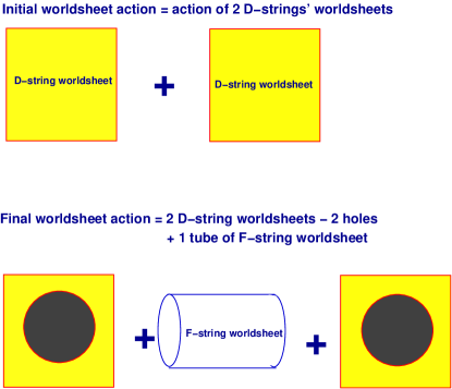
Figure 8: For D-strings to annihilate, F-strings must connect the D and anti-D strings.

The probability to go from a D-string worldsheet + anti-D-string worldsheet to 2 punctured worldsheets + a tube of fundamental string worldsheet can be thought of as the conditional probability $P({\rm annihilation}|D1,\bar{D}1)$. Using the definition of a conditional probability and probability in quantum theory

$$P({\rm annihilation}|D1,\bar{D}1)=\frac{P({\rm annihilation})}{P(D1,\bar{D}1)}\approx\frac{|e^{-S_{2}}\sqrt{\det{S_{2}^{\prime\prime}}}^{-1}|^{2}}{|e^{-S_{1}}\sqrt{\det{S_{1}^{\prime\prime}}}^{-1}|^{2}}=Ae^{-2B}$$ (70)

where $B=S_{2}-S_{1}$ and $A$ is the determinant prefactor providing the first quantum corrections. Then difference in action $B$, of the two configurations is the loss due to the 2 holes of the D1,${\rm\bar{D}}$1 worldsheets which are cut out and the addition of a tube of fundamental string worldsheet

$$B=\mu_{F}\cdot L\cdot 2\pi R-2\mu_{D1}\cdot\pi R^{2}$$ (71)

where $R$ is the radius of the hole and $L$ is the length of the tube. $R$ is chosen to minimize the tunneling action $B$.

$$\frac{\partial B}{\partial R}=0\;\;\;\Rightarrow\;\;\;R_{min}=\frac{L}{2}\frac{\mu_{F}}{\mu_{D1}}\;\;\;\Rightarrow B(R_{min})=\frac{\pi L^{2}\mu_{F}}{2}\left(\frac{\mu_{F}}{\mu_{D1}}\right)$$ (72)

Because the D-strings sit at the severely redshifted bottoms of resolved conifold throats, $\mu_{D1}=\frac{1}{2\pi\alpha^{\prime}g_{s}}e^{2A}$. However, because the F-strings connecting the $D1$s and $\bar{D}1$s pass through the bulk and much of their length is in the bulk their tensions are not redshifted. Hence $\mu_{F}=\frac{1}{2\pi\alpha^{\prime}}$ and $\mu_{D1}=\mu_{F}g_{s}^{-1}e^{2A}\sim\mu_{F}g_{s}^{-1}\cdot 10^{-8}$. If $L\sim 1$ in string units then [23]

$$P({\rm annihilation}|D1,\bar{D}1)=Ae^{-g_{s}\cdot 10^{8}}\ll 1$$ (73)

Hence, even if the $D1$ and its mirror ${\bar{D}}1$ are separated by only a few string lengths but are at the bottoms of mirror throats, the probability of annihilation is extraordinarily small. Likewise, it is very improbable for fundamental strings to emerge from one throat and interact with fundamental strings in the mirror throat. Thus strings and/or D-strings at the bottom of a heavily warped throat are largely decoupled from what happens in another throat or the unwarped part of the compactification manifold.

Long strings can also disappear by the pair production of the 4D baryons introduced in $\S\ref{sectionbaryon}$. This is analogous to how cosmic strings can break apart by pair production of monopoles and anti-monopoles. If a 3-cycle $A$ has $M$ units of flux through it as in (52) and is wrapped by $D3$ branes, then a $(p,q)$ string can break on $A$ into a $(p,q)$ string “entering” the baryon, and a $(p-M,q)$ string leaving the baryon. See figure 9.

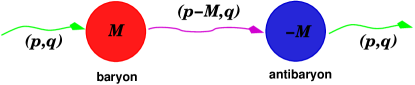
Figure 9: Baryon-antibaryon nucleation. If a $(p,q)$ string ends on $M$, then a $(p-M,q)$ string must connect the baryon and antibaryon.

A baryon and an antibaryon will be connected by a $(p-M,q)$ open string as shown in figure 9. The endpoint of a string which ends on the baryon will trace out the boundary of a string’s 2D worldsheet. Because the string worldsheet is invariant under Lorentz transformations along its surface, the string endpoint will trace out a curve (i.e. for a point particle theory this would be the hyperboloid $x^{2}+y^{2}+z^{2}-t^{2}=R^{2}$).

$$\sigma^{2}-\tau^{2}=R^{2}$$ (74)

where $R$ is some constant. Wick rotation, $\tau\rightarrow-i\tau$ turns the non-compact string worldsheet into a circle, since

$$\sigma^{2}+\tau^{2}=R^{2}$$ (75)

Thus the baryon and antibaryon will move along a circle just as in the well known Schwinger pair production process. The force on a baryon being tugged by two strings is $F=\mu_{(p,q)}-\mu_{(p-M,q)}$. The baryon action is then

$$S_{B}=-m\int ds-\int Vds$$ (76)

where $V$ is the potential energy. After a Wick rotation, $S_{B}$ picks up a minus sign,

$$S_{B}^{E} = m\int ds+\int Vds$$ (77)

$$= m\int ds+\int\partial V\cdot dA$$

$$= m\int ds-(\mu_{(p,q)}-\mu_{(p-M,q)})\int dA$$

$$= m\cdot 2\pi R-(\mu_{(p,q)}-\mu_{(p-M,q)})\cdot\pi R^{2}$$

In the last line we have used the Euclidean baryon trajectory (75). $m$ is the baryon mass which is the mass of the $D3$ brane wrapped on the $S^{3}$ [89]

$$m=\mu_{D3}\textsf{Vol}(S^{3})=\beta\frac{M^{3/2}}{2\pi\alpha^{\prime 2}g_{s}}$$ (78)

where Vol$(S^{3})$ is a constant $\beta$ times $M^{3/2}$. Minimizing (77) with respect to $R$ gives,

$$R=\frac{m}{(\mu_{(p,q)}-\mu_{(p-M,q)})}$$ (79)

Thus [23]

$$S_{B}^{E} = \frac{\pi m^{2}}{\mu_{(p,q)}-\mu_{(p-M,q)}}$$ (80)

$$= \frac{\pi[\mu_{D3}\cdot\textsf{Vol}(S^{3})]^{2}}{\mu_{F}(\sqrt{p^{2}+q^{2}/g_{s}^{2}}-\sqrt{(p-M)^{2}+q^{2}/g_{s}^{2}})}$$

$$\sim \frac{qM^{2}}{2p-M}$$

where in (80) we obtained the last line by taking the $g_{s}\ll 1$ limit. As $S_{B}^{E}$ can be very small for large $p$, $(p,q)$ strings can break apart on baryons. However, if $|p|<M/2$ then $S_{B}^{E}$ becomes negative. Since $S_{B}^{E}=S_{2}-S_{1}$ which is the action of the final state with a $(p-M,q)$ string and baryon pair production minus the action of just a $(p,q)$ string, if $|p|<M/2$, the initial state has larger action than the final state. Hence baryon pair production does not occur for small $p$ as argued in (24).

Now $M$ is constrained by (57) so that $M\mathrel{\hbox to0.0pt{\lower 4.0pt\hbox{\hskip 1.0pt$\sim$}\hss}\raise 1.0pt\hbox{$>$}}12$. Thus low $p$ and $q$ strings will be stable. $\S$7.2 discusses how a $(p,q)$ string network ends up being composed of the lightest strings which are $(\pm 1,\pm 1)$ and $(\pm 1,0)$ and $(0,\pm 1)$ strings. Breakage on baryons aids this migration towards lowest mass strings.

6 String reconnection probability

The probability that two colliding field theory strings reconnect is essentially one [54] (although see [90]). However, the same probability for superstrings is suppressed by a factor of $g_{s}^{2}$ and can thus be much less than one. Thus a reconnection probability $P<1$ is one of the distinguishing features of superstrings. Below we give a simplified account of the reconnection probabilities calculated in [41].

The following is a rather interesting application of tree-level string scattering. The most important string theory factors which show up in $P$ are $g_{s}^{2}$ and a velocity function. The $g_{s}^{2}$ factor is the reason why superstrings intercommute much more infrequently than field theory strings. The velocity function for the F-string goes to infinity for small and large $v$ hinting that $F$ strings tend to intercommute at extreme $v$. For the D-strings, the velocity function blows up at high $v$ and reconnection is also very probable for $v\sim 0$. Another very important factor in $P$ is a geometrical factor measuring how often “strings miss each other” when moving in the extra dimensions.

6.1 Reconnection of F-strings

Two strings which collide will exchange gravitons and massless particles. In the $t$ channel and forward scattering small $t$ limit we expect the tree level scattering amplitude to have a pole at $t=0$. Because we are calculating graviton exchange, the amplitude should be weighted by Newton’s constant $G_{d}\sim\kappa^{2}\sim g_{s}^{2}$. We should also have a factor of $V$ in the denominator if we box normalize the string wavefunctions. If for convenience we put the strings on a large 2-torus and a 6D small compact manifold with volume $V_{\perp}$, then $V=V_{\perp}V_{T^{2}}$. Now in the large energy $s\gg 0$ (and fixed $t$) limit, string amplitudes display Regge behavior – i.e. ${\cal{A}}\sim s^{\alpha_{0}(t)}$ where $\alpha_{0}(t)$ is a linear function of $t$. In this case $\alpha_{0}(t)=1+\frac{\alpha^{\prime}t}{4}$. When we analytically continue from Euclidean to Lorentzian momentum the $s^{\alpha^{\prime}t/4}$ generates a multiplicative factor of $e^{-i\pi\alpha^{\prime}t/4}$. Thus in the small $t$ and large $s$ limit

$${\cal{A}}\sim-\frac{g_{s}^{2}}{V}\frac{s^{1+\frac{\alpha^{\prime}t}{4}}}{t}e^{-i\pi\alpha^{\prime}t/4}$$ (81)

We can calculate the total probability of intercommutation using the optical theorem

$$P = \frac{1}{4E_{1}E_{2}v}2\;{\rm Im}\;{\cal{A}}|_{t\rightarrow 0}$$ (82)

The imaginary part of ${\cal{A}}$ comes from $\textsf{Im}(e^{-i\pi\alpha^{\prime}t/4})=-\sin\pi\alpha^{\prime}t/4$, which combined with the $1/t$ pole factor gives the finite result $-\pi\alpha^{\prime}/4$ as $t\rightarrow 0$. Now because of the $V_{\perp}$ in $V$ in (81) we expect $P\sim 1/V_{\perp}$. We expect the volume of the torus $V_{T^{2}}$ to disappear. Otherwise our results will depend on the size of the large wrapped dimensions. In the $t\rightarrow 0$ limit, $s^{1+\frac{\alpha^{\prime}t}{4}}\rightarrow s$. The $E_{1}E_{2}$ in (82) will then cancel out the energy dependence coming from the $s$ in ${\cal{A}}|_{t\rightarrow 0}$. Hence, only geometrical factors depending on the angle $\theta$ and velocity $v$ will be left over. Thus we expect

$$P=g_{s}^{2}\frac{V_{min}}{V_{\perp}}f(\theta,v)$$ (83)

$V_{min}=(2\pi\sqrt{\alpha^{\prime}})^{6}$ is a constant factor which appears to make $P$ dimensionless, and represents the volume of a T-dual 6D torus – the minimum volume torus in string theory. $f(\theta,v)$ is an ${\cal{O}}(1)$ function of $\theta$ and $v$ as long as $v$ is not too relativistic or not too small. We would expect that static F-strings intersecting in a non-BPS way will reconnect and hence it is not surprising that blows up as $f\sim 1/v$ as small $v$. At high velocity $f$ also diverges. This is coming from the distinctive Regge effect of strings. Strings tend to interact more strongly at higher energies thus $P$ grows with increasing $v$.

The probability that a moving F-string breaks and connects with a $(p,q)$ string can be estimated in a similar way. The result is identical to (83) with $f(\theta,v)$ replaced by a different ${\cal{O}}(1)$ $p,q$ dependent function $h_{p,q}(\theta,v)$ which reduces to $f(\theta,v)$ for $p=1,q=0$ ($h_{1,0}=f)$.

$$h_{p,q}=\frac{1}{g_{s}^{2}v}\frac{q^{2}v^{2}+g_{s}(p-\cos\theta\sqrt{(1-v^{2})(p^{2}+q^{2}/g_{s}^{2})})}{8\sin\theta\sqrt{(1-v^{2})(p^{2}+q^{2}/g_{s}^{2})}}$$ (84)

6.2 Reconnection for strings with D-string charge

The intercommutation of D-strings is more complex. Reconnection/intercommutation is a tree-level process for F-F and $F-(p,q)$ interactions. The end-state of the tree-level supergravity solution of colliding F-strings, or F-strings colliding with a $(p,q)$ string is a reconnected string. However, D-D and $(p,q)-(p^{\prime},q^{\prime})$ string intercommutation is a 1-loop open string quantum process because open string (tachyons) must be nucleated to glue the D-strings together. The classical solution corresponds to D-strings passing through each other [91].

Because D-strings are composite objects in the sense that they may be surrounded by a halo of open strings, D-D and $(p,q)-(p^{\prime},q^{\prime})$ reconnection is also qualitatively different from F-F reconnection. For example, D-strings at high energy are surrounded by a halo of energetic open strings. When a D-string passes another D-string, strings in the halo of one D-string may connect with strings in the halo of the onrushing D-string, or equivalently open strings may be nucleated between the two branes. These open strings can then pull the D-strings toward one another and eventually cause reconnection. The energy to pair produce the open strings is interestingly recaptured from the work done to stretch the nucleated strings by the moving D-strings. Thus the faster the strings move past each other the heavier the nucleated strings may be and the longer they may be [92, 93]. This unusual feature simply reflects the Regge nature of string scattering – that like fundamental strings, their scattering cross-section grows with velocity. In 6 compact directions, for $v\mathrel{\hbox to0.0pt{\lower 4.0pt\hbox{\hskip 1.0pt$\sim$}\hss}\raise 1.0pt\hbox{$<$}}1$, the D-strings act as 6D black disks of area $\sigma\sim\alpha^{\prime 3}(-\ln(1-v^{2}))^{3}$ [41, 92]. However, as the average $v^{2}$ for a cosmic string is $<\frac{1}{2}$, we will concentrate on much smaller velocities. Note however, that as two branes approach each other light closed strings are radiated by the branes and this gives rise to an inter-brane potential of $V\sim-v^{4}$ [94, 95]. However, open strings are needed to glue the two branes together for reconnection.

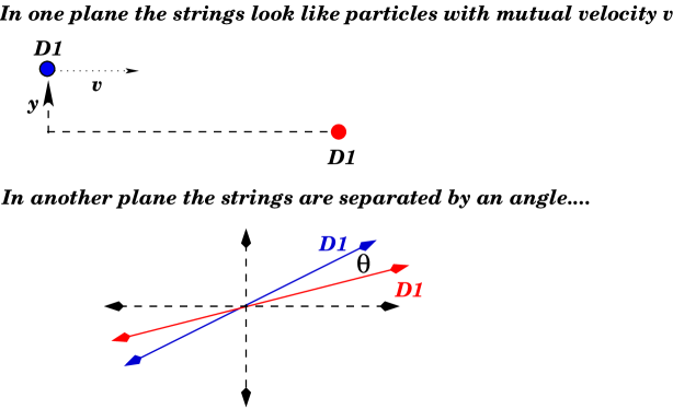
Figure 10: $y$ is the impact parameter and $\theta$ the angle between 2 D-strings in a particular 2D plane.

For $v\ll 1$ only the lowest mass string state will contribute to the string scattering/reconnection amplitude. If the branes are tilted by an angle $\theta$ in the transverse directions, then for generic values of $\theta$ the lowest mass state is a tachyon with mass $m^{2}=\frac{y^{2}}{(2\pi\alpha^{\prime})^{2}}-\frac{\theta}{2\pi\alpha^{\prime}}$. Here, $y$ is the impact parameter. See figure 10. A tachyon will appear once $y<\sqrt{2\pi\alpha^{\prime}\theta}$. Once the tachyon appears the branes are almost sure to reconnect for small $v$. (Note, there is an interplay between $\theta$ and $y$. As $\theta$ decreases, it becomes harder to excite tachyons if $y\neq 0$ because the branes become more parallel and parallel branes are not tachyonic.) For $y\leq\sqrt{2\pi\alpha^{\prime}\theta}$, reconnection occurs and the low $v$ cross-section for tachyon pair production/reconnection is the black sphere cross section, $\sigma=\textsf{Ball}_{6}=\frac{\pi^{3}}{6}y^{6}=\frac{1}{6}(2\pi^{2}\alpha^{\prime}\theta)^{3}$. Thus, the probability of tachyon pair production $P_{pp}$ which in this case is the same as the reconnection probability $P$ for $v\rightarrow 0$ is (if we ignore the factor of $\frac{1}{6}$ as JJP do)

$$P_{pp}=P(v\rightarrow 0)=\frac{(2\pi^{2}\alpha^{\prime}\theta)^{3}}{V_{\perp}}=\frac{V_{min}}{V_{\perp}}\left(\frac{\theta}{2}\right)^{3}$$ (85)

This is very similar to (83). In the small $\theta$ and small $v$ limit, $f(\theta,v)=h_{1,0}(\theta,v)=\frac{\theta^{3}}{8v}$. Thus apart from a factor of $\frac{1}{v}$, the F-F reconnection probability is the same as the tachyon pair production probability for D-D reconnection.

For $v^{2}\sim\frac{1}{2}$, higher mass states, in particular states whose mass vanishes with vanishing $\theta$ will contribute to the open string pair production probability $P_{pp}$. Using the standard formalism of Schwinger pair production in [96], $P_{pp}$ can be related to the scattering amplitude ${\cal{A}}(y)$ as

$$1-P_{pp}(y) = |\;e^{i{\cal{A}}(y)}|^{2}=\;e^{-2\,{\rm Im}\,{\cal{A}}(y)}={\prod_{i,{\rm fermions}}(1-x_{i})}{{\prod_{j,{\rm bosons}}\frac{1}{(1+x_{j})}}}$$ (86)

where $x_{k}=e^{-2\pi\alpha^{\prime}m^{2}_{k}/\epsilon}$. Here $m_{k}$ is the mass of the string state $k$ and the velocity is $v=\tanh\pi\epsilon$ where $\pi\epsilon$ is the rapidity.

We can understand (86) as follows. The first two equations on the L.H.S of (86) follow from Schwinger’s prescription. The R.H.S results from evaluating ${\cal{A}}$ which is essentially the 1-loop vacuum energy of two branes with relative velocity $v$. The 1-loop vacuum amplitude can be calculated using the Coleman-Weinberg formula: ${\cal{A}}=E_{vac}\sim\int\frac{dt}{t}Z(t)\sim\int\frac{dt}{t}\sum_{i}e^{-tm_{i}^{2}/2}$ [45, 97]. Now the sum over $i$ is over all bosonic and fermionic open string states connecting the two branes. The sum can be written in terms of Jacobi $\vartheta_{a}$ functions; in particular $Z(t)\propto 1/\vartheta_{1}(\epsilon t|it)$. This has poles at the zeros of $\vartheta_{1}(\epsilon t|it)$ which are at $\epsilon t=1,2,3,...$. Because of these poles, ${\cal{A}}$ has an imaginary part which is the sum of the residues of the poles of the partition function: $\sum_{n=1}^{\infty}\textsf{ Res}[Z(\frac{n}{\epsilon})]$.

We now define the fermionic partition function $Z_{f}(t)=\sum_{i}e^{-2\pi\alpha^{\prime}tm_{i}^{2}}$ which sums over all fermionic open string states $i$ and define the bosonic partition function $Z_{b}(t)=\sum_{j}e^{-2\pi\alpha^{\prime}tm_{j}^{2}}$, which sums over all bosonic open string states $j$. Perhaps unsurprisingly the sum over residues $\sum_{n=1}^{\infty}\textsf{Res}[Z(\frac{n}{\epsilon})]$ can be related to individual partition functions $Z_{b}$ and $Z_{f}$ as

$$-2{\rm Im}{\cal{A}}(y) = -\sum_{n=1}^{\infty}\left[\frac{(-)^{n+1}}{n}Z_{b}\left(\frac{n}{\epsilon}\right)+\frac{1}{n}Z_{f}\left(\frac{n}{\epsilon}\right)\right]$$ (88)

$$= \sum_{j}\left(\sum_{n=1}^{\infty}(-)^{n}\frac{x_{j}^{n}}{n}\right)-\sum_{i}\left(\sum_{n=1}^{\infty}(-)^{n}\frac{(-x_{i})^{n}}{n}\right)$$

$$= \ln\prod_{i}\frac{1}{1+x_{i}}+\ln\prod_{j}(1-x_{j})$$

finally yielding the R.H.S of (86).

The bosonic states whose mass vanishes as $\theta,y\rightarrow 0$ have $m^{2}_{j}=\frac{y^{2}}{(2\pi\alpha^{\prime})^{2}}-\frac{(3-2j)\theta}{2\pi\alpha^{\prime}}$ with multiplicities of state $\{j\}=\{1,2,3...\}$ being $\{1,7,8,8,8,8,...,8,...\}$. The analogous fermionic states $\{i\}=\{1,2,3...\}$ have $m_{i}^{2}=\frac{y^{2}}{(2\pi\alpha^{\prime})^{2}}-\frac{(2-2i)\theta}{2\pi\alpha^{\prime}}$ with multiplicities $\{4,8,8,8,8,...,8,...\}$. For, $v^{2}\sim\frac{1}{2}$, the rapidity parameter is $\epsilon\approx 0.3$. For an angle $\theta$ of order 1, we then find $e^{-\theta/\epsilon}\simeq 0.04$. Thus ignoring the $y$ dependence we have $x_{j}=e^{-2\pi\alpha^{\prime}m^{2}_{j}/\epsilon}\propto e^{-2j\theta/\epsilon}$ and $x_{i}=e^{-2\pi\alpha^{\prime}m^{2}_{i}/\epsilon}\propto e^{-2i\theta/\epsilon}$ and $x_{i}$ and $x_{j}$ decrease exponentially with increasing $i$ and $j$ respectively. (Note, here $i$ is not the imaginary unit $\sqrt{-1}$.) Thus we can ignore states with high $i$ or $j$ in (86). If fact if we restrict to $j=1$ which corresponds to the bosonic tachyon, and $i=1$ which corresponds to the lightest fermion, then (86) is

$$1-P_{pp}\simeq\frac{(1-e^{-{y^{2}/2\pi\alpha^{\prime}\epsilon}})^{4}}{1+e^{-{y^{2}/2\pi\alpha^{\prime}\epsilon}+{\theta/\epsilon}}}$$ (89)

The open string pair production probability $P_{pp}$ rapidly decays to 0 as $y$ increases. See figure 12. However, if the strings do collide then $y=0$ at the moment of collision and $P_{pp}\simeq 1$. This implies that open string pairs are always produced for $y=0$. These open string pairs will always lead to reconnection unless $g_{s}\ll 1$. For $\theta$ small, more open string states must be included in (89). However, JJP claim that $P_{pp}\simeq 1$ in most cases.

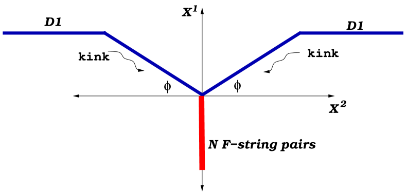
Figure 11: A moving D-string nucleates $N$ F-string pairs. Two kinks are created which move with velocity 1 in the $X^{2}$ and $-X^{2}$ directions. The D-string moves upward with velocity $u$. The strings are shown in the rest frame and for a stable intersection the string intersection angle is $\phi$.

For $g_{s}\ll 1$ the colliding strings are very massive since $\mu_{(p,q)}\sim\mu_{F}\frac{1}{g_{s}}$. Thus one might expect that the colliding strings will pass through each other unless ${\cal{O}}(\frac{1}{g_{s}})$ open strings are nucleated gluing the D-strings together. JJP argue that at least

$$N>\frac{1}{g_{s}}\sinh\frac{\pi\epsilon}{2}$$ (90)

open string pairs must be produced for intercommutation to occur. This essentially comes from doing a force balance calculation as in $\S\ref{sectionpq}$ at some time $t$ as in figure 11. Figure 11 shows a string vertex at the origin of the $(X^{2},X^{1})$ plane with $2N$ F-strings lying along the negative $X^{1}$ axis attached to a D-string which is shown in blue in figure 11. The kinked parts of the D-string make an angle $\phi$ with the $X^{2}$ axis. Force balance determines $\phi$ to be $2\mu_{D1}\sin\phi=2N\mu_{F}$. When the two D-strings scatter two kinks are created on each D-string which move in opposite directions along the strings at the speed of light. The speed at which D-strings are moving past each other in the $X^{1}$ direction is the center of mass speed $u=\tanh\frac{\pi\epsilon}{2}$. JJP argue that if $u>\tanh\frac{\pi\epsilon}{2}$ reconnection will not occur because of the following.

Go to the rest frame to avoid worrying about the angle $\phi$ being boosted. Then each kink will be moving horizontally in the $+X^{2}$ or $-X^{2}$ direction with velocity 1 (since relativistic cosmic string kinks move at the speed of light) and will be moving upwards in the $X^{1}$ direction with velocity $u$ and thus will effectively be moving at an angle $\arctan u$. The vertex will be stable if $\arctan u=\phi$. However, if the D-strings are moving very fast past each other then $\arctan u>\phi$ and the vertex will be unstable and the strings will pass by/through each other. Thus the nucleated $F$ strings will glue the moving D-strings together and cause D-string reconnection only if $u<\tan\phi$. This condition then gives (90).

JJP argue that the open string pairs are produced in a squeezed state and that these strings will be the lightest possible strings – tachyons [98, 99, 100, 101]. If $p$ is the probability of pair producing a pair of strings in a squeezed state of one oscillator, then $p^{N}$ is the probability of producing $N$ pairs. For a tachyon $p\simeq(1-e^{-\theta/\epsilon})$, thus $p^{N}\simeq\exp(-Ne^{-\theta/\epsilon})$. Using the value of $N$ in (90) the probability of D-D reconnection is

$$P(y=0)\simeq\exp\left({-\frac{1}{g_{s}}\sinh\frac{\pi\epsilon}{2}e^{-\theta/\epsilon}}\right)$$ (91)

which interestingly is a non-perturbative result because of the $1/g_{s}$ and was qualitatively verified by [91] using an effective theory approach. (Note, in addition to tachyons, 4 fermionic pairs are also produced with essentially unit probability. JJP’s version of (91) is the probability of producing $N-4$ tachyons and 4 fermions. We have focused only on the tachyons because as soon as $y\neq 0$ fermion production is suppressed relative to tachyon production.)

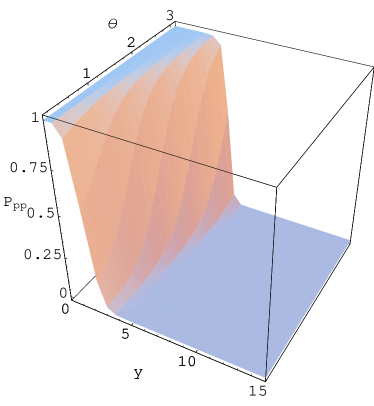
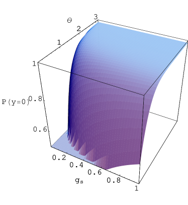
Figure 12: (1) The left figure shows that the pair production probability $P_{pp}$, falls rapidly with $y$. (2) The figure on the right shows that the probability that colliding D-strings will reconnect $P(y=0)$ is $\simeq 1$ for $\theta\sim 1$ and $g_{s}\mathrel{\hbox to0.0pt{\lower 4.0pt\hbox{\hskip 1.0pt$\sim$}\hss}\raise 1.0pt\hbox{$>$}}0.2$. For small values of $g_{s}$ and/or $\theta$, $P(y=0)\ll 1$. Both calculations only take the 2 lightest string modes into account.

For $g_{s}\rightarrow 0$ but $v\neq 0$, the reconnection probability vanishes, $P\rightarrow 0$. But it doesn’t start to nosedive until $g_{s}$ becomes small. For example, if $g_{s}\sim 0.1$ and $\theta\sim 1,\epsilon=0.3$ we find $P=0.7$. For smaller angles $\theta<1$, higher mode states must be taken into account in (91) and $P$ can decrease significantly, see figure 12. Thus, although $P\simeq 1$ generally, there is a range of small angles where there is a significant probability of D-strings passing through each other.

Equation (91) gives the probability that colliding D-strings will reconnect. The probability that a random D-string will collide with another random D-string and reconnect is: the probability that the two strings will run into each other: $\sigma(v)/V_{\perp}^{DD}$ where $\sigma(v)$ is the scattering cross-section, times (91) extended to finite $y$. However, $P(y)\sim 0$ if $y$ is much larger than a few string lengths. Also, for $v$ not extremely relativistic, $\sigma(v)$ doesn’t grow much larger than the black sphere $\sigma(0)$ in (85) since $\sigma(v)$ grows logarithmically with $v$ [41, 92]. Thus we can approximate the reconnection probability for random D-strings to be the probability that two strings come within $\sqrt[6]{\sigma(0)}\sim\sqrt{2\pi\alpha^{\prime}\theta}$ of each other such that tachyons are excited, times the probability that enough open strings are pair produced to induce reconnection. Thus

$$P\sim\frac{V_{min}}{V_{\perp}}\left(\frac{\theta}{2}\right)^{3}\exp\left({-\frac{1}{g_{s}}\sinh\frac{\pi\epsilon}{2}e^{\frac{y^{2}}{2\pi\alpha^{\prime}\epsilon}-\frac{\theta}{\epsilon}}}\right)\simeq\frac{V_{min}}{V_{\perp}}\left(\frac{\theta}{2}\right)^{3}\Theta\biggl{(}\sqrt{2\pi\theta\alpha^{\prime}}-y\biggr{)}$$ (92)

The exponential factor in (92) is $\simeq 1$ for $y<\sqrt{2\pi\theta}$ and vanishes for $y\mathrel{\hbox to0.0pt{\lower 4.0pt\hbox{\hskip 1.0pt$\sim$}\hss}\raise 1.0pt\hbox{$>$}}\sqrt{2\pi\theta\alpha^{\prime}}$. Thus we replaced the exponential factor by the Heaviside function on the R.H.S. which is zero if $y$ is too large to excite any tachyons. Note the exponential inside the exponential is simply $\exp[-(\textrm{tachyon mass})^{2}/(2\pi\alpha^{\prime}\epsilon)]$. The fermions don’t contribute much to (92) because their pair production probability $p$ vanishes much faster than $p$ for tachyons once $y\mathrel{\hbox to0.0pt{\lower 4.0pt\hbox{\hskip 1.0pt$\sim$}\hss}\raise 1.0pt\hbox{$>$}}\sqrt{2\pi\theta\alpha^{\prime}}$.

For $(p,q)$ and $(p^{\prime},q^{\prime})$ strings, the nucleated open strings have $q$ ways of connecting to the $(p,q)$ string and $q^{\prime}$ ways of connecting to the $(p^{\prime},q^{\prime})$ string. Thus the multiplicities of the $i$ and $j$ states will change by a multiplicative factor of $|qq^{\prime}|$. Also since adding F-string flux to a string may be thought of as boosting the string, the rapidity $\epsilon$ and angle $\theta$ will change to some new $\tilde{\epsilon}$ and $\tilde{\theta}$. The formulae are given on page 22 of [41]. But after substituting the new $\tilde{\epsilon}$ and $\tilde{\theta}$ and increasing the degeneracy we find for just tachyon pair production at $y=0$

$$(1-P_{pp})=\frac{1}{(1+e^{\tilde{\theta}/\tilde{\epsilon}})^{|qq^{\prime}|}}\simeq e^{-|qq^{\prime}|\tilde{\theta}/\tilde{\epsilon}}$$ (93)

and thus $p$ in the paragraph above (91) becomes $p\simeq 1-e^{-|qq^{\prime}|\tilde{\theta}/\tilde{\epsilon}}$, and $\frac{1}{g_{s}}e^{-\tilde{\theta}/\tilde{\epsilon}}$ in (91) will be replaced by $\frac{1}{g_{s}}e^{-|qq^{\prime}|\tilde{\theta}/\tilde{\epsilon}}$. Hence a small $g_{s}$ can be compensated by a large $q$ or $q^{\prime}$, allowing $P\simeq 1$ for a much larger range of $g_{s}$. However, if $y\neq 0$, then $e^{\frac{y^{2}}{2\pi\alpha^{\prime}\epsilon}-\frac{\theta}{\epsilon}}$ in (92) is replaced by $e^{|qq^{\prime}|(\frac{y^{2}}{2\pi\alpha^{\prime}\tilde{\epsilon}}-\frac{\tilde{\theta}}{\tilde{\epsilon}})}$ allowing the middle expression of (92) to possibly decay to zero even faster for suitable values of $\tilde{\epsilon},\tilde{\theta}$ once $y\mathrel{\hbox to0.0pt{\lower 4.0pt\hbox{\hskip 1.0pt$\sim$}\hss}\raise 1.0pt\hbox{$>$}}\sqrt{2\pi\tilde{\theta}\alpha^{\prime}}$.

6.3 What is $V_{\perp}$ if the strings’ position moduli are fixed?

Cosmologists tend to regard the spatial positions of objects like cosmic strings, domain walls, and monopoles as free. They are free to move, collide and do whatever external forces push them to do. However, in string theory the positions of strings, branes, etc., are scalar fields. They are unprotected by any symmetry. Hence, there is nothing to prevent their positions from being fixed and prevent the generation of a potential fixing their positions. In fact, it is almost a mantra of faith among string theorists that unprotected fields must surely become fixed; else string theory would predict too many massless fields and violate the equivalence principle, etc.

In this section we will assume that the positions of cosmic strings are somehow fixed. If the positions are not fixed then $P$ can be hugely suppressed if the radius of the extra dimensions is say 100 string lengths or more ($R\sim 100\ell_{s}$), since then $V_{min}/V_{\perp}\sim(\ell_{s}/R)^{6}\sim 10^{-12}$.

Classically, there are several reasons to believe that strings will be localized in the extra dimensions. (1) Warped geometries naturally generate a potential by localizing objects at the bottom of a throat. I.e. it is very difficult to emerge from a heavily warped throat because of extreme redshifting. (2) Supersymmetry breaking generically generates potentials. (3) Tachyon condensation in the classical limit $g_{s}\rightarrow 0$ posits that all decay products like F, D and $(p,q)$ strings lie along the plane of the original hypersurface on which the condensation took place. This means such strings’ extra dimensional positions are fixed to lie on the hyperplane.

Note, we will assume the dilaton is constant throughout and hence that $\mu_{(p,q)}^{2}(Y)=\frac{1}{2\pi\alpha^{\prime}}(p^{2}+q^{2}e^{-2\phi(Y)})$ is a constant. JJP write $\mu_{(p,q)}(Y)=\frac{1}{2\pi\alpha^{\prime}}\nu(Y)$ to allow for a varying dilaton. Thus, wherever one sees $\nu(0)$ one should replace it by

$$\nu(0)\rightarrow 2\pi\alpha^{\prime}\mu_{(p,q)}$$ (94)

Let $Y^{i}$ be the coordinates of a string in the extra dimensions. We will assume that the potential $V(Y)$ fixing the strings’ positions comes from the warped metric. If the string is fixed at $Y^{i}=0$ we would like to calculate the quantum spread in position $\langle Y^{i}Y^{i}\rangle$. For a scalar $\phi$ in 2D with action $S=-\frac{Z}{2}\int d^{2}\sigma[(\partial_{a}\phi)^{2}+m^{2}\phi^{2}]$ as JJP mention a Feynman diagram calculation for the spread $\langle\phi^{2}\rangle$ yields

$$\langle\phi(0)\phi(0)\rangle=\frac{1}{Z}\int_{0}^{\Lambda}\frac{d^{2}k}{(2\pi)^{2}}\frac{1}{k^{2}+m^{2}}=\frac{1}{4\pi Z}\ln\frac{\Lambda^{2}+m^{2}}{m^{2}}$$ (95)

The UV cutoff is the string scale, $\Lambda^{2}\sim 1/\alpha^{\prime}$. But a 4D observer at the bottom of a warped throat will instead see the warped cutoff $\Lambda^{2}\sim m_{s}^{2}e^{2A(0)}=1/(\alpha^{\prime}e^{-2A(0)})$.

In flat space the worldsheet action for the position fields $Y^{i}$ contains a kinetic piece $\frac{\mu_{(p,q)}}{2}\int d^{2}\sigma(\partial_{a}Y^{i})^{2}$ and a potential piece $\int d^{2}\sigma V(Y)$ which we calculate later. Expanding the potential about the minimum $Y^{i}=0$ and assuming $V(0)=0$, we have $S\approx-\mu_{(p,q)}\int d^{2}\sigma\frac{1}{2}(\partial_{a}Y^{i})^{2}-\int d^{2}\sigma\frac{1}{2}V_{,ij}(0)Y^{i}Y^{j}$. Therefore, $k$ in (95) maps to $Z=\mu_{(p,q)}$ and $m^{2}$ in (95) maps to $m^{2}=\frac{2\pi\alpha^{\prime}V_{,ii}(0)}{\mu_{(p,q)}}$ where we have diagonalized the $V_{,ij}$ matrix by rotating the coordinates $Y^{i}$ among themselves. Then the analog of (95) is

$$\langle Y^{i}Y^{i}\rangle=\frac{\omega_{i}}{4\pi\mu_{(p,q)}};\ \ \ \ \ \ \ \omega_{i}=\ln\left(1+\frac{e^{2A(0)}\mu_{(p,q)}}{\alpha^{\prime}V_{,ii}}\right)$$ (96)

The localizing effects of warped geometries can be described by a potential as follows. The Nambu-Goto action for a string in the warped metric (37) is $-\mu_{(p,q)}\int d^{2}\sigma\sqrt{-h_{ab}}$ where $h_{ab}=e^{2A(y)}g_{\mu\nu}\partial_{a}X^{\mu}\partial_{b}X^{\mu}+e^{-2A(y)}\tilde{g}_{mn}\partial_{a}Y^{i}\partial_{b}Y^{j}$. Choosing $g_{\mu\nu}=\eta_{\mu\nu}$ and $X^{0}=\sigma^{0}$ and $X^{1}=\sigma^{1}$ the Nambu-Goto action becomes $\int d^{2}\sigma V(Y)$ where $V(Y)$ is the potential

$$V(Y)=-{\cal{L}}=\mu_{(p,q)}e^{2A(Y)}=\mu_{(p,q)}e^{2A(0)}\left(1-\frac{r^{2}}{R_{3}^{2}}\right)^{-1/2}$$ (97)

On the R.H.S. we specialized to the special case of flux compactifications discussed in $\S\ref{sectionfluxcompact}$. $R_{3}\approx\sqrt{g_{s}M\alpha^{\prime}}$ is the radius of the $S^{3}$ being blown up and $r$ is the parameter parameterizing how ‘long’ the throat is. The blown up $S^{3}$ is at $r=0$. Recall that $e^{2A(0)}\sim 10^{-8}$ from (56). Note, $V^{\prime\prime}(0)=V(0)/R_{3}^{2}$. This means that the spread of a string’s position in the directions along the throat and transverse to the $S^{3}$ will be $\langle Y^{i}Y^{i}\rangle=\frac{1}{4\pi\mu_{(p,q)}}\ln(1+g_{s}M)$ and $\omega_{i}=\ln(1+g_{s}M)$

Also note that $V(0)$ is constant on the $S^{3}$ ($r=0$). Hence $V$ doesn’t localize the strings on the $S^{3}$ and the strings are free to move all over the $S^{3}$. The occurs because of an $SU(2)\times SU(2)$ symmetry of the deformed conifold geometry (i.e of the throat geometry). However, once the throat is connected to a larger Calabi-Yau, this symmetry is expected to be broken because the overall CY lacks this $SU(2)\times SU(2)$ symmetry. This breaking presumably generates a potential on the $S^{3}$. The dimensionless throat length is approximately $e^{-A(0)}$. The further away the CY is the smaller its effect on the $S^{3}$. Thus its influence can be measured by the distance $e^{-A(0)}$ which translates to a mass scale $\alpha^{\prime}m^{2}\sim e^{2A(0)}$. Thus instead of being able to roam around the entire $S^{3}$, a string will we able to spread over a (distance)² of $\langle Y^{i}Y^{i}\rangle=\frac{1}{4\pi\mu_{(p,q)}}\ln(1+\frac{\Lambda^{2}}{m^{2}})=\frac{1}{4\pi\mu_{(p,q)}}\ln(1+e^{-2A(0)})$ since the redshift factors $e^{2A(0)}$ of $\Lambda^{2}$ and $m^{2}$ cancel. Since $e^{2A(0)}\sim 10^{-8}$, $\langle Y^{i}Y^{i}\rangle\sim\frac{1}{4\pi\mu_{(p,q)}}\ln e^{-2A(0)}$ and $\omega_{i}\sim\ln e^{-2A(0)}=-2A(0)$.

Thus we can estimate $V_{\perp}\sim(\langle Y^{i}Y^{i}\rangle)^{3}$. This increases logarithmically with the mass of the $Y^{i}$ fields, $V_{,ii}$. This method gives the correct dependence on the various parameters but may miss out some numerical factors. A more clever way to estimate the volume is to use a delta function $\delta^{6}(Y)$ as an inverse volume operator since $\delta(x)=\frac{1}{V}$ and evaluate $\langle\delta^{6}(Y)\rangle$. Note the $V_{\perp}$ appearing in the reconnection probability will depend on the kinds of string being scattered and we will label it accordingly.

Suppose F and D strings are localized in the same area. Fluctuations in F-string positions will be much larger than D-string position fluctuations unless, $g_{s}\simeq 1$. Thus we can approximate the D-strings as fixed and find the F-string fluctuation about a fixed center – the D-strings’ position, $Y^{i}=0$. This means we take $\mu_{(p,q)}$ in (96) to be $\mu_{F}$.

$$\frac{V_{min}}{V_{\perp}^{FD}}=V_{min}\langle\delta^{6}(Y)\rangle=V_{min}\int\frac{d^{6}k}{(2\pi)^{6}}\langle e^{ik\cdot Y}\rangle=\int\frac{d^{6}k}{\alpha^{\prime-3}}e^{-k_{i}k_{j}\langle Y_{i}^{2}\rangle/2}=\prod_{i=1}^{6}\sqrt{\frac{4\pi}{\omega_{i}}}$$ (98)

The expectation value $\langle e^{ik\cdot Y}\rangle$ was calculated using a Gaussian wavefunction since to 2$nd$ order the strings are confined by a harmonic oscillator potential, $V=V_{,ij}Y^{i}Y^{j}$. Thus $\langle e^{ik\cdot Y}\rangle$ is just the Fourier Transform of the normal distribution and ${\cal{F}}(\frac{e^{-x^{2}/2a^{2}}}{\sqrt{2\pi a^{2}}})=e^{-a^{2}k^{2}/2}$.

If the $SU(2)\times SU(2)$ of the $S^{3}$ is unbroken such that strings can freely wander all over the $S^{3}$ then (98) breaks up into a part measuring the fluctuations over the $S^{3}$ $V_{min}(3D)/V_{\perp}(S^{3})$ times a part giving the fluctuations over the other 3 compact directions $\prod_{1}^{3}\sqrt{4\pi/\omega_{i}}$. Here, $V_{\perp}(S^{3})$ is the volume of the $S^{3}$ and $V_{min}(3D)=(2\pi\sqrt{\alpha^{\prime}})^{3}$ is the minimal (T-dual) 3D volume in string theory. The second factor arises because the strings are confined by the warped factor potential in the 3 compact directions transverse to the 3 directions of the $S^{3}$. Now $V_{\perp}(S^{3})=2\pi^{2}R_{3}^{3}=2\pi^{2}\ell_{s}^{3}(g_{s}M)^{3/2}$ and $\omega_{i}=\ln(1+g_{s}M)$ for $i$ in the non-$S^{3}$ compact directions. This gives the first expression of the R.H.S. of (99).

If an $SU(2)\times SU(2)$ breaking potential is generated, then as discussed above, $\omega_{i}$ in the $S^{3}$ directions is $\ln e^{-2A}$, or equivalently $\ln H^{1/2}(0)$ in JJP’s notation where $H^{1/2}(Y)=e^{-2A(Y)}$. Then (98) becomes the second expression of (99). For some choice of parameters as the fluctuations spread out over the $S^{3}$, the second expression (99) becomes smaller than the first expression. This is due to limitations of the calculation. We then choose the maximum of the two expressions.

$$\frac{V_{min}}{V_{\perp}^{FD}}=\max\left[\frac{4\pi}{(g_{s}M)^{3/2}}\frac{(4\pi)^{3/2}}{\ln^{3/2}(1+g_{s}M)}\ ,\ \frac{(4\pi)^{3}}{\ln^{3/2}(e^{2A(0)})\ln^{3/2}(1+g_{s}M)}\right]$$ (99)

Suppose the F strings are localized at a distance $(Y_{D}^{i}Y_{D}^{i})^{1/2}$ away from the D-strings. Then in for example the unbroken $SU(2)\times SU(2)$ case, $1/V_{\perp}^{FD}$ is not suppressed by $(Y_{D}^{i}Y_{D}^{i})^{-3/2}$. Rather it is exponentially suppressed as

$$\frac{V_{min}}{V_{\perp}^{FD}}|_{Y_{D}^{i}}=V_{min}\langle\delta^{6}(Y-Y_{D})\rangle=\prod_{i=1}^{6}\sqrt{\frac{4\pi}{\omega_{i}}}e^{-\sum_{1}^{6}\frac{Y_{D}^{i}Y_{D}^{i}}{\alpha^{\prime}\omega_{i}}}=\frac{V_{min}}{V_{\perp}^{FD}}e^{-\sum_{1}^{6}\frac{Y_{D}^{i}Y_{D}^{i}}{\alpha^{\prime}\omega_{i}}}$$ (100)

because the exponent $\langle Y^{i}Y^{j}\rangle$ in (98) is replaced by $\langle(Y^{i}-Y^{i}_{D})(Y^{j}-Y^{j}_{D})\rangle=\langle Y^{i}Y^{j}\rangle+Y_{D}^{i}Y_{D}^{j}$ for fixed $Y^{i}_{D}$.

Suppose all the F-strings are localized in the same region. If $Y^{i}$ is the coordinate of one of the colliding F-strings and $Y^{\prime i}$ is the coordinate of the other colliding F-string, then for F-F collisions we have

$$\frac{V_{min}}{V_{\perp}^{FF}}=V_{min}\langle\delta^{6}(Y-Y^{\prime})\rangle=\prod_{i=1}^{6}\sqrt{\frac{2\pi}{\omega_{i}}}=\lambda\frac{V_{min}}{V_{\perp}^{FD}}$$ (101)

the factor $\lambda$ is $\prod_{i}^{3}\frac{1}{\sqrt{2}}=\frac{1}{2^{3/2}}$ for fluctuations covering the $S^{3}$ and $\prod_{1}^{6}\frac{1}{\sqrt{2}}=\frac{1}{2^{3}}$ for $SU(2)\times SU(2)$ breaking. It arises because the exponent in (98) $\langle(Y^{i}-Y^{\prime i})(Y^{j}-Y^{\prime j})\rangle=\langle Y^{i}Y^{j}\rangle+\langle Y^{\prime i}Y^{\prime j}\rangle=2\langle Y^{i}Y^{j}\rangle$ since $Y^{i}$ and $Y^{\prime i}$ are independent variables. The Gaussian integral then brings down a factor of $\frac{1}{\sqrt{2}}$ for every $i$ in the $\prod_{i}$ in (98).

For D-D string collisions we find

$$\frac{V_{min}}{V_{\perp}^{DD}}=V_{min}\langle\delta^{6}(Y-Y^{\prime})\rangle=\frac{1}{g_{s}^{3}}\prod_{i=1}^{6}\sqrt{\frac{2\pi}{\omega_{i}}}=\lambda^{\prime}\frac{V_{min}}{V_{\perp}^{FD}}$$ (102)

Here $\lambda^{\prime}=(2g_{s})^{-3/2}$ if the fluctuations fill the $S^{3}$. $g^{-3/2}$ appears because D-string fluctuations are smaller than F-strings fluctuations, i.e. $\langle Y^{i}Y^{i}\rangle=\frac{\omega_{i}}{4\pi\mu_{(p,q)}}$ which is $\frac{g_{s}\omega_{i}}{4\pi\mu_{F}}$ for a D-string. For broken $SU(2)\times SU(2)$, $\lambda^{\prime}=(2g_{s})^{-3}$ since the $i$ in $\prod_{i}\sqrt{2\pi/\omega_{i}}$ of (102) ranges from $i=1$ to $i=6$.

If all the D-strings are localized around the same point, then classically the impact parameter $y$ in (89) is zero. But because of quantum fluctuations, $y^{2}$ will have a quantum spread $\sum_{i}\langle(Y^{i}-Y^{\prime i})^{2}\rangle=2\sum_{i}\langle Y^{i}Y^{i}\rangle$ where $Y$ and $Y^{\prime}$ are the positions of two different colliding D-strings. Thus, even if $e^{-y^{2}/(2\pi\alpha^{\prime}\epsilon)}=1$ classically, $P_{pp}$ will be quantum suppressed by

$$e^{-y^{2}/(2\pi\alpha^{\prime}\epsilon)}\sim\exp\left(-\frac{g_{s}\sum_{i}\omega_{i}}{2\pi\epsilon}\right)\sim\exp\left(-\inf\left[\frac{g_{s}M}{\pi\epsilon},\frac{3g_{s}\ln e^{-2A(0)}}{2\pi\epsilon}\right]\right)$$ (103)

For unbroken $SU(2)\times SU(2)$, $y^{2}\simeq R^{2}_{3}=\alpha^{\prime}g_{s}M$. There is an extra factor of 2 from the identical string effect mentioned in the previous paragraph. This gives the first expression of the R.H.S of (103). For the broken case $\sum_{1}^{6}\omega_{i}\sim\sum_{1}^{3}\omega_{i}(S^{3})\simeq 3\ln e^{-2A(0)}$. The usual maximum of (99) converts to a minimum because of the minus sign of (103). Note the R.H.S. of (103) differs from the analogous equation (7.21) of JJP which is $\exp(-\inf[\frac{g_{s}M}{2\pi\epsilon},\frac{3g_{s}\ln e^{-2A(0)}}{8\pi\epsilon}])$.

The $\Theta(\sqrt{2\pi\alpha^{\prime}}\theta-y)$ in (92) can be written as $\Theta(\theta-y^{2}/(2\pi\alpha^{\prime}))$. Then using the expression for $y^{2}$ in (103), we find for the no $SU(2)\times SU(2)$ breaking case we have $\Theta(\theta-g_{s}M/\pi)$ and for the $SU(2)\times SU(2)$ breaking case we have $\Theta(\theta-\frac{3g_{s}}{2\pi}\ln e^{-2A(0)})$.

6.4 Probabilities of reconnection

We now combine the results of sections $\S\ref{Freconnection},\S\ref{Dreconnection},\S\ref{volume_perp}$. From the previous three sections we learned the following lessons.

(A) F-string reconnection is suppressed by $g_{s}^{2}$ essentially because there are 2 in states and 2 out states. I.e., the emission amplitude of a closed string $\sim g_{s}$. However, the normalization of the partition function $\sim 1/g_{s}^{2}$. Thus the reconnection amplitude $\sim g^{4}_{s}\cdot 1/g_{s}^{2}\sim g_{s}^{2}$. F-$(p,q)$ reconnection is suppressed by only $g_{s}$ because open string amplitudes are weighted differently (open string emission amplitude $\sim\sqrt{g_{s}}$ and normalization of the partition function $\sim 1/g_{s}$). Because D-strings are non-perturbative there is no simple perturbative explanation of the $g_{s}$ dependence of $P$ as for F-F reconnection. However, because the tensions of the branes $\sim 1/g_{s}$ and because one might expect $P$ to be proportional to the product of the two D-string tensions, the reconnection probability for D-strings is significantly greater than for F and F-$(p,q)$ reconnection. In fact it is ${\cal{O}}(1)$ for a significant range of parameter values. (One might have expected to be able to treat D-D reconnection by truncating to the lowest open string states and then using perturbative theory. However, as is a common theme in string theory, one must include the infinite tower of open string states and thus things are more involved.)

(B) Reconnection of all strings is suppressed by $1/V_{\perp}$.

(C) If the strings are free to move around on the $S^{3}$, then $1/V_{\perp}\sim[(g_{s}M)\ln(1+g_{s}M)]^{-3/2}\sim(g_{s}M)^{-3/2}=1/R^{3}_{3}$. The $g_{s}$ dependence of $1/V_{\perp}$ comes the $S^{3}$ radius: $R_{3}^{2}=g_{s}M$.

(D) If the strings are confined on the $S^{3}$ then, $1/V_{\perp}\sim[|A(0)|\ln(1+g_{s}M)]^{-3/2}$, where from (56), $|A(0)|\simeq 9$ for flux compactifications.

(E) Quantum fluctuations suppress $P_{pp}$ by $e^{-{\cal{O}}(g_{s}/\epsilon)}$ for D-D interactions – see (103).

(F) For very small $g_{s}$, the probability of D-D reconnection is exponentially suppressed because of the need to pair produce ${\cal{O}}(1/g_{s})$ open string pairs to glue the two D-strings together.

We now assemble all the results together. The kinematic factor $f(\theta,v)$ averaged over all velocities and angles is around $0.5$. Thus

(108)

where $\Gamma=\ln^{-3/2}(1+g_{s}M)$. The results for F-$(p,q)$ string are essentially the same as for F-D interactions in (108). Also the results for $(p,q)-(p^{\prime},q^{\prime})$ interactions are essentially the same as for D-D interactions, except the D-string tension is replaced by the tension of the lighter tension ($p,q$) string, and is a factor of 2 greater because the $(p,q)$ and $(p^{\prime},q^{\prime})$ strings are not identical. Note that if the different strings are localized on different parts of the compact manifold, then the probability $P$ for reconnection of different strings is exponentially suppressed as in (100).

Because $\textrm{Vol}(S^{3})\propto R^{3}\propto(g_{s}M)^{3/2}$, $P$ in column 1 of (108) doesn’t vary as $g_{s}^{2}$. Also as $M$ grows, $P$ falls, since threading flux through the $S^{3}$ increases its size.

Notice that $P$ for D-D interactions goes as $g_{s}^{-3}$ and thus $P_{DD}\gg P_{FF}$ if $g_{s}<1$ and $\theta$ is large enough. This is because D-string fluctuations are smaller. Hence, $1/V^{DD}_{\perp}$ is much larger. It is also because $P_{DD}$ is not weighted by $g_{s}^{2}$. From $\S\ref{Dreconnection}$ we learned that D-D string collisions and $(p,q)$ and $(p^{\prime},q^{\prime})$ string collisions generically lead to reconnection, $P\simeq 1$. Here, we learn that because of their smaller fluctuations, even if they can roam around their reconnection probability is much higher than that of F-strings.

However collisions that would classically occur if strings are localized at the same region such that $y=0$, don’t necessarily happen quantum mechanically. That is because D-strings’ coordinates acquire a spread of $\langle Y^{2}\rangle$. Hence, the $(\textrm{mass})^{2}$ of the lowest mass open string connecting the scattered objects: $\langle Y^{2}\rangle/(2\pi\alpha^{\prime 2})^{2}-\theta/(2\pi\alpha^{\prime})$, is tachyonic only if $0\leq\theta\leq\pi$ is sufficiently large. In that case the exponential in (92) is $\simeq 1$ and the Heaviside functions of (108) is one. For $(p,q)-(p^{\prime},q^{\prime})$ string collisions where, $|(p,q)|<|(p^{\prime},q^{\prime})|$ because $\langle Y^{2}\rangle$ is a factor of two smaller than for the identical string case and because $\langle Y^{2}\rangle\propto g_{s}/\sqrt{g_{s}^{2}p^{2}+q^{2}}$, for sufficiently large $p$ or $q$, the range of angles allowing reconnection can be significantly larger than for DD-interactions.

Note, the previous calculations did not explicitly take the strings’ small scale structure into account. Intercommutation probabilities for wiggly strings is expected to be larger by a factor of 2-3 than for smooth strings. This is because in a single string collision several parts of a wiggly string may come into contact with several parts of another wiggly string [43].

Finally we comment on the meaning of the probabilities of (108). They are the probabilities that can be given to a computer program which performs simulations in 4D. They encapsulate the effects of the extra dimensions and stringy effects on string collisions. (However, note that there is an additional extra-dimensional velocity effect discussed in the next section.)

7 Scaling of strings

Having described how galaxy sized superstrings may form we must face up to the cosmological consequences of long lived string remnants. Remnant extended objects usually dominate the universe’s energy density and cause it to become overdense. Fortunately, this is not necessarily so for strings.

In the absence of interactions the string energy density $\rho$, will redshift as $1/a^{2}$. For a string network with a correlation length $L$, there is about 1 string per volume $L^{3}$. Thus the energy density will be $\rho=\mu L/L^{3}=\mu aL_{0}/a^{3}L_{0}^{3}\sim\mu/a^{2}$. However, strings will collide and self-intersect. This will lead to loop formation. Loops redshift as $1/a^{3}$ because they are smaller than the horizon and are not conformally stretched like long strings whose energy grows as $\sim a$ (they don’t feel the expansion). Loops oscillate, lose energy by emitting gravitational radiation and eventually collapse. Strings will remain a constant fraction of the matter density of the universe if they discharge enough of their length in loops such that the network’s size remains a constant fraction of the horizon – i.e. the network is scale invariant. This is called scaling as the correlation length scales as $L=\gamma t$ and remains a fixed fraction of the horizon size $\sim t$. For $L=\gamma t$, we find $\rho t^{2}=\textsf{constant}$. Using the Friedmann equation, the matter density $\rho_{m}$, grows as $\rho_{m}\sim H^{2}\sim 1/t^{2}$. Hence $\rho_{m}/\rho=\textsf{constant}$, and strings do not dominate the energy density of the universe.

7.1 The velocity one scale model

Because the energy density of long strings stretched by cosmic expansion varies as $\rho\sim\mu/L^{2}\sim\mu/a^{2}$, we find $\dot{\rho}|_{dilution}\sim-(2\dot{a}/a)\rho$ from cosmic dilution. In a time $\Delta t$ a string will travel $v\Delta t$ and the number of string collisions will be $v\Delta t/L$. Let $P$ be the probability that colliding non-wiggly strings will intercommute. Then the probability that a string collision/self-intersection leads to loop formation will be proportional to some function $f(P)$. The number of loops formed can then be written as $v\Delta tf(P)/L$. This corresponds to a loss in long string energy of $\Delta E\approx v\Delta tf(P)/L\cdot\mu L$ if each loop has circumference $\sim L$. The rate of loss is then $\dot{\rho}|_{loop}\approx-vf(P)\rho/L$. If $\dot{\rho}=\dot{\rho}|_{dilution}+\dot{\rho}|_{loop}$, then

$$\dot{\rho}=-2\frac{\dot{a}}{a}\rho-vf(P)\frac{\rho}{L}$$ (109)

This is called the one-scale model [54, 102]. To show that the energy density scales we plug $L=\gamma(t)t$, where $\gamma(t)$ is time dependent, and $\rho=\mu/L^{2}$ into (109). We find for the case $a\sim t^{\beta}$,

$$\frac{\dot{\gamma}}{\gamma}=-\frac{1}{2t}\left(2(1-\beta)-\frac{vf(P)}{\gamma}\right)$$ (110)

For a radiation dominated universe ($\beta=1/2$) equation (110) has the attractor solution $\gamma=vf(P)$. Thus $\gamma(t)$ eventually converges to the fixed point $\gamma(t)=vf(P)$ unless $f(P)$ or $v$ is extremely small. If $f(P)\sim P$ then the cosmic string fraction of the energy density of the universe varies as $\Omega_{cs}\sim\rho\sim L^{-2}\sim\gamma^{-2}\sim P^{-2}$. Thus while a very small $P$ may allow a scaling solution, string domination may still occur and cause the universe to close ($\Omega_{cs}>1$).

However, this is only part of the story and leads us to the velocity one scale (VOS) model [103, 104, 105]. The velocity of a moving object redshifts as $\dot{v}=-(\dot{a}/a)v$ leading to $v(t)\sim 1/\sqrt{t}$ in the radiation dominated era. As the velocities of strings decrease they will collide less frequently and loop production will cease. We can crudely estimate the velocity effect by using $\rho=\mu/L^{2}\simeq a^{-2}\rho_{i}/\sqrt{1-v^{2}}$, where $\rho_{i}$ is some initial density. The decrease in $\rho$ due velocity redshifting is

$$\dot{\rho}|_{vel}=\frac{\rho_{i}}{a^{2}\sqrt{1-v^{2}}}v\dot{v}=-v^{2}\frac{\dot{a}}{a}\rho\frac{1}{1-v^{2}}\approx-2v^{2}\frac{\dot{a}}{a}\rho$$ (111)

On the far right we ”cheated” by replacing the denominator $1/(1-v^{2})$ by ”2”. We did this because the denominator is ${\cal{O}}(1)$ since cosmic strings are not that relativistic and on average $v^{2}\leq 1/2$ making $1/(1-v^{2})\ \raise 1.72218pt\hbox{$<$}\kern-8.00003pt\lower 2.6694pt\hbox{$\sim$}\ 1/(1-\frac{1}{2})=2$. Thus instead of (109) we find

$$\dot{\rho}=-2\frac{\dot{a}}{a}(1+v^{2})\rho-vf(P)\frac{\rho}{L}$$ (112)

which a general relativistic calculation validates. Note, $v^{2}$ is really the average velocity squared defined by $v^{2}=\int\epsilon\dot{\mbox{\boldmath$x$}}^{2}d\ell/\int\epsilon d\ell$ where $\epsilon$ is the energy per unit length. Also, instead of (110) we find

$$\frac{\dot{\gamma}}{\gamma}=-\frac{1}{2t}\left(2-2\beta(1+v^{2})-\frac{vf(P)}{\gamma}\right)$$ (113)

To solve (113) we need the evolution equation (28) for $v$

$$\dot{v}=(1-v^{2})\left(\frac{k}{R}-2\frac{\dot{a}}{a}v\right)$$ (114)

where $R$ is the radius of curvature of an average string segment. $k$ is the so-called momentum parameter which measures the angle between the curvature vector of a segment of the string $a^{-1}d^{2}\mbox{\boldmath$X$}/ds^{2}$, and the velocity of the string segment. A fast moving string has lots of small scale structure/wiggles. Hence, the curvature vector and velocity are uncorrelated implying $k\sim 0$. A slowly moving string is smooth and the curvature vector points in the same direction as the velocity leading to $k\sim 1$. $k$ is defined as

$$kv(1-v^{2})/R=\langle\mbox{\boldmath$\dot{X}$}\cdot\mbox{\boldmath$u$}(1-\mbox{\boldmath$\dot{X}$})\rangle$$ (115)

where $u$ is defined as $a^{-1}d^{2}\mbox{\boldmath$X$}/ds^{2}=\mbox{\boldmath$u$}=\hat{\mbox{\boldmath$u$}}/R$.

Equation (113) has the scaling solution

$$\gamma^{2}=\frac{k(k+f(P))}{4\beta(1-\beta)} v^{2}=\frac{k(1-\beta)}{\beta(k+f(P))}$$ (116)

for constant $P$. Note that $\gamma$ depends less weakly on $f(P)$ once velocity effects are taken into account than for the one-scale-model (110). For example suppose $f(P)\sim P$. If the string is moving fast $k\sim 0$, then $\Omega_{cs}\sim P^{-1}$. If the string is moving slowly, $k\sim 1$, then $\Omega_{cs}\sim(1+P)^{-1}$. Note in later discussions we will usually assume $f(P)\sim P$.

7.2 Modeling $(p,q)$ strings using the 4D VOS model

Scaling is a complex issue for superstrings. They live in more than 4 dimensions and $(p,q)$ strings come in an infinite number of flavors since $p$ and $q$ can range over all the integers. Furthermore, a $(p,q)$ string can decay to a loop only if it self-intersects or collides with another $(p,q)$ or $(-p,-q)$ string. A $(p,q)$ string which runs into a $(p^{\prime},q^{\prime})$ string can either create a heavier $(p+p^{\prime},q+q^{\prime})$ string or a lighter $(p-p^{\prime},q-q^{\prime})$ string. As discussed in $\S$2.3 kinematics dictates whether the heavier or lighter product is formed.

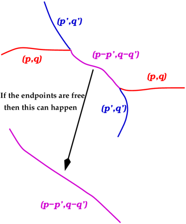
Figure 13: If the endpoints of the $(p,q)$ and $(p^{\prime},q^{\prime})$ strings are free then for example, a $(p-p^{\prime},q-q^{\prime})$ string can “zip up” the other strings and form a single $(p-p^{\prime},q-q^{\prime})$ string.

Colliding $(p,q)$ and $(p^{\prime},q^{\prime})$ strings do not generally annihilate and produce a daughter. Instead a 3-string vertex is usually created where the $(p,q),(p^{\prime},q^{\prime})$ and $(p\pm p^{\prime},q\pm q^{\prime})$ strings meet. See figure 1. If the endpoints of the $(p,q)$ and $(p^{\prime},q^{\prime})$ strings are free (not attached to other 3-string vertices) then it is energetically favorable for the two strings to move toward each other, merge, dissolve into each other and form a $(p\pm p^{\prime},q\pm q^{\prime})$ string. Thus $(p,q)+(p^{\prime},q^{\prime})\rightarrow(p\pm p^{\prime},q\pm q^{\prime})$ only occurs if the initial two strings are not part of a web such that their endpoints are free. See figure 13.

If two strings can merge and coalesce into one string after a collision quickly, and do so far before the next string collision, then a web may not form - i.e. $\tau_{merge}\ll\tau_{collision}$. The strings will on average then be non-intersecting. What can conceivably then happen is the following. A gas of strings with initially widely varying $p$ and $q$ can collide and self-intersect. It will be energetically favorable for the collisions to lead to lighter daughter strings. Thus, in the long term almost all of the strings will be the lightest possible strings, either $(\pm 1,0)$ or $(0,\pm 1)$, $\pm(1,1)$ or $\pm(1,-1)$ strings. These remaining strings may then self-intersect, form loops, and scale individually. Then $\Omega_{cs}=\Omega_{(\pm 1,1)}+\Omega_{(1,\pm 1)}+\Omega_{(\pm 1,0)}+\Omega_{(0,\pm 1)}$. If each of the $\Omega_{(p,q)}$ is small then $\Omega_{cs}$ will be small and the strings will not cause the universe to close.

A recent simulation by Tye, Wasserman and Wyman simulated such a string gas [42]. They assumed the endpoints of the strings were free and the lengths of all the strings were the same. This allowed them to assume that once a $(p,q)$ and a $(p^{\prime},q^{\prime})$ string collide, they annihilate and form a $(p\pm p^{\prime},q\pm q^{\prime})$ string. They used essentially the same equation as the Velocity One Scale model in equation (112) for each $(p,q)$ species of string. For convenience, we denote each $(p,q)$ species by $\alpha$ such that $\alpha\equiv(p,q)$. They wrote a version of (112) using the number density $n_{\alpha}$.

$$\dot{n}_{\alpha}=-2\frac{\dot{a}}{a}n_{\alpha}-\frac{c_{2}n_{\alpha}v}{L}-\tilde{P}n_{\alpha}^{2}vL+FvL\left(\sum_{\beta,\gamma}P_{\alpha\beta\gamma}n_{\beta}n_{\gamma}\frac{(1+\delta_{\beta\gamma})}{2}-\sum_{\beta,\gamma}P_{\beta\gamma\alpha}n_{\gamma}n_{\alpha}(1+\delta_{\gamma\alpha})\right)$$ (117)

This can be rephrased in terms of the energy density by using $\rho_{\alpha}=(1-v^{2})^{-1/2}\mu_{\alpha}n_{\alpha}$ and the velocity evolution equation (114) with $k/R$ replaced by $c_{2}/L$. Thus $c_{2}$ represents the momentum parameter $k$ and $R$ is taken to be the correlation length $L$.

On the right hand side of (117), the second term represents string loss via loop production from string self-intersections. The third term represents string loss from the collision of strings of the same type. $L$ appears to make the dimensions correct. $\tilde{P}$ is the probability that a collision of strings of the same type will create a loop of $\alpha$ string.

The fourth term represents the process $\beta+\gamma\rightarrow\alpha$. $F$ is the “overall interaction probability” of the process. The $vL$ appear for the same reasons as previously mentioned. $P_{\alpha\beta\gamma}$ is the branching ratio for a $\beta$ and $\gamma$ string to become an $\alpha$ string. The $1/2$ appears because of double-counting since the sum is symmetric in $\beta$ and $\gamma$. However, the diagonal term $n_{\beta}^{2}P_{\alpha\beta\beta}$ occurs only once. To insure that it occurs twice so that $\frac{1}{2}$ (two occurrences) = 1 occurrence, Tye Wasserman and Wyman insert the factor $(1+\delta_{\beta\gamma})$.

The fifth term represents the process $\alpha+\gamma\rightarrow\beta$ and appears with a minus sign because one $\alpha$ string is destroyed. The diagonal term in the sum $n_{\alpha}^{2}P_{\beta\alpha\alpha}$ represents the loss of two $\alpha$ strings. That is why the sum must be corrected with the factor $(1+\delta_{\gamma\alpha})$.

The branching ratio $P_{\alpha\beta\gamma}$ can be estimated as follows. As shown in $\S\ref{sectionpq}$, the critical angle determining whether a $(p+p^{\prime},q+q^{\prime})$ string or a $(p-p^{\prime},q-q^{\prime})$ string will form is given by (15).

$$\cos\theta_{c}=\frac{{\mbox{\boldmath$\mu_{(p,q)}\cdot\mu_{(p^{\prime},q^{\prime})}$}}}{{\mbox{\boldmath$|\mu_{(p,q)}||\mu_{(p^{\prime},q^{\prime})}|$ }}}=\frac{pp^{\prime}+g_{s}^{-2}qq^{\prime}}{\sqrt{p^{2}+g_{s}^{-2}q^{2}}\sqrt{p^{\prime 2}+g_{s}^{-2}q^{\prime 2}}}$$ (118)

where we have chosen the “+” sign in (15). For $\theta<\theta_{c}$ a $(p+p^{\prime},q+q^{\prime})$ string may form. For $\theta>\theta_{c}$ only a $(p-p^{\prime},q-q^{\prime})$ string can form. The possible range of $\cos\theta$ is $[-1,1]$. If any value of $\theta$ is equally likely then the probability ${\mathbb{P}}(\cos\theta)$ is $1/2$. Thus the probability ${\mathbb{P}}(\cos\theta>\cos\theta_{c})=(1-\cos\theta_{c})/2$ and ${\mathbb{P}}(\cos\theta<\cos\theta_{c})=(1+\cos\theta_{c})/2$. Thus if $\beta=(p,q)$ and $\gamma=(p^{\prime},q^{\prime})$,

$$P_{\beta+\gamma,\beta\gamma} = \frac{1}{2}\left(1-\frac{pp^{\prime}+g_{s}^{-2}qq^{\prime}}{\sqrt{p^{2}+g_{s}^{-2}q^{2}}\sqrt{p^{\prime 2}+g_{s}^{-2}q^{\prime 2}}}\right)$$ (119)

$$P_{\beta-\gamma,\beta\gamma} = \frac{1}{2}\left(1+\frac{pp^{\prime}+g_{s}^{-2}qq^{\prime}}{\sqrt{p^{2}+g_{s}^{-2}q^{2}}\sqrt{p^{\prime 2}+g_{s}^{-2}q^{\prime 2}}}\right)$$ (120)

Some properties of (119) are: if $\beta=(p,q)$ the probability of creating a $\beta+\beta=(2p,2q)$ string is zero since $P_{2\beta,\beta\beta}=0$. This is because the daughter $(2p,2q)$ string is not actually a bound state since $2\sqrt{p^{2}+q^{2}/g_{s}^{2}}=\sqrt{(2p)^{2}+(2q)^{2}/g_{s}^{2}}$. Hence $(2p,2q)$ strings are not long-lived and can decay back to two $(p,q)$ strings. I.e., identical strings either collide and pass through each other and in the long run remain as two identical strings or they form loops; they do not create heavier strings. In a similar way the process $(p,q)+(p^{\prime},q^{\prime})\rightarrow(Nk,Nl)$ doesn’t happen because an $(Nk,Nl)$ state is not a boundstate. There is nothing to prevent the $(Nk,Nl)$ string from decaying to $N$ $(k,l)$ strings because $\mu_{(Nk,Nl)}=N\mu_{(k,l)}$ (if $k$ and $l$ are relatively prime). Hence, one must be careful how one inserts $P_{\alpha\beta\gamma}$ into (117). Tye Wasserman and Wyman therefore take $P_{(Nk,Nl)(p,q)(p^{\prime},q^{\prime})}=NP_{(k,l)(p,q)(p^{\prime},q^{\prime})}$ if $(p\pm p^{\prime},q\pm q^{\prime})=(Nk,Nl)$.

Also note that the process $\beta+\beta\rightarrow(0,0)$ corresponds to loop formation from same type collisions and $P_{0\beta\beta}$ using (120). (A string with $(p,q)=(0,0)$ is a closed string loop). However, this process is already taken into account by the second term in (117). Thus to prevent this interaction from appearing twice in (117) we set $P_{0\beta\beta}=0$ by hand.

Using (119), (120) inserted into (117), Tye Wasserman and Wyman simulated a gas of interacting $(p,q)$ strings in 3+1 dimensions. They chose widely varying initial conditions for the number of each type of $(p,q)$ strings in the string gas and found that initial conditions were largely irrelevant. Numerically, they found that for most reasonable values of $P\mathrel{\hbox to0.0pt{\lower 4.0pt\hbox{\hskip 1.0pt$\sim$}\hss}\raise 1.0pt\hbox{$<$}}F\neq 0$ that the string network scaled, the number of strings with large $p$ or $q$ was suppressed and that most of the string energy was concentrated in the lowest tension $(\pm 1,0)$ or $(0,\pm 1)$, $\pm(1,1)$ or $\pm(1,-1)$ strings.

For $F\gg\tilde{P}$ they found that the number densities of higher tension strings were highly suppressed. This is expected since string collisions ($F$ interactions) tend to lower $p$ and $q$.

For $P\sim F$, they found that the number of higher tension strings, $N_{(p,q)}$ was roughly power law suppressed as $N_{(p,q)}\propto\mu_{(p,q)}^{-n}$ with $6<n\;\raise 1.72218pt\hbox{$<$}\kern-8.00003pt\lower 2.6694pt\hbox{$\sim$}\;10$. The strings reach an approximate scaling solution where for example, $\frac{\Omega_{(0,1)}}{\frac{8}{3}\pi G\mu_{(0,1)}}=\frac{46}{F+0.53P}$ for $g_{s}=1/2$. The scaling is approximate because the strings continue to evolve at late times. However, they claim that this late evolution is not cosmologically problematic.

For $F\rightarrow 0$, they found that each $(p,q)$ species scaled individually. Higher tension strings were not suppressed and $\Omega_{(p,q)}/\mu_{(p,q)}$ for each $(p,q)$ species converged to the same value leading to possible disaster since $\sum_{p,q}^{\infty}\Omega_{(p,q)}$ may explode.

Unfortunately, the authors do not present results for realistic case of $g_{s}\ll 1$. The authors show that for $g_{s}=1$, F and D-strings are interchangeable as expected. They also show that for $g_{s}=0.5$ that the number of F-strings is 2-3 times the number of D-strings. It would be nice to know for say $g_{s}\sim 1/10$ whether $D$-strings and $(p,q)$ strings with $q>1$ are power law suppressed like the heavier $(p,q)$ strings and/or whether they scale individually. It would also be helpful to understand what happens when both $F$ and $P$ are very small since $F,P\sim g_{s}^{2}\ll 1$.

7.3 Using the $D$ dimensional VOS model with F and D strings

Unfortunately, string physics is more complicated than the previous section’s approach. Classically ($g_{s}\ll 1$) strings will evolve only on a 3+1 dimensional slice of the higher dimensional spacetime [70, 69]. However, quantum mechanically they will wander off this slice and move in the extra dimensions. If the strings form at the bottom of a throat with significant redshifting, they will be localized at the bottom of the throat. Unless they are localized in the compact directions by a confining potential they will be able to move longitudinally and explore the extra-dimensional space at the throat bottom which for the special case of a deformed conifold throat is an $S^{3}$ (assuming no $SU(2)\times SU(2)$ breaking).

Motion in the extra dimensions leads to the following interesting consequences. (1) Moving strings generically intersect in 3+1 dimensions. In higher dimensions, they miss each other as non-interacting $p$ dimensional objects generically collide in $d$-dimensional spacetimes only if $d\leq 2(p+1)$ [106]. (2) If the extra dimensions are fixed, the extra dimensional velocities do not redshift. Cosmic strings in expanding universes are constrained by $v^{2}\leq 1/2$. Hence, if extra dimensional velocities grow then 3+1 dimensional velocities must decrease. This may happen because while extra-dimensional and 4D velocities have similar sized source terms, the 4D velocities are redshifted away while the extra-dimensional velocities build up. All the velocity may end up in the extra dimensions. The strings will then stop moving in the large dimensions. They will not scale because loop forming collisions will be infrequent and they will be unable to discharge their growing lengths/energies. Avgoustidis and Shellard (AS) recently analyzed these consequences of string propagation in extra dimensions [43].

AS started with a metric of the form

$$ds^{2}=N(t)^{2}dt^{2}-a(t)^{2}d\mbox{\boldmath$x$}^{2}-b(t)^{2}d{\mbox{\boldmath$y$}}^{2}$$ (121)

which is isotropic in 3 large spatial directions and separately isotropic in $D-3$ small extra dimensions ($D$ is the number of spatial dimensions). Note, no warping appears in the metric. The inclusion of $N(t)$ allows one to switch between physical and conformal time very easily. If $N=1$ then $t$ is the physical time. If $N=a=b$ then $t$ is very conveniently the conformal time.

After deriving the equations of motion and expression for the energy AS wrote down how the energy redshifts over time

$$\dot{\rho}=-\frac{\dot{a}}{a}\left(2(1+v_{x}^{2})+v_{y}^{2}+W_{1}\right)\rho-\frac{\dot{b}}{b}\left[(D-4+v_{y}^{2})+v_{x}^{2}+W_{2}\right]\rho$$ (122)

This is a very similar to (112). Compared to (112) the first term on the right has an extra term $v_{y}^{2}+W_{1}$. This represents the effects of extra dimensions and extra-dimensional velocities. Note, even if the extra-dimensional velocity vanishes, $v_{y}=0$, and the extra dimensions are fixed, $\dot{b}=0$, (122) differs from the 4D VOS model.

In the second term $(D-4)/2$ instead of ”2” appears because while the codimension of strings in 3 spatial dimensions is 2, the codimension of a string in $D-3$ extra dimensions is $(D-3)-1$. Otherwise the two terms are interchangeable because under the exchange of $(a,\mbox{\boldmath$x$})\rightarrow(b,\mbox{\boldmath$l$})$, we have $W_{1}\rightarrow W_{2}$.

The velocities, $v_{x},v_{y}$ have been defined to be

$$v_{x}^{2}=\left\langle\frac{a^{2}}{N^{2}}\dot{\mbox{\boldmath$X$}}^{2}\right\rangle v_{y}^{2}=\left\langle\frac{b^{2}}{N^{2}}\dot{\mbox{\boldmath$Y$}}^{2}\right\rangle$$ (123)

where the averaging is done as

$$\langle f\rangle=\frac{\int f\epsilon d\sigma^{1}}{\int\epsilon d\sigma^{1}}$$ (124)

and $\epsilon$ is the energy per unit string length. The $W$ functions are defined as

$$W_{1}\!\! = \!\!\left\langle\frac{b^{2}\mbox{\boldmath$Y$}^{\prime 2}}{a^{2}\mbox{\boldmath$X$}^{\prime 2}\!\!+b^{2}\mbox{\boldmath$Y$}^{\prime 2}}\frac{N^{2}\!-\!a^{2}\dot{\mbox{\boldmath$X$}}^{2}\!\!-\!b^{2}\dot{\mbox{\boldmath$Y$}}^{2}}{N^{2}}\right\rangle\approx\left\langle\frac{b^{2}\mbox{\boldmath$Y$}^{\prime 2}}{a^{2}\mbox{\boldmath$X$}^{\prime 2}+\mbox{\boldmath$Y$}^{\prime 2}}\right\rangle(1\!-\!v_{x}^{2}\!-\!v_{y}^{2})$$ (125)

$$W_{2}\!\! = \!\!\left\langle\frac{a^{2}\mbox{\boldmath$X$}^{\prime 2}}{a^{2}\mbox{\boldmath$X$}^{\prime 2}\!\!+\!b^{2}\mbox{\boldmath$Y$}^{\prime 2}}\frac{N^{2}\!-\!a^{2}\dot{\mbox{\boldmath$X$}}^{2}\!\!-\!b^{2}\dot{\mbox{\boldmath$Y$}}^{2}}{N^{2}}\right\rangle\approx\left\langle\frac{a^{2}\mbox{\boldmath$X$}^{\prime 2}}{a^{2}\mbox{\boldmath$X$}^{\prime 2}\!+\!\mbox{\boldmath$Y$}^{\prime 2}}\right\rangle(1\!-\!v_{x}^{2}\!-\!v_{y}^{2})$$ (126)

On the L.H.S we have used the approximation that worldsheet spatial derivative terms like $f^{\prime}$ are uncorrelated with worldsheet time terms like $\dot{f}$. $W_{1}$ and $W_{2}$ are related to the amount of string that lies in the extra and 3+1 dimensions respectively.

If the extra dimensions are fixed such that $b=1$ then we will call $W_{1}(b=1)=w_{ls}(1-v_{x}^{2}-v_{y}^{2})$. $w_{ls}$ measures the proportion of the string in the extra dimensions. Equation (122) becomes

$$\dot{\rho}=-\frac{\dot{a}}{a}\left[(2+w_{ls})+(2-w_{ls})v_{x}^{2}+(1-w_{ls})v_{y}^{2}\right]\rho$$ (127)

Note, even if $v_{y}=0$, (127) differs from the 4D VOS model of (112) because of $w_{ls}$.

If we assume that on average the partitioning of gradient energy in $w_{ls}$ = (gradient energy in $\mbox{\boldmath$Y$}^{\prime 2}$)/(total gradient energy), is equal to the partitioning of kinetic energy in (KE in $\dot{\mbox{\boldmath$Y$}}^{2}$)/(total KE), then we can model $w_{ls}$ as

$$w_{ls}=\left\langle\frac{\mbox{\boldmath$Y$}^{\prime 2}}{a^{2}\mbox{\boldmath$X$}^{\prime 2}+\mbox{\boldmath$Y$}^{\prime 2}}\right\rangle\simeq\left\langle\frac{\dot{\mbox{\boldmath$Y$}}^{2}}{a^{2}\dot{\mbox{\boldmath$X$}}^{2}+\dot{\mbox{\boldmath$Y$}}^{2}}\right\rangle=\frac{v_{y}^{2}}{v^{2}}$$ (128)

Note, in this approximation if $v_{y}=0$ then $w_{ls}=0$ and (112) coincides with the $D+1$ dimensional VOS model (127).

AS argue that if the correlation length $L$ of the strings is much larger than the size of the extra dimensions then string motion is effectively 3-dimensional, and $\rho=\mu/L^{2}$ instead of say $\rho=\mu L^{-2}L^{-(D-3)}$. Even if this is not initially true, if the strings scale such that $L=\gamma t$, then $L$ will eventually grow larger than the size of the (fixed) extra dimensions. Inputting $L=\gamma(t)t$ and $\rho=\mu/L^{2}$ and $w_{ls}=v_{y}^{2}/v^{2}$ into (127) yields

$$\frac{\dot{\gamma}}{\gamma}=\frac{1}{2t}\left(\beta(2+2v_{x}^{2}+v_{y}^{2}/v^{2})-2+\frac{Pcv_{x}}{\gamma}\right)$$ (129)

The evolution equations for $v_{x}$ and $v_{y}$ under the same approximations are as copied out of AS

$$\frac{\dot{v}_{x}}{v_{x}} = \frac{1}{t}\left(\frac{k_{x}v_{x}}{\gamma}(1-v^{2})-\beta v_{x}^{2}(2-2v_{x}^{2}-v_{y}^{2}/v^{2})\right)$$ (130)

$$\frac{\dot{v}_{y}}{v_{y}} = \frac{1}{t}\left(\frac{k_{y}v_{y}}{\gamma}(1-v^{2})-\beta v_{y}^{2}(1-2v^{2})(1-v_{y}^{2}/v^{2})\right)$$ (131)

As before $k_{x}$ and $k_{y}$ are momentum parameters measuring how correlated the string curvature is with the directions of $v_{x}$ and $v_{y}$ respectively. $k_{x}$ and $k_{y}$ are related to $k$ by $kv=k_{x}v_{x}+k_{y}v_{y}$. The formal definitions of $k_{y}$ and $k_{x}$ are

$$\frac{k_{x}v_{x}(1\!-\!v^{2})}{R}\!=\!\langle\mbox{\boldmath$\dot{X}$}\cdot\mbox{\boldmath$u$}(1\!-\!\dot{\mbox{\boldmath$X$}}^{2}\!-\!\frac{\dot{\mbox{\boldmath$Y$}}^{2}}{a^{2}})\rangle\!\! \frac{k_{y}v_{y}(1\!-\!v^{2})}{R}\!=\!\langle\frac{\dot{\mbox{\boldmath$Y$}}}{a}\cdot\mbox{\boldmath$u$}(1\!-\!\dot{\mbox{\boldmath$X$}}^{2}\!-\!\frac{\dot{\mbox{\boldmath$Y$}}^{2}}{a^{2}})\rangle$$ (132)

If the string motion is effectively 3-dimensional, then the curvature vector $u$ will mostly lie along the 3 large dimensions making $\dot{\mbox{\boldmath$Y$}}\cdot\mbox{\boldmath$u$}\ll 1$ and $\mbox{\boldmath$\dot{X}$}\cdot\mbox{\boldmath$u$}\sim 1$ in (132). Thus $k_{x}\gg\ k_{y}$. Since the source term for $v_{x}$ is $\propto k_{x}$ from (130) and the source term for $v_{y}$ is $\propto k_{y}$ from (131), the source term for 3D velocities is much greater than for $v_{y}$. However, note from (130) and (131), that the damping term for $v_{x}$ is significantly greater than the damping term of $v_{y}$ because the extra dimensions do not expand.

Equation (129) was numerically solved for: (a) varying amounts of ”3Dness;” (b) varying initial $v_{y}$ and $v_{x}$; (c) varying intercommuting probability $P$.

Figure 14: From left to right: (1) Velocity evolution if the strings evolve in more than 3 dimensions such that $k_{x}\sim k_{y}$. Note here $v_{y}\equiv v_{\ell}$. For $D$ dimensional evolution $v_{y}\equiv v_{\ell}$ quickly dominates $v_{x}$ and the strings stop moving in the extra dimensions. (2) Evolution of $\gamma$ for 3D motion if $v_{y}\simeq 0.3$ initially. (3) $\gamma(t)$ if $v_{y}\simeq 0.95/\sqrt{2}$ initially.

If the motion of strings is not very 3-dimensional such that the curvature vector $u$ explores the extra dimensions and $k_{y}$ is not small then, $v_{x}^{2}\rightarrow 0$ and $v_{y}^{2}\rightarrow 1/2$. See the first graph in figure 14. This is because in this case $v_{x}$ and $v_{y}$ have similar source terms, but $v_{x}$ is more damped than $v_{y}$. Since $v_{x}^{2}+v_{y}^{2}\leq 1/2$, this means that $v_{y}$ grows relative to $v_{x}$ and drives $v_{x}\rightarrow 0$. As the loop production term is $\propto v_{x}$, loop production then ceases, no scaling solution is reached and strings presumably dominate the energy density of the universe.

For 3D motion, even if $v_{y}\,\,\raise 1.72218pt\hbox{$<$}\kern-8.00003pt\lower 2.6694pt\hbox{$\sim$}\,\,\frac{1}{\sqrt{2}}$ initially, a scaling solution is reached although the scaling value of $\gamma$ is smaller by a factor of 2 then were say $v_{y}=0.3$ initially, see figure 14. Since $\rho\sim\gamma^{-2}$, the string density is a factor of $4$ larger in the $v_{y}\simeq\frac{0.95}{\sqrt{2}}$ case compared to the $v\simeq 0.3$ case. Nevertheless, unlike the $D$ dimensional case, a scaling solution is reached in this 3D case because unlike the previous case, here $v_{x}$ is not driven to zero. It reaches the asymptotic value $v_{x}\approx 0.2$ for $v_{y}=0.95/\sqrt{2}$. See figure 14. For smaller initial values of $v_{y}$, $v_{x}$ quickly dominates $v_{y}$ because $k_{x}\gg k_{y}$.

Figure 15: Time evolution of the scaling parameter $\gamma$ for varying intercommuting probability $P$. From left to right $P=1,\;0.3,\;10^{-3}$. Even for $P=10^{-3}$ a scaling solution exists with $\gamma\simeq P$. However, it takes much longer to reach it.

For 3D motion the effects of small $P$ are not overwhelming. Even if $P\sim 10^{-3}$ and $v_{y}=0.36$ strings apparently still scale. However, the time needed to scale dramatically increases. See figure 15.

8 Gravitational Emission from Strings with Cusps

Cosmic strings strongly emit gravitational waves. It was assumed that the spectrum is Gaussian. Hence, for $G\mu<10^{-7}$ gravitational waves from strings were thought to be too weak to be detected. Recently Vilenkin and Damour showed that gravitational emission from cusps on cosmic strings is strongly non-Gaussian [24, 25, 26]. Hence even if $G\mu\sim 10^{-10}$, gravitational waves from strings are detectable by LIGO and LISA. Cosmic superstrings are distinguished from field theory strings because their intercommuting probability $P$ may be very small, while field theory strings always intercommute. The smaller $P$ is the stronger the gravitational wave signal is. It is therefore remarkable that not only may galaxy-sized superstrings be detectable, but they may be the ”brightest things in the sky” [10].

8.1 Cusp formation

The worldsheet metric $\gamma_{ab}$ is not unique. It is invariant under worldsheet reparameterizations, $(\sigma,\tau)\rightarrow(f_{\sigma}(\sigma,\tau),f_{\tau}(\sigma,\tau))$. The metric can be fixed by imposing gauge conditions. First, impose the gauge condition $\gamma_{00}+\gamma_{11}=0$. Since $\gamma_{ab}=\partial_{a}X^{\mu}\partial_{b}X_{\mu}$ this leads to $\dot{X}^{2}+X^{\prime 2}=0$. Next align worldsheet and physical time $\tau=t=X^{0}$. In this section we will ignore the extra dimensions and only work with the strings’ 3D properties. Hence, we take $X^{\mu}=(X^{0},\mbox{\boldmath$X$})$ where $X$ is a 3-vector. We also impose $\gamma_{01}=0$. This gives the two conditions

$$\mbox{\boldmath$\dot{X}$}^{2}+\mbox{\boldmath$X$}^{\prime 2} = 1$$ (133)

$$\mbox{\boldmath$\dot{X}$}\cdot\mbox{\boldmath$X$}^{\prime} = 0$$ (134)

We decompose the target space coordinates into left and right moving components, $\mbox{\boldmath$X$}(\sigma,\tau)=\frac{1}{2}[\mbox{\boldmath$X$}_{+}(\sigma_{+})+\mbox{\boldmath$X$}_{-}(\sigma_{-})]$ and $X^{0}_{\pm}=\sigma_{\pm}$ where $\sigma_{\pm}=\tau\pm\sigma$. Since $\partial_{\pm}=\frac{1}{2}(\partial_{\tau}\pm\partial_{\sigma})$, we have $\dot{\mbox{\boldmath$X$}}=(\partial_{+}+\partial_{-})\mbox{\boldmath$X$}=\frac{1}{2}(\dot{\mbox{\boldmath$X$}}_{+}+\dot{\mbox{\boldmath$X$}}_{-})$ and $\mbox{\boldmath$X$}^{\prime}=\frac{1}{2}(\dot{\mbox{\boldmath$X$}}_{+}-\dot{\mbox{\boldmath$X$}}_{-})$ where we defined $\dot{\mbox{\boldmath$X$}}_{\pm}\equiv\partial_{\pm}\mbox{\boldmath$X$}_{\pm}$ and $\dot{\mbox{\boldmath$X$}}=\partial_{\tau}\mbox{\boldmath$X$}$. The two gauge conditions then imply ${\dot{\mbox{\boldmath$X$}}_{+}}^{2}(\sigma_{+})={\dot{\mbox{\boldmath$X$}}_{-}}^{2}(\sigma_{-})=1$ or in 4-vector notation $(\dot{X}^{\mu}_{\pm})^{2}=0$. Hence, $\pm\dot{\mbox{\boldmath$X$}}_{+}(\sigma_{+})$ and $\pm\dot{\mbox{\boldmath$X$}}_{-}(\sigma_{-})$ live on the unit sphere and trace out closed curves since they are periodic with respect to $\sigma_{+}$ and $\sigma_{-}$. $\dot{\mbox{\boldmath$X$}}_{+}$ and $\dot{\mbox{\boldmath$X$}}_{-}$ will generically intersect on the sphere. In fact, because of the periodicity of $\mbox{\boldmath$X$}_{\pm}$, we find that $\int_{0}^{L}\dot{\mbox{\boldmath$X$}}_{\pm}d\sigma_{\pm}=0$ implying that neither curve can lie in a single hemisphere, making it nearly impossible for $\dot{\mbox{\boldmath$X$}}_{+}$ and $\dot{\mbox{\boldmath$X$}}_{-}$ not to intersect at some worldsheet point $(\sigma_{+}^{(c)},\sigma_{-}^{(c)})$. At the intersection point: $\dot{\mbox{\boldmath$X$}}_{+}(\sigma_{+}^{(c)})=\dot{\mbox{\boldmath$X$}}_{-}(\sigma_{-}^{(c)})$ and the string velocity is $\mbox{\boldmath$\dot{X}$}^{2}(\sigma_{+}^{(c)},\sigma_{-}^{(c)})=\frac{1}{4}[\dot{\mbox{\boldmath$X$}}_{+}(\sigma_{+}^{(c)})+\dot{\mbox{\boldmath$X$}}_{-}(\sigma_{-}^{(c)})]^{2}=1$. Such a point where parts of a massive string reach the speed of light are called cusps, and the string shape near the cusp is of the form $y^{3}=x^{2}$. The cusp is at the singular point $(x,y)=(0,0)$.

The importance of cusps is that they strongly emit radiation which is not exponentially damped in the mode number. String loops with a non-singular shape emit their energy as radiation. However, their spectral power, $P_{n}$ falls exponentially at large $n$, while for cusps $P_{n}$ falls as some negative power of $n$. Hence, high power observational signals from cuspless strings are observationally very difficult to observe. For strings with cusps however, such high power radiation is much easier to detect. Any detection of such a high power signal would be provocative circumstantial evidence for the existence of cosmic strings and depending on the shape of the observationally measured power spectrum – evidence of cosmic superstrings.

8.2 Gravitational waves from cusps

Below we give a detailed and hopefully transparent account of Vilenkin and Damour’s calculation of the gravitational wave amplitude from cosmic string cusps. More details can be found in Vilenkin and Damour’s original 3 papers, [24, 25, 26].

A gravitational wave in the linearized approximation satisfies

$$\Box\,\bar{h}_{\mu\nu}=-\,16\pi\,G\,T_{\mu\nu}\,,$$ (135)

which has a solution

$$\bar{h}_{\mu\nu}(\mbox{\boldmath$x$},t)=\frac{\kappa_{\mu\nu}(t-r,\mbox{\boldmath$n$})}{r}+{\cal O}\left(\frac{1}{r^{2}}\right)\,.$$ (136)

where

$$\kappa_{\mu\nu}(t-r,\mbox{\boldmath$n$})=4\,G\ \sum_{\omega}\ e^{-i\omega(t-r)}\,T_{\mu\nu}(\mbox{\boldmath$k$},\omega)\simeq 2\,G\,\ell\int\frac{d\omega}{2\pi}\ e^{-i\omega(t-r)}\ T_{\mu\nu}(\mbox{\boldmath$k$},\omega).$$ (137)

On the right hand side we took a high frequency limit (where cusps are most important) enabling the replacement of $\sum_{\omega}$ by $\int d\omega$. Note that $k^{\mu}_{m}=(\omega_{m},\mbox{\boldmath$k$}_{m})\equiv\omega_{m}(1,\,\mbox{\boldmath$n$})$, where $n$ is the direction of emission.

If we define the logarithmic Fourier component $\kappa(f)$ as

$$\kappa(f)\equiv|f|\,\widetilde{\kappa}(f)\equiv|f|\int dt\ e^{2\pi ift}\,\kappa(t)\,.$$ (138)

then $\kappa_{\mu\nu}(f)$ can be conveniently related to $T_{\mu\nu}(\mbox{\boldmath$k$},\omega)$ by

$$\kappa_{\mu\nu}(f,\mbox{\boldmath$n$})=2\,G\,\ell\,|f|\,T_{\mu\nu}(\mbox{\boldmath$k$},\omega)\,.$$ (139)

As the wave $h(f)$ propagates over cosmological distances it will be redshifted by the expansion of the universe. One can show that (136) still holds provided $r\rightarrow a(t)r$ and the frequency an observer measures today is replaced as $f\rightarrow(1+z)f$. Thus

$$\bar{h}_{\mu\nu}(f)=\frac{\kappa_{\mu\nu}[(1+z)f]}{a(t)r}\approx\kappa_{\mu\nu}[(1+z)f]\frac{1+z}{t_{0}z}$$ (140)

where we set $t=t_{0}=\textsf{today}$ and $a_{0}=a(t_{0})$, and employed the redshift relation for a flat matter dominated universe,

$$a_{0}r=3t_{0}\left(1-\frac{1}{\sqrt{1+z}}\right)\;\approx\;t_{0}\frac{z}{1+z}$$ (141)

The energy momentum tensor for a string is

$$T^{\mu\nu}(x)=\mu\int d\tau\,d\sigma(\dot{X}^{\mu}\,\dot{X}^{\nu}-X^{\prime\mu}\,X^{\prime\nu})\,\delta^{(4)}(x-X(\tau,\sigma))\,.$$ (142)

which for periodic motion in time has the Fourier transform

$$T_{\mu\nu}(\mbox{\boldmath$k$},\omega) = \frac{1}{{\cal{T}}}\ \int_{0}^{{\cal{T}}}dt\int d^{3}\mbox{\boldmath$x$}\,e^{i(\omega t-\mbox{\boldmath$k$}\cdot\mbox{\boldmath$x$})}\,T_{\mu\nu}(\mbox{\boldmath$x$},t)$$ (143)

$$= \frac{\mu}{{\cal{T}}}\ \int_{\sum^{\prime}}d\tau\,d\sigma(\dot{X}_{\mu}\,\dot{X}_{\nu}-X^{\prime}_{\mu}\,X^{\prime}_{\nu})\,e^{-ik\cdot X}$$

$$= \frac{\mu}{2{\cal{T}}}\ \int_{\sum^{\prime}}d\sigma_{+}\,d\sigma_{-}\,\dot{X}_{+}^{(\mu}\dot{X}_{-}^{\nu)}\,e^{-\frac{i}{2}(k_{m}\cdot X_{+}+k_{m}\cdot X_{-})}$$

$$= \frac{\mu}{2{\cal{T}}}\ I_{+}^{(\mu}I_{-}^{\nu)}\,.$$ (145)

Here ${\cal{T}}=2\pi/\omega_{1}=\ell/2$ is the ”fundamental” oscillation period of the string and $\ell$ is the length of the string. $\Sigma^{\prime}$ is the worldsheet strip swept out in one period. In the third line we moved to $\sigma_{\pm}$ coordinates. In the last line, $I^{\mu}_{\pm}$ is defined as

$$I_{\pm}^{\mu}(k_{m})\equiv\int_{0}^{\ell}d\sigma_{\pm}\dot{X}_{\pm}^{\mu}e^{-\frac{i}{2}k_{m}\cdot X_{\pm}}\,.$$ (146)

A cusp will form if there is some $\ell^{\mu}$ such that $\ell^{\mu}=\dot{X}_{+}^{\mu}(\sigma_{+}^{(c)})=\dot{X}_{-}^{\mu}(\sigma_{-}^{(c)})$. Recall that $\dot{X}_{\pm}^{\mu}(\sigma_{\pm}^{(c)})$ is null and hence $\ell^{\mu}$ must be null. $I_{\pm}^{\mu}$ will decrease exponentially unless the phase of $I_{\pm}^{\mu}$ possesses a saddle point such that $\partial_{\pm}(k_{m}\cdot X_{\pm})=0$. Since both $k_{m}$ and $X_{\pm}^{\mu}$ are null, a saddle point at the worldsheet point $(\sigma_{+}^{(c)},\sigma_{-}^{(c)})$, will exist if $k_{m}^{\mu}\propto\dot{X}_{\pm}^{\mu}(\sigma_{\pm}^{(c)})=\ell^{\mu}$. Since $k^{\mu}_{m}=\omega_{m}(1,\,\mbox{\boldmath$n$})$, and $\dot{X}_{\pm}^{\mu}=(1,\mbox{\boldmath$\dot{X}$}_{\pm})$, and $\mbox{\boldmath$\dot{X}$}^{2}_{\pm}=1=\mbox{\boldmath$n$}^{2}$, we find that $k_{m}^{\mu}=\omega_{m}\ell^{\mu}$. Note: motion of the cusp is parallel to the direction of emission (assuming a saddle point) since $\dot{X}^{\mu}(\sigma_{+}^{(c)},\sigma_{-}^{(c)})=\frac{1}{2}[\dot{X}_{+}^{\mu}(\sigma_{+}^{(c)})+\dot{X}_{-}^{\mu}(\sigma^{(c)}_{-})]=\frac{1}{2}[\ell^{\mu}+\ell^{\mu}]=\ell^{\mu}$.

To evaluate $I_{\pm}$ for a cuspy string we shift the origin of $\sigma_{\pm}$ so that $\sigma_{\pm}^{(c)}=0$, and the origin of $X^{\mu}$ so that $X^{\mu}(\sigma_{+}^{(c)},\sigma_{-}^{(c)})=0$. The Taylor expansions around $X^{\mu}_{\pm}(\sigma_{+}^{(c)},\sigma_{-}^{(c)})$ are

$$X_{\pm}^{\mu}(\sigma_{\pm})=\ell^{\mu}\,\sigma_{\pm}+\frac{1}{2}\ \ddot{X}_{\pm}^{\mu}\,\sigma_{\pm}^{2}+\frac{1}{6}\ X_{\pm}^{(3)\mu}\,\sigma_{\pm}^{3}\,,$$ (147)

$$\dot{X}_{\pm}^{\mu}(\sigma_{\pm})=\ell^{\mu}+\ddot{X}_{\pm}^{\mu}\,\sigma_{\pm}+\frac{1}{2}\ X_{\pm}^{(3)\mu}\,\sigma_{\pm}^{2}\,,$$ (148)

Differentiating the constraint $\dot{X}_{\pm}^{2}=0$ mentioned in the paragraph below (134) yields the relations $\dot{X}_{\pm}\cdot\ddot{X}_{\pm}=0$ and $\dot{X}_{\pm}\cdot{X}_{\pm}^{(3)}+\ddot{X}_{\pm}^{2}=0$. Therefore, at the cusp, one has $\ell\cdot\ddot{X}_{\pm}=0$ and $\ell\cdot X_{\pm}^{(3)}=-(\ddot{X}_{\pm})^{2}$. Thus the phase factor in (146) is

$$k_{m}\cdot X_{\pm}=\omega_{m}\ell_{\mu}\,X_{\pm}^{\mu}(\sigma_{\pm})=-\frac{\omega_{m}}{6}\ (\ddot{X}_{\pm}^{\mu})^{2}\,\sigma_{\pm}^{3}\,.$$ (149)

Inserting these results in . (146) leads to an expression of the form

$$I_{\pm}^{\mu}=\int d\,\sigma_{\pm}(\ell^{\mu}+\ddot{X}_{\pm}^{\mu}\,\sigma_{\pm}+\cdots)\,\exp\left(\frac{i\omega_{m}}{12}\ddot{X}_{\pm}^{2}\,\sigma_{\pm}^{3}\right)\,.$$ (150)

Around the saddle point,$(\sigma_{+}^{(c)},\sigma_{-}^{(c)})=(0,0)$ we have $I_{\pm}^{\mu}\simeq a_{\pm}\,\ell^{\mu}+b_{\pm}^{\mu}$. The leading order term is $a_{\pm}\,\ell^{\mu}$ and $b_{\pm}^{\mu}$ is the subleading term. Since $\kappa_{\mu\nu}\sim I_{+}^{(\mu}I_{-}^{\nu)}$, the leading-leading order term is $a_{+}a_{-}\ell^{\mu}\ell^{\nu}$ and the leading-subleading terms are $a_{+}\ell^{\mu}b^{\nu}$ and $a_{-}\ell^{\nu}b^{\mu}$. These 3 terms can be gauged away by a coordinate transformation under which $\kappa_{\mu\nu}\rightarrow\kappa_{\mu\nu}+k_{\mu}\,\xi_{\nu}+k_{\nu}\,\xi_{\mu}$ where $k^{\mu}=\omega\ell^{\mu}$. Thus, the leading order physical part of $\kappa_{\mu\nu}$ is $\kappa_{\mu\nu}\sim I_{+}^{(\mu}I_{-}^{\nu)}=b_{+}^{(\mu}b_{-}^{\nu)}$ with

$$b_{\pm}^{\mu}\!\simeq\!\ddot{X}_{\pm}^{\mu}\int d\,\sigma_{\pm}\,\sigma_{\pm}\,\exp\left(\frac{i}{12}\,\omega_{m}\,\ddot{X}_{\pm}^{2}\,\sigma_{\pm}^{3}\right)\!=\!\frac{\ddot{X}_{\pm}^{\mu}}{N_{\pm}^{2}}\int_{-\infty}^{\infty}\!\!\!\!d\,u_{\pm}\,u_{\pm}\,e^{{i\,{\rm sign}(m)u_{\pm}^{3}}}\!=\!i\,{\rm sign}(m)\frac{\ddot{X}_{\pm}^{\mu}}{N_{\pm}^{2}}\frac{2\pi}{3\Gamma(\frac{1}{3})}$$ (151)

Recall that $\omega_{m}=m\omega_{1}$. The integral depends on the sign of $m$. Here, $u_{\pm}=N_{\pm}\sigma_{\pm}$ where $N_{\pm}^{3}=|\omega_{m}|\ddot{X}_{\pm}^{2}/12$. Since most of the integral over $d\sigma_{\pm}$ comes from around the saddle point, $\sigma_{\pm}=0$, we extended the integration limits of $u_{\pm}$ to $\pm\infty$.

The logarithmic Fourier transform is real, independent of the sign of $m$ and is

$$\kappa^{\mu\nu}(f)\ \simeq\ -C\frac{G\mu}{(2\pi|f|)^{1/3}}\frac{\ddot{X}_{+}^{(\mu}\ddot{X}_{-}^{\nu)}}{(|\ddot{X}_{+}||\ddot{X}_{-}|)^{4/3}}\ \sim\ \frac{G\mu\ell}{\sqrt[3]{|f|\ell}}\ \Theta(\,\theta_{0}(f)-\theta\,)$$ (152)

where $C=\frac{4\pi(12)^{\frac{4}{3}}}{\left(3\Gamma\left(\frac{1}{3}\right)\right)^{2}}$ and we have estimated $|\ddot{X}_{\pm}|\sim 2\pi/\ell$. We could do this because $X^{\mu}_{\pm}$ has the Fourier expansion $X^{\mu}_{\pm}\sim\frac{\ell}{2\pi}\sum\frac{\alpha_{n}^{\mu}}{n}e^{2\pi in\sigma_{\pm}/\ell}$ which gives $|\ddot{\mbox{\boldmath$X$}}_{\pm}|^{2}=(\frac{2\pi}{\ell})^{2}\sum n^{2}|{\mbox{\boldmath$\alpha$}}_{\pm}|^{2}$. Thus for not very large $n$ we find $|\ddot{\mbox{\boldmath$X$}}_{\pm}|\sim\frac{2\pi}{\ell}$ since $1=|\mbox{\boldmath$\dot{X}$}_{\pm}|^{2}=\sum|{\mbox{\boldmath$\alpha$}}_{\pm}|^{2}$. The Heaviside $\Theta(\theta_{0}-\theta)$ function appears because as Damour and Vilenkin show: if the direction of emission, $k$, (the direction to the observer) is misaligned from the direction of motion of the cusp $\ell$, by more than an angle $\theta_{0}$, the emission amplitude is exponentially suppressed. For example, Damour and Vilenkin show that if $\mbox{\boldmath$k$}\nparallel{\mbox{\boldmath$\ell$}}$ by more than an angle $\theta_{0}\simeq(\frac{2}{|f|\ell})^{1/3}$ then $I_{\pm}^{\mu}$ doesn’t possess a saddle point and decays exponentially.

Note (152) crucially depends of the absolute value $|f|\propto|m|$ because the integrals in (151) depend on the sign of $m$. This absolute value dependence is what causes distinctive “spikiness” of gravitational emission from cusps. Also note that because the vectors $\ddot{X}_{\pm}/|\ddot{X}_{\pm}|^{4/3}$ are spacelike and orthogonal to $\ell^{\mu}$, that gravitational wave in (152) is linearly polarized.

From now on we will usually assume that the observed frequency $f$ is positive and will thus drop the absolute value signs. Using (152) and (141), the wave amplitude $h(f)$ for a flat matter-dominated universe is

$$h(f)\sim\frac{G\mu\ell}{\sqrt[3]{(1+z)f\ell}}\;\frac{1+z}{t_{0}z}\;\Theta\left(\theta_{0}(f,z)-\;\;\theta\right)$$ (153)

Cosmic string loops will have a size of order the correlation length of the string network which is $L$. If the strings scale such $L\sim t$ is a fixed proportion of the horizon size $t$, then the loop size $\ell$ will be $\ell=\alpha t$. We define $\alpha=\epsilon\Gamma G\mu$ where $\Gamma\sim 50$ and $\epsilon$ are dimensionless numbers. $\epsilon$ measures how close $\alpha$ is to $\Gamma G\mu$. A very wiggly string with lots of small-scale structure may have a very small $\epsilon\sim 10^{-10}$. Smooth strings correspond to $\epsilon\sim 1$. Since $\ell\sim t$, and we would like to express (153) in terms of the redshift $z$, we need $t$ as a function of $z$. This is a complicated function because $a(t)$ takes different functional forms during the matter and radiation epochs. An approximate interpolating function relating $z$ to $t$ in both epochs is $t=t_{0}\varphi_{\ell}$ where $\varphi_{\ell}(z)=(1+z)^{-3/2}(1+z/z_{eq})^{-1/2}$. If for convenience, we define the new function $\varphi_{h}(z)=[\varphi_{\ell}(z)]^{2/3}z^{-1}(1+z)^{2/3}$ then we can write

$$h(f)\sim\frac{G\mu\alpha^{2/3}}{\sqrt[3]{ft_{0}}}\;\varphi_{h}(z)\;\Theta\left(\theta_{0}(f,z)\;-\;\theta\right)$$ (154)

where $f\rightarrow f(1+z)$ and $t=t_{0}\varphi_{\ell}$.

$$\theta_{0}=\frac{1}{\sqrt[3]{\alpha ft_{0}(1+z)\varphi_{\ell}}}=\frac{(1+z)^{1/6}(1+z/z_{eq})^{1/6}}{\sqrt[3]{\alpha ft_{0}}}$$ (155)

We would like to understand how $h(f)$ depends on the burst rate $\dot{N}$ for gravitational waves from cosmic strings. The burst rate changes with redshift as

$$\frac{d\dot{N}}{dz}\sim\frac{\theta_{0}^{2}}{4}(1+z)^{-1}\frac{cn_{\ell}}{{\cal{T}}}\frac{dV}{dz}$$ (156)

We understand (156) as follows. The number of bursts per string oscillation period $c$, divided by the string period ${\cal{T}}$, gives the number of cusps produced per unit time, $c/{\cal{T}}$. Multiplying that by the density of loops $n_{\ell}$, gives the (number of cusps)/(spacetime volume). Multiplying that by $dV(z)$, the spacetime volume in the interval $(z+dz,dz)$, gives the number of cusps produced between redshifts $z+dz$ and $z$ – this is $cn_{\ell}{\cal{T}}^{-1}dV(z)$. We now multiply by the fraction of cusps whose motion is in the same direction as an earthbound observer, ($\theta<\theta_{0}$). This is the amount of solid angle subtended by a cone with opening angle $\theta_{0}$. Since $\theta_{0}$ is small, this is approximately $\pi\theta_{0}^{2}/(4\pi)=\theta_{0}^{2}/4$. Finally, since $\dot{N}$ is a rate, and observed time redshifts as, $dt_{obs}=(1+z)dt$, we must multiply by $(1+z)^{-1}$.

For a flat universe,

$$\frac{dV}{dz}=\left\{\begin{array}[]{cc}54\pi t_{0}^{3}[(1+z)^{1/2}-1]^{2}(1+z)^{-11/2}&z<z_{eq}\\ 72\pi t_{0}^{3}(1+z_{eq})^{1/2}(1+z)^{-5}&z>z_{eq}\\ \end{array}\right\}$$ (157)

The loop density $n_{\ell}$ is the number of strings in a correlation length volume, $L^{3}\sim t^{3}=(t_{0}\varphi_{\ell})^{3}$. In order for strings to scale, long strings must release their energy in the form of loops. If all the length in a correlation volume were to go to loops, then the number of loops formed per time $t\sim L$ and per volume $L^{3}$ would be $\frac{L(t)}{\ell(t)}$. This implies that at least $\frac{L(t)}{\ell(t)}$ collisions/self-intersections are required. However, if probability of a collision leading to the formation of a loop is $P$, then more collisions are needed for the strings to scale. In particular, $1/P$ times more collisions are required. This can only happen if there are at least $1/P$ strings per $L^{3}$, instead of just 1 string per $L^{3}$. Then the number of loops needed for scaling is $N_{s}\sim\frac{1}{P}\frac{L(t)}{\ell(t)}\sim\frac{1}{P\alpha}$ using $L\sim t,\ell=\alpha t$. The lifetime of a loop is $\tau\sim\epsilon t$. Thus, the number of strings which survive till time $t$ is $\frac{\tau}{t}N_{s}$. Hence the loop density at time $t$ is then $n_{\ell}\sim\frac{\epsilon}{P\alpha}t^{-3}$. (Note the energy density goes as $n_{\ell}\ell\sim\mu/Pt^{2}\equiv\mu/L^{2}$ if $\epsilon=1$ implying that the scaling solution is $L\sim\sqrt{P}t$.)

If we plug in $n_{\ell}$, the period ${\cal{T}}=\frac{\ell}{2}=\frac{\alpha t_{0}\varphi_{\ell}}{2}$, and equations (155) and (157) into (156), we get a piecewise very complicated function. But, by introducing a new interpolating function $\varphi_{n}(z)=z^{3}(1+z)^{-7/6}(1+z/z_{eq})^{11/6}$ we can write a simpler expression for $d\dot{N}/dz$:

$$\frac{d\dot{N}}{d\ln z}\sim\frac{100\epsilon c}{Pt_{0}\alpha^{8/3}}\frac{\varphi_{n}(z)}{(ft_{0})^{2/3}}$$ (158)

$\varphi_{n}(z)$ is a strongly increasing function and varies as $z^{11/3}$ for large $z$. Thus $d\dot{N}/d\ln z$ is strongly peaked at large $z$. If $z_{m}$ is the largest allowed redshift, then we can approximate

$$\dot{N}=\int^{z_{m}}\left(\frac{d\dot{N}}{d\ln z}\right)d\ln z\approx\frac{d\dot{N}}{d\ln z}(z_{m})$$ (159)

Thus using (158) and (159), we can write

$$\varphi_{n}(z_{m})=10^{-2}\frac{P\dot{N}}{\epsilon c}t_{0}\alpha^{8/3}(ft_{0})^{2/3}\equiv y(\dot{N},f)$$ (160)

Note, the L.H.S of (160) depends on only $z_{m}$, while the R.H.S is a function of only $\dot{N}$ and $f$. We call this function $y(\dot{N},f)$. Equation (160) can thus be inverted. We can then write the maximum redshift $z_{m}$ as a function of the observed $\dot{N},f$ as

$$z_{m}(y)=y^{1/3}(1+y)^{7/33}(1+y/y_{eq})^{-3/11}$$ (161)

with $y$ given by (160). Note, if $y<1\Rightarrow z_{m}<1$, if $1<y<y_{eq}\Rightarrow 1<z_{m}<z_{eq}$, and if $y>y_{eq}\Rightarrow z_{m}>z_{eq}$ where $y_{eq}=z_{eq}^{11/6}$. We can then stick $z_{m}$ into (154), and $\theta_{0}(z,f)$ to get an expression for the wave amplitude for given values of $\dot{N}$ and $f$. The dependence on $z$ has thus been replaced by the dependence on $\dot{N}$ and $f$. Thus,

$$h(f,\dot{N},y)=G\mu\alpha^{2/3}\frac{g(y)}{\sqrt[3]{ft_{0}}}\Theta(\theta_{0}-\theta)=\Gamma^{2/3}(G\mu)^{5/3}\epsilon^{2/3}\frac{g(y)}{\sqrt[3]{ft_{0}}}\Theta(\theta_{0}-\theta)$$ (162)

where on R.H.S, we have replaced $\alpha$ by $\alpha=\epsilon\Gamma G\mu$ and where

$$g[y(\dot{N},f)]=\varphi_{h}(z_{m}(y))=y^{-1/3}(1+y)^{-13/33}(1+y/y_{eq})^{3/11}$$ (163)

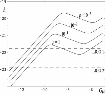
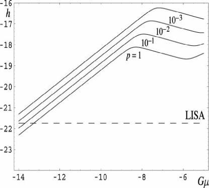
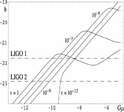
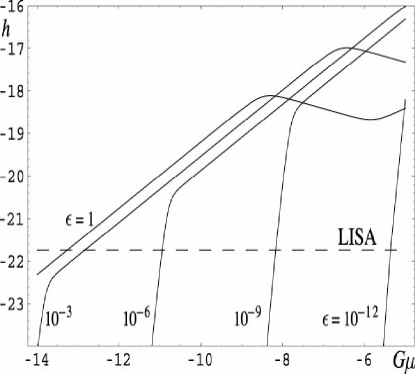
Figure 16: Log-log plots of $h(f)$ versus $G\mu$. Starting from top left: (1) at $f_{LIGO}=150$ Hz for $10^{-3}\leq P\leq 1$; (2) at $f_{LISA}=3.88\cdot 10^{-3}$ Hz for $10^{-3}\leq P\leq 1$; (3) at $f_{LIGO}$ for $10^{-12}\leq\epsilon\leq 1$; (4) at $f_{LISA}$ for $10^{-12}\leq\epsilon\leq 1$.

Figure 16 shows log-log plots of $h(f)$ versus $G\mu$ for: (1) $f=f_{LIGO}=150$ Hz for $1\leq P\leq 10^{-3}$; (2) $f=f_{LISA}=3.88\cdot 10^{-3}$ Hz for $1\leq P\leq 10^{-3}$; (3) $f=f_{LIGO}=150$ Hz for $10^{-12}\leq\epsilon\leq 1$; and (4) $f=f_{LISA}=3.88\cdot 10^{-3}$ Hz for $10^{-12}\leq\epsilon\leq 1$. All the plots assumed $c=1$, i.e. that one cusp per period was produced and that $\dot{N}=1/year$. The burst amplitude rises as $G\mu$ becomes larger than $10^{-12}$. Then it falls and then rises again. The local maximum and minimum depend on $f,p$ and $\epsilon$.

The dependence of $h(f)$ on $G\mu$ is understood as follows. Now from (160), $y\sim(G\mu)^{8/3}$. Also, $h(f,y)\sim(G\mu)^{5/3}g(y)$ has the power law behavior $h\sim(G\mu)^{5/3}g\sim(G\mu)^{5/3}y^{n}$ where $n=-1/3,-8/11,-5/11$ for $y\mathrel{\hbox to0.0pt{\lower 4.0pt\hbox{\hskip 1.0pt$\sim$}\hss}\raise 1.0pt\hbox{$<$}}1$, $1\mathrel{\hbox to0.0pt{\lower 4.0pt\hbox{\hskip 1.0pt$\sim$}\hss}\raise 1.0pt\hbox{$<$}}y\mathrel{\hbox to0.0pt{\lower 4.0pt\hbox{\hskip 1.0pt$\sim$}\hss}\raise 1.0pt\hbox{$<$}}y_{eq}$ and $y\mathrel{\hbox to0.0pt{\lower 4.0pt\hbox{\hskip 1.0pt$\sim$}\hss}\raise 1.0pt\hbox{$>$}}y_{eq}$ respectively. Thus $h\sim(G\mu)^{k}$ where $k=7/9,-3/11,5/11$ for $0<z_{m}<1$, $1<z_{m}<z_{eq}$, and $z>z_{eq}$.

$G\mu$ measures the radiation power of the string. So it is not surprising that apart from the middle regime $1<z_{m}<z_{eq}$ that the burst amplitude increases with $G\mu$. However, the loop density varies as $(G\mu)^{-1}$; hence the number of radiation emitting loops decreases with increasing $G\mu$. For $z_{m}<1$ and $z_{m}>z_{eq}$, the radiation power effect dominates the loop density effect. However, in the middle regime, the two effects are comparable and the fact that fewer loops are produced is actually more important than the increase in radiation power. Hence, for $1<z_{m}<z_{eq}$ the burst amplitude decreases with increasing string gravity, $G\mu$.

The dependence on $P$ and $\epsilon$ is explained as follows. Since $y\sim P\epsilon^{5/3}$, we find $h(f)\sim\epsilon^{2/3}(P\epsilon^{5/3})^{n}\sim P^{n}\epsilon^{(2+5n)/3}$. Therefore the $\epsilon,P$ dependence is $h\sim P^{-1/3}\epsilon^{1/9}$ and $P^{-8/11}\epsilon^{-6/11}$ and $P^{-5/11}\epsilon^{-1/11}$ for the three regimes respectively.

Thus decreasing $P$ increases $h$ slightly. If $P$ decreases to $P=10^{-3}$, $h$ increases by an order of magnitude. The dependence on $\epsilon$ is very weak, and unless $\epsilon$ decreases to $10^{-10}$, $h(f)$ hardly changes. However, if $G\mu\sim 10^{-10}$ as in the KKLMMT scenario, then taking $\epsilon\rightarrow 10^{-10}$ takes $\theta_{0}\rightarrow 0$. LISA and LIGO can’t resolve such angles $\theta<\theta_{0}\sim 0$. Thus strings with $\epsilon\sim 10^{-10}$ will affect $h$, but LISA not LIGO will be able to detect them. In general, for $p<1,\epsilon<1$, decreasing $P$ or $\epsilon$ moves $h$ to the right and upwards and therefore increases the local minimum and maximum.

9 Conclusions

The possibility that galaxy sized strings – the same objects which ordinarily live at $10^{19}$ GeV – may exist and be observed is extraordinarily tantalizing. Therefore, the recent claim that the double galaxy known as CSL-1 is a double image produced by a comic string of a single galaxy is remarkable [107]. It may experimentally vindicate string theory. However, getting to the point where this or another candidate object may be conclusively identified as a cosmic superstring and distinguished from a gauge theory string is a long and winding road.

Below we try to expose the reader to some the debates, controversies and open questions regarding cosmic superstrings.

$\bullet$ String Production: Barnaby et al [108] have claimed that the unusual nature of tachyon condensation allows the Kibble mechanism to operate in the extra dimensions and allows them to be populated with topological defects. Their analysis is based on the DBI effective action for a tachyon. In this approximation the tachyon never fully condenses and interactions are suppressed because $g_{s}$ is taken to be virtually zero. The DBI action is very much an approximation to the full tachyon action [109] and so it would be very interesting to know what happens in a model of tachyon condensation where $g_{s}$ is not very small. Another related issue is: are infinite F-strings created by tachyon condensation? There is no phase transition language to describe F-string creation using tachyon condensation (unless $g_{s}\gg 1$) and hence it is difficult to understand whether the F-string creation process percolates.

$\bullet$ Inflation and Reheating: We have completely ignored issues of inflation and reheating. However, since most of the community tends to view string creation as a by-product of inflation it is important to know which brane inflation models produce cosmic strings. It turns out that the tachyon is real in most brane inflation scenarios not involving brane-anti-brane interactions. Hence, codimension 2 defects (i.e. strings) are not formed [110]. Hence, cosmic string creation scenarios tend to need branes and anti-branes.

$\bullet$ String scattering: An effective theory able to accurately calculate intercommutation probabilities would be useful. However, because string intercommutation, particularly D-D reconnection is a very stringy process involving a tachyon, tower of states, etc., it is unclear how an effective supergravity approach can capture the essence of string reconnection. For example, the supergravity D-term strings approach becomes invalid once strings come very close to each other [64, 65]. However, the 2D SYM toy model of Hanany and Hashimoto does seem to verify the non-perturbative nature of D-D reconnection [91].

$\bullet$ String scaling: As we discussed in the paragraph below (157) when we determine the scaling solution taking into account only the inter-string distance and correlation length we expect $\gamma\sim\sqrt{P}$, where $L=\gamma t$. However, despite the simulation [111], other simulations seem to instead suggest that $\gamma\sim P^{1/3}$ or $P$ to some other fractional power [112]. This is probably because the small scale structure of the colliding strings is important in determining $\gamma$ and cause $\gamma$ to deviate from $\sim\!\!\sqrt{P}$. Also, despite numerical evidence that $(p,q)$ string networks scale the issue is still unsettled. Even if they do scale it is important to know how long it takes the strings to latch onto the scaling solution. If it takes a very long time, then for all practical purposes strings will not scale.

$\bullet$ String stability: Scaling assumes that the string loops which break off the long strings decay quickly. However, if fermion zero modes on the strings exist these zero modes may set up a current stabilizing the strings. So far though it seems that there are no such fermionic zero modes on F-strings or D-string loops to prevent collapse [113]. Also, it is now suspected that (in the $SO(32)$ case) despite the different boundary conditions on the right and left moving parts of the heterotic string that heterotic strings can break (although their endpoints may be very heavy) [114]. Heterotic string theory is attractive from a phenomenological point of view and so it would be interesting to understand what kinds of networks heterotic strings can form. Recent ideas about cosmic strings in strongly coupled heterotic M-theory can be found in [115].

$\bullet$ Gravitational radiation: The non-Gaussianity of cusp emission comes from the singular nature of the cusp. However, strings possess small scale structure which may potentially smooth out the cusp. A simulation by Siemens and Olum claims that the cusp remains despite small scale structure [116]. Nevertheless, the issue is very important and needs to be further investigated. Furthermore, the calculation of the gravitational wave amplitude in the text assumed no backreaction – the initial and final state of the emitting string are the same. It has been claimed that when a fully quantum calculation is made taking into account some backreaction effects that the power law decay of $h(f)$ disappears and turns into an exponential decay [117]. Clearly this issue of considerable importance.

$\bullet$ Philosphical/Our Universe: These are foundational issues which at some point need to be settled in order a build a theory of cosmic superstrings. For example, did a tachyonic phase transition ever occur? Where is our universe among the huge multitude and perhaps infinite number of string vacua [118]? How does the standard model appear in this vacuum and how do cosmic superstrings couple to this standard model?

References

- [1] Stephen C. Davis, Anne-Christine Davis, and Mark Trodden. N = 1 supersymmetric cosmic strings. Phys. Lett., B405:257–264, 1997.
- [2] Anne-Christine Davis and Mahbub Majumdar. Inflation in supersymmetric cosmic string theories. Phys. Lett., B460:257–262, 1999.
- [3] Stephen C. Davis, Anne Christine Davis, and Mark Trodden. Cosmic strings, zero modes and susy breaking in nonabelian n = 1 gauge theories. Phys. Rev., D57:5184–5188, 1998.
- [4] J. R. Morris. Cosmic strings in supergravity. Phys. Rev., D56:2378–2383, 1997.
- [5] A. Achucarro, A. C. Davis, M. Pickles, and J. Urrestilla. Fermion zero modes in n = 2 supervortices. Phys. Rev., D68:065006, 2003.
- [6] M. J. Duff, Ramzi R. Khuri, and J. X. Lu. String solitons. Phys. Rept., 259:213–326, 1995.
- [7] Tomas Ortin. Gravity and strings. Cambridge University, Cambridge University Press, 2004.
- [8] A. C. Davis and T. W. B. Kibble. Fundamental cosmic strings. 2005.
- [9] Tom W. B. Kibble. Cosmic strings reborn? 2004.
- [10] Joseph Polchinski. Introduction to cosmic f- and d-strings. 2004.
- [11] John H. Schwarz. An sl(2,z) multiplet of type iib superstrings. Phys. Lett., B360:13–18, 1995.
- [12] Ashoke Sen. String network. JHEP, 03:005, 1998.
- [13] Keshav Dasgupta and Sunil Mukhi. Bps nature of 3-string junctions. Phys. Lett., B423:261–264, 1998.
- [14] Ofer Aharony, Steven S. Gubser, Juan M. Maldacena, Hirosi Ooguri, and Yaron Oz. Large n field theories, string theory and gravity. Phys. Rept., 323:183–386, 2000.
- [15] Jens Lyng Petersen. Introduction to the maldacena conjecture on ads/cft. Int. J. Mod. Phys., A14:3597–3672, 1999.
- [16] Eric D’Hoker and Daniel Z. Freedman. Supersymmetric gauge theories and the ads/cft correspondence. 2002.
- [17] Jin Dai, R. G. Leigh, and Joseph Polchinski. New connections between string theories. Mod. Phys. Lett., A4:2073–2083, 1989.
- [18] Joseph Polchinski. Dirichlet-branes and ramond-ramond charges. Phys. Rev. Lett., 75:4724–4727, 1995.
- [19] G. Aldazabal, Luis E. Ibanez, F. Quevedo, and A. M. Uranga. D-branes at singularities: A bottom-up approach to the string embedding of the standard model. JHEP, 08:002, 2000.
- [20] Fernando Quevedo. Lectures on string / brane cosmology. Class. Quant. Grav., 19:5721–5779, 2002.
- [21] Dieter Lust. Intersecting brane worlds: A path to the standard model? Class. Quant. Grav., 21:S1399–1424, 2004.
- [22] Steven B. Giddings, Shamit Kachru, and Joseph Polchinski. Hierarchies from fluxes in string compactifications. Phys. Rev., D66:106006, 2002.
- [23] Edmund J. Copeland, Robert C. Myers, and Joseph Polchinski. Cosmic f- and d-strings. JHEP, 06:013, 2004.
- [24] Thibault Damour and Alexander Vilenkin. Gravitational wave bursts from cosmic strings. Phys. Rev. Lett., 85:3761–3764, 2000.
- [25] Thibault Damour and Alexander Vilenkin. Gravitational wave bursts from cusps and kinks on cosmic strings. Phys. Rev., D64:064008, 2001.
- [26] Thibault Damour and Alexander Vilenkin. Gravitational radiation from cosmic (super)strings: Bursts, stochastic background, and observational windows. Phys. Rev., D71:063510, 2005.
- [27] C. P. Burgess, M. Majumdar, D. Nolte, F. Quevedo, G. Rajesh, and R. Zhang. The inflationary brane-antibrane universe. JHEP, 07:047, 2001.
- [28] Mahbub Majumdar and Anne Christine-Davis. Cosmological creation of d-branes and anti-d-branes. JHEP, 03:056, 2002.
- [29] Nicholas Jones, Horace Stoica, and S. H. Henry Tye. Brane interaction as the origin of inflation. JHEP, 07:051, 2002.
- [30] Saswat Sarangi and S. H. Henry Tye. Cosmic string production towards the end of brane inflation. Phys. Lett., B536:185–192, 2002.
- [31] Nicholas T. Jones, Horace Stoica, and S. H. Henry Tye. The production, spectrum and evolution of cosmic strings in brane inflation. Phys. Lett., B563:6–14, 2003.
- [32] C. P. Burgess et al. The inflationary brane-antibrane universe. JHEP, 07:047, 2001.
- [33] Shamit Kachru et al. Towards inflation in string theory. JCAP, 0310:013, 2003.
- [34] C. P. Burgess, J. M. Cline, H. Stoica, and F. Quevedo. Inflation in realistic d-brane models. JHEP, 09:033, 2004.
- [35] J. J. Blanco-Pillado et al. Racetrack inflation. JHEP, 11:063, 2004.
- [36] Katrin Becker, Melanie Becker, and Axel Krause. M-theory inflation from multi m5-brane dynamics. Nucl. Phys., B715:349–371, 2005.
- [37] Lisa Randall and Raman Sundrum. A large mass hierarchy from a small extra dimension. Phys. Rev. Lett., 83:3370–3373, 1999.
- [38] Lisa Randall and Raman Sundrum. An alternative to compactification. Phys. Rev. Lett., 83:4690–4693, 1999.
- [39] Amihay Hanany. Solutions to 8.871 problem set.
- [40] Neil Lambert, Hong Liu, and Juan Maldacena. Closed strings from decaying d-branes. 2003.
- [41] Mark G. Jackson, Nicholas T. Jones, and Joseph Polchinski. Collisions of cosmic f- and d-strings. 2004.
- [42] S. H. Henry Tye, Ira Wasserman, and Mark Wyman. Scaling of multi-tension cosmic superstring networks. Phys. Rev., D71:103508, 2005.
- [43] A. Avgoustidis and E. P. S. Shellard. Cosmic string evolution in higher dimensions. Phys. Rev., D71:123513, 2005.
- [44] J. Polchinski. String theory. vol. 2: Superstring theory and beyond. Cambridge, UK: Univ. Pr. (1998) 531 p.
- [45] C. V. Johnson. D-branes. Cambridge, USA: Univ. Pr. (2003) 548 p.
- [46] John H. Schwarz. Lectures on superstring and m theory dualities. Nucl. Phys. Proc. Suppl., 55B:1–32, 1997.
- [47] Andrew Strominger. Open p-branes. Phys. Lett., B383:44–47, 1996.
- [48] P. K. Townsend. Brane surgery. Nucl. Phys. Proc. Suppl., 58:163–175, 1997.
- [49] Donald Marolf. Chern-simons terms and the three notions of charge. 2000.
- [50] David Mitchell and Neil Turok. Statistical mechanics of cosmic strings. Phys. Rev. Lett., 58:1577, 1987.
- [51] David Mitchell and Neil Turok. Statistical properties of cosmic strings. Nucl. Phys., B294:1138, 1987.
- [52] Neil Turok. String statistical mechanics. Physica, A158:516–535, 1989.
- [53] Robert J. Scherrer and Joshua A. Frieman. Cosmic strings as random walks. Phys. Rev., D33:3556, 1986.
- [54] Paul Shellard and Alexander Vilenkin. Cosmic strings and other topological defects. Cambridge, Uk: Univ. Pr. ( 1994) 517 P. ( Cambridge Monographs On Mathematical Physics).
- [55] Joeseph J. Atick and Edward Witten. The hagedorn transition and the number of degrees of freedom in string theory. Nucl. Phys., B310:291–334, 1988.
- [56] Gary T. Horowitz and Joseph Polchinski. A correspondence principle for black holes and strings. Phys. Rev., D55:6189–6197, 1997.
- [57] Gary T. Horowitz and Joseph Polchinski. Self gravitating fundamental strings. Phys. Rev., D57:2557–2563, 1998.
- [58] Thibault Damour and Gabriele Veneziano. Self-gravitating fundamental strings and black holes. Nucl. Phys., B568:93–119, 2000.
- [59] Joeseph Polchinski. Private communication.
- [60] Paolo Di Vecchia and Antonella Liccardo. D branes in string theory. i. NATO Adv. Study Inst. Ser. C. Math. Phys. Sci., 556:1–59, 2000.
- [61] P. Di Vecchia and Antonella Liccardo. D-branes in string theory. ii. 1999.
- [62] Kasper Peeters, Jacob Sonnenschein, and Marija Zamaklar. Holographic decays of large-spin mesons. 2005.
- [63] Steven S. Gubser, Christopher P. Herzog, and Igor R. Klebanov. Variations on the warped deformed conifold. Comptes Rendus Physique, 5:1031–1038, 2004.
- [64] Gia Dvali, Renata Kallosh, and Antoine Van Proeyen. D-term strings. JHEP, 01:035, 2004.
- [65] Pierre Binetruy, Gia Dvali, Renata Kallosh, and Antoine Van Proeyen. Fayet-iliopoulos terms in supergravity and cosmology. Class. Quant. Grav., 21:3137–3170, 2004.
- [66] Ulf H. Danielsson, Alberto Guijosa, and Martin Kruczenski. Brane-antibrane systems at finite temperature and the entropy of black branes. JHEP, 09:011, 2001.
- [67] Joseph I. Kapusta and P. V. Landshoff. Finite temperature field theory. J. Phys., G15:267–285, 1989.
- [68] T. W. B. Kibble. Topology of cosmic domains and strings. J. Phys., A9:1387–1398, 1976.
- [69] Ashoke Sen. Rolling tachyon. JHEP, 04:048, 2002.
- [70] Ashoke Sen. Tachyon dynamics in open string theory. 2004.
- [71] Finn Larsen, Asad Naqvi, and Seiji Terashima. Rolling tachyons and decaying branes. JHEP, 02:039, 2003.
- [72] J. Gomis. Lectures on tachyon condensation: Towards time-dependent backgrounds and holography. Class. Quant. Grav., 22:S107–S124, 2005.
- [73] Gautam Mandal and Spenta R. Wadia. Rolling tachyon solution of two-dimensional string theory. JHEP, 05:038, 2004.
- [74] Igor R. Klebanov, Juan Maldacena, and Nathan Seiberg. D-brane decay in two-dimensional string theory. JHEP, 07:045, 2003.
- [75] Jan Ambjorn and Romuald A. Janik. Quantum rolling tachyon. Phys. Lett., B604:225–234, 2004.
- [76] Michael B. Green, J. H. Schwarz, and Edward Witten. Superstring theory. vol. 1: Introduction. Cambridge, Uk: Univ. Pr. ( 1987) 470 P. ( Cambridge Monographs On Mathematical Physics).
- [77] Mark J. Bowick. Finite temperature strings. 1992.
- [78] B. Zwiebach. A first course in string theory. Cambridge, UK: Univ. Pr. (2004) 558 p.
- [79] E. W. Kolb and Michael S. Turner. The early universe. Redwood City, USA: Addison-Wesley (1990) 547 p. (Frontiers in physics, 69).
- [80] J. F. G. Cascales, M. P. Garcia del Moral, F. Quevedo, and A. M. Uranga. Realistic d-brane models on warped throats: Fluxes, hierarchies and moduli stabilization. JHEP, 02:031, 2004.
- [81] Chang S. Chan, Percy L. Paul, and Herman Verlinde. A note on warped string compactification. Nucl. Phys., B581:156–164, 2000.
- [82] Philip Candelas and Xenia C. de la Ossa. Comments on conifolds. Nucl. Phys., B342:246–268, 1990.
- [83] Philip Candelas and Xenia de la Ossa. Moduli space of calabi-yau manifolds. Nucl. Phys., B355:455–481, 1991.
- [84] Seif Randjbar-Daemi. A brief review of gauge theory - gravity correspondence. 1999.
- [85] Brian R. Greene. String theory on calabi-yau manifolds. 1996.
- [86] Andrew R. Frey. Warped strings: Self-dual flux and contemporary compactifications. 2003.
- [87] Shamit Kachru, John Pearson, and Herman Verlinde. Brane/flux annihilation and the string dual of a non- supersymmetric field theory. JHEP, 06:021, 2002.
- [88] Elias Kiritsis. Introduction to non-perturbative string theory. 1997.
- [89] C.P Herzog, I.R. Klebanov, and P Ouyang. D-branes on the conifold and n=1 gauge/gravity dualities. 2002.
- [90] Norisuke Sakai and David Tong. Monopoles, vortices, domain walls and d-branes: The rules of interaction. JHEP, 03:019, 2005.
- [91] Amihay Hanany and Koji Hashimoto. Reconnection of colliding cosmic strings. 2005.
- [92] C. Bachas. D-brane dynamics. Phys. Lett., B374:37–42, 1996.
- [93] H. Arfaei and M. M. Sheikh Jabbari. Different d-brane interactions. Phys. Lett., B394:288–296, 1997.
- [94] Gilad Lifschytz. Comparing d-branes to black-branes. Phys. Lett., B388:720–726, 1996.
- [95] Liam McAllister and Indrajit Mitra. Relativistic d-brane scattering is extremely inelastic. JHEP, 02:019, 2005.
- [96] Julian S. Schwinger. On gauge invariance and vacuum polarization. Phys. Rev., 82:664–679, 1951.
- [97] Sidney R. Coleman and E. Weinberg. Radiative corrections as the origin of spontaneous symmetry breaking. Phys. Rev., D7:1888–1910, 1973.
- [98] Friedel T. J. Epple and Dieter Lust. Tachyon condensation for intersecting branes at small and large angles. Fortsch. Phys., 52:367–387, 2004.
- [99] Koji Hashimoto and Satoshi Nagaoka. Recombination of intersecting d-branes by local tachyon condensation. JHEP, 06:034, 2003.
- [100] M. Gomez-Reino and I. Zavala. Recombination of intersecting d-branes and cosmological inflation. JHEP, 09:020, 2002.
- [101] Wung-Hong Huang. Recombination of intersecting d-branes in tachyon field theory. Phys. Lett., B564:155–162, 2003.
- [102] T. W. B. Kibble. Evolution of a system of cosmic strings. Nucl. Phys., B252:227, 1985.
- [103] C. J. A. P. Martins and E. P. S. Shellard. String evolution with friction. Phys. Rev., D53:575–579, 1996.
- [104] C. J. A. P. Martins and E. P. S. Shellard. Quantitative string evolution. Phys. Rev., D54:2535–2556, 1996.
- [105] C. J. A. P. Martins and E. P. S. Shellard. Extending the velocity-dependent one-scale string evolution model. Phys. Rev., D65:043514, 2002.
- [106] Robert H. Brandenberger and C. Vafa. Superstrings in the early universe. Nucl. Phys., B316:391, 1989.
- [107] M. Sazhin et al. Csl-1: a chance projection effect or serendipitous discovery of a gravitational lens induced by a cosmic string? Mon. Not. Roy. Astron. Soc., 343:353, 2003.
- [108] Neil Barnaby, Aaron Berndsen, James M. Cline, and Horace Stoica. Overproduction of cosmic superstrings. JHEP, 06:075, 2005.
- [109] David Kutasov and Vasilis Niarchos. Tachyon effective actions in open string theory. Nucl. Phys., B666:56–70, 2003.
- [110] F. Quevedo. Inflation and flux compactifications. Cosmic Superstrings Workshop, Institut Henri Poincare:http://string.lpthe.jussieu.fr/cosmic05/talks/Quevedo.pdf, September 22-27, 2005.
- [111] Mairi Sakellariadou. A note on the evolution of cosmic string / superstring networks. JCAP, 0504:003, 2005.
- [112] A. Avgoustidis and E. P. S. Shellard. Dynamics of cosmic string networks. Cosmic Superstrings Workshop, Institut Henri Poincare:http://string.lpthe.jussieu.fr/cosmic05/talks/Shellard.pdf, September 22-27, 2005.
- [113] A. Davis. Cosmic d-strings, zero modes and vorton constraints. Cosmic Superstrings Workshop, Institut Henri Poincare, September 22-27, 2005.
- [114] Joseph Polchinski. Open heterotic strings. 2005.
- [115] Katrin Becker, Melanie Becker, and Axel Krause. Heterotic cosmic strings. 2005.
- [116] Xavier Siemens and Ken D. Olum. Cosmic string cusps with small-scale structure: Their forms and gravitational waveforms. Phys. Rev., D68:085017, 2003.
- [117] D. Chialva. Gravitational radiation from fundamental strings: long-lived states, cusps and kinks. Cosmic Superstrings Workshop, Institut Henri Poincare:http://string.lpthe.jussieu.fr/cosmic05/talks.pl#CHIALVA, September 22-27, 2005.
- [118] Oliver DeWolfe, Alexander Giryavets, Shamit Kachru, and Washington Taylor. Type iia moduli stabilization. 2005.