hep-th/0512061

MCTP-05-97

UT-05-18

NSF-KITP-05-105

The Gauge/Gravity Theory of Blown up Four Cycles

Sergio Benvenuti¹, Manavendra Mahato²,

Leopoldo A. Pando Zayas² and Yuji Tachikawa^3,4

¹ Scuola Normale Superiore, Pisa

and INFN, Sezione di Pisa, Italy

² Michigan Center for Theoretical Physics

Randall Laboratory of Physics, The University of Michigan

Ann Arbor, MI 48109-1120

³ Department of Physics, Faculty of Science,

University of Tokyo, Tokyo 113-0033, JAPAN

⁴ Kavli Institute for Theoretical Physics,

University of California, Santa Barbara, CA 93106, USA

We present an explicit supersymmetric deformation of supergravity backgrounds describing D3-branes on Calabi-Yau cones. From the geometrical point of view, it corresponds to blowing up a 4-cycle in the Calabi-Yau and can be done universally. In the field theory, we identify this deformation with motion on non-mesonic directions in the full moduli space of vacua. For the case of a $\mathbb{Z}_{2}$ orbifold of the conifold, we discuss an explicit gravity solution with two deformation parameters: one corresponding to blowing up a $2$-cycle and one corresponding to blowing up a $4$-cycle. The generic case where the Calabi-Yau is toric is also discussed in detail. Quite generally, the order parameter of these $4$-cycle deformations is a dimension six operator. We also consider probe strings which show linear confinement and probe D7 branes which help in understanding the behavior far in the infrared.

1 Introduction

The AdS/CFT correspondence has provided an alternative approach to the study of gauge theories at large ’t Hooft coupling [1]. One of the most powerful properties is that the correspondence provides a prescription for its deformation via the state/operator correspondence [2]. One interesting line of development has focused on examples with minimal supersymmetry in four dimensions. This corresponds to backgrounds of the form $AdS_{5}\times X^{5}$, where $X^{5}$ is Sasaki-Einstein. The prototypical example of $X^{5}$ is $T^{1,1}$ [3]. Recently, an infinite class of explicit Sasaki-Einstein metrics called $Y^{p,q}$ [4] has been found. The dual superconformal quiver gauge theories have been identified in [5]. This class has then be generalized to the $L^{p,q,r}$ [6, 7, 8, 9, 10].

In this paper, we discuss a deformation of the AdS/CFT correspondence involving motion in the Kähler moduli space of the Calabi-Yau cone over the Sasaki-Einstein base. Such effects for blown up $2$-cycles have been studied for the resolved conifold by Klebanov and Witten [11]. The Kähler modulus corresponds to giving vacuum expectation values (vev) to the fundamental fields in such a way that no mesonic operator gets a vev, but a real dimension $2$ scalar operator acquires a vev. We can call this “motion in the moduli space of vacua along non-mesonic (or baryonic) directions”.

We will be interested in blowing up $4$-cycles. Global aspects of the geometry restricts the list of spaces but one still finds a large class including: $S^{5}/\mathbb{Z}_{3},T^{1,1}/\mathbb{Z}_{2}$, and appropriate orbifolds of some $Y^{p,q}$ and $L^{p,q,r}$. The key observation is that locally there is a simple Calabi-Yau deformation for every Calabi-Yau cone, corresponding to blowing up a 4-cycle. Global issues restrict the examples somewhat, but there we still have an infinite number of explicit examples. Interestingly, this statement has a very rich history. Calabi considered properties of holomorphic fibers over Kähler-Einstein spaces in [12], and also established various properties of such holomorphic fiber bundles including Kählerness and reduced $SU(N)$ holonomy. In a more explicit setting Page and Pope [13] considered a very similar problem of constructing Einstein metrics in dimension $n+2$ starting with a Kähler-Einstein metric in dimension $n$. This deformation has appeared in the context of the AdS/CFT in some concrete examples though never recognized as universal. In [14], it was discussed as a concrete generalization for the conifold and also its small resolution and complex deformation. More recently, it has been discussed in the context of $Y^{p,q}$ [15] and $L^{p,q,r}$ [16]. In this paper, we emphasize its universal character and discuss various aspects of the gauge theory duals.

The organization of the paper is as follows.

In section 2 we discuss the local geometry showing that the blown-up four cycle is calibrated with the Kähler form of the Calabi-Yau and it is, therefore, a divisor. In this section we also consider placing D3 branes on the blown up $4$ cycle. We write down the Calabi-Yau metric and the explicit near horizon supergravity solution. Using a large radius expansion we argue that in the dual field theory the blow up corresponds to giving a vev to a dimension six operator.

We then discuss (section 3) in detail a specific example, the so called vanishing $\mathbb{P}^{1}\times\mathbb{P}^{1}$ geometry. The Calabi-Yau is a line bundle over the complex surface $\mathbb{P}^{1}\times\mathbb{P}^{1}$. Interestingly, [14] found the metric for arbitrary size of the two $\mathbb{P}^{1}$s. When one $\mathbb{P}^{1}$ has zero size, this is a $\mathbb{Z}_{2}$ orbifold of the well-understood example of the small resolution of the conifold. In the corresponding field theory we relate the two deformations to motion in the moduli space of vacua. More precisely, we find two non-mesonic directions in the moduli space of vacua corresponding to the two Kähler parameters in the geometry. We also analyze a double scaling limit of the metric of [14] which leads to the Eguchi-Hanson metric. We finish section 3 with a presentation of the toric description of the blow up in terms of Gauged Linear Sigma Models. Although the treatment is specific to a particular geometry, the techniques are universal and can be extended to more complicated examples.

Section 4 contains a careful discussion of various global issues. In particular, we discuss the case of toric Calabi-Yau’s. A nice discussion of toric geometry can be found for our case in [19], where there is also a detailed analysis of the $Y^{p,q}$ case. We also consider topological obstructions to blowing up a 4-cycle. Using the $(p,q)$-web language, which is dual to the toric language [17, 18], we classify the Kähler deformations in “local” and “global.” This terminology originated in [17] are refers to the energy required to perform the deformation, it suggests that the order parameter has always dimension $2$ for the global deformations and dimension $6$ for the local deformations.

A very natural way to perturb conformal quiver gauge theories involve changing the ranks of some of the gauge groups. This line started in [20] and lead to the Klebanov-Strassler solution [21]. The supergravity dual of this generalization has been constructed for spaces like $Y^{p,q}$ [22, 23] and $L^{p,q,r}$ [7, 24]. In section 5, we show that blowing up a 4-cycle is compatible with introducing fractional branes, and explicitly see that the fractional brane is now a wrapped D5 brane.

In a series of appendices we cover a number of technical issues and explore the behavior of some probes in the geometry. In appendix A we work out all the metric information including an explicit proof of Ricci flatness. A natural question is about supersymmetry. This question can be answered in very general grounds elaborating on arguments by Calabi [12] and Page and Pope [13]. We present an explicit calculation whose details are offered in appendix B. Appendix C presents all the details of a compactification given in the main text that helps in the identification of the mass of the supergravity mode involved in blowing up the four cycle. Some global issues of our deformation applied to quasi-regular Sasaki-Einstein spaces are treated in appendix D. We show that any quasiregular $Y^{p,q}$ admits the Kähler deformation after a suitable orbifold. In appendix E we use a classical probe string to see that the supergravity background allows for a dual Wilson loop with area law behavior, thus showing that the deformation induces confinement. As a way to probe the singularity we consider a probe D7 brane in appendix F.

2 Calabi-Yau metrics and D3 branes on blown up 4-cycles

Consider a metric of the form

$$ds^{2}=A^{2}(r)dr^{2}+B^{2}(r)r^{2}(d\psi+\sigma)^{2}+C^{2}(r)r^{2}ds_{4}^{2},$$ (2.1)

where the four-dimensional space $M^{4}$ is Kähler-Einstein and $\sigma$ is such that $d\sigma=2J$, where $J$ is the Kähler form on $M^{4}$. For a simple case $A=B=C=1$, the metric is Ricci flat. This is also true for the case when we deform the metric by a $b$ parameter as

$$A^{-2}=B^{2}=1-\frac{b^{6}}{r^{6}},\qquad C=1.$$ (2.2)

The range of the radial coordinate is now $b\leq r\leq\infty$. The quantity $b$ parameterizes motion in Kähler moduli space of the Calabi-Yau. There are many concrete examples in this class of metrics: $S^{5}$, $T^{1,1}$, $Y^{p,q}$, $L^{p,q,r}$.

The four-cycle being blown up at $r=b$ is $ds_{4}^{2}$. It is calibrated with respect to Kähler calibration $\frac{1}{2}J\wedge J$ at $r=b$. The Kähler form on the 6 dimensional manifold is

$$J_{6}=r^{2}J+rdr\wedge(d\psi+\sigma).$$ (2.3)

Its pullback on the 4-cycle is $J^{\prime}=r_{i}^{2}J=r_{i}^{2}(e_{1}\wedge e_{2}+e_{3}\wedge e_{4})$ at a given $r=r_{i}$ in terms of veilbeins in orthonormal basis. This leads to $\frac{1}{2}J^{\prime}\wedge J^{\prime}=r_{i}^{4}(e_{1}\wedge e_{2}\wedge e_{3}\wedge e_{4})$, which is same as the volume form of the four-cycle calculated using the pullback metric at $r_{i}=b$.

Let us look more carefully at the geometry near $r=b$. In order to do so, we introduce a new radial coordinate given by

$$u^{2}=\frac{1}{9}r^{2}\left(1-\frac{b^{6}}{r^{6}}\right).$$ (2.4)

The metric then becomes

$$ds^{2}=\frac{9\,du^{2}}{(1+2\frac{b^{6}}{r^{6}})^{2}}+u^{2}(d\psi+\sigma)^{2}+r^{2}(u)ds_{4}^{2}.$$ (2.5)

For $u\to 0\,\,\,(r\to b)$, we have approximately

$$ds^{2}\approx du^{2}+9u^{2}(d\psi+\sigma)^{2}+b^{2}ds_{4}^{2}.$$ (2.6)

In order to have a complete metric, the periodicity of $3\psi$ has to be $2\pi$. If this is the case, then (2.1) is an explicit Calabi-Yau metric on resolved complex cones. We will discuss other global aspects of these metrics in section 4.

2.1 D3 branes

To study the role of the above spaces in the context of the AdS/CFT correspondence, we need to consider adding $N$ D3 branes filling the four dimensional space-time then taking the decoupling limit. Recall that given a six-dimensional Ricci-flat space we can always construct a D3 brane solution of the form

$$ds^{2} = h^{-1/2}\eta_{\mu\nu}dx^{\mu}dx^{\nu}+h^{1/2}g_{mn}dy^{m}dy^{n},$$

$$F_{5} = (1+\star)dx_{0}\wedge dx_{1}\wedge dx_{2}\wedge dx_{3}\wedge dh^{-1},$$

$$\Phi = \Phi_{0}.$$ (2.7)

The Einstein’s equations reduce to:

$${}^{6}R_{mn}=0,\qquad{}^{6}\bigtriangleup h=0.$$ (2.8)

Consider first the conical solution, with $A=B=C=1$. Putting the D3 branes at the apex of the cone and taking the near horizon limit, we obtain spaces of the form $AdS_{5}\times X^{5}$, where $X^{5}$ is Sasaki-Einstein, for instance one of the 5-d spaces enumerated above. The field theory is explicitly known for this class of backgrounds and it can be conveniently packed in a quiver diagram plus a superpotential. In this paper we would like to consider the effect on the field theory of turning on some small $b$-deformation. In the case the D3 branes are smeared homogeneously on the blown up $4$-cycle (all the D3 branes are at $r=b$), the warp factor for the above class of solutions can be written explicitly as [14]:

$$h=-\frac{2L^{4}}{b^{4}}\bigg{[}\frac{1}{6}\ln\left(\frac{(\tilde{r}^{2}-1)^{3}}{\tilde{r}^{6}-1}\right)+\frac{1}{\sqrt{3}}\left(\frac{\pi}{2}-\arctan\left(\frac{2\tilde{r}^{2}+1}{\sqrt{3}}\right)\right)\bigg{]}.$$ (2.9)

where $\tilde{r}=r/b$. For large $r$ the warp factor becomes the traditional $L^{4}/r^{4}$; the dependence on $b$ arises at the level of $1/r^{6}$ corrections. In the limit of $r\to b$ the warp factors is approximately $-(2L^{2}/3b^{4})\ln(r/b-1)$.

2.2 Large radius expansion

The process of blowing up a $4$-cycle implies that in the superconformal quiver gauge theory scalar gauge invariant operators are taking vevs. A general property of this process is that the $R$-charge of the gauge invariant operators taking vev is vanishing. The reason is that the backgrounds preserve an $U(1)$ symmetry associated to the $R$-charge. This implies that no chiral mesonic operator is taking a vev. This fact is expected, since chiral mesonic field (motion in the mesonic branch) parameterize the motion of D3 branes on the Calabi-Yau space, and in our backgrounds the D3 branes are always at the minimum possible value of $r$, i.e. $r=b$.

Among the infinite tower of operators turned on, the ones with smallest conformal dimension are typically called order parameters. For instance in the case of the small resolution of the conifold (corresponding to blowing up a two cycle) the order parameter is a supersymmetric partner of the baryonic current and has dimension two, as explained in [11]. We now show in detail, through a large $r$ expansion of the exact solution, that for the $b$-deformation, the order parameters have dimension six.

An important entry in the AdS/CFT dictionary explains the relationship between an operator ${\cal O}$ of conformal dimension $\Delta$ in the CFT and solutions to the linearized gravity equations. The solution, whose behavior at large values of $r$ is

$$\delta\phi=ar^{\Delta-4}+cr^{-\Delta},$$ (2.10)

corresponds, on the CFT side, to $H=H_{CFT}+a{\cal O}$, while $c=<{\cal O}>$.

Let us consider the linearized form of the metric (2.7). One can write it as

$$ds^{2} = \frac{r^{2}}{L^{2}}dx_{\mu}dx^{\mu}+\frac{L^{2}}{r^{2}}dr^{2}+L^{2}ds^{2}(X_{5})$$ (2.11)

$$- \frac{b^{6}}{5L^{2}r^{4}}dx_{\mu}dx_{\mu}+\frac{L^{2}b^{6}}{5r^{8}}dr^{2}+\frac{L^{2}b^{6}}{5r^{6}}ds^{2}_{4}-\frac{L^{2}b^{6}}{r^{6}}(d\psi+\sigma)^{2}+\ldots$$

The first line is simply the metric on $AdS_{5}\times X_{5}$. The second line gives the form of the linearized fields from where we can read the transformation properties and the dimensions of the corresponding field theory operators. For the metric perturbations, we find it convenient to normalize them by dividing by the background value of the metric. This implies that the modifications of the metric are due to a dimension six operator.

Let us check this result considering the other supergravity fields. Next we analyze the perturbation of the $4$-form potential. Note that

$$C_{0123}=h^{-1}\approx\frac{r^{4}}{L^{4}}\left(1-\frac{2}{5}\frac{b^{6}}{r^{6}}+\ldots\right).$$ (2.12)

Note that for this class of solutions there is no variation of the 4-form potential along the angular directions. Any dependence on $r$ would violate the Bianchi identity. If fact, ${\cal F}_{5}=-r^{5}\kappa\frac{dh}{dr}vol(X_{5})=L^{4}\,vol(X_{5})$.

We can view the problem in a slightly more general and useful way. We can perform a reduction of the ten-dimensional theory on the Sasaki-Einstein space and identify the masses of the modes that are turned on in our solution (see appendix C for the full details of this calculation). Schematically, we consider a class of solutions of the form:

$$ds_{10}^{2} = L^{2}[M^{2}{ds_{5}}^{2}+ds_{5^{\prime}}^{2}]$$ (2.13)

$$ds_{5}^{2} = du^{2}+e^{2A}dx_{\mu}dx^{\mu},\qquad ds_{5^{\prime}}^{2}=e^{2B}(d\psi+2\sigma)^{2}+e^{2C}(e_{a}^{2})$$

where $M=-\frac{1}{3}(B+4C)$ and $A,B$ and $C$ are arbitrary functions of the radial coordinate $u$. The index $a$ runs from 1 to 4 and $e^{a}$ together form a four-dimensional Kähler-Einstein metric. The type IIB solution is accompanied with a five-form self-dual flux,

$$F_{5}={\cal F}+*{\cal F},\qquad{\cal F}=Q(d\psi+2\sigma)\wedge e_{1}\wedge e_{2}\wedge e_{3}\wedge e_{4},$$ (2.14)

where $Q$ is a constant. The ten-dimensional action we consider is simply

$$S=-\frac{1}{2{\kappa}^{2}}\int\left[d^{10}x\sqrt{g_{10}}R-\frac{1}{2}{\cal F}\wedge*{\cal F}\right].$$ (2.15)

Introducing the variables $q$ and $f$ defined as $B+4C=\frac{15}{2}q$ and $B-C=-5f$, after some algebra and expanding the potential for small values of the modes we obtain

$$S=-\frac{2}{k_{5}^{2}}\int d^{5}x\sqrt{g_{5}}\left[\frac{1}{4}\hat{R}-\frac{1}{2}\{15({q^{\prime}}^{2}+32q^{2})+10({f^{\prime}}^{2}+12f^{2})\}\right]+\ldots$$ (2.16)

From this effective five-dimensional action we conclude that the modes corresponding to the class of solutions we consider have AdS masses equal to $m^{2}_{f,q}=12,32$. The modes we found are well studied in the case of $T^{1,1}$, they have been presented in, for example [25, 28, 29]. We have kept basically the same notation as the original presentation of [25] corresponding to $f$ (equation 3.12 in [25]) and the mass is determined to be $m_{f}^{2}=12$. Using that for scalar excitations $\Delta=2+\sqrt{4+m^{2}}$, we conclude that the deformation we are considering corresponds to a dimension six operator.

The most remarkable result of our calculation is that these modes are present for any Sasaki-Einstein space. In particular, we see that $f$ describes squashing of the $U(1)$ fiber with respect to the Kähler-Einstein base. It is worth mentioning that the mode we are considering is supersymmetric as we have shown explicitly in appendix B. We, therefore, expect the dual operator to have protected dimension.

3 A detailed example: vanishing $\mathbb{P}^{1}\times\mathbb{P}^{1}$

In this section we consider a metric in which two Kähler deformations are present at the same time. Our goal is to describe the corresponding deformations in the field theory. We also present an interesting limit yielding the Eguchi-Hanson metric.

Consider the metric found in [14]

$$ds^{2} = \kappa^{-1}(r)dr^{2}+\frac{1}{9}\kappa(r)r^{2}(d\psi+\cos\theta_{1}d\phi_{1}+\cos\theta_{2}d\phi_{2})^{2}$$ (3.1)

$$+ \frac{1}{6}r^{2}(d\theta_{1}^{2}+\sin^{2}\theta_{1}d\phi_{1}^{2})+\frac{1}{6}(r^{2}+a^{2})(d\theta_{2}^{2}+\sin^{2}\theta_{2}d\phi_{2}^{2}),$$

where

$$\kappa(r)=\frac{1+\frac{9a^{2}}{r^{2}}-\frac{b^{6}}{r^{6}}}{1+\frac{6a^{2}}{r^{2}}}\,.$$ (3.2)

This metric is Calabi-Yau and depends on two real parameters with dimension of length: $a$ and $b$. It is smooth if the period of $\psi$ is taken to be $2\pi$. Algebraically the space can be seen as the total space of the line bundle ${\cal O}(-K)\rightarrow\mathbb{P}^{1}\times\mathbb{P}^{1}$. The continuous isometries are $SU(2)\times SU(2)\times U(1)$. The fact that the isometry group has rank $3$ means that the Calabi-Yau in question is toric. In this case powerful techniques enable us to easily understand algebraically the geometry. We will use the language of $(p,q)$-webs, developed in [17]. The connection to toric geometry was derived in [18]. We view the metric (3.1) as an example of a toric metric on resolved Calabi-Yau cones. In the general case the isometry is $U(1)^{3}$, but there are very few examples where the explicit metric is known.

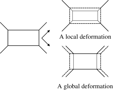
Figure 1: $(p,q)$ web description of the vanishing $\mathbb{P}^{1}\times\mathbb{P}^{1}$ geometry as in [17]. The two possible deformations are shown as “global” and “local”.

Toric Calabi-Yau’s can be seen as $T^{3}$ fibrations on a $3$-real dimensional base. The $(p,q)$ diagram describes the degeneration locus of this fibration: along the lines a $T^{2}$ is shrinking to zero size, and at the cubic vertices the full $T^{3}$ is vanishing.

The two parameters $a$ and $b$ in (3.1) correspond to the volumes of the two $\mathbb{P}^{1}$ in the compact $4$-cycle. More precisely, $b$ is related to the product of the volumes of the two $\mathbb{P}^{1}$’s, while $a$ is related to the difference between their areas. In figure 1 the finite segment are $\mathbb{P}^{1}$’s, and the rectangle describes the $4$-cycle $\mathbb{P}^{1}\times\mathbb{P}^{1}$.

From the metric (3.1) it is easy to see that, asymptotically at large radius, the $a$ parameter deforms the metric at order $1/r^{2}$, while the $b$ deformation only at order $1/r^{6}$. We can qualitatively interpret this fact simply looking at the $(p,q)$-web diagram: the $a$ deformation is changing the position of the branes at infinity (so it is a global deformation), while the the $b$ deformation does not, so it is a local deformation. In general, global deformations correspond to blowing up a $2$-cycle, and local deformations correspond to blowing up $4$-cycles.

In the case of vanishing $b$-deformation, the metric is a $\mathbb{Z}_{2}$ orbifold of the resolved conifold, given by (3.1) with $b=0$ and the period of $\psi$ taken to be $4\pi$. Notice also that (3.1) at $a=b=0$ is a special example of the $\mathcal{Y}^{p,q}$ metrics, specifically it is $\mathcal{Y}^{2,0}$. Equation (3.1) gives the most general Kähler Ricci-flat deformation of the conical metric $\mathcal{Y}^{2,0}$. Notice that the supergravity solution associated to $\mathcal{Y}^{2,0}$ has also additional moduli. For instance there is a moduli space of dual superconformal field theories (corresponding to $a=b=0$) of complex dimension $5$ [33], associated to changing the couplings of the theory. It is clear that these deformations are present also for $a$ and $b$ nonzero. It would be nice to investigate these more general theories.

3.1 Limit to Eguchi-Hanson

We now want to show that a double-scaling limit of (3.1) leads to the well-known Eguchi-Hanson metric. This is expected by looking at the toric description: sending the area of the rectangle in figure 1 to infinity while keeping fixed the size of one of the edges, one gets a $(p,q)$-web with two parallel semi-infinite legs, which is the space $\mathbb{C}\times\mathbb{C}^{2}/\mathbb{Z}_{2}$.

More precisely, sending the parameters $a$ and $b$ to infinity, we will recover the space $\mathbb{C}\times ALE$, where $ALE$ in this case is the total space of the line bundle ${\cal O}(-2)\rightarrow\mathbb{P}^{1}$ (it can also be seen as the Kähler Ricci-flat resolution of $\mathbb{C}^{2}/\mathbb{Z}_{2}$). We take the limit $(a,b)\rightarrow\infty$ with

$$c^{4}=\frac{4b^{6}}{81a^{2}}$$ (3.3)

fixed. In other words we focus on region of the geometry where $r\ll a,b$ but $r$ is of the same order as $c$. In this limit $\kappa(r)$ becomes

$$\kappa(r)=\frac{\frac{r^{2}}{a^{2}}+9-\frac{81c^{4}}{4r^{4}}}{\frac{r^{2}}{a^{2}}+6}\rightarrow\frac{3}{2}(1-\frac{9c^{4}}{4r^{4}}).$$ (3.4)

Let us now consider the term in 3.1 proportional to $(r^{2}+a^{2})$. In order to find a finite limit we rescale the coordinates $\theta_{2}$ and $\phi_{2}$ by a factor of $a$: $\tilde{\theta}=\frac{\theta_{2}}{a}$, $\tilde{\phi}=\frac{\phi_{2}}{a}$,

$$(r^{2}+a^{2})(d\theta_{2}^{2}+\sin^{2}\theta_{2}d\phi_{2}^{2})\rightarrow d\tilde{\theta}^{2}+\tilde{\theta}^{2}d\tilde{\phi}^{2}=d\textrm{x}^{2}_{2}.$$ (3.5)

We thus get the flat metric on $\mathbb{C}$, as expected from the fact that we are simply zooming in on a point of a smooth $2$-sphere. The piece in (3.1) proportional to $\kappa(r)$, keeping track of the rescaling of $\phi_{2}$ becomes

$$d\psi+\cos\theta_{1}d\phi_{1}+\cos\theta_{2}d\phi_{2}\rightarrow d\psi+\cos\theta_{1}d\phi_{1}.$$ (3.6)

At the end we see that the metric decomposes in one on $\mathbb{C}$ (3.5) and a remaining non-compact $4$-manifold: rescaling $R=r\sqrt{2/3}$

$$ds^{2}=\frac{dR^{2}}{1-\frac{c^{4}}{R^{4}}}+\frac{1}{4}(1-\frac{c^{4}}{R^{4}})R^{2}(d\psi+\cos\theta_{1}d\phi_{1})^{2}+\frac{1}{4}R^{2}(d\theta_{1}^{2}+\sin^{2}\theta_{1}d\phi_{1}^{2})+d\textrm{x}^{2}_{2}.$$ (3.7)

This is precisely the well-known Eguchi-Hanson metric. From a three dimensional point of view the limit space has isometries $SU(2)\times U(1)\times(\mathbb{R}^{2}\times SO(2))$.

3.2 The field theory dual

In this section we discuss the gauge theory living on $N$ D3 branes probing the local $\mathbb{P}^{1}\times\mathbb{P}^{1}$. The quiver diagram is well known: it has $4$ nodes and is reproduced in figure 1. The superpotential is readily obtained by imposing $SU(2)\times SU(2)$ invariance or by orbifolding the conifold field theory:

$$\mathcal{W}=\lambda tr\left(A_{\alpha}B_{\dot{\alpha}}C_{\beta}D_{\dot{\beta}}\right)\varepsilon^{\alpha\,\beta}\varepsilon^{\dot{\alpha}\,\dot{\beta}}.$$ (3.8)

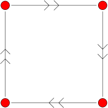
Figure 2: Quiver diagram for D3 branes probing the local $\mathbb{P}^{1}\times\mathbb{P}^{1}$ singularity.

We are interested in the moduli space of vacua of this field theory, which we obtain by analyzing $\mathcal{F}$ and $\mathcal{D}$ term relations on the fundamental fields of the theory. The full moduli space of the theory has complex dimension $3N$. $3(N-1)$ flat directions correspond to motion of the $N$ D3 branes in the Calabi-Yau. These are what we call “mesonic flat directions.” The remaining $3$ flat directions will be seen to be associated to the deformations of the geometry or to turning on $B$-fields. These can be called “non-mesonic” vevs. We will make use of the terminology of Fayet-Ilioupoulos parameters in order to describe the non-mesonic directions, even if this is not completely correct.

For our purposes it is enough to consider the case that the $N\times N$ matrices $A_{\alpha},B_{\dot{\alpha}},C_{\beta},D_{\dot{\beta}}$ commute. For the moment we also assume that all these $8$ complex matrices are proportional to the identity, corresponding to keeping the $N$ D3 branes coincident. It is easy to see that the $\mathcal{F}$ terms are solved if and only if

$$A_{\alpha} \propto C_{\alpha},$$ (3.9)

$$B_{\dot{\alpha}} \propto D_{\dot{\alpha}}\,,$$ (3.10)

which is equivalent to

$$A_{\alpha}=A\,e^{i\theta_{A}}\,n_{\alpha} C_{\alpha}=C\,e^{i\theta_{C}}\,n_{\alpha}$$ (3.11)

$$B_{\dot{\alpha}}=B\,e^{i\theta_{B}}\,m_{\dot{\alpha}} D_{\dot{\alpha}}=D\,e^{i\theta_{D}}\,m_{\dot{\alpha}}\,,$$ (3.12)

where $A,B,C,D$ are $4$ positive real numbers, the $\theta$’s are phases, $n_{\alpha}$ is parameterizing a $\mathbb{P}^{1}$ of unit radius and $m_{\dot{\alpha}}$ is parameterizing another $\mathbb{P}^{1}$ of unit radius. We already see the emergence of the geometry ($\mathbb{P}^{1}\times\mathbb{P}^{1}$). We now quotient by the gauge groups. These act by shifting the phases $\theta$. Using this freedom all the phases can be taken to be equal to $\psi$. $\mathcal{D}$ term relations read

$$A^{2}-B^{2}=t_{1},$$

$$B^{2}-C^{2}=t_{2},$$ (3.13)

$$C^{2}-D^{2}=t_{3},$$

$$D^{2}-A^{2}=t_{4},$$

where $t_{i}$ are the $4$ Fayet-Iliopoulos terms, that satisfy $t_{1}+t_{2}+t_{3}+t_{4}=0$, since in the sum of the $4$ previous relations the l.h.s. vanishes identically. This can also be seen by noticing that the diagonal $U(1)$ inside $U(N)^{4}$ is decoupled, since all fields are uncharged under it.

Notice that the solutions of eqs (3.2) are parameterized by a positive real line, and that the “smallest” possible vev is obtained when at least one of $A,B,C,D$ vanishes. Giving vev where one of these vanishes correspond to keeping the D3 branes at the smallest possible radius ($r=b$), and mesonic chiral operators are not taking vevs. If all the $A,B,C,D$ are non-vanishing, then also mesonic operators are taking vevs; this corresponds to moving the branes outside the resolved cycle.

We thus see that the mesonic moduli space of vacua is parameterized by $6$ real coordinates: $n_{\alpha}$, $m_{\dot{\alpha}}$, $\psi$ and one “radial” direction coming from $A,B,C,D$. It is simple to match these coordinates with the coordinates $(\theta_{1},\phi_{1})$, $(\theta_{2},\phi_{2})$, $\psi$, $r$.

We are now interested in an explicit map between the FI parameters $t_{i}$ in the gauge theory and the deformation parameters $a$ and $b$ in the geometry. Clearly the “conical” geometry $a=b=0$ corresponds to vanishing FI parameters, i.e. to conformal invariance.

3.3 The global deformation

Turning on only the global “$a$ deformation,” the space is the $\mathbb{Z}_{2}$ orbifold of the resolved conifold, so also in the field theory, we just have to “orbifold” the analysis of [11]. The final result is

$$t_{1}=-t_{2}=t_{3}=-t_{4}\propto a^{2}>0$$ (3.14)

Let us check this claim directly. Eqs. (3.2) in this case admit a “minimal” solution with

$$A=C=a_{f}\,,\;\;\;\;\;\;B=D=0$$ (3.15)

We thus see that the FI (3.14) are giving finite volume to the $\mathbb{P}^{1}$ parameterized by the $n_{\alpha}$, in accordance with the metric (3.1). At energies below the scale $t$, some fields are eaten by the Higgs mechanism and the field theory reduces in the infrared to a different field theory. The $U(N)$ gauge symmetries associated to node $1$ and $4$ are broken into a diagonal $U(N)$, because of the vev taken by $A$. Similar is the case for nodes $2$ and $3$. The infrared gauge symmetry is thus $U(N)\times U(N)$.

Let us assume that $A_{1}=C_{1}$ are the fields taking the vev $a_{f}$, that combine with the broken $U(N)\times U(N)$ gauge fields into massive gauge bosons. This assumption corresponds to putting the D3 branes at the “north-pole” of the blown-up $\mathbb{P}^{1}$ (of course any other point would lead to the same discussion, by $SU(2)$ symmetry). From the geometry, it is clear that the $a\rightarrow\infty$ limit, focusing on this point, is given by $\mathbb{C}\times\mathbb{C}^{2}/\mathbb{Z}_{2}$.

The IR quiver has only $6$ chiral fields. $A_{2}$ and $C_{2}$ transform as adjoint fields and the other $4$ fields as bifundamentals. Because of the $\varepsilon^{\alpha\beta}$ in the superpotential (3.8), we see that no massive terms in the superpotential are generated. All the superpotential terms are cubic and proportional to $\lambda\,\alpha_{f}$:

$$\mathcal{W}_{IR}=a_{f}\,\lambda\;tr\left(A_{2}B_{\dot{\alpha}}D_{\dot{\beta}}-B_{\dot{\alpha}}C_{2}D_{\dot{\beta}}\right)\varepsilon^{\dot{\alpha}\dot{\beta}}$$ (3.16)

This is precisely the matter content and superpotential corresponding the $\mathcal{N}=2$ field theory living at $\mathbb{C}\times\mathbb{C}^{2}/\mathbb{Z}_{2}$.

Let us end this paragraph studying the baryonic current as for the almost identical case of the conifold [11]:

$$\mathcal{K}_{B}=A_{\alpha}\bar{A}^{\alpha}-B_{\dot{\alpha}}\bar{B}^{\dot{\alpha}}+C_{\alpha}\bar{C}^{\alpha}-D_{\dot{\alpha}}\bar{D}^{\dot{\alpha}}.$$ (3.17)

We see that

$$<\mathcal{K}_{B}>\propto a^{2}.$$ (3.18)

This is precisely the dimension $2$ operator corresponding to the harmonic turned on at first order in the geometry, which at large $r$ undergoes corrections of order $1/r^{2}$. This order parameter has protected dimension since it is a conserved multiplet. The harmonic has its origin in the so called Betti multiplets, and was identified (for the very similar case of the conifold) in [31].

3.3.1 Global deformations from the metric: resolved conifold

The analysis presented in the previous subsections is nothing but an extension of the description of the small resolution of the conifold. Let us briefly recall what the precise picture is as presented by Klebanov and Witten in [11]. They argued that the natural gauge theory order parameter would be the lowest component of the baryonic supercurrent:

$${\cal U}={\rm Tr}(A_{i}\bar{A}_{i}-\bar{B}_{j}B_{j}).$$ (3.19)

${\cal U}$ has dimension two. A detailed analysis of this operator including its origin in the Betti multiplet is given in [31]. Given the explicit solution of D3 branes on the resolved conifold, we can quantitatively verify this claim. Namely, the supergravity solution in question is of the form (2.1) with [32]:

$$ds_{6}^{2} = \kappa(r)^{-1}dr^{2}+\kappa\,r^{2}e_{\psi}^{2}+r^{2}(e_{\theta_{1}}^{2}+e_{\phi_{1}}^{2})+(r^{2}+6a^{2})(e_{\theta_{1}}^{2}+e_{\phi_{1}}^{2}),$$

$$h = \frac{2L^{4}}{9a^{2}r^{2}}-\frac{2L^{4}}{81a^{4}}\ln\left(1+\frac{9a^{2}}{r^{2}}\right),\qquad\kappa=\frac{r^{2}+9a^{2}}{r^{2}+6a^{2}}.$$ (3.20)

The linearization of the solution can be written as:

$$ds^{2} = \frac{r^{2}}{L^{2}}dx_{\mu}dx^{\mu}+\frac{L^{2}}{r^{2}}dr^{2}+L^{2}ds^{2}(T^{1,1})$$ (3.21)

$$+ \frac{3a^{2}}{L^{2}}dx_{\mu}dx_{\mu}-\frac{6L^{2}a^{2}}{r^{4}}dr^{2}-\frac{3L^{2}a^{2}}{r^{2}}ds^{2}(X_{4})$$

$$+ \frac{36L^{2}a^{4}}{r^{4}}(d\psi+\sigma)^{2}+\ldots$$

In the first line, we have simply $AdS_{5}\times T^{1,1}$. From the second line we read that the solution corresponds to give a vacuum expectation value to a dimension two operator. One naturally has

$$<{\cal U}>\approx a^{2}.$$ (3.22)

The description above can be understood from the quiver gauge theory point of view. A convenient way to describe the small resolution of the conifold is in terms of four complex numbers satisfying the real constraint [11]

$$|a_{1}|^{2}+|a_{2}|^{2}-|b_{1}|^{2}-|b_{2}|^{2}=t,$$ (3.23)

where t is the area of the $P^{1}$, and then one takes the quotient by a $U(1)$ action. This is usually said as a gauged linear sigma model with $4$ fields, a $U(1)$ gauge group, where the charges of the fields are $(1,1,-1,-1)$. The above relation makes it clear that from the four dimensional quiver gauge theory point of view one is introducing a Fayet-Iliopoulos parameter.

3.4 General geometric deformation

We are left with other two FI parameters, and one other geometric deformation, that we called $b$. In the field theory there are two parameters, instead of one, because the field theory sees the full stringy moduli space, and the latter also includes a $B$-field that can be turned on.

Instead of talking in terms of FI parameters, we exhibit a possible solution on the moduli space of vacua of the gauge theory which corresponds to turning on both the $a$ and $b$ deformation. Consider giving vevs of the form

$$<A_{\alpha}> = \delta_{1\alpha}\,(a_{f}+b_{f})$$ (3.24)

$$<B_{\dot{\alpha}}> = \delta_{1\dot{\alpha}}\,\sqrt{2}b_{f}$$ (3.25)

$$<C_{\alpha}> = \delta_{1\alpha}\,(a_{f}-b_{f})$$ (3.26)

$$<D_{\dot{\alpha}}> = 0$$ (3.27)

Notice that the vev of the baryonic current is proportional to $a_{f}^{2}$ and does not depend on $b_{f}$. At energies greater than both $a_{f}$ and $b_{f}$ we have the UV conformal field theory with gauge symmetry $U(N)^{4}$. At energies $E$ such that $b_{f}<E<a_{f}$, we have the $\mathcal{N}=2$ field theory discussed above. Now, however, one bifundamental field, $B_{\dot{1}}$ is taking a vev $\sqrt{2}b_{f}$.

At energies $E<b_{f}$ the field theory is Higgsed to a $U(N)$ field theory with $5$ adjoints: $A_{2},C_{2},B_{\dot{2}},D_{\dot{1}},D_{\dot{2}}$. The superpotential

$$W=\lambda\;tr\left((a_{f}-b_{f})b_{f}A_{2}D_{2}-(a_{f}-b_{f})A_{2}B_{2}D_{1}+(a_{f}+b_{f})B_{2}C_{2}D_{1}-(a_{f}+b_{f})b_{f}C_{2}D_{2}\right)$$ (3.28)

contains mass terms for the fields $D_{2}$ and $(a_{f}-b_{f})A_{2}-(a_{f}+b_{f})C_{2}$; integrating these out, one finds the $\mathcal{N}=4$ SYM.

The conclusion is that the vevs (3.24) are in correspondence with the two geometric deformations discussed in the previous paragraph.

Comments on smearing of the D3 branes

For the gauge theory discussed above (all the D3 branes coincident and localized), the SUGRA metric including the gravitational backreaction of the D3 branes would break the $SU(2)\times SU(2)$ symmetry of rotations of the $n_{\alpha}$ $\mathbb{P}^{1}$, and for instance the warp factor would not be of the form (2.9). Putting instead a uniform distribution of D3 branes on the blown up $\mathbb{P}^{1}\times\mathbb{P}^{1}$, one can find a nice explicit supergravity solution, which is expected to be dual to the non-conformal gauge theory living on this distribution of D3 branes. In this case the solution is written in term of the Calabi-Yau metric as in (2.1) and the warp factor is like (2.9), depending only on $r$.

One general lesson from this discussion is that at order $1/r^{2}$ the corrections to the conformal solutions correspond to blown up $2$-cycles. Keeping these “global” deformations fixed, the order $1/r^{4}$ deformation only sees the total number of D3 branes. We can instead expect that corrections coming from how we distribute the branes on the blown up $4$-cycle play an important role at higher orders, starting at $1/r^{6}$. This should be analogous to the Coulomb branch solutions for $\mathcal{N}=4$ SYM [11].

3.5 Toric description of the blow up

Let us describe the process of the blowing-up from the point of view of toric geometry.

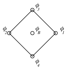
Figure 3: Toric description of the four-cycle in the orbifolded conifold.

The toric data before the blow up consist of four points on the outer square in figure 3. In the language of two-dimensional gauged linear sigma model, we introduce chiral superfields $\phi_{1,2,3,4}$ for each of the toric datum, and we introduce a vector multiplet $V_{1}$ to kill extra degrees of freedom. The toric data and the charge assignment is tabulated in the left hand side of table 1.

$$\begin{array}[]{c|cccc}&\phi_{1}&\phi_{2}&\phi_{3}&\phi_{4}\\ \hline\cr&1&1&1&1\\ &1&-1&0&0\\ &0&0&1&-1\\ V_{1}&1&1&-1&-1\end{array}\Longrightarrow\begin{array}[]{c|ccccc}&\phi_{1}&\phi_{2}&\phi_{3}&\phi_{4}&\phi_{B}\\ \hline\cr&1&1&1&1&1\\ &1&-1&0&0&0\\ &0&0&1&-1&0\\ V_{1}&1&1&-1&-1&0\\ V_{2}&1&1&1&1&-4\end{array}$$

Table 1: The charge assignments

Thus the toric manifold is described by the equations

$$|\phi_{1}|^{2}+|\phi_{2}|^{2}-|\phi_{3}|^{2}-|\phi_{4}|^{2}=0$$ (3.29)

divided by the identification

$$(\phi_{1},\phi_{2},\phi_{3},\phi_{4})\sim(e^{i\theta}\phi_{1},e^{i\theta}\phi_{2},e^{-i\theta}\phi_{3},e^{-i\theta}\phi_{4}).$$ (3.30)

This is precisely the cone over orbifolded $T^{1,1}$.

In order to blow up the four-cycle corresponding to the internal point in figure 3, we add a corresponding chiral superfield $\phi_{B}$ and another vector superfield as in the right hand side of the table 1. Now the equations describing the toric manifold are

$$|\phi_{1}|^{2}+|\phi_{2}|^{2}-|\phi_{3}|^{2}-|\phi_{4}|^{2} = 0$$ (3.31)

$$|\phi_{1}|^{2}+|\phi_{2}|^{2}+|\phi_{3}|^{2}+|\phi_{4}|^{2}-4|\phi_{B}|^{2} = t$$ (3.32)

under the identification

$$(\phi_{1},\phi_{2},\phi_{3},\phi_{4},\phi_{B}) \sim (e^{i\theta}\phi_{1},e^{i\theta}\phi_{2},e^{-i\theta}\phi_{3},e^{-i\theta}\phi_{4},\phi_{B}),$$ (3.33)

$$(\phi_{1},\phi_{2},\phi_{3},\phi_{4},\phi_{B}) \sim (e^{i\theta}\phi_{1},e^{i\theta}\phi_{2},e^{i\theta}\phi_{3},e^{i\theta}\phi_{4},e^{-4i\theta}\phi_{B}).$$ (3.34)

where $t\geq 0$ is the Fayet-Iliopoulos term for the vector multiplet $V_{2}$, which controls the size of the blown-up four-cycle.

Let us explicitly see that we have $\mathbb{P}^{1}\times\mathbb{P}^{1}$ of non-zero size. Let us slice the manifold at constant $|\phi_{B}|^{2}=c$. If $c>0$, we can fix the second identification (3.34) by setting $\phi_{B}$ at a positive real number. The rest of the equation is

$$|\phi_{1}|^{2}+|\phi_{2}|^{2}=|\phi_{3}|^{2}+|\phi_{4}|^{2}=t/2+2c,$$ (3.35)

which is a product of two $S^{3}$ of the same size. We get $T^{1,1}/Z_{2}$ after dividing by the identification (3.33). When $c=0$, we can no longer fix (3.34) using $\phi_{B}$. Thus, we need to divide (3.35) by (3.33) and (3.34), which yields $\mathbb{P}^{1}\times\mathbb{P}^{1}$ of radius $\sqrt{t/2}$. This is precisely the local deformation discussed in the previous subsections.

We can also introduce the Fayet-Iliopoulos term to (3.31). One can easily see that it changes the relative size of two $P_{1}$. It is the global deformation in our parlance.

3.6 Comments on the 4-cycle deformation of the Klebanov-Strassler solution

In this section we have seen that a $\mathbb{Z}_{2}$ orbifold of the conifold admits $3$ deformations associated to giving vev to fundamental fields (these are $3$ non mesonic direction in the field theory moduli space). One deformation corresponds to a blown up $2$ cycle, one to a blown up $4$ cycle, one to a $B$ field. In the case of the conifold only one deformation is present, the so called resolved conifold, corresponding to a blown up $2$ cycle, which can be called the “baryonic flat direction.”

We know that the resolution of the conifold plays an important role also after the addition of fractional branes. The moduli space of vacua (for certain values of the number of fractional branes) contains a baryonic branch, which comes from the “baryonic flat direction” discussed above. For a thorough analysis see [26]. The Klebanov-Strassler [21] solution corresponds to a field theory sitting on this baryonic branch at the special point $a=0$ (in our notation).

Very interestingly, there is indeed a generalization of the Klebanov-Strassler background corresponding to this “ Kähler” modulus, this is the so called baryonic branch solution, found for small deformation parameters in [27] and at all orders, using $SU(3)$ structures, in [29].

From our analysis it is natural to expect that also for the local $\mathbb{P}^{1}\times\mathbb{P}^{1}$ geometry, after adding fractional branes, there is a non-mesonic branch. It is very simple to obtain the baryonic branch solution with fractional branes for our case: we just have to take the solution of [29] but declare the periodicity of the angle $\psi$ to be $2\pi$ instead of $4\pi$.

The point is that this $\mathbb{Z}_{2}$ orbifold of the baryonic branch also admits a deformation corresponding to the $b$ parameter. We think it would be very interesting to study this problem. Notice that the full solution should be captured by functions of only one variables (as in [29]), since the $b$ deformation is not breaking any further continuous symmetry. As a first step it would be interesting to identify the massless mode that should appear in the twisted sector of the orbifold. It would also be important to improve the field theory analysis along the lines of [26].

4 Blowing up $4$-cycles: the general case

4.1 Deformations and Operators

Let us consider various aspects of the general case. Given a resolved local Calabi-Yau, there a two types of Kähler deformations. One corresponds to changing the size of a $\mathbb{P}^{1}$ as described by the parameter $a$, the other to changing the size of a four cycle described by the $b$-parameter. For toric CY there is a dual description in terms of a $(p,q)$-web. The $a$-deformation changes the position of the branes at infinity, while the $b$-deformation is a “local” deformation, it only change the sizes of the internal faces, without moving the external branes. In this sense the $a$-deformation is heavy and requires a lot of energy, while the local $b$-deformation does not require a lot of energy. For a complicated CY there are many independent $a$- and $b$-deformations. The number of $a$-deformations is the number of external legs (denoted by $d$ ) minus 3. The number of $b$-deformations is the number of internal points in the toric diagram (denoted by $I$ ), which will be discussed further in section 4.3. The universal $b$-deformation we described in section 2 is a particular example of this class.

From the examples considered in this paper it is natural to conjecture that the change of the metric at large radius is always of the type $1/r^{2}$ for $a$-deformations, while it is $1/r^{6}$ for $b$-deformations.

The $a$-deformation in the field theory has as order parameter the corresponding (scalar superpartner of the) baryonic current, which has always dimension $2$, matching with the $1/r^{2}$ correction to the metric. The number of global deformation is always given by the number of external legs in the $(p,q)$ diagram minus $3$.

For the $b$-deformation we expect to find as many dimension six operators in the field theory as four cycles in the geometry which coincide with the number of internal points in the toric diagram. The total number of gauge groups is always given by twice the area of the toric diagram. The area, by Pick’s theorem, is expressible in terms of the number of external points $d$ and the number of internal points $I$. Concluding, the number of gauge groups is

$$\#\textrm{gauge-groups}=1+(d-3)+2I.$$ (4.1)

Now, the number of formal FI parameters that can be turned on is the number of gauge groups minus $1$ (recall no field is charged under the diagonal $U(1)$). $d-3$ such FI parameters are associated to the $d-3$ baryonic symmetries. Among the other $2I$ FI parameters, $I$ are associated to the $I$ $4$-cycles that can be blown up. The remaining $I$ FI parameters have thus to be associated to $B$-fields that can be turned on in the supergravity solution.

We have thus matched the number of the three possible deformations (global, local and $B$-fields) with the formal FI parameters in the field theory.

This matching strongly suggests that the operators of dimension six turned on by the local deformation are associated with the gauge groups in the quiver. We thus propose that these operators are roughly of the form:

$$\mathcal{O}_{i}=\sum_{g}c_{i,g}\mathcal{W}_{g}\bar{\mathcal{W}_{g}}$$ (4.2)

where the sum is over the gauge groups in the quiver.

Notice that similar operators are present in the supergravity background of $T^{1,1}$ [30, 31], and are also turned on in the baryonic branch of the Klebanov-Strassler solution [29].

4.2 More on $a$-deformation

Indeed, we can check that the dimension of operators corresponding to the $a$-deformations are two, and there are $d-3$ of them for the compactification on the toric Sasaki-Einstein $X$. The argument is a generalization of one given in [11]. The original metric on the cone is

$$ds^{2}=dr^{2}+r^{2}ds_{X}^{2}.$$ (4.3)

Let us blow up some two-cycles and four-cycles at the tip of the cone (see figure 4), and let us denote the Kähler form before and after the blowup by $J$ and $J+\delta J$, respectively. Note that $J$ behaves as

$$J\sim r^{2}$$ (4.4)

when $r\to\infty$.

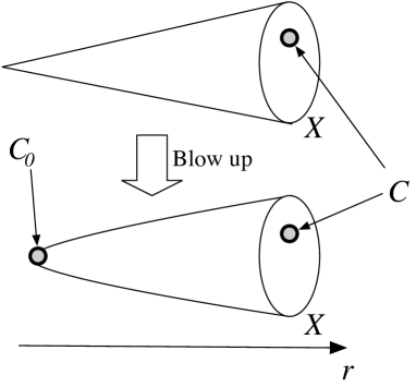
Figure 4: $a$-type deformation

Suppose that there is a supersymmetric two-cycle $C_{0}$ at the tip which comes from a two-cycle $C$ in the Sasaki-Einstein $X$, and let us blow-up so that $C_{0}$ has area $t$. Then,

$$t=\int_{C_{0}}\sqrt{g}=\int_{C_{0}}J+\delta J,$$ (4.5)

because the supersymmetric cycle should be calibrated with respect to the Kähler form. Now, since $C_{0}$ and $C$ are in the same homology class, we have

$$t=\int_{C}J+\delta J.$$ (4.6)

Since we assumed that $C$ is a nontrivial homology class in $H_{2}(X)$, we can take $C$ at arbitrarily large $r$. It means that $\delta J$ has the behavior $\sim r^{0}$ under $r\to\infty$. Compared to (4.4), it is a $1/r^{2}$ type deformation, which corresponds to a dimension two operator in the dual CFT. Thus we see that there is an $a$-type deformation for each homology class in $H_{2}(X)$. From Poincaré duality in $X$, $H_{2}(X)$ has the same dimension $d-3$ as $H_{3}(X)$, which corresponds to the baryonic symmetries.

From the viewpoint of the SCFT, the superconformal algebra fixes the dimension of the scalar operator in the superconformal multiplet of a conserved flavor current so that it has dimension two. For the SCFT dual to the type IIB theory on $AdS_{5}\times X$, there is $d-1$ flavor symmetry. $d-3$ of them are the so-called baryonic symmetries, and the modes we found for each of the homology class in $H_{2}(X)$ are the dual manifestation in the gravity side. It would be interesting to find the remaining two modes. This description allows us to canonically identify corresponding operator as the lowest component of the supercurrent that generates the baryonic symmetry.

4.3 Global issues

Next, let us discuss the issues concerning the global topology of the $b$-deformation. Recall that in section 2 we obtained that near the point $r\approx b$, the metric takes the form:

$$ds^{2}\approx du^{2}+9u^{2}(d\psi+\sigma)^{2}+b^{2}ds_{4}^{2}.$$ (4.7)

In order to avoid conical singularities, we require the periodicity of $3\psi$ to be $2\pi$. In the case of the conifold, what we call $3\psi$ here, has period $4\pi$. In order to avoid conical singularities we must, therefore, introduce a $\mathbb{Z}_{2}$ orbifold ending up with $T^{1,1}/\mathbb{Z}_{2}$. Similarly, for $S^{5}$ written as a $U(1)$ bundle over $\mathbb{C}\mathbb{P}^{2}$, we have to impose a $\mathbb{Z}_{3}$ orbifold in order to avoid conical singularities and we are left with $S^{5}/\mathbb{Z}_{3}$. For the general $Y^{p,q}$ and $L^{p,q,r}$, in the quasi-regular case a specific quotient is required.

There is a beautiful picture of the above situation that arises from the toric diagram of the original Calabi-Yau singularity. As can be seen from the metric in (4.7) at the origin of space $r=b$, there is a 4-cycle with finite volume proportional to $b$. We can try to view this 4-cycle more algebraically. A particularly useful tool is the toric diagram. Let us consider the example of the conifold. Recall that 4-cycles that can be blown up appear in the toric diagram as internal points. Therefore, we expect to relate the quotient to the generation of internal points in the toric diagram. Let us take the example of the conifold. The toric diagram of the conifold is simply a square with no internal points. After the quotient by $\mathbb{Z}_{2}$, we have precisely an internal point which we show in blue in figure 5.

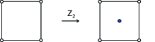
Figure 5: A four cycle in the orbifolded conifold.

We think of the orbifold in the sense of

$$\mathbb{Z}^{2}\subseteq L\subseteq\left(\frac{1}{2}\mathbb{Z}\right)^{2},$$ (4.8)

where

$$L:=\{(n_{1},n_{2}):\,\,\sum n_{i}\in\mathbb{Z}\}.$$ (4.9)

Clearly the point $(\frac{1}{2},\frac{1}{2})$ belongs to the lattice $L$ and corresponds to the point in the middle in figure 5. A concrete process of blowing up a four-cycle corresponding to an internal point is already presented in section 3.5.

For $\mathbb{C}^{3}$, after a $\mathbb{Z}_{3}$ orbifold, we see that the toric diagram contains an internal point, also shown in blue in figure 6.

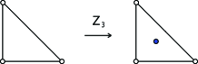
Figure 6: A four cycle in the orbifolded $\mathbb{C}^{3}$.

The situation for the $\mathbb{Z}_{3}$ orbifold of $\mathbb{C}^{3}$ is conceptually similar although technically slightly more complicated. The off shot is that the quotient indeed generates an internal point. Basically, taking the quotient $\mathbb{C}^{3}/\mathbb{Z}_{3}$ adds a point with coordinates $\frac{1}{3}(1,1,1)$ in a lattice where the original triangle had coordinates $(1,0,0),(0,1,0)$ and $(0,0,1)$. This point corresponds precisely to acting with a cube root of one contained in $(\mathbb{C}^{*})^{3}$. The internal point algebraically describes a blow up mode which is geometrically captured in equation 4.7.

The observation above can be extended to any of the internal points of the toric diagram. We follow the notation and language of [35]. Let us choose the basis of the $N$ lattice such that the toric data can be given as $k_{I}=(1,\vec{k}_{I})$. When the Sasaki-Einstein is regular, then the Reeb vector $R$ is the integral combination of the generator of $T^{3}$ defining the toric geometry. It means $R$ is on the $N$ lattice. Furthermore, it is guaranteed to be on the same plane in $N$ as the other toric data. Thus $R=(1,\vec{R})$ with integer entries.

Now add $R$ to the toric data $\{k_{1},k_{2},\ldots\}$ and consider the toric manifold $Z$ defined by these points. $Z$ is a blowup of the cone over $X$, and since all the toric data $R$ and $k_{I}$ lie on a plane, $Z$ is at least topologically Calabi-Yau. Let us recall that, in the gauged linear sigma model description, we introduce chiral superfields $x_{v}$ for each $v$ in the toric data and do the symplectic reduction. Thus for each vector $v$ in the toric data, we have a divisor $D_{v}$ defined by $x_{v}=0$ where the vector $v$ degenerates. We can now see that $Z$ has precisely the topology of the $b$-deformation of the cone over $X$.

4.4 Topological restriction of the $b$-deformation

Let us elaborate the discussion on the need for the orbifolding. First let us see, in order for the $b$-deformation to make sense, the Sasaki-Einstein manifold needs to be regular or quasi-regular. It can be argued in many ways. One way goes as follows: near $r\sim b$, the metric looks locally like (4.7). Fix $u=u_{0}$ small and nonzero. Then the $u=u_{0}$ surface is topologically the same as the original Sasaki-Einstein $X$. Suppose the base Kähler-Einstein manifold $Y$ exist globally. Forgetting the $\psi$ coordinate determines the map $p:X\to Y$. If two points $a$ and $b$ on $X$ are related by the action of $\partial_{\psi}$ then $p(a)=p(b)$. In the regular or quasi-regular case, a circle on $X$ projects to a point on $Y$. However in the irregular case, the action of the Reeb vector $\partial_{\psi}$ does not close and fills a $T^{2}$ or $T^{3}$. Thus $Y$ cannot be a four-dimensional manifold. For example, $Y^{p,q}$ is quasi-regular only when there is an integer $n$ such that $4p^{2}-3q^{2}=n^{2}$. In these cases, the $\psi$ direction closes with some periodicity $2\pi s/3$. Then we obtain a good $b$-deformation by orbifolding along the $\psi$ direction by $\mathbb{Z}_{s}$, although a small technical issue still remains, which is discussed further in appendix D.

The main point we would like to raise is the fact that although locally the $b$-deformation is allowed the mere presentation of a Sasaki-Einstein manifold in the form of (4.7) does not guarantee that the manifold exists globally. In fact, in several cases one needs to find appropriate alternative coordinate in which to demonstrate the existence of the SE manifold. However, it is clear that if the base manifold exist for $b=0$ it also exists for $b\neq 0$.

The result can also be expressed in the following way.

As we saw, the blow-up four-cycles are governed by the internal points on the diagram, where the point specifies which direction of $T^{3}$ is degenerating along the four-cycle. The Reeb vector $R$ also defines a point on the toric diagram, and when the universal deformation is possible, $R$ degenerates along the four-cycle. Thus, $R$ must be on the internal integral points in order to do the universal $b$-deformation. The orbit of the Reeb vector closes or not according to whether $R$ lies on a rational point or an irrational point. In the former case, we can take a suitable orbifold to make the vector to sit on an internal integral point, while in the latter there is no way to make it integral.

5 Fractional branes and $b$-deformation

Given a quiver diagram describing a conformal field theory, a simple way to upset the vanishing of the beta functions is by changing the rank of some of the gauge groups. In the supergravity side this operation corresponds to the introduction of fractional branes. This is a universal mechanism discussed in [20, 21, 25]. The addition of fractional branes generalizes to many of the six-dimensional metrics discussed here. That is, the ten-dimensional supergravity solution based on them accommodates fractional D3 branes. In this section we show that if a Calabi-Yau cone admits fractional D3 branes then its deformation by a parameter $b$ also admits fractional branes, where the fractional brane corresponds to D5 branes wrapping a two-cycle in the blown-up four-cycle.

The presence of fractional branes manifest itself in the gravity theory by the appearance of an imaginary self-dual 3-form flux $G_{3}$. For the cone over Sasaki-Einstein metrics we have that $M$ fractional branes are described by

$$G_{3}=M\left(\frac{dr}{r}+ie^{\psi}\right)\wedge\omega,$$ (5.1)

where $\omega$ is an appropriately chosen 2-form on the four dimensional base. Suppose such a construction of $G_{3}$ is allowed for a metric of the form

$$ds^{2}=dr^{2}+r^{2}(e^{\psi})^{2}+r^{2}ds_{4}^{2},$$ (5.2)

with $ds_{4}^{2}$ a Kähler-Einstein metric. Then, the $b$-deformed metric

$$ds^{2}=\kappa(r)^{-1}dr^{2}+{\kappa}r^{2}(e^{\psi})^{2}+r^{2}ds_{4}^{2},$$ (5.3)

where $\kappa=1-b^{6}/r^{6}$, also admits an imaginary self-dual 3-form flux. In other words, the $b$-deformation does not interfere with the property of the cone metric to admit both regular and fractional branes.

One can write an imaginary self-dual 3-form for the cone metric (5.2), if there exists an anti self dual $(1,1)$-form on the four dimensional base satisfying

$$d\omega = 0,$$

$$J\wedge\omega = 0,$$

$$*_{4}\omega = -\omega,$$ (5.4)

where $J$ is the Kähler form and $*_{4}$ is the Hodge dual taken with respect to the four dimensional metric. Then the relevant 3-form for $M$ fractional D3 branes is given precisely by (5.1). The relevant properties of (5.1) are:

$$dG_{3} = 0,$$

$${*}_{6}G_{3} = iG_{3}.$$ (5.5)

They can be verified using (5.4) as:

$$dG_{3} = M[-r^{-1}dr\wedge d\omega+ide^{\psi}\wedge\omega-ie^{\psi}\wedge d\omega]=0,$$

$${*}_{6}G_{3} = M[e^{\psi}\wedge*_{4}\omega-ir^{-1}dr\wedge*_{4}\omega]$$

$$= iM[r^{-1}dr\wedge\omega+ie^{\psi}\wedge\omega]$$

$$= iG_{3},$$

where in the first line we used that $de^{\psi}=2J$. For the $b$-deformed metric (5.3), we simply take

$$G_{3}=M\left(\frac{dr}{\kappa r}+ie^{\psi}\right)\wedge\omega.$$ (5.7)

Then proceeding along exactly similar lines, one finds that this 3-form satisfies the properties (5.5) for the metric (5.3). This construction has been used to obtain imaginary self-dual 3-form for certain cases, see for example [14, 15, 16, 21, 22, 23, 7, 32].

In a neighborhood of $r\sim b$, (5.7) can be rewritten as

$$G_{3}=M(\frac{du}{u}+ie^{\psi})\wedge\omega,$$ (5.8)

where $u$ is a variable introduced in (2.4). Take a two-cycle $C$ dual to $\omega$ on the blown-up four-cycle so that $\int_{C}\omega=0$. Let us take a small circle $c$ around the origin $u=0$ which winds around $\psi$ direction once. Then

$$\int_{c\times C}G_{3}=2\pi,$$ (5.9)

which means that the self-dual three-form field strength is sourced by the D5 brane wrapped on the two-cycle dual to $C$ and representing $\omega$. Thus, the fractional D3 brane is now realized as a D5 brane wrapping around the two-cycle.

6 Conclusion

In this paper we have studied a Kähler deformation of Calabi-Yau spaces that can be obtained as cones over Sasaki-Einstein spaces. This is a very large class of spaces that have been playing an important role in the AdS/CFT. We have described this deformation explicitly in terms of toric geometry and studied its field theory dual. We showed that this deformation corresponds to giving a vacuum expectation value to a scalar dimension six operator with vanishing $R$-charge and gave a suggestion for the the precise form of this operator. Interestingly, a probe string in these backgrounds signals area-law confinement (see appendix E for details). Thus, we provide a universal Kähler deformation that induces confinement in a large class of quiver gauge theories. We have also discussed some interesting relations with a better-studied Kähler deformation called the small resolution in the case of a $\mathbb{Z}_{2}$ orbifold of the conifold, the so-called local $\mathbb{P}^{1}\times\mathbb{P}^{1}$.

Some open questions remain. For example, we would like to improve our understanding of the Kähler deformation from the algebraic point of view. We did not find a fully satisfactory connection between the gauged linear sigma model analysis and the supergravity prediction. Analogously, we would like to understand better the role of the dimension six operators at the level of field theory, possibly directly in the quiver diagram. We hope to return to some of these questions in future work.

We argued that there are as many Kähler deformations corresponding to blowing up 4-cycles as internal points in the toric diagram. In this paper we have considered turning on only one of them. It would be interesting to understand the general case. Presumably, the general case corresponds to generalizations of the metric of equation (3.1) in the same way as the Gibbons-Hawking metric generalizes the Eguchi-Hanson metric. What is needed would be the Gibbons-Hawking metric with $U(1)\times U(1)$ isometries, i.e. when all the point-charges lie in a line. Similarly, it would be interested to consider the general case of Kähler deformations corresponding to blowing up 2-cycles.

Appendix A Ricci flatness

In this appendix, we explicitly show that the metric is Ricci flat. This fact was established very generally in [13], but we will use some of the intermediate results in the main text. In particular, arguments about supersymmetry rely on the explicit form of the spin connection.

$$ds^{2}=A^{2}(r)dr^{2}+B^{2}(r)(d\psi+\sigma)^{2}+C^{2}(r)ds_{4}^{2}$$ (A.1)

The one forms are

$${e}^{r} = A(r)dr$$

$${e}^{\psi} = B(r)(d\psi+\sigma)$$

$${e}^{i} = C(r){\hat{e}}_{i}\;\;\;\;(i=1..4)$$ (A.2)

They are chosen such that the metric is orthonormal. $d\sigma=2J$ and $J=\frac{1}{2}J_{ij}\hat{e}^{i}\wedge\hat{e}^{j}$. Superscript hat denotes the quantities with respect to four-dimensional base. The one forms are

$$d{e}^{r} = 0$$

$$d{e}^{\psi} = \frac{B^{\prime}}{AB}{{e}^{r}}\wedge{{e}^{\psi}}+\frac{B}{C^{2}}J_{ij}e^{i}\wedge e^{j}$$

$$d{e}^{i} = \frac{C^{\prime}}{AC}{{e}^{r}}\wedge{{e}^{i}}-C^{-1}{\hat{\omega}}{{}^{i}}_{jk}{e}^{k}\wedge{e}^{j}$$ (A.3)

Prime means derivative with respect to $r$. ${\hat{\omega}}{{}^{i}}_{j}={\hat{\omega}}{{}^{i}}_{jk}\hat{e}^{k}$. For $de^{a}=-\frac{1}{2}C{{}_{bc}}^{a}e^{b}\wedge e^{c}$, we get

$$C{{}_{ab}}^{r} = 0$$

$$C{{}_{r\psi}}^{\psi} = -\frac{B^{\prime}}{AB}$$

$$C{{}_{ij}}^{\psi} = -\frac{2B}{C^{2}}J_{ij}$$

$$C{{}_{ri}}^{i} = -\frac{C^{\prime}}{AC}$$

$$C{{}_{jk}}^{i} = -\frac{1}{C}{\hat{\omega}}{{}^{i}}_{jk}$$ (A.4)

Then the spin-coefficients are

$${\omega}_{r\psi} = -\frac{B^{\prime}}{AB}{e}^{\psi}$$

$${\omega}_{ri} = -\frac{C^{\prime}}{AC}{e}^{i}$$

$${\omega}_{\psi i} = \frac{B}{C^{2}}J_{ij}e^{j}$$

$${\omega}_{ij} = {\hat{\omega}}_{ij}-\frac{B}{C^{2}}J_{ij}{e}^{\psi}$$ (A.5)

This leads to Ricci two form components using ${\theta}_{ij}=dw_{ij}+w_{ik}\wedge w{{}^{k}}_{j}$ The indices are raised and lowered in this case by ${\delta}{{}^{i}}_{j}$.

$${\theta}_{r\psi} = -\frac{1}{AB}\left(\frac{B^{\prime}}{A}\right)^{\prime}{{e}^{r}}\wedge{{e}^{\psi}}-\frac{1}{AC^{3}}(B^{\prime}C-BC^{\prime})J_{ij}e^{i}\wedge e^{j}$$

$${\theta}_{ri} = -\frac{1}{AC}\left(\frac{C^{\prime}}{A}\right)^{\prime}{{e}^{r}}\wedge{{e}^{i}}+\frac{1}{AC^{3}}(B^{\prime}C-BC^{\prime})J_{ij}{e}^{j}\wedge{e}^{\psi}$$

$${\theta}_{\psi i} = \frac{1}{AC^{3}}(B^{\prime}C-BC^{\prime})J_{ij}e^{r}\wedge e^{j}+\left[\left(\frac{B}{C^{2}}\right)^{2}-\frac{B^{\prime}C^{\prime}}{A^{2}BC}\right]e^{\psi}\wedge e^{i}$$

$$+\frac{B}{C^{2}}(DJ_{ij})\wedge e^{j}$$

$${\theta}_{ij} = {\hat{\theta}}_{ij}-\frac{2}{AC^{3}}(B^{\prime}C-BC^{\prime})J_{ij}e^{r}\wedge e^{\psi}$$

$$-\left(\frac{B}{C^{2}}\right)^{2}(J_{ij}J_{kl}+J_{ik}J_{jl})e^{k}\wedge e^{l}-\left(\frac{C^{\prime}}{AC}\right)^{2}e^{i}\wedge e^{j}$$

$$-\frac{B}{C^{2}}(DJ_{ij})\wedge e^{\psi}$$

$$\textrm{where }DJ_{ij} = dJ_{ij}-J_{ik}{\hat{\omega}}{{}^{k}}_{j}+{\hat{\omega}}_{ik}J{{}^{k}}_{j}$$ (A.6)

Let us invoke here $DJ_{ij}=0$. Since ${\theta}{{}^{a}}_{b}=\frac{1}{2}R{{}^{a}}_{bcd}e^{c}\wedge e^{d}$, one can get

$$R_{r\psi r\psi}=-\frac{1}{AB}\left(\frac{B^{\prime}}{A}\right)^{\prime} R_{r\psi ij}=-\frac{2}{AC^{3}}(B^{\prime}C-BC^{\prime})J_{ij}$$

$$R_{riri}=-\frac{1}{AC}\left(\frac{C^{\prime}}{A}\right)^{\prime} R_{rij\psi}=\frac{1}{AC^{3}}(B^{\prime}C-BC^{\prime})J_{ij}$$

$$R_{\psi irj}=\frac{1}{AC^{3}}(B^{\prime}C-BC^{\prime})J_{ij} R_{\psi ii\psi}=\frac{B^{\prime}C^{\prime}}{A^{2}BC}-\left(\frac{B}{C^{2}}\right)^{2}$$

$$R_{ijkl}=C^{-2}{\hat{R}}_{ijkl}-\left(\frac{B}{C^{2}}\right)^{2}(2J_{ij}J_{kl}+J_{ik}J_{jl}-J_{il}J_{jk}) - \left(\frac{C^{\prime}}{AC}\right)^{2}({\delta}_{ik}{\delta}_{jl}-{\delta}_{il}{\delta}_{jk})$$

$$R_{ijr\psi}=-\frac{2}{AC^{3}}(B^{\prime}C-BC^{\prime})J_{ij}$$ (A.7)

This gives

$$R_{rr} = -\frac{1}{AB}\left(\frac{B^{\prime}}{A}\right)^{\prime}-\frac{4}{AC}\left(\frac{C^{\prime}}{A}\right)^{\prime}$$

$$R_{\psi\psi} = -\frac{1}{AB}\left(\frac{B^{\prime}}{A}\right)^{\prime}-\frac{4B^{\prime}C^{\prime}}{A^{2}BC}+4\left(\frac{B}{C^{2}}\right)^{2}$$

$$R_{ii}({\textrm{ no sum }}) = -\frac{1}{AC}\left(\frac{C^{\prime}}{A}\right)^{\prime}-\frac{B^{\prime}C^{\prime}}{A^{2}BC}+\left(\frac{B}{C^{2}}\right)^{2}+C^{-2}{\hat{R}}_{ii}+2\left(\frac{B}{C^{2}}\right)^{2}{\delta}_{ii}-3\left(\frac{C^{\prime}}{AC}\right)^{2}{\delta}_{ii}$$

$$R_{ij}\;\;(i\neq j) = C^{-2}{\hat{R}}_{ij}$$ (A.8)

For Einstein base, ${\hat{R}}_{ij}$ is proportional to metric. Since we are doing calculations in orthonormal frame, it vanishes for $i\neq j$. The Ricci flatness conditions are

$$-\frac{1}{4AB}\left(\frac{B^{\prime}}{A}\right)^{\prime}-\frac{1}{AC}\left(\frac{C^{\prime}}{A}\right)^{\prime}=0$$

$$-\frac{1}{4AB}\left(\frac{B^{\prime}}{A}\right)^{\prime}-\frac{B^{\prime}C^{\prime}}{A^{2}BC}+\left(\frac{B}{C^{2}}\right)^{2}=0$$

$$C^{-2}{\lambda}+\frac{1}{2AB}\left(\frac{B^{\prime}}{A}\right)^{\prime}+2\left(\frac{B}{C^{2}}\right)^{2}-3\left(\frac{C^{\prime}}{AC}\right)^{2} = 0$$ (A.9)

where $\hat{R}_{ij}={\lambda}\hat{g}_{ij}$ for the Einstein base. A general solution for these equations was obtained in [13]. The equations are easier to handle if one chooses $AB=c$ (a constant) in the beginning. The solution is

$$d\hat{s}^{2}=(1-r^{2})^{2}P(r)^{-1}dr^{2}+c^{2}(1-r^{2})^{-2}P(r)(d\psi+\sigma)^{2}+c(1-r^{2})ds_{4}^{2}$$ (A.10)

where, $P(r)$ is a polynomial in $r$. If one imposes the condition for the metric to be Kähler, then it takes the form

$$d\hat{s}^{2} = U^{-1}d{\rho}^{2}+U{\rho}^{2}(d\tau+\sigma)^{2}+{\rho}^{2}ds_{4}^{2}$$

$$U = \frac{\lambda}{6}+c_{0}{\rho}^{-6}$$ (A.11)

$c_{0}$ is a constant. If now one sets $\lambda=2(n+1)$, then

$$d\hat{s}^{2}=\left[1-\left(\frac{b}{\rho}\right)^{6}\right]^{-1}d{\rho}^{2}+\left[1-\left(\frac{b}{\rho}\right)^{6}\right]{\rho}^{2}(d\psi+\sigma)^{2}+{\rho}^{2}ds_{4}^{2}$$ (A.12)

So the b-deformed metric is the most general Calabi-Yau metric of type A.1.

Appendix B Supersymmetry

We will write down the integrability conditions for these metrics to be supersymmetric. We check here that deformation by b-parameter do not spoil supersymmetry. The integrability conditions $R_{abcd}{\Gamma}^{cd}\varepsilon=0$ written explicitly are

$$-\frac{1}{AB}\left(\frac{B^{\prime}}{A}\right)^{\prime}{\Gamma}^{r\psi}\varepsilon-\frac{2}{AC^{3}}(B^{\prime}C-BC^{\prime})J_{ij}{\Gamma}^{ij}\varepsilon=0$$

$$-\frac{1}{AC}\left(\frac{C^{\prime}}{A}\right)^{\prime}{\Gamma}^{ri}\varepsilon+\frac{1}{AC^{3}}(B^{\prime}C-BC^{\prime})J{{}^{i}}_{j}{\Gamma}^{j\psi}\varepsilon=0$$

$$\frac{1}{AC^{3}}(B^{\prime}C-BC^{\prime})J_{ij}{\Gamma}^{rj}\varepsilon+\left(\frac{B^{\prime}C^{\prime}}{A^{2}BC}-\frac{B^{2}}{C^{4}}\right){\Gamma}^{i\psi}\varepsilon=0$$

$$C^{-2}\hat{R}_{ijkl}{\Gamma}^{kl}\varepsilon-2\frac{B^{2}}{C^{4}}(J_{ij}J_{kl}+J_{ik}J_{jl}){\Gamma}^{kl}\varepsilon-2\left(\frac{C^{\prime}}{AC}\right)^{2}{\Gamma}^{ij}\varepsilon-\frac{2}{AC^{3}}(B^{\prime}C-BC^{\prime})J_{ij}{\Gamma}^{r\psi}\varepsilon=0$$

For the case of $A=1,B=C=r$, the only nontrivial equation is

$$\hat{R}_{ijkl}{\Gamma}^{kl}\varepsilon-2(J_{ij}J_{kl}+J_{ik}J_{jl}){\Gamma}^{kl}\varepsilon-2\Gamma_{ij}\varepsilon=0$$ (B.2)

For $A={\kappa}^{-1/2},B=\kappa^{1/2}r,C=r$ with $\kappa=1-b^{6}/r^{6}$, they are

$$[4\Gamma_{r\psi}-J_{ij}\Gamma^{ij}]\varepsilon=0$$ (B.3)

$$\Gamma^{ri}\varepsilon-J{{}^{i}}_{j}\Gamma^{j\psi}\varepsilon=0$$ (B.4)

$$\Gamma^{i\psi}\varepsilon+J_{ij}\Gamma^{rj}\varepsilon=0$$ (B.5)

$$\hat{R}_{ijkl}\Gamma^{kl}\varepsilon-2\kappa(J_{ij}J_{kl}+J_{ik}J_{jl})\Gamma^{kl}\varepsilon-2\kappa\Gamma^{ij}\varepsilon-2r{\kappa}^{\prime}J_{ij}\Gamma^{r\psi}\varepsilon=0$$ (B.6)

The last equation can be simplified further if we assume equation B.2,

$$(J_{ij}J_{kl}+J_{ik}J_{jl})\Gamma^{kl}\varepsilon+\Gamma_{ij}\varepsilon-6J_{ij}\Gamma^{r\psi}\varepsilon=0$$ (B.7)

The equation (B.4) gives us the projections. Using it, equations B.3, B.5 and B.7 can then be satisfied. So, we conclude that the b-deformation do not spoil the supersymmetry.

Appendix C Compactification

In this section, we look at the metric perturbations same as in [25]. We will try to find their masses for the general case of b-deformed metrics.

$$ds_{10}^{2} = L^{2}[M^{2}{ds_{5}}^{2}+ds_{5^{\prime}}^{2}]$$ (C.1)

$$ds_{5}^{2} = du^{2}+e^{2A}dx_{\mu}dx^{\mu}$$

$$ds_{5^{\prime}}^{2} = e^{2B}(d\psi+\sigma)^{2}+e^{2C}(e_{a}^{2})$$

where $M=-\frac{1}{3}(B+4C)$ and $A,B$ and $C$ are arbitrary functions of $u=\ln r$. L is a constant. $a$ runs from 1 to 4 and $e^{a}$ together form a 4 dimensional Kähler-Einstein metric with Kähler- form $J$. $\sigma$ is such that $d\sigma=2J$. Latin indices $a,b,c,..$ runs over this 4 dimensional base, while Greek indices $\mu,\nu,...$ denote indices over the Poincare metric $dx_{\mu}dx^{\mu}$. The type IIB solution is accompanied with a five form self dual flux.

$$F_{5}={\cal F}+*{\cal F}\;\;\;{\cal F}=Q(d\psi+\sigma)\wedge e_{1}\wedge e_{2}\wedge e_{3}\wedge e_{4}$$ (C.2)

Q is a constant. The Riemann components are

$$R_{\mu\nu\mu\nu} = -\frac{1}{L^{2}M^{4}}(MA^{\prime}+M^{\prime})^{2}$$

$$R_{\mu u\mu u} = -\frac{1}{L^{2}M^{4}}(-{M^{\prime}}^{2}+MM^{\prime}A^{\prime}+M^{2}A^{\prime\prime}+MM^{\prime\prime}+M^{2}{A^{\prime}}^{2})$$

$$R_{\mu\psi\mu\psi} = -\frac{B^{\prime}}{L^{2}M^{3}}(MA^{\prime}+M^{\prime})$$

$$R_{\mu a\mu a} = -\frac{C^{\prime}}{L^{2}M^{3}}(MA^{\prime}+M^{\prime})$$

Rest of the Riemann tensor components are similar to the corresponding ones in appendix A. Superscript prime here means derivative with respect to $u$. Then the Ricci scalar for the metric C.1 is

$$R = \frac{1}{L^{2}e^{2C}}\hat{R}-\frac{1}{L^{2}M^{4}}(4M^{2}\{2A^{\prime\prime}+5{A^{\prime}}^{2}\}+{M^{\prime}}^{2}+2M^{\prime}A^{\prime}+2MM^{\prime\prime}+{B^{\prime}}^{2}+4{C^{\prime}}^{2})$$ (C.4)

$$-\frac{4}{L^{2}}e^{2B-4C}$$

The determinant of the metric in terms of one forms used in C.1 is

$$g_{10}=L^{20}M^{4}g_{5}\;\;\;\;g_{5}=e^{8A}$$ (C.5)

$g_{5}$ is the determinant of $ds_{5}^{2}$. Using variables $q$ and $f$ defined as $B+4C=\frac{15}{2}q$ and $B-C=-5f$, the action

$$S=-\frac{1}{2{\kappa}^{2}}\int\left[d^{10}x\sqrt{g_{10}}R-\frac{1}{2}{\cal F}\wedge*{\cal F}\right]$$ (C.6)

can be written as

$$S = -\frac{1}{2k_{5}^{2}}\int d^{5}x\sqrt{g_{5}}\left[R_{5}+M^{2}e^{-2C}\hat{R}-(30{q^{\prime}}^{2}+20{f^{\prime}}^{2})-4M^{2}e^{2B-4C}\right]$$ (C.7)

$$-\frac{L^{8}}{\kappa^{2}}\int d^{5}x\left(\frac{M^{\prime}}{M}e^{4A}\right)^{\prime}+\frac{1}{4\kappa^{2}}\int{\cal F}\wedge*{\cal F}$$

The penultimate term being a total derivative can be removed from consideration. The action becomes

$$S=-\frac{2}{\kappa_{5}^{2}}\int d^{5}x\sqrt{g_{5}}\left[\frac{1}{4}\hat{R}-\frac{1}{2}(15{q^{\prime}}^{2}+10{f^{\prime}}^{2})-e^{-8q}(e^{-12f}-\lambda e^{-2f})-\frac{1}{8}Q^{2}e^{-20q}\right]$$ (C.8)

where $\lambda$ is defined for the 4-dimensional base as $\hat{R}_{ab}=\lambda g_{ab}$. For Sasaki-Einstein metrics, $\lambda$ is 6. $Q$ can be fixed to be 4 so that AdS space has unit radius (For L=1). Then for small enough $q$ and $f$, the lowest order terms in the potential are

$$V = e^{-8q}(e^{-12f}-\lambda e^{-2f})+\frac{1}{8}Q^{2}e^{-20q}$$

$$= (3-\lambda)+(\lambda-6)[-16qf+2f+8q-32q^{2}-2f^{2}]+60f^{2}+240q^{2}+...$$

The action for the case $\lambda=6$ becomes

$$S=-\frac{2}{\kappa_{5}^{2}}\int d^{5}x\sqrt{g_{5}}\left[\frac{1}{4}\hat{R}-\frac{1}{2}\{15({q^{\prime}}^{2}+32q^{2})+10({f^{\prime}}^{2}+12f^{2})\}\right]+\textrm{constant+ higher order terms}$$ (C.9)

So the perturbations $q$ and $f$ have masses given by $m^{2}_{q}=32$ and $m^{2}_{f}=12$ respectively, when $\lambda=6$. For $\lambda\neq 6$, these are not the correct perturbations to be considered.

Appendix D Orbifold singularities on $b$-deformation

In this appendix we carry out a preliminary study of the orbifold singularities on the blown-up four-cycle in the $b$-deformation in the quasi-regular case.

Let $X$ be a quasi-regular Sasaki-Einstein space and let $U(1)$ to act on $X$ by the shift along the Reeb vector. The metric on $X$ can locally be canonically written in the form

$$ds_{X}^{2}=(d\psi+\sigma)^{2}+ds_{B}^{2}$$ (D.1)

where $\partial_{\psi}$ is the Reeb vector. Suppose $\psi$ has periodicity $2\pi k/3$ on the generic points. As discussed in section 4, to have a good $b$-deformation we need to have the periodicity $\psi\sim\psi+2\pi/3$. Thus, we need to orbifold by $\mathbb{Z}_{k}$. For a regular Sasaki-Einstein this is all we need, but for a quasi-regular Sasaki-Einstein, we need to worry whether or not this orbifolding preserves the covariantly constant spinor.

Consider a point $p$ on $X$ where the Reeb vector closes with period $2\pi k/(3n)$. Since $X$ is smooth, we can take, near $p$, a coordinate patch parametrized by $\psi$ and two complex variables $\vec{z}=(z_{1},z_{2})$ with almost flat metric so that $p$ is at $z_{1}=z_{2}=\psi=0$. The $2\pi k/(3n)$ periodicity at $p$ means that there is an element $g\in U(2)$ with $g^{n}=1$ such that $X$ near $p$ is given by the identification

$$(\vec{z},\psi)\sim(g\vec{z},\psi+\frac{2\pi k}{3n}).$$ (D.2)

Orbifolding by $\mathbb{Z}_{k}$ changes this to

$$(\vec{z},\psi)\sim(g^{1/k}\vec{z},\psi+\frac{2\pi}{3n}).$$ (D.3)

Adding the $u$ direction combines with the direction $\psi$ to make another complex coordinate $z_{3}=ue^{i3\psi}$ so that now the metric is $|dz_{1}|^{2}+|dz_{2}|^{2}+|dz_{3}|^{2}$. Then the identification (D.3) is given by

$$(\vec{z},z_{3})\sim(g^{1/k}\vec{z},e^{i2\pi/n}z_{3}).$$ (D.4)

Thus we need to have $e^{2\pi i/n}\mathrm{det}\ g^{1/k}=1$ to preserve the Calabi-Yau condition.

Let us check in the case of the first quasi-regular $Y^{p,q}$, which is $p=7$, $q=3$. We use the notation of [4]. Then $\ell=3/20$, the Reeb vector is

$$\partial_{\psi^{\prime},theirs}=\partial_{\psi,theirs}-\frac{10}{9}\partial_{\alpha/\ell},$$ (D.5)

and $\psi$, $\alpha/\ell$ both have periodicity $2\pi$. Beware that $\psi^{\prime}_{theirs}=3\psi_{ours}$.

For the orbifold point at $y=y_{1}$ and $\theta=0$, the variables $z_{i}$ above are given in the variables in [4] by

$$z_{1}=\theta e^{i\phi},\quad z_{2}=Re^{i(\psi-\phi)},\quad z_{3}=ue^{i\frac{9}{35}(\frac{\alpha}{\ell}+5(\psi-\phi))}$$ (D.6)

Thus $n=35$, $k=9$ and $g=\mathrm{diag}(1,e^{2\pi i9/35})$. so that the orbifolding acts by

$$(z_{1},z_{2},z_{3})\sim(z_{1},e^{2\pi i/35}z_{2},e^{2\pi i/35}z_{3}).$$ (D.7)

Thus we have an ALE singularity in the blownup geometry. The same analysis can be carried out on the other three vertices and for other quasi-regular $Y^{p,q}$s.

Appendix E Confinement

In this section, we will go through the steps which shows confinement behavior for strings in b-deformed background. The calculations were done in [14] and repeated here for sake of completeness. The Nambu-Goto string action for the Wilson loop is

$$S=\int d\tau d\sigma\sqrt{-\textrm{det}g_{ab}}$$ (E.1)

where $g_{ab}$ is the embedded metric on the string worldsheet, and $a,b=1,2$. We denote the background metric by $G_{MN}$ ,$M,N=1\ldots 10$. We assume that string extends only in radial direction. In static gauge, i.e. $\tau=x_{0}$ and $x_{1}=\sigma$, the worldsheet metric becomes

$$g_{ab}=\left[\begin{array}[]{cc}G_{00}&0\\ 0&G_{11}+G_{rr}(d_{x}r)^{2}\end{array}\right]$$ (E.2)

This leads to the action

$$S=\int d\tau\int dx\sqrt{h^{-1}+\kappa^{-1}(d_{x}r)^{2}}=T\int dr\sqrt{(d_{r}x)^{2}h^{-1}+\kappa^{-1}}$$ (E.3)

Since the Lagrangian is independent of variable $x$, one has a constant of motion

$$\frac{\phi L}{\phi(d_{r}x)}=\frac{h^{-1}}{\sqrt{h^{-1}+\kappa^{-1}(d_{x}r)^{2}}}=c_{0}\;\;(\textrm{say})$$ (E.4)

Rearranging, one gets

$$dx=\frac{c_{0}hdr}{\sqrt{\kappa(1-c_{0}^{2}h)}}$$ (E.5)

and can calculate the length of Wilson loop to be

$$\frac{l}{2}=\int dx=\frac{L^{2}}{\sqrt{2}b}\int^{\infty}_{y_{*}}dy\frac{y}{\sqrt{y^{3}-1}}\frac{f(y)}{\sqrt{f(y_{*})-f(y)}}$$ (E.6)

Here, the action is re-expressed in terms of variable $y=r^{2}/b^{2}$. The constant factor in front of warp factor 2.9 as $h=\frac{2L^{4}}{b^{4}}f(y)$. $y_{*}$ is the point where $c_{0}^{2}h=1$ or, $h\kappa^{-1}(\phi_{x}r)^{2}$ vanishes. This is the turning point of the string. The string does not explore regions lying further interior in the bulk. At this point, $f(y_{*})=\frac{b^{4}}{2L^{4}c_{0}^{2}}$. The energy of the string is

$$E=\frac{S}{T}=\frac{b^{3}}{2^{3/2}L^{2}c_{0}}\int_{y_{*}}^{\infty}\frac{ydy}{\sqrt{y^{3}-1}}\frac{1}{\sqrt{f(y_{*})-f(y)}}$$ (E.7)

One evaluates these integrals under the assumption that large contributions come from region close to $y=y_{*}$. In such a case, $f(y)$ is approximated as $f(y)=f(y_{*})+f^{\prime}(y_{*})(y-y_{*})$. This leads to

$$\frac{l}{2} = \frac{L^{2}}{\sqrt{2}b}\frac{f(y_{*})}{\sqrt{f^{\prime}(y_{*})}}\int\frac{ydy}{\sqrt{(y^{3}-1)(y-y_{*})}}$$

$$E = \frac{b^{3}}{2^{3/2}L^{2}c_{0}}\frac{1}{f^{\prime}(y_{*})}\int\frac{ydy}{\sqrt{(y^{3}-1)(y-y_{*})}}$$

So, one finds the relation between energy and length of the Wilson loop to be

$$\frac{2E}{l}=\frac{b^{4}}{2L^{4}c_{0}f(y_{*})}\Rightarrow E\sim\frac{c_{0}}{2}l$$ (E.8)

This shows the confining area law behavior for the spatial Wilson loop.

Appendix F Probe D7 branes: Polarization and resolution of singularities

The solution has a singularity in the infrared region. In the context of the AdS/CFT, there are many cases where singularities in the infrared turn out to be resolved or at least understood in terms of brane sources. We give evidence supporting the claim that the singularity does not affect the studies of various properties of the gauge theories. A similar behavior has been amply shown in the case of the Constable-Myers background [36]. In particular, [37] show that various probes never reach the singularity and more interestingly, various properties of the IR regime are well defined including the pattern of chiral symmetry breaking, quark condensate and others. These properties turned out to be independent of the existence of a singularity in the infrared. We leave a detailed analysis of the properties of this class of solution to the future but the solution is confining according to the arguments in previous section.

The background presented in section 2 has a singularity in the region $r\to b$ where

$$h(r\to b)=-\frac{2L^{4}}{3b^{4}}\ln\left(\frac{r}{b}-1\right)+\ldots,$$ (F.1)

It was noted in the case of the conifold [14] that this singularity is a curvature singularity. The logarithmic behavior suggests the presence of a 7-brane. Note also that the logarithmic behavior suggest a space of codimension two. With this intuition, we turn to the question of the behavior of probe D7 branes in this background. The general calculation in an arbitrary Sasaki-Einstein space could be performed under some mild assumptions. We will explicitly consider the case of the local $\mathbb{P}^{1}\times\mathbb{P}^{1}$ discussed in section 3, but we expect the results to be general. The basic setup is as follows: we consider a supersymmetric D7 brane in the background with $b=0$ and concentrate on the effects caused by introducing a small $b$-deformation. The supergravity background is approximately of the form:

$$ds^{2} = h^{-1/2}{\eta}_{\mu\nu}dx^{\mu}dx^{\nu}+h^{1/2}(dr^{2}+r^{2}(e^{\psi})^{2}+r^{2}ds_{4}^{2}),$$

$$ds_{4}^{2} = (d\theta_{1}^{2}+\sin^{2}\theta_{1}d\phi_{1}^{2})+(d\theta_{2}^{2}+\sin^{2}\theta_{2}d\phi_{2}^{2}),$$

$$h = \frac{L^{4}}{r^{4}}\left(1+f(r)\right)\;\;f(r)=\frac{2b^{6}}{5r^{6}}+\frac{b^{12}}{4r^{12}}+...$$

$$F_{5} = dC_{4}=d\chi_{4}+*d\chi_{4},\qquad\chi_{4}=\frac{1}{h}dx^{0}\wedge dx^{1}\wedge dx^{2}\wedge dx^{3}$$

and a constant complex scalar $\tau=\frac{\theta}{2\pi}+\frac{i}{g}$. We assume other fields to be zero. The D7 probe brane in this background extends parallel to the D3 brane and wraps $ds_{4}^{2}$. The general action is

$$S=\int d^{8}\xi e^{-\Phi}[-\textrm{det}(e^{\Phi/2}G_{ij}+F_{ij})]^{1/2}+\int C_{8}+\frac{1}{2}\int F\wedge F\wedge C_{4},$$ (F.3)

where $C_{i}$ fields are R-R forms. $G_{ij}$ is the pull-back of the ten-dimensional metric to the D7 brane worldvolume and $F_{ij}$ is the field strength of a $U(1)$ gauge field on the worldvolume of the brane. A particular supersymmetric probe in this background is given by the embedding [34]:

$$r^{-3}=r_{0}^{-3}\sin\theta_{1}\sin\theta_{2},\qquad\psi=0.$$ (F.4)

We assume static gauge for rest of the coordinates. Then the pull back metric is

$$g_{ab}d{\xi}^{a}d{\xi}^{b} = h^{-1/2}dx_{\mu}dx^{\mu}+h^{1/2}r^{2}{ds^{\prime}}^{2}_{4},$$ (F.5)

$${ds^{\prime}}_{4}^{2} = \left(\frac{1}{9}\cot^{2}\theta_{1}+\frac{1}{6}\right)d\theta_{1}^{2}+\left(\frac{1}{9}\cos^{2}\theta_{1}+\frac{1}{6}\sin^{2}\theta_{1}\right)d\phi_{1}^{2}$$ (F.6)

$$+\left(\frac{1}{9}\cot^{2}\theta_{2}+\frac{1}{6}\right)d\theta_{2}^{2}+\left(\frac{1}{9}\cos^{2}\theta_{2}+\frac{1}{6}\sin^{2}\theta_{2}\right)d\phi_{2}^{2}$$

$$+\frac{2}{9}\cot\theta_{1}\cot\theta_{2}d\theta_{1}d\theta_{2}+\frac{2}{9}\cos\theta_{1}\cos\theta_{2}d\phi_{1}d\phi_{2},$$

along with a non-trivial world volume gauge field $F_{2}$

$$F_{2}=2a\sin\theta_{1}d\theta_{1}\wedge d\phi_{1}+2c\sin\theta_{2}d\theta_{2}\wedge d\phi_{2}$$ (F.7)

where $a$ and $c$ are arbitrary constants and $C_{8}=0$. After some algebra, the action can be written as

$$S=\int d^{8}\xi\frac{r^{4}}{L^{4}(1+f(r))}[\sqrt{g_{4}}+4ac\sin\theta_{1}\sin\theta_{2}],$$ (F.8)

where $g_{4}=L^{8}e^{2\Phi}(1+f(r))^{2}g_{1}+L^{4}e^{\Phi}(1+f(r))g_{2}+a^{2}c^{2}\sin^{2}\theta_{1}\sin^{2}\theta_{2}$. Here, $g_{1}$ and $g_{2}$ are

$$g_{1} = \frac{1}{2916\sin^{2}\theta_{1}\sin^{2}\theta_{2}}[\cos^{4}\theta_{1}\sin^{4}\theta_{2}+2\cos^{2}\theta_{1}\sin^{2}\theta_{1}\cos^{2}\theta_{2}\sin^{2}\theta_{2}+3\cos^{2}\theta_{1}\sin^{2}\theta_{1}\sin^{4}\theta_{2}$$

$$+\sin^{4}\theta_{1}\cos^{4}\theta_{2}+3\sin^{4}\theta_{1}\cos^{2}\theta_{2}\sin^{2}\theta_{2}+\frac{9}{4}\sin^{4}\theta_{1}\sin^{4}\theta_{2}]$$

$$g_{2} = -\frac{1}{81\sin^{2}\theta_{1}\sin^{2}\theta_{2}}[c^{2}\cos^{4}\theta_{1}\sin^{4}\theta_{2}+a^{2}\sin^{4}\theta_{1}\cos^{4}\theta_{2}+2ac\sin^{2}\theta_{1}\cos^{2}\theta_{1}\sin^{2}\theta_{2}\cos^{2}\theta_{2}$$ (F.9)

$$+3(c^{2}\cos^{2}\theta_{1}\sin^{2}\theta_{1}\sin^{4}\theta_{2}+a^{2}\sin^{4}\theta_{1}\cos^{2}\theta_{2}\sin^{2}\theta_{2})+\frac{9}{4}(c^{2}+a^{2})\sin^{4}\theta_{1}\sin^{4}\theta_{2}]$$

Recall that in the supersymmetric radial embedding (F.4) the minimal radial distance of the D7 from the origin is given by $r_{0}$. This action, as a function of $r_{0}$, has minima at a non-trivial value of $r_{0}$ given by solution of

$$\frac{4}{r}=f^{\prime}\left[\frac{1}{1+f(r)}-\frac{2L^{8}e^{2\Phi}(1+f(r))g_{1}+L^{4}e^{\Phi}g_{2}}{2\{g_{4}+4ac\sqrt{g_{4}}\sin\theta_{1}\sin\theta_{2}\}}\right]$$ (F.10)

If $b<<r$, then $f(r)\approx\frac{2b^{6}}{5r^{6}}$ and we can neglect $f(r)$ with respect to one. The equation has a solution for $r_{0}$ at

$$b^{6}/r_{0}^{6}=\frac{10}{3}\frac{1}{\sin^{2}\theta_{1}\sin^{2}\theta_{2}}\left[\frac{g_{4}+4ac\sqrt{g_{4}}\sin\theta_{1}\sin\theta_{2}}{L^{4}e^{\Phi}(-g_{2})-2a^{2}c^{2}\sin^{2}\theta_{1}\sin^{2}\theta_{2}-8ac\sqrt{g_{4}}\sin\theta_{1}\sin\theta_{2}}\right]$$ (F.11)

To arrive at a simple expression, we further evaluate it for the case when $\theta_{1}=\theta_{2}=\pi/2$, then $g_{1}=1/1296,g_{2}=-\frac{1}{36}(a^{2}+c^{2})$, $g_{4}=\left(\frac{L^{4}e^{\Phi}}{36}-a^{2}\right)\left(\frac{L^{4}e^{\Phi}}{36}-c^{2}\right)$. The above expression becomes

$$b^{6}/r_{0}^{6}=\frac{10}{3}\left[\frac{g_{4}+4ac\sqrt{g_{4}}}{\frac{L^{4}e^{\Phi}}{36}(a^{2}+c^{2})-2a^{2}c^{2}-8ac\sqrt{g_{4}}}\right]$$ (F.12)

The above expression is independent of $L^{4}e^{\Phi}$, which can be seen by a rescaling of $a$ and $c$. If $a^{2}\approx\frac{L^{4}e^{\Phi}}{36}$ and $c\approx 0$ or vice-versa, then $b^{6}/r_{0}^{6}<1$. If $a,c$ both are chosen such that $a^{2}\approx c^{2}\approx 0$, then $b^{6}/r_{0}^{6}>1$. So the ratio $b^{6}/r_{0}^{6}$ depends on the values $a$ and $c$. The quantity $r_{0}^{6}/b^{6}$ is plotted for various values of a and c in the plot 7.

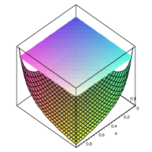
Figure 7: $r_{0}^{6}/b^{6}$ is plotted along height of above cube against $a$ and $c$. The flat surface is where $r_{0}=b$. Here , we take $\frac{L^{4}e^{\Phi}}{36}=1$.

The case $b^{6}/r_{0}^{6}<1$ seems to be interesting. It hints that D7 probe brane can rest at a non-trivial value of $r_{0}>b$, ahead of the problematic point of $r_{0}=b$. Since the probe brane do not venture through the strongly coupled region, predictions based on supergravity calculations should be reliable. For the configurations with these particular flux values, the open strings emanating from N D3 branes do have a place to end in the bulk.

References

-
[1]
J. M. Maldacena,
“The large N limit of superconformal field theories and supergravity,”
Adv. Theor. Math. Phys. 2 (1998) 231
[Int. J. Theor. Phys. 38 (1999) 1113]
[arXiv:hep-th/9711200].
O. Aharony, S. S. Gubser, J. M. Maldacena, H. Ooguri and Y. Oz, “Large N field theories, string theory and gravity,” Phys. Rept. 323 (2000) 183 [arXiv:hep-th/9905111]. -
[2]
E. Witten,
“Anti-de Sitter space and holography,”
Adv. Theor. Math. Phys. 2 (1998) 253
[arXiv:hep-th/9802150].
S. S. Gubser, I. R. Klebanov and A. M. Polyakov, “Gauge theory correlators from non-critical string theory,” Phys. Lett. B 428 (1998) 105 [arXiv:hep-th/9802109]. - [3] I. R. Klebanov and E. Witten, “Superconformal field theory on threebranes at a Calabi-Yau singularity,” Nucl. Phys. B 536 (1998) 199 [arXiv:hep-th/9807080].
-
[4]
J. P. Gauntlett, D. Martelli, J. Sparks and D. Waldram,
“Supersymmetric solutions of M-theory,”
Class. Quant. Grav. 21 (2004) 4335
[arXiv:hep-th/0402153].
J. P. Gauntlett, D. Martelli, J. Sparks and D. Waldram, “Sasaki-Einstein metrics on ,” Adv. Theor. Math. Phys. 8 (2004) 711 [arXiv:hep-th/0403002]. - [5] S. Benvenuti, S. Franco, A. Hanany, D. Martelli and J. Sparks, “An infinite family of superconformal quiver gauge theories with Sasaki-Einstein duals,” JHEP 0506, 064 (2005) [arXiv:hep-th/0411264].
- [6] M. Cvetič, H. Lu, D. N. Page and C. N. Pope, “New Einstein-Sasaki spaces in five and higher dimensions,” Phys. Rev. Lett. 95 (2005) 071101 [arXiv:hep-th/0504225].
- [7] D. Martelli and J. Sparks, “Toric Sasaki-Einstein metrics on ,” Phys. Lett. B 621 (2005) 208 [arXiv:hep-th/0505027].
- [8] S. Benvenuti and M. Kruczenski, “From Sasaki-Einstein spaces to quivers via BPS geodesics: ,” arXiv:hep-th/0505206.
- [9] S. Franco, A. Hanany, D. Martelli, J. Sparks, D. Vegh and B. Wecht, “Gauge theories from toric geometry and brane tilings,” arXiv:hep-th/0505211.
- [10] A. Butti, D. Forcella and A. Zaffaroni, “The dual superconformal theory for manifolds,” JHEP 0509, 018 (2005) [arXiv:hep-th/0505220].
- [11] I. R. Klebanov and E. Witten, “AdS/CFT correspondence and symmetry breaking,” Nucl. Phys. B 556 (1999) 89 [arXiv:hep-th/9905104].
- [12] E. Calabi, “Métriques Kaehlériennes et fibrés holomorphes,” Ann. Scient. Ec. Norm. Sup., 12 (1979), 269-294.
- [13] D. N. Page and C. N. Pope, “Inhomogeneous Einstein Metrics On Complex Line Bundles,” Class. Quant. Grav. 4 (1987) 213.
- [14] L. A. Pando Zayas and A. A. Tseytlin, “3-branes on spaces with topology,” Phys. Rev. D 63 (2001) 086006 [arXiv:hep-th/0101043].
- [15] S. S. Pal, “A new Ricci flat geometry,” Phys. Lett. B 614 (2005) 201 [arXiv:hep-th/0501012].
- [16] K. Sfetsos and D. Zoakos, “Supersymmetric solutions based on and ,” Phys. Lett. B 625 (2005) 135 [arXiv:hep-th/0507169].
- [17] O. Aharony, A. Hanany and B. Kol, “Webs of 5-branes, five dimensional field theories and grid diagrams,” JHEP 9801, 002 (1998) [arXiv:hep-th/9710116].
- [18] N. C. Leung and C. Vafa, “Branes and toric geometry,” Adv. Theor. Math. Phys. 2, 91 (1998) [arXiv:hep-th/9711013].
- [19] D. Martelli and J. Sparks, “Toric geometry, Sasaki-Einstein manifolds and a new infinite class of AdS/CFT duals,” arXiv:hep-th/0411238.
- [20] I. R. Klebanov and N. A. Nekrasov, “Gravity duals of fractional branes and logarithmic RG flow,” Nucl. Phys. B 574 (2000) 263 [arXiv:hep-th/9911096].
- [21] I. R. Klebanov and M. J. Strassler, “Supergravity and a confining gauge theory: Duality cascades and chiSB-resolution of naked singularities,” JHEP 0008 (2000) 052 [arXiv:hep-th/0007191].
- [22] C. P. Herzog, Q. J. Ejaz and I. R. Klebanov, “Cascading RG flows from new Sasaki-Einstein manifolds,” JHEP 0502 (2005) 009 [arXiv:hep-th/0412193].
- [23] B. A. Burrington, J. T. Liu, M. Mahato and L. A. Pando Zayas, “Towards supergravity duals of chiral symmetry breaking in Sasaki-Einstein cascading quiver theories,” JHEP 0507 (2005) 019 [arXiv:hep-th/0504155].
- [24] D. Gepner and S. S. Pal, “Branes in ,” Phys. Lett. B 622 (2005) 136 [arXiv:hep-th/0505039].
- [25] I. R. Klebanov and A. A. Tseytlin, “Gravity duals of supersymmetric gauge theories,” Nucl. Phys. B 578 (2000) 123 [arXiv:hep-th/0002159].
- [26] A. Dymarsky, I. R. Klebanov and N. Seiberg, arXiv:hep-th/0511254.
- [27] S. S. Gubser, C. P. Herzog and I. R. Klebanov, JHEP 0409, 036 (2004) [arXiv:hep-th/0405282].
- [28] G. Papadopoulos and A. A. Tseytlin, “Complex geometry of conifolds and 5-brane wrapped on 2-sphere,” Class. Quant. Grav. 18 (2001) 1333 [arXiv:hep-th/0012034].
- [29] A. Butti, M. Graña, R. Minasian, M. Petrini and A. Zaffaroni, “The baryonic branch of Klebanov-Strassler solution: A supersymmetric family of structure backgrounds,” JHEP 0503 (2005) 069 [arXiv:hep-th/0412187].
- [30] S. S. Gubser, “Einstein manifolds and conformal field theories,” Phys. Rev. D 59 (1999) 025006 [arXiv:hep-th/9807164].
- [31] A. Ceresole, G. Dall’Agata, R. D’Auria and S. Ferrara, “Spectrum of type IIB supergravity on : Predictions on SCFT’s,” Phys. Rev. D 61 (2000) 066001 [arXiv:hep-th/9905226].
- [32] L. A. Pando Zayas and A. A. Tseytlin, “3-branes on resolved conifold,” JHEP 0011 (2000) 028 [arXiv:hep-th/0010088].
- [33] S. Benvenuti and A. Hanany, “Conformal manifolds for the conifold and other toric field theories,” JHEP 0508, 024 (2005) [arXiv:hep-th/0502043].
- [34] D. Arean, D. E. Crooks and A. V. Ramallo, “Supersymmetric probes on the conifold,” JHEP 0411 (2004) 035 [arXiv:hep-th/0408210].
- [35] W. Fulton, “Introduction to Toric Varieties,” Princeton University Press, 1993.
- [36] N. R. Constable and R. C. Myers, “Exotic scalar states in the AdS/CFT correspondence,” JHEP 9911 (1999) 020 [arXiv:hep-th/9905081].
-
[37]
J. Babington, J. Erdmenger, N. J. Evans, Z. Guralnik and I. Kirsch,
“Chiral symmetry breaking and pions in non-supersymmetric gauge / gravity
duals,”
Phys. Rev. D 69 (2004) 066007
[arXiv:hep-th/0306018].
N. J. Evans and J. P. Shock, “Chiral dynamics from AdS space,” Phys. Rev. D 70 (2004) 046002 [arXiv:hep-th/0403279].
N. Evans, J. Shock and T. Waterson, “D7 brane embeddings and chiral symmetry breaking,” JHEP 0503 (2005) 005 [arXiv:hep-th/0502091].