Influence on electron coherence from quantum electromagnetic fields in the presence of conducting plates

Abstract

The influence of electromagnetic vacuum fluctuations in the presence of the perfectly conducting plate on electrons is studied with an interference experiment. The evolution of the reduced density matrix of the electron is derived by the method of influence functional. We find that the plate boundary anisotropically modifies vacuum fluctuations that in turn affect the electron coherence. The path plane of the interference is chosen either parallel or normal to the plate. In the vicinity of the plate, we show that the coherence between electrons due to the boundary is enhanced in the parallel configuration, but reduced in the normal case. The presence of the second parallel plate is found to boost these effects. The potential relation between the amplitude change and phase shift of interference fringes is pointed out. The finite conductivity effect on electron coherence is discussed.

I Introduction

Quantum coherence entails the existence of the interference effects amongst alternative histories of the quantum states. These effects are nevertheless not seen at the classical level. The suppression of quantum coherence can be viewed as the result of the unavoidable coupling to the environment, and thus leads to the emergence of the classical behavior in terms of incoherent mixtures. This environment-induced decoherence has been studied with the idea of quantum open systems by coarse-graining the environment where certain statistical measures are introduced ZU ; HA ; CAL1 ; CAL2 ; CAD . Thereby, this averaged effect appears as decoherence of the system of interest.

In modern cosmology, many efforts have been devoted to studying how primordial perturbations, created quantum-mechanically during inflation in the early universe, undergo the processes of decoherence when their low momentum modes cross out the horizon CAL2 ; ST ; RE . They then reenter the horizon during the radiation- or matter-dominated stage and thus act as the seeds of temperature inhomogeneities in the cosmic microwave background as well as the matter density inhomogeneities that lead to the large-scale structure formation. In addition, special attention has been paid to the possible observation of decoherence effects in mesoscopic physics such as the phenomena of quantum tunneling, which are affected by the coupling with a heat bath CAD . Recent revival of interest in the decoherence phenomenon is motivated by the study of the experimental realization of quantum computers in which the central obstacle has proven to preventing the degradation of the quantum coherence from the coupling of the computer to the environment NI . Understanding of the aforementioned problems relies on the deeper exploration of the decoherence dynamics driven by the environment.

The quantum decoherence due to the interaction with the environment has been discussed by considering the interference of the electron states coupled to quantum electromagnetic fields in vacuum FO ; MA . It has been shown that the electron interference pattern may be altered by particle creation and vacuum fluctuations of electromagnetic fields, and the change might be observed through the phase shift and the contrast change. However, imposition of the boundary conditions on quantum fields may result in the modification of vacuum fluctuations. The best-known example is the attractive Casimir force between two parallel conducting plates CA . This Casimir effect remains one of the least intuitive consequences of quantum field theory BA1 ; BA2 ; RO . Therefore, we expect that the presence of the boundary may further influence the electron interference and gives rise to observable effects. This type of the interference experiment can serve as a probe to understanding the nature of quantum fluctuations FO ; MA .

Here we study the decoherence dynamics of the electron coupled to quantum electromagnetic fields in the presence of the perfectly conducting plate. We employ the closed-time-path formalism to explore the evolution of the density matrix of the electron and fields SC . In recent years, this nonequilibrium formalism has been applied in particle physics and cosmology by one of us LEE . The reduced density matrix of the electron can then be derived with the method of influence functional, which takes account of backreaction. We assume that the electron is initially in a coherent superposition of two quantum states with their mean trajectory along the distinct paths. Then the interference fringes can be observed when these states are recombined. The phase shift and amplitude reduction of the electron interference influenced by quantum fields are obtained from the influence functional. The leading effect of the decoherence functional comes from the contribution evaluated along the prescribed electron’s classical trajectory defined by an applied potential. The validity of the approximation will be discussed FO ; BR . Note that this coherence reduction is given by the double surface integrals of the field strength correlation function defined in Minkowski spacetime as we will see later. In this sense, it shares similar features with the known Aharonov-Bohm effect where the phase shift of the electron interference in the presence of the classical static magnetic field depends on the magnetic flux in the region from which the electron is absent. Here we instead consider the effects on the interference from non-stationary quantum electromagnetic fields HS .

Our presentation is organized as follows. In Sec. II, we introduce the closed-time-path formalism for describing the evolution of the density matrix of a nonrelativistic electron interacting with quantum electromagnetic fields. We then employ the method of influence functional by tracing out the fields in the Coulomb gauge in which we find the evolution of the reduced density matrix for the electron with self-consistent backreaction. The effect of decoherence can be realized by constructing the decoherence functional from the influence functional under the classical approximation in Sec. III. In Sec. IV, we evaluate this decoherence functional for quantum electromagnetic fields in the presence of the perfectly conducting plate and study how coherence reduction of the electrons is affected by the modified vacuum fluctuations due to the boundary. The finite conductivity effect on electron coherence is discussed in Sec. V. The results are summarized in Sec. VI. In addition, in App. A, the nature of the gauge invariance in the decoherence functional is considered by explicitly computing it with an alternative gauge fixing. In App. B, we outline the method to convert a summation, which turns out to be slowly convergent, into a rapidly convergent form.

The Lorentz-Heaviside units with $\hbar=c=1$ will be adopted unless otherwise noted. The metric is $\eta^{\mu\nu}=\text{diag}(1,-1,-1,-1)$.

II influence functional approach

We consider the dynamics of a nonrelativistic electron interacting with quantum electromagnetic fields in the presence of the conducting plate. In the Coulomb gauge, the electric and magnetic fields can be expressed in terms of the vector potentials as:

$$\mathbf{E}=-\nabla A_{0}-\dot{\mathbf{A}}_{\mathrm{T}}\,,\qquad\mathbf{B}=\nabla\times\mathbf{A}_{\mathrm{T}}\,,$$ (1)

where $\mathbf{A}_{\mathrm{T}}$ is the transverse component of the potential satisfying the gauge condition, $\nabla\cdot\mathbf{A}_{\mathrm{T}}=0$. The time-component of the potential $A_{0}$ is not a dynamical field, but can be determined by the Gauss law with the instantaneous Coulomb Green’s function, which can be defined by $\nabla^{2}G(\mathbf{x},\mathbf{y})=-\,\delta^{3}(\mathbf{x}-\mathbf{y})$ subject to the boundary conditions. The charge and current densities for a nonrelativistic electron may take the form

$$\varrho(x;\mathbf{q}(t))=e\;\delta^{3}(\mathbf{x}-\mathbf{q}(t))\,,\qquad\mathbf{j}_{\mathrm{T}}(x;\mathbf{q}(t))=e\;\dot{\mathbf{q}}(t)\,\delta^{3}(\mathbf{x}-\mathbf{q}(t))\,,$$ (2)

with a coupling constant $e$. The current $\mathbf{j}_{\mathrm{T}}$ satisfies the transverse condition $\nabla\cdot\mathbf{j}_{\mathrm{T}}=0$. The Lagrangian of the electron-field system is then given by the transverse components of the vector potential as well as the coordinates $\mathbf{q}$ of the non-relativistic electron,

$$L[\mathbf{q},\mathbf{A}_{\mathrm{T}}]=\frac{1}{2}m\dot{\mathbf{q}}^{2}-V(\mathbf{q})-\frac{1}{2}\int\!d^{3}\mathbf{x}\,d^{3}\mathbf{y}\;\varrho(x;\mathbf{q})G(\mathbf{x},\mathbf{y})\varrho(y;\mathbf{q})+\int\!d^{3}\mathbf{x}\;\left[\frac{1}{2}(\partial_{\mu}\mathbf{A}_{\mathrm{T}})^{2}+\mathbf{j}_{\mathrm{T}}\cdot\mathbf{A}_{\mathrm{T}}\right]\,,$$ (3)

where an external potential $V$ is introduced so as to constrain the motion of the electron to the prescribed path, and the Coulomb electrostatic energy term is defined in the presence of the boundary BA2 .

The effect of electromagnetic fields on the electron interference can be realized by the diagonal elements of the reduced density matrix $\rho_{r}$, which is obtained by tracing out electromagnetic fields in the density matrix of the electron and fields. Let us consider that the initial density matrix at time $t_{i}$ can be factorized as

$$\rho(t_{i})=\rho_{e}(t_{i})\otimes\rho_{\mathbf{A}_{\mathrm{T}}}(t_{i})\,,$$ (4)

and that initially the fields are assumed in thermal equilibrium at temperature, $\beta^{-1}$ with the density matrix $\rho_{\mathbf{A}_{\mathrm{T}}}(t_{i})$ given by

$$\rho_{\mathbf{A}_{\mathrm{T}}}(t_{i})=e^{-\beta H_{\mathbf{A}_{\mathrm{T}}}}\,,$$ (5)

where $H_{\mathbf{A}_{\mathrm{T}}}$ is the Hamiltonian for the free electromagnetic fields, constructed from Eq. (3). Then the zero-temperature limit corresponding to the initial vacuum state of the fields can be reached by taking $\beta\rightarrow\infty$ limit. The electron-field system evolves unitarily according to

$$\rho(t_{f})=U(t_{f},t_{i})\,\rho(t_{i})\,U^{-1}(t_{f},t_{i})$$ (6)

with $U(t_{f},t_{i})$ the time evolution operator. Thereafter, the final state of the electron-field system in general becomes entangled due to the interaction between them. The interaction between the electron and fields will be assumed to be adiabatically switched on in the remote past with $t_{i}\to-\infty$, and then switched off in the remote future with $t_{f}\to\infty$. We then employ the closed-time-path formalism to describe the evolution of the density matrix of the electron-field. The reduced density matrix of the electron, by tracing out the fields, becomes

$$\rho_{r}(\mathbf{q}_{f},\tilde{\mathbf{q}}_{f},t_{f}) = \int\!d\mathbf{A}_{\mathrm{T}}\;\bigl{<}\mathbf{q}_{f},\mathbf{A}_{\mathrm{T}}\big{|}\rho(t_{f})\big{|}\tilde{\mathbf{q}}_{f},\mathbf{A}_{\mathrm{T}}\bigr{>}$$ (7)

$$= \int\!d\mathbf{A}_{\mathrm{T}}\int\!d\mathbf{q}_{1}\,d\mathbf{A}_{1\mathrm{T}}\int\!d\mathbf{q}_{2}\,d\mathbf{A}_{2\mathrm{T}}\;\bigl{<}\mathbf{q},\mathbf{A}_{\mathrm{T}}\big{|}U(t_{f},t_{i})\big{|}\mathbf{q}_{1},\mathbf{A}_{1\mathrm{T}}\bigr{>}$$

$$\qquad\qquad\times\bigl{<}\mathbf{q}_{1},\mathbf{A}_{1\mathrm{T}}\big{|}\rho(t_{i})\big{|}\mathbf{q}_{2},\mathbf{A}_{2,\mathrm{T}}\bigr{>}\bigl{<}\mathbf{q}_{2},\mathbf{A}_{2\mathrm{T}}\big{|}U^{-1}(t_{f},t_{i})\big{|}\tilde{\mathbf{q}},\mathbf{A}_{\mathrm{T}}\bigr{>}$$

$$= \int\!d\mathbf{q}_{1}\,d\mathbf{q}_{2}\int\!d\mathbf{A}_{\mathrm{T}}\,d\mathbf{A}_{1\mathrm{T}}\,d\mathbf{A}_{2\mathrm{T}}\int^{{\mathbf{q}}_{f}}_{\mathbf{q}_{1}}\!\mathcal{D}\mathbf{q}^{+}\int^{\tilde{\mathbf{q}}_{f}}_{\mathbf{q}_{2}}\!{\cal D}\mathbf{q}^{-}\int^{\mathbf{A}_{\mathrm{T}}}_{\mathbf{A}_{1\mathrm{T}}}\!\mathcal{D}\mathbf{A}_{\mathrm{T}}^{+}\int^{\mathbf{A}_{\mathrm{T}}}_{\mathbf{A}_{2\mathrm{T}}}\!\mathcal{D}\mathbf{A}_{\mathrm{T}}^{-}$$

$$\qquad\qquad\times\int^{\mathbf{A}_{1\mathrm{T}}}_{\mathbf{A}_{2\mathrm{T}}}\!\mathcal{D}\mathbf{A}_{\mathrm{T}}^{\beta}\;\exp\biggl{[}i\int_{t_{i}}^{t_{f}}dt\;L[\mathbf{q}^{+},\mathbf{A}_{\mathrm{T}}^{+}]-L[\mathbf{q}^{-},\mathbf{A}_{\mathrm{T}}^{-}]\biggr{]}$$

$$\qquad\qquad\qquad\qquad\qquad\times\exp\biggl{[}i\int_{t_{i}}^{t_{i}-i\beta}dt\;L_{0}[\mathbf{A}_{\mathrm{T}}^{\beta}]\biggr{]}\;\rho_{e}(\mathbf{q}_{1},\mathbf{q}_{2},t_{i})\,.$$

Here we have introduced an identity in terms of a complete set of eigenstates, $\big{|}\mathbf{q},\mathbf{A}_{\mathrm{T}}\bigr{>}$,

$$\int\!d^{3}\mathbf{q}\,d\mathbf{A}_{\mathrm{T}}\;\big{|}\mathbf{q},\mathbf{A}_{\mathrm{T}}\bigr{>}\bigl{<}\mathbf{q},\mathbf{A}_{\mathrm{T}}\big{|}=1\,,$$ (8)

with $\big{|}\mathbf{q},\mathbf{A}_{\mathrm{T}}\bigr{>}$ given by the direct product of the states of the electron and those of electromagnetic fields, namely, $\big{|}\mathbf{q},\mathbf{A}_{\mathrm{T}}\bigr{>}=\big{|}\mathbf{q}\bigr{>}\otimes\big{|}\mathbf{A}_{\mathrm{T}}\bigr{>}$. This identity has been inserted into the integrand so that the matrix element of the time evolution operator can be expressed by the path integral along either the forward or backward time evolution, represented by $\mathbf{q}^{+}$, $\mathbf{A}_{\mathrm{T}}^{+}$, and $\mathbf{q}^{-}$, $\mathbf{A}_{\mathrm{T}}^{-}$, respectively. The density matrix for the thermal state of fields corresponds to the evolution operator of the fields $\mathbf{A}_{\mathrm{T}}^{\beta}$ along a path parallel to the imaginary axis of complex time, and the time arguments of the field operators are limited to the range between the complex time $t_{i}$ and $t_{i}-i\beta$. Thus, the Green’s functions of the vector potentials possess the periodicity as the result of the cyclic property of the trace as well as the bosonic nature of the field operators.

Since the electron interacts with fields via a linear coupling, the fields can be traced out exactly. Thus, we obtain the influence functional for the electron by taking full account of the backreaction. The physics becomes more transparent when we write the evolution of the reduced density matrix in the following form

$$\rho_{r}(\mathbf{q}_{f},\tilde{\mathbf{q}}_{f},t_{f})=\int\!d^{3}\mathbf{q}_{1}\,d^{3}\mathbf{q}_{2}\;\mathcal{J}(\mathbf{q}_{f},\tilde{\mathbf{q}}_{f},t_{f};\mathbf{q}_{1},\mathbf{q}_{2},t_{i})\,\rho_{e}(\mathbf{q}_{1},\mathbf{q}_{2},t_{i})\,,$$ (9)

where the propagating function $\mathcal{J}(\mathbf{q}_{f},\tilde{\mathbf{q}}_{f},t_{f};\mathbf{q}_{1},\mathbf{q}_{2},t_{i})$ is

$$\mathcal{J}(\mathbf{q}_{f},\tilde{\mathbf{q}}_{f},t_{f};\mathbf{q}_{1},\mathbf{q}_{2},t_{i})=\int^{\mathbf{q}_{f}}_{\mathbf{q}_{1}}\!\!\mathcal{D}\mathbf{q}^{+}\!\!\int^{\tilde{\mathbf{q}}_{f}}_{\mathbf{q}_{2}}\!\!\mathcal{D}\mathbf{q}^{-}\;\exp\left[i\int_{t_{i}}^{t_{f}}dt\left(L_{e}[\mathbf{q}^{+}]-L_{e}[\mathbf{q}^{-}]\right)\right]\mathcal{F}[\mathbf{j}^{+}_{\mathrm{T}},\mathbf{j}^{-}_{\mathrm{T}}]\,,$$ (10)

and the electron Lagrangian $L_{e}[\mathbf{q}]$ is given by BA2

$$L_{e}\bigl{[}\mathbf{q}\bigr{]}=\frac{1}{2}m\dot{\mathbf{q}}^{2}-V(\mathbf{q})-\frac{1}{2}\int\!d^{3}\mathbf{x}\,d^{3}\mathbf{y}\;\varrho(x;\mathbf{q})\,G(\mathbf{x},\mathbf{y})\,\varrho(y;\mathbf{q})\,.$$ (11)

Here we introduce the influence functional $\mathcal{F}[\mathbf{j}^{+}_{\mathrm{T}},\mathbf{j}^{-}_{\mathrm{T}}]$,

$$\mathcal{F}[\mathbf{j}^{+}_{\mathrm{T}},\mathbf{j}^{-}_{\mathrm{T}}]=\exp\biggl{\{}-\frac{1}{2}\,e^{2}\int d^{4}x\!\!\! \int\!d^{4}x^{\prime}\Bigl{[}\;{\mathbf{j}^{+}_{\mathrm{T}}}_{i}(x;\mathbf{q}^{+}(t))\,\bigl{<}{\mathbf{A}^{+}_{\mathrm{T}}}^{i}(x){\mathbf{A}^{+}_{\mathrm{T}}}^{j}(x^{\prime})\bigr{>}\,{\mathbf{j}^{+}_{\mathrm{T}}}_{j}(x^{\prime};\mathbf{q}^{-}(t^{\prime}))\Bigr{.}\biggr{.}$$ (12)

$$-{\mathbf{j}^{+}_{\mathrm{T}}}_{i}(x;\mathbf{q}^{+}(t))\,\bigl{<}{\mathbf{A}^{+}_{\mathrm{T}}}^{i}(x){\mathbf{A}^{-}_{\mathrm{T}}}^{j}(x^{\prime})\bigr{>}\,{\mathbf{j}^{-}_{\mathrm{T}}}_{j}(x^{\prime};\mathbf{q}^{-}(t^{\prime}))$$

$$-{\mathbf{j}^{-}_{\mathrm{T}}}_{i}(x;\mathbf{q}^{-}(t))\,\bigl{<}{\mathbf{A}^{-}_{\mathrm{T}}}^{i}(x){\mathbf{A}^{+}_{\mathrm{T}}}^{j}(x^{\prime})\bigr{>}\,{\mathbf{j}^{+}_{\mathrm{T}}}_{j}(x^{\prime};\mathbf{q}^{+}(t^{\prime}))$$

$$\biggl{.}\Bigl{.}+\,{{\bf j}^{-}_{{\rm T}}}_{i}(x;{\bf q}^{-}(t))\,\bigl{<}{\mathbf{A}^{-}_{\mathrm{T}}}^{i}(x){\mathbf{A}^{-}_{\mathrm{T}}}^{j}(x^{\prime})\bigr{>}\,{\mathbf{j}^{-}_{\mathrm{T}}}_{j}(x^{\prime};\mathbf{q}^{-}(t^{\prime}))\Bigr{]}\biggr{\}}\,,$$

which contains full information about the influence of quantum electromagnetic fields on the electron, and is a highly nonlocal object. The Green’s functions of the vector potential are defined by

$$\bigl{<}{\mathbf{A}^{+}_{\mathrm{T}}}^{i}(x){\mathbf{A}^{+}_{\mathrm{T}}}^{j}(x^{\prime})\bigr{>} = \bigl{<}{\mathbf{A}_{\mathrm{T}}}^{i}(x){\mathbf{A}_{\mathrm{T}}}^{j}(x^{\prime})\bigr{>}\,\theta(t-t^{\prime})+\bigl{<}{\mathbf{A}_{\mathrm{T}}}^{j}(x^{\prime}){\mathbf{A}_{\mathrm{T}}}^{i}(x)\bigr{>}\,\theta(t^{\prime}-t)\,,$$

$$\bigl{<}{\mathbf{A}^{-}_{\mathrm{T}}}^{i}(x){\mathbf{A}^{-}_{\mathrm{T}}}^{j}(x^{\prime})\bigr{>} = \bigl{<}{\mathbf{A}_{\mathrm{T}}}^{j}(x^{\prime}){\mathbf{A}_{\mathrm{T}}}^{i}(x)\bigr{>}\,\theta(t-t^{\prime})+\bigl{<}{\mathbf{A}_{\mathrm{T}}}^{i}(x){\mathbf{A}_{\mathrm{T}}}^{j}(x^{\prime})\bigr{>}\,\theta(t^{\prime}-t)\,,$$

$$\bigl{<}{\mathbf{A}^{+}_{\mathrm{T}}}^{i}(x){\mathbf{A}^{-}_{\mathrm{T}}}^{j}(x^{\prime})\bigr{>} = \bigl{<}{\mathbf{A}_{\mathrm{T}}}^{j}(x^{\prime}){\mathbf{A}_{\mathrm{T}}}^{i}(x)\bigr{>}\equiv\mathrm{Tr}\left\{\rho_{\mathbf{A}_{\mathrm{T}}}\,{\mathbf{A}_{\mathrm{T}}}^{j}(x^{\prime}){\mathbf{A}_{\mathrm{T}}}^{i}(x)\right\}\,,$$

$$\bigl{<}{\mathbf{A}^{-}_{\mathrm{T}}}^{i}(x){\mathbf{A}^{+}_{\mathrm{T}}}^{j}(x^{\prime})\bigr{>} = \bigr{<}{\mathbf{A}_{\mathrm{T}}}^{i}(x){\mathbf{A}_{\mathrm{T}}}^{j}(x^{\prime})\bigr{>}\equiv\mathrm{Tr}\left\{\rho_{\mathbf{A}_{\mathrm{T}}}\,{\mathbf{A}_{\mathrm{T}}}^{i}(x){\mathbf{A}_{\mathrm{T}}}^{j}(x^{\prime})\right\}\,,$$ (13)

and can be explicitly constructed as long as electromagnetic fields are quantized subject to the boundary conditions. The retarded Green’s function and Hadamard function of vector potentials are defined respectively by

$$G_{R}^{ij}(x-x^{\prime}) = i\,\theta(t-t^{\prime})\,\bigl{<}\left[{\mathbf{A}_{\mathrm{T}}}^{i}(x),{\mathbf{A}_{\mathrm{T}}}^{j}(x^{\prime})\right]\bigr{>}\,,$$ (14)

$$G_{H}^{ij}(x-x^{\prime}) = \frac{1}{2}\,\bigl{<}\left\{{\mathbf{A}_{\mathrm{T}}}^{i}(x),{\mathbf{A}_{\mathrm{T}}}^{j}(x^{\prime})\right\}\big{>}\,.$$ (15)

Here the influence functional can be expressed in a more compact form in terms of its phase and modulus by:

$$\mathcal{F}[\,\mathbf{j}^{+}_{\mathrm{T}},\mathbf{j}^{-}_{\mathrm{T}}]=\exp\Big{\{}\mathcal{W}[\,\mathbf{j}^{+}_{\mathrm{T}},\mathbf{j}^{-}_{\mathrm{T}}]+i\,\Phi[\,\mathbf{j}^{+}_{\mathrm{T}},\mathbf{j}^{-}_{\mathrm{T}}]\Bigr{\}}\,,$$ (16)

where

$$\Phi[\,\mathbf{j}^{+}_{\mathrm{T}},\mathbf{j}^{-}_{\mathrm{T}}] =\frac{1}{2}\,e^{2}\!\!\int\!d^{4}x\!\!\int\!d^{4}x^{\prime}\Bigl{[}\,{\mathbf{j}^{+}_{\mathrm{T}}}_{i}(x;\mathbf{q}^{+})-{\mathbf{j}^{-}_{\mathrm{T}}}_{i}(x;\mathbf{q}^{-})\Bigr{]}G_{R}^{ij}(x-x^{\prime})\Bigl{[}\,{\mathbf{j}^{+}_{\mathrm{T}}}_{j}(x^{\prime};\mathbf{q}^{+})+{\mathbf{j}^{-}_{\mathrm{T}}}_{j}(x^{\prime};\mathbf{q}^{-})\Bigr{]}\,,$$

$$\mathcal{W}[\,\mathbf{j}^{+}_{\mathrm{T}},\mathbf{j}^{-}_{\mathrm{T}}] =-\frac{1}{2}\,e^{2}\!\!\int\!d^{4}x\!\!\int\!d^{4}x^{\prime}\Bigl{[}\,{\mathbf{j}^{+}_{\mathrm{T}}}_{i}(x;\mathbf{q}^{+})-{\mathbf{j}^{-}_{\mathrm{T}}}_{i}(x;\mathbf{q}^{-})\Bigr{]}G_{H}^{ij}(x-x^{\prime})\Bigl{[}\,{\mathbf{j}^{+}_{\mathrm{T}}}_{j}(x^{\prime};\mathbf{q}^{+})-{\mathbf{j}^{-}_{\mathrm{T}}}_{j}(x^{\prime};\mathbf{q}^{-})\Bigr{]}\,.$$ (17)

For a given initial state for the electron, the reduced density matrix for the electron at time $t_{f}$ can be obtained from Eq. (9) when the path integration over $\mathbf{q}^{\pm}$ in Eq. (10) is carried out. Explicitly written out, the reduced density operator now becomes

$$\rho_{r}(\mathbf{q}_{f},\tilde{\mathbf{q}}_{f},t_{f}) = \int\!d^{3}\mathbf{q}_{1}\,d^{3}\mathbf{q}_{2}\left[\int^{\mathbf{q}_{f}}_{\mathbf{q}_{1}}\!\!\mathcal{D}\mathbf{q}^{+}\!\!\int^{\tilde{\mathbf{q}}_{f}}_{\mathbf{q}_{2}}\!\!\mathcal{D}\mathbf{q}^{-}\;\exp\biggl{\{}i\int_{t_{i}}^{t_{f}}dt\left(L_{e}[\mathbf{q}^{+}]-L_{e}[\mathbf{q}^{-}]\right)\biggr{\}}\right.$$ (18)

$$\qquad\qquad\left.\,\times\,\exp\biggl{\{}\mathcal{W}[\mathbf{q}^{+},\mathbf{q}^{-}]\biggr{\}}\exp\biggl{\{}i\,\Phi[\mathbf{q}^{+},\mathbf{q}^{-}]\biggr{\}}\right]\rho_{e}(\mathbf{q}_{1},\mathbf{q}_{2},t_{i})\,.$$

Let us now consider the initial electron state vector $\bigl{|}\Psi(t_{i})\bigr{>}$ to be a coherent superposition of two localized states along worldlines $\mathcal{C}_{1}$ and $\mathcal{C}_{2}$, respectively, after they leave the beam splitter at the moment $t_{i}$,

$$\bigl{|}\Psi(t_{i})\bigr{>}=\bigl{|}\psi_{1}(t_{i})\bigr{>}+\bigl{|}\psi_{2}(t_{i})\bigr{>}\,.$$ (19)

The density matrix of the electron state is then given by

$$\rho_{e}(t_{i}) = \bigl{|}\Psi(t_{i})\bigr{>}\bigl{<}\Psi(t_{i})\bigr{|}$$ (20)

$$= \rho_{11}(t_{i})+\rho_{22}(t_{i})+\rho_{21}(t_{i})+\rho_{12}(t_{i})\,,$$ (21)

where $\rho_{mn}(t_{i})=\bigl{|}\psi_{m}(t_{i})\bigr{>}\bigl{<}\psi_{n}(t_{i})\bigr{|}$. The terms $\rho_{21}+\rho_{12}$ account for quantum interference, because when the density matrix is realized in the coordinate basis, we have

$$\bigl{<}\mathbf{q}_{i}\big{|}\rho_{e}(t_{i})\big{|}\mathbf{q}_{i}\bigr{>}=\left|\psi_{1}(\mathbf{q}_{i},t_{i})\right|^{2}+\left|\psi_{2}(\mathbf{q}_{i},t_{i})\right|^{2}+2\,\mathfrak{Re}\left\{\psi_{2}^{*}(\mathbf{q}_{i},t_{i})\psi_{1}^{\vphantom{*}}(\mathbf{q}_{i},t_{i})\right\}\,,$$ (22)

which expresses the probability of finding an electron at $(t_{i},\mathbf{q}_{i})$ in the superposed state. Therefore, at time $t_{f}$, when the electron states are recombined at the location $\mathbf{q}_{f}$, the electron interference pattern can be described by the diagonal elements of the reduced density matrix $\bigl{<}\mathbf{q}_{f}\big{|}\rho_{r}(t_{f})\big{|}\mathbf{q}_{f}\bigr{>}=\rho_{r}(\mathbf{q}_{f},\mathbf{q}_{f},t_{f})$ .

III decoherence functional in the classical approximation

The expression (18) of the reduced density matrix at time $t_{f}$ accounts for the full quantum effects of the electron, but the corresponding path integral can not be carried out without invoking further approximation FO . In general, the interaction with quantum electromagnetic fields is expected to perturb the electron’s trajectory in a stochastic way about its mean value, and to cause the electron wavefunction to spread YU . It also fluctuates the phase of the wavefunction such that the phase coherence between electrons is lost.

Now considering the electron as a well-defined wave packet, its mean trajectory follows the classical path constrained by an appropriate external potential $V(\mathbf{q})$. The effect of the Coulomb electrostatic attraction due to presence of the boundary is usually small in the typical experiment configuration FO , and then its influence on the trajectory can be ignored. In addition, the backreaction from quantum field fluctuations, which is of the order of the weak coupling $e^{2}/4\pi$ in the influence functional also has the ignorable correction to the classical paths as expected. Furthermore, the finite spread of the wave packet of the electron state, due to uncertainties on both position and momentum, can be legitimately neglected as long as the electron’s de Broglie wavelength, $\lambda_{\mathrm{dB}}$ is much shorter than the characteristic length scale associated with the accuracy of the measurement $l$. Thus, as long as $l\gg\lambda_{\mathrm{dB}}$, the wave packet can be viewed as it is sharply peaked in the electron’s position and momentum, and thus its quantum effects can be ignored FO . As such, the leading effect of the decoherence can be obtained by evaluating the propagating function (10) along a prescribed classical path of the electrons. Thereby, the diagonal components of the reduced density matrix $\rho_{r}(\mathbf{q}_{f},\mathbf{q}_{f},t_{f})$ now becomes

$$\rho_{r}(\mathbf{q}_{f},\mathbf{q}_{f},t_{f})=\bigl{|}\psi_{1}(\mathbf{q}_{f},t_{f})\bigr{|}^{2}+\bigl{|}\psi_{2}(\mathbf{q}_{f},t_{f})\bigr{|}^{2}+2\,e^{\mathcal{W}[\,\bar{\mathbf{j}}^{1}_{\mathrm{T}},\bar{\mathbf{j}}^{2}_{\mathrm{T}}]}\;\mathfrak{Re}\left\{e^{i\,\Phi[\,\bar{\mathbf{j}}^{1}_{\mathrm{T}},\bar{\mathbf{j}}^{2}_{\mathrm{T}}]}\psi_{1}^{\vphantom{*}}(\mathbf{q}_{f},t_{f})\,\psi_{2}^{*}(\mathbf{q}_{f},t_{f})\right\}\,,$$ (23)

where the $\mathcal{W}$ and $\Phi$ functionals are evaluated along the classical trajectories, $\mathcal{C}_{1}$ and $\mathcal{C}_{2}$. $\bar{\mathbf{j}}^{1,2}_{\mathrm{T}}$ is the classical current along the respective paths. The evolution of the electron states $\psi_{1,2}(\mathbf{q}_{f},t_{f})$ is governed by the Lagrangian $L_{e}$ in Eq. (11) due to the ignorable backreaction effects.

The exponent of the modulus of the influence functional $\mathcal{W}$, determined by the Hadamard function of vector potentials, reveals decoherence between coherent electrons, while its phase functional $\Phi$, related to the retarded Green’s function, results in an overall phase shift for the electron interference pattern. Both effects arise from the interaction with quantum fields. The decoherence functional can be obtained from the expectation value of the anti-commutator of the vector potentials. However, in the semiclassical Langevin equation to describe the stochastic dynamics of the particle coupled to quantum fields, the Hadamard function also determines the noise correlation function from quantum field fluctuations which cause the stochastic behavior of the particle’s trajectory WU2 . Thus, we can conclude that coherence reduction of the electrons is driven by field fluctuations. On the other hand, the phase functional, which is related to the retarded Green’s function for the commutator of vector potentials, link to the backreaction dissipation in the Langevin equation on the dynamics of the particle WU2 . Thus, the phase shift may result from the backreaction dissipation from quantum fields through particle creation that influences the mean trajectory of the electrons. These two effects in the Langevin equation obey the underlying fluctuation-dissipation theorem. In this aspect, the effects of quantum decoherence and the phase shift are also likely related by the fluctuation-dissipation theorem. However, very little work has been done to establish this relation. It will be investigated in our future work. Here we only concentrate on the effect of quantum decoherence induced by vacuum fluctuations of electromagnetic fields.

In the classical approximation, with the help of Eqs. (2) and (17), the decoherence factor, the $\mathcal{W}$ functional, can be expressed as

$$\mathcal{W}=-\frac{e^{2}}{2}\,\oint_{C}dx_{j}\oint_{C}dx^{\prime}_{k}\,G_{H}^{jk}(x,x^{\prime})\,,$$ (24)

where $\mathbf{x},\mathbf{x}^{\prime}\in C=C_{1}-C_{2}$ and $j,k=1,2,3$. The curves $C_{1,2}$ are the projection of the worldlines $\mathcal{C}_{1,2}$ onto the hypersurface normal to the time axis in Minkowski spacetime. Then, it is a straightforward calculation to re-write the $\mathcal{W}$ functional in terms of the fields $\mathbf{E}$ and $\mathbf{B}$ in a manifestly gauge invariant way,

$$\mathcal{W}=-\frac{e^{2}}{8}\int_{\mathcal{C}}\!da_{\mu\nu}^{\vphantom{{}^{\prime}}}\int_{\mathcal{C}}\!da^{\prime}_{\rho\sigma}\;\bigl{<}\left\{F^{\mu\nu}(x),F^{\rho\sigma}(x^{\prime})\right\}\bigr{>}\,.$$ (25)

Apparently, the decoherence factor involves double surface integrals of the expectation value of the anticommutator between the field strength $F^{\mu\nu}$ as the area element $d\sigma^{\mu\nu}$ of the integral is bounded by a closed worldline of the electron $\mathcal{C}$ in Minkowski spacetime. The closed worldline $\mathcal{C}=\mathcal{C}_{1}-\mathcal{C}_{2}$ can be thought of as moving electron along its path $C_{1}$ in the forward time direction and then along the path $C_{2}$ in the backward time direction. By means of the 4-dimensional Stokes’ theorem, we can write the $\mathcal{W}$ functional (25) as

$$\mathcal{W}=-\frac{e^{2}}{2}\oint_{\mathcal{C}}\!dx^{\vphantom{{}^{\prime}}}_{\mu}\,\oint_{\mathcal{C}}\!dx^{\prime}_{\nu}\;G_{H}^{\mu\nu}(x,x^{\prime})\,,$$ (26)

which involves the Hadamard function of the covariant vector potentials. It is consistent with the result in Ref. FO .

Note that although the expectation value of the vector potential $\langle A^{\mu}(x)\rangle$ in the electromagnetic vacuum state vanishes even in the presence of the boundary, the fluctuations of fields are non-zero in general. The decoherence effect in Eq. (25) emerges as the result of the double surface integrals of the non-vanishing field correlations in Minkowski spacetime. Thus the decoherence is found sensitive to the field strength in the region where the electron is excluded. In this aspect, it may be regarded as the generalization to the Aharonov-Bohm effect with time-independent classical electromagnetic fields. In contrast, in our case, the decoherence effect is essentially driven by the non-static features of quantum fields.

IV Evaluation of the $\mathcal{W}$ functional

IV.1 unbounded space

As for illustration, let us start by considering the $\mathcal{W}_{0}$ functional for the unbounded space where electromagnetic fields are initially in the vacuum state MA . The trajectory of the electrons can be dictated by an external potential along the prescribed paths. The velocity of the electron in the $x$ direction $v_{x}$ is assumed to be constant, while the motion in the $z$ direction varies with time. Thus, the respective worldlines of electrons are given by $\mathcal{C}_{1,2}=(t,v_{x}t,0,\pm\zeta(t))$. The path function $\zeta(t)$ is required to be sufficiently smooth to avoid enormous photon production from the kinked corners and it may take the form,

$$\zeta(t)=R\,e^{-\frac{t^{2}}{T^{2}}}\,,$$ (27)

where $2R$ is the effective path separation and $2T$ is the effective flight time. The vector potential can be expressed by the creation and annihilation operators as:

$$\mathbf{A}_{\mathrm{T}}(x)=\int\!\frac{d^{3}\mathbf{k}}{(2\pi)^{\frac{3}{2}}}\,\frac{1}{\sqrt{2\omega}}\sum_{\lambda=1,2}\hat{\boldsymbol{\epsilon}}_{\lambda}(\mathbf{k})a_{\lambda}(\mathbf{k})\,e^{i\mathbf{k}\cdot\mathbf{x}-i\omega t}+\text{H.C.}\,$$ (28)

with $\omega=\left|\mathbf{k}\right|$. The polarization unit vectors $\hat{\boldsymbol{\epsilon}}_{\lambda}$ obey the transversality condition given by,

$$\sum_{\lambda=1,2}\hat{\boldsymbol{\epsilon}}^{i}_{\lambda}(\mathbf{k})\,\hat{\boldsymbol{\epsilon}}^{j}_{\lambda}(\mathbf{k})=\delta^{ij}-\frac{k^{i}k^{j}}{\left|\mathbf{k}\right|^{2}}\,.$$ (29)

Since the $\mathcal{W}$ functional in Eq. (26) reveals manifest Lorentz invariance, it proves more convenient to boost to a frame $\mathfrak{S}$ moving with the velocity $u=(1,v_{x},0,0)$ at $y=z=0$, in which the electrons are seen to have transverse motion in the $z$ direction only. Then, the $\mathcal{W}_{0}$ functional (24) can be obtained by a straightforward calculation of the $z$–$z$ component of the vector potential Hadamard function with the help of the mode expansion (28), and reduces to

$$\mathcal{W}_{0}=-2e^{2}\int\!\!\frac{d^{3}\mathbf{k}}{(2\pi)^{3}}\frac{1}{2\omega}\left[1-\frac{k_{z}^{2}}{\omega^{2}}\right]\left|\int\!\!dt\,\dot{\zeta}\cos\left(k_{z}\zeta\right)e^{i\omega t}\right|^{2}\,,$$ (30)

where $\dot{\zeta}=d\zeta/dt$. We further simplify the calculation by applying the dipole approximation, $\cos\left(k_{z}\zeta\right)\simeq 1$, consistent with the non-relativistic limit. By using the path function (27), the decoherence functional $\mathcal{W}_{0}$ ends up with

$$\mathcal{W}_{0} \simeq -2e^{2}\int\!\!\frac{d^{3}\mathbf{k}}{(2\pi)^{3}}\frac{1}{2\omega}\left[1-\frac{k_{z}^{2}}{\omega^{2}}\right]\left|\int\!dt\;\dot{\zeta}\;e^{i\omega t}\right|^{2}$$ (31)

$$= -\frac{e^{2}}{4\pi}R^{2}T^{2}\int_{-\infty}^{\infty}dk_{z}\int_{\left|k_{z}\right|}^{\infty}d\omega\left(\omega^{2}-k_{z}^{2}\right)e^{-\frac{1}{2}\omega^{2}T^{2}}$$

$$= -\frac{2e^{2}}{3\pi}\frac{R^{2}}{T^{2}}\left(\frac{1}{c^{2}}\right)\,,$$

which is finite without the ultraviolet divergence. The absence of the potential ultraviolet divergence can be seen from the corresponding Fourier transform of the path function (27) where the contribution from the high frequency modes with $\omega\gtrsim\mathcal{O}(1/T)$ is exponentially suppressed. The result free of ultraviolet divergence is quite general for the smooth path function with the finite flight time.

In the nonrelativistic limit, since the transverse component of the electron velocity $v_{z}$ is about $10^{-2}c$ in a typical interference experiment, the decoherence factor $\mathcal{W}_{0}$, proportional to $v^{2}_{z}$, will be of the order of $10^{-5}$ to $10^{-6}$. Therefore, it is hardly to detect the loss of the interference contrast due to vacuum fluctuations of quantum fields in this unbounded case.

IV.2 presence of the single plate

Now we consider the decoherence effect between the coherent electrons under the influence of quantum electromagnetic fields in the bounded region. In the presence of the perfectly conducting plate, the tangential component of the electric field $\mathbf{E}$ as well as the normal component of the magnetic field $\mathbf{B}$ on the plate surface vanish. When the plate is placed at the $z=0$ plane, the boundary conditions of the fields $\mathbf{E}$ and $\mathbf{B}$ on the plate give rise to

$$A_{0}=0\,,\qquad\text{and}\qquad A_{x}=A_{y}=0\,,$$ (32)

which lead to

$$\frac{\partial{A}_{z}}{\partial z}=0$$ (33)

as the result of the Coulomb gauge. The transverse vector potential $\mathbf{A}_{\mathrm{T}}$ in the $z>0$ region is given by BA2 ,

$$\mathbf{A}_{\mathrm{T}}(x) = \int\!\frac{d^{2}\mathbf{k}_{\parallel}}{2\pi}\!\int_{0}^{\infty}\!\frac{dk_{z}}{(2\pi)^{1/2}}\;\frac{2}{\sqrt{2\omega}}\biggl{\{}a_{1}(\mathbf{k})\,\hat{\mathbf{k}}_{\parallel}\times\hat{\mathbf{z}}\,\sin k_{z}z\biggr{.}$$ (34)

$$\quad\quad\quad\biggl{.}+\;a_{2}(\mathbf{k})\left[i\,\hat{\mathbf{k}}_{\parallel}\left(\frac{k_{z}}{\omega}\right)\sin k_{z}z-\hat{\mathbf{z}}\left(\frac{k_{\parallel}}{\omega}\right)\cos k_{z}z\right]\biggr{\}}\;e^{i\mathbf{k}_{\parallel}\cdot\mathbf{x}_{\parallel}-i\omega t}+\text{H.C.}\,,$$

where the circumflex identifies unit vectors. The position vector $\mathbf{x}$ is denoted by $\mathbf{x}=(\mathbf{x}_{\parallel},z)$ where $\mathbf{x}_{\parallel}$ is the components parallel to the plate. Similarly, the wave vector is expressed by $\mathbf{k}=(\mathbf{k}_{\parallel},k_{z})$ with $\omega^{2}=k_{\parallel}^{2}+k_{z}^{2}$. The creation and annihilation operators obey the commutation relations

$$[a_{{\lambda}^{\vphantom{l}}}^{\vphantom{\dagger}}(\mathbf{k}),a_{\lambda^{\prime}}^{\dagger}(\mathbf{k}^{\prime})]=\delta_{{\lambda}{\lambda}^{\prime}}\,\delta(\mathbf{k}_{\parallel}^{\vphantom{{}^{\prime}}}-\mathbf{k}^{\prime}_{\parallel})\,\delta(k_{z}^{\vphantom{{}^{\prime}}}-k^{\prime}_{z})\,,$$ (35)

and otherwise are zero.

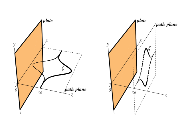
Figure 1: Two different orientations of the electron path plane relative to the conducting plate.

The path plane on which the electrons travel can be either parallel or perpendicular to the plate. When the path plane is normal to the conducting plate as shown in Fig. 1, the electron worldlines are given by $\mathcal{C}_{1,2}=(t,v_{x}t,0,z_{0}\pm\zeta(t))$. We will choose a frame $\mathfrak{S}$ which moves along the worldline $(t,v_{x}t,0,z_{0})$ and has the same orientation as the laboratory frame. In this frame, the electrons are seen to have sideways motion in the $z$ direction only. Then the $\mathcal{W}_{\perp}$ functional depends on the $z$–$z$ component of the vector potential Hadamard function, which is given by

$$G_{H}^{zz}(x,x^{\prime})=\frac{1}{2}\int\frac{d^{3}\bf{k}}{(2\pi)^{3}}\frac{1}{2\omega}\left(\frac{k_{\parallel}}{\omega}\right)^{2}\cos k_{z}z\,\cos k_{z}z^{\prime}\;e^{i\mathbf{k}_{\parallel}^{\vphantom{{}^{\prime}}}\cdot(\mathbf{x}_{\parallel}^{\vphantom{{}^{\prime}}}-\mathbf{x}^{\prime}_{\parallel})-i\omega(t-t^{\prime})}+\text{C.C.}\,.$$ (36)

Thus, the decoherence functional $\mathcal{W}_{\perp}$ can be obtained as:

$$\mathcal{W}_{\perp} = -\frac{e^{2}}{2}\left(\int_{C_{1}}dz\int_{C_{1}}dz^{\prime}+\int_{C_{2}}dz\int_{C_{2}}dz^{\prime}-\int_{C_{1}}dz\int_{C_{2}}dz^{\prime}-\int_{C_{2}}dz\int_{C_{1}}dz^{\prime}\right)G_{H}^{zz}(x,x^{\prime})$$ (37)

$$= -\frac{e^{2}}{4}\int\!dt\,\dot{\zeta}\;dt^{\prime}\,\dot{\zeta}^{\prime}\!\int\frac{d^{3}\bf{k}}{(2\pi)^{3}}\;\frac{1}{2\omega}\left(\frac{k_{\parallel}}{\omega}\right)^{2}\biggl{\{}\cos k_{z}(z_{0}+\zeta)\cos k_{z}(z_{0}+\zeta^{\prime})\biggr{.}$$

$$\qquad\qquad\qquad\qquad+\cos k_{z}(z_{0}-\zeta)\cos k_{z}(z_{0}-\zeta^{\prime})+\cos k_{z}(z_{0}-\zeta)\cos k_{z}(z_{0}+\zeta^{\prime})$$

$$\biggl{.}\qquad\qquad\qquad\qquad+\cos k_{z}(z_{0}+\zeta)\cos k_{z}(z_{0}-\zeta^{\prime})\biggr{\}}e^{-i\omega(t-t^{\prime})}+\text{C.C.}$$

$$= -2e^{2}\int\!\frac{d^{3}\bf{k}}{(2\pi)^{3}}\;\frac{1}{2\omega}\left[1-\frac{k_{z}^{2}}{\omega^{2}}\right]\biggl{[}1+e^{i2k_{z}z_{0}}\biggr{]}\left|\int\!dt\;\dot{\zeta}\cos k_{z}\zeta\;e^{-i\omega t}\right|^{2}\,.$$

Then, under the dipole approximation, we arrive at:

$$\mathcal{W}_{\perp}=\mathcal{W}_{0}\left\{1+\frac{3}{32\xi^{3}}\left[-4\xi+\sqrt{2\pi}\left(1+4\xi^{2}\right)e^{-2\xi^{2}}\operatorname{Erfi}(\sqrt{2}\xi)\right]\right\}$$ (38)

with the path function given by Eq. (27). Here the corrections to the decoherence functional due to the presence of the conducting plate is expressed in terms of the ratio of the effective distance of the electrons to the plate over the parameter $T$, i.e., $\xi=z_{0}/T$. The imaginary error function $\operatorname{Erfi}(z)$ is defined by

$$\operatorname{Erfi}(z)\equiv-i\operatorname{Erf}(i\,z)=\frac{2}{\sqrt{\pi}}\int^{z}_{0}\!ds\,e^{s^{2}}\,.$$ (39)

Asymptotically, the ratio $\mathcal{W}_{\perp}/\left|\mathcal{W}_{0}\right|$ is given by

$$\frac{\mathcal{W}_{\perp}}{\left|\mathcal{W}_{0}\right|}=\begin{cases}-2+\displaystyle\frac{8}{5}\xi^{2}+\mathcal{O}(\xi^{4})\,,&\xi\to 0\,;\\ &\\ -1-\displaystyle\frac{3}{16}\frac{1}{\xi^{4}}+\mathcal{O}(\frac{1}{\xi^{6}})\,,&\xi\to\infty\,.\end{cases}$$ (40)

As shown in Fig. 2, the effects of coherence reduction by vacuum fluctuations in the presence of the boundary are strikingly deviated from that without the boundary. It can be understood by the fact that the presence of the perfectly conducting plate modifies zero-point fluctuations of the fields which manifest themselves so as to influence the dynamics of decoherence in the electron interference.

In particular, when the path plane lies normal to the plate, we find that the modified vacuum fluctuations due to the boundary further reduce the electron coherence, then in turn suppress the contrast of the interference fringes for all values of $\xi$. It is found that for small $\xi$, $\mathcal{W}_{\perp}\approx 2\mathcal{W}_{0}$ MA . To understand this, here we provide an explanation in contrast to the fictitious dipole interpretation suggested by Ref. MA . Let us note that, in the reference frame $\mathfrak{S}$, the relevant component of the electromagnetic fields in this case is the $\mathbf{E}_{z}$ field, which is perpendicular to the conducting plate. The effect of the neutral conducting plate can be achieved by placing an image charge at the location symmetrical to the original charge with respect to the plate. The image charge shall carry the opposite sign to the real one as required by the boundary conditions. As such, the $\mathbf{E}_{z}$ field produced by the image charge is almost the same as that by the original one so as to make the total $\mathbf{E}_{z}$ field near the surface twice that in the unbounded case. Thus, the decoherence effect is doubled MA . However, when the ratio $\xi$ increases, the suppression of electron coherence is alleviated as expected and finally reduces to the result without the boundary in the limit $\xi\rightarrow\infty$. Also note that the ratio $\xi$ can not infinitesimally go to zero because $z_{0}$ has to be larger than $R$ to constrain the electrons on one side of the plate.

Figure 2: The decoherence functional $\mathcal{W}$ for the single-plate boundary as a function of the ratio $\xi=z_{0}/T$.

On the other hand, when the path plane lies parallel to the conducting plate, here the electron worldlines are given by $\mathcal{C}_{1,2}=(t,v_{x}t,\pm\zeta(t),z_{0})$. The same reference frame $\mathfrak{S}$ is chosen so that the electrons are seen to move in the $y$ direction. Then, the $y$–$y$ component of the vector potential Hadamard function becomes relevant to the $\mathcal{W}_{\parallel}$ and it is given by,

$$G_{H}^{yy}(x,x^{\prime})=\frac{1}{2}\int\frac{d^{3}\mathbf{k}}{(2\pi)^{3}}\frac{1}{2\omega}\left\{\sin^{2}\chi+\frac{k_{z}^{2}}{\omega^{2}}\cos^{2}\chi\right\}\sin k_{z}z\,\sin k_{z}z^{\prime}\;e^{i\mathbf{k}_{\parallel}^{\vphantom{{}^{\prime}}}\cdot(\mathbf{x}_{\parallel}^{\vphantom{{}^{\prime}}}-\mathbf{x}^{\prime}_{\parallel})-i\omega(t-t^{\prime})}+\text{C.C.}\,,$$ (41)

where $\chi$ is the angle between $\hat{\mathbf{y}}$ and $\hat{\mathbf{k}}_{\parallel}$. We then obtain the decoherence functional $\mathcal{W}_{\parallel}$,

$$\mathcal{W}_{\parallel} = -e^{2}\left(\int_{C_{1}}dy\int_{C_{1}}dy^{\prime}-\int_{C_{1}}dy\int_{C_{2}}dy^{\prime}\right)G_{H}^{yy}(x,x^{\prime})$$ (42)

$$= -2e^{2}\int\!\frac{d^{3}\mathbf{k}}{(2\pi)^{3}}\;\frac{1}{2\omega}\left[1-\frac{k_{y}^{2}}{\omega^{2}}\right]\biggl{[}1-e^{i2k_{z}z_{0}}\biggr{]}\left|\int\!dt\;\dot{\zeta}\cos k_{z}\zeta\;e^{-i\omega t}\right|^{2}\,.$$

Following the same approximation to obtain Eq. (38), the $\mathcal{W}_{\parallel}$ now is given by

$$\mathcal{W}_{\parallel}=\mathcal{W}_{0}\left\{1-\frac{3}{64\xi^{3}}\left[4\xi\left(1+4\xi^{2}\right)-\sqrt{2\pi}\left(1+16\xi^{4}\right)e^{-2\xi^{2}}\operatorname{Erfi}(\sqrt{2}\xi)\right]\right\}\,,$$ (43)

and asymptotically $\mathcal{W}_{\parallel}/\left|\mathcal{W}_{0}\right|$ is obtained as

$$\frac{\mathcal{W}_{\parallel}}{\left|\mathcal{W}_{0}\right|}=\begin{cases}-\displaystyle\frac{16}{5}\xi^{2}+\frac{144}{35}\xi^{4}+\mathcal{O}(\xi^{6})\,,&\xi\to 0\,;\\ &\\ -1-\displaystyle\frac{3}{16}\frac{1}{\xi^{4}}+\mathcal{O}(\frac{1}{\xi^{6}})\,,&\xi\to\infty\,.\end{cases}$$ (44)

In contrast to the perpendicular case, near the plate surface where $\xi\ll 1$, the electron coherence is enhanced. The loss of coherence originally due to vacuum fluctuations in the unbounded space is almost completely compensated by the induced fluctuations due to the boundary, especially in the limit of $\xi\to 0$. For small $\xi$, we find that $\mathcal{W}_{\parallel}\approx 0$. Apparently, in the reference frame $\mathfrak{S}$, the $\mathbf{E}_{y}$ component, which is parallel to the plate, is crucial. As required by the boundary conditions, the presence of the image charge renders the $\mathbf{E}_{y}$ field almost zero near the plate surface, leading to the vanishing field fluctuations. Thus, it is not so surprising that the electron coherence is restored near the plate surface. However, when the ratio $\xi$ is much greater than unity, we expect that the orientation of the path plane becomes irrelevant. The influence of the boundary on electron coherence is negligible. The decoherence effect reduces to the result in the perpendicular configuration, and then to that in the unbounded case in the limit $\xi\rightarrow\infty$. We can see from Fig. 2 that the presence of the boundary makes the electrons more coherent for small $\xi$, but less coherent for large $\xi$ in the parallel configuration.

The presence of the conducting plate anisotropically modifies the electromagnetic vacuum fluctuations that in turn influence the dynamics of the electrons coupled to the fields. In Ref. YU , the authors investigate the Brownian motion of the test particle coupled to quantized electromagnetic fields. An anisotropical modification in the mean squared fluctuations of the velocity near the conducting plate is found. Since the mean squared fluctuations of the velocity reflect vacuum fluctuations of fields, it is concluded that close to the plate, the electromagnetic vacuum fluctuations are suppressed in the direction transverse to the plate, compared to the unbounded case, while fluctuations are enhanced in the longitudinal direction. This is consistent with our results.

IV.3 presence of the double plates

In the presence of double plates, we place the second plate at $z=a$, in addition to the one at $z=0$. Thus, the transverse vector potential $\mathbf{A}_{\mathrm{T}}$ for the bounded region between the $z=0$ and $z=a$ planes can be expressed by BA1

$$\mathbf{A}_{\mathrm{T}}(x) =\sqrt{\frac{2}{a}}\;{\sum_{n=0}^{\infty}}^{\prime\prime}\!\int\!\frac{d^{2}\mathbf{k}_{\parallel}}{2\pi}\frac{1}{\sqrt{2\omega_{n}}}\biggl{\{}a_{1}(\mathbf{k}_{\parallel},n)\,\hat{\mathbf{k}}_{\parallel}\times\hat{\mathbf{z}}\,\sin\frac{n\pi}{a}z\biggr{.}$$

$$\qquad\biggl{.}+\;a_{2}(\mathbf{k}_{\parallel},n)\left[i\,\hat{\mathbf{k}}_{\parallel}\left(\frac{n\pi}{\omega_{n}a}\right)\sin\frac{n\pi}{a}z-\hat{\mathbf{z}}\left(\frac{k_{\parallel}}{\omega_{n}}\right)\cos\frac{n\pi}{a}z\right]\biggr{\}}e^{i\mathbf{k}_{\parallel}\cdot\mathbf{x}_{\parallel}-i\omega_{n}t}+\text{H.C.}\,.$$ (45)

The double prime on $\sum$ assigns an extra normalization factor $1/\sqrt{2}$ to the $n=0$ mode. The discrete frequencies $\omega_{n}$ of the allowed modes for the double-plate boundary are

$$\omega_{n}^{2}=k_{\parallel}^{2}+\left(\frac{n\pi}{a}\right)^{2}\,.$$ (46)

Moreover, the creation and annihilation operators obey the commutation relations

$$[a_{{\lambda}^{\vphantom{l}}}^{\vphantom{\dagger}}(\mathbf{k}_{\parallel}^{\vphantom{{}^{\prime}}},n),a_{{\lambda}^{\prime}}^{\dagger}(\mathbf{k}^{\prime}_{\parallel},n^{\prime})]=\delta_{{\lambda}{\lambda}^{\prime}}\,\delta_{nn^{\prime}}\,\delta(\mathbf{k}^{\vphantom{{}^{\prime}}}_{\parallel}-\mathbf{k}^{\prime}_{\parallel})\,,$$ (47)

and otherwise vanish.

As in the single plate case, we consider that the path plane lies either parallel or perpendicular to the plates. In the perpendicular case, we assume that the electrons move along their worldlines, described by $\mathcal{C}_{1,2}=(t,v_{x}t,0,\frac{a}{2}\pm\zeta(t))$, where the path function $\zeta$ is given by Eq. (27). As before, we choose the frame $\mathfrak{S}$ with $z_{0}=a/2$, in which the electrons are observed to move in the $z$ direction. Thereby, the relevant component of the vector potential Hadamard function is the $z$–$z$ component,

$$G_{H}^{zz}(x,x^{\prime})=\frac{1}{2a}\sum_{n=-\infty}^{\infty}\int\!\frac{d^{2}\mathbf{k}_{\parallel}}{(2\pi)^{2}}\frac{1}{2\omega_{n}}\left(\frac{k_{\parallel}}{\omega_{n}}\right)^{2}\!\!\cos\frac{n\pi}{a}z\,\cos\frac{n\pi}{a}z^{\prime}\;e^{i\mathbf{k}_{\parallel}^{\vphantom{{}^{\prime}}}\cdot(\mathbf{x}_{\parallel}^{\vphantom{{}^{\prime}}}-\mathbf{x}^{\prime}_{\parallel})-i\omega_{n}(t-t^{\prime})}+\text{C.C.}\,.$$ (48)

Thus, the decoherence functional $\mathcal{W}_{\perp}$ now becomes

$$\mathcal{W}_{\perp}=-\frac{2e^{2}}{a}\sum_{n=\text{even}}\!\int\!\frac{d^{2}\bf{k}_{\parallel}}{(2\pi)^{2}}\frac{1}{2\omega_{n}}\left[1-\frac{n^{2}\pi^{2}}{\omega_{n}^{2}a^{2}}\right]\left|\int\!dt\;\dot{\zeta}\cos\frac{n\pi}{a}\zeta\;e^{-i\omega_{n}t}\right|^{2}\,.$$ (49)

Then, by applying the dipole approximation, it reduces to

$$\mathcal{W}_{\perp} \simeq -\frac{e^{2}}{2}\,\frac{R^{2}}{T\,a}\sum_{n=-\infty}^{\infty}\left[\left|n\right|\varsigma\,e^{-\frac{1}{2}\,n^{2}\varsigma^{2}}+\sqrt{\frac{\pi}{2}}\left(1-n^{2}\varsigma^{2}\right)\operatorname{Erfc}(\frac{\left|n\right|\varsigma}{\sqrt{2}})\right]\,,$$ (50)

with $\varsigma=2\pi T/a$. The complementary error function, $\operatorname{Erfc}(z)$, is defined as

$$\operatorname{Erfc}(z)\equiv 1-\operatorname{Erf}(z)=\frac{2}{\sqrt{\pi}}\int^{\infty}_{z}\!ds\;e^{-s^{2}}\,.$$ (51)

Let us now consider the limit $\varsigma\gg 1$, that is, $a\ll T$, where the plate separation is much smaller than the flight time. In this limit, the decoherence functional (50) is dominated by the $n=0$ term with $\operatorname{Erfc}(0)=1$, while the $n\neq 0$ terms are exponentially suppressed due to large $\varsigma$. Hence, the $\mathcal{W}_{\perp}$ functional can be approximated by

$$\mathcal{W}_{\perp} \simeq -\frac{e^{2}}{2}\,\frac{R^{2}}{T\,a}\left\{\sqrt{\frac{\pi}{2}}+\frac{2}{\pi}\left(\frac{a}{T}\right)\,e^{-2\pi^{2}\frac{T^{2}}{a^{2}}}+\cdots\right\}\,.$$ (52)

It can be seen that the result is very small for $R<a\ll T$. However, compared with the unbounded case, the ratio $\mathcal{W}_{\perp}/\left|\mathcal{W}_{0}\right|$ is

$$\frac{\mathcal{W}_{\perp}}{\left|\mathcal{W}_{0}\right|}=-\frac{3\pi^{\frac{3}{2}}}{4\sqrt{2}}\,\frac{T}{a}\ll-1\,,$$ (53)

thus more significantly degrading electron coherence. Nonetheless, the ratio $a/T$ can not indefinitely go to zero, and is bounded by $2R/T$ from below since the plate separation can not be smaller than the path separation.

As the ratio $a/T$ becomes much greater than unity, the value of the decoherence functional reduces to the unbounded case. To see it, we convert Eq. (49) to a form suited for this limit with the method outlined in App. B. The $\mathcal{W}_{\perp}$ functional now takes the form

$$\mathcal{W}_{\perp} = -\frac{e^{2}}{2}\,\frac{R^{2}}{T\,a}\left\{\frac{8}{3\varsigma}+4\sum_{n=1}^{\infty}\left[-\frac{\varsigma}{2\pi^{2}}\frac{1}{n^{2}}+\frac{1}{(2\pi)^{\frac{1}{2}}}\frac{1}{n^{3}}\left(n^{2}+\frac{\varsigma^{2}}{4\pi^{2}}\right)e^{-2\left(\frac{n\pi}{\varsigma}\right)^{2}}\operatorname{Erfi}(\sqrt{2}\,\frac{n\pi}{\varsigma})\right]\right\}$$ (54)

$$\simeq -e^{2}\,\frac{R^{2}}{T\,a}\left\{\frac{4}{3\varsigma}+\frac{\varsigma^{3}}{2\pi^{4}}\sum_{n=1}^{\infty}\frac{1}{n^{4}}\,e^{-2\left(\frac{\pi}{\varsigma}\right)^{2}n^{2}}+\cdots\right\}\,,\qquad\text{for $\varsigma\ll 1$}\,.$$

Here the last line is obtained by Taylor-expanding the terms in the square bracket. Thus, we have, in the limit $a\gg T$,

$$\mathcal{W}_{\perp}\simeq\mathcal{W}_{0}\left\{1+6\,\frac{T^{4}}{a^{4}}\,e^{-\frac{a^{2}}{2T^{2}}}+\cdots\right\}\,.$$ (55)

The first term is the contribution to the decoherence effect from vacuum fluctuations without the boundary, while the second term, although exponentially small, is the correction due to the presence of the double plates.

In Fig. 3, the ratio of the $\mathcal{W}_{\perp}$ functional over the absolute value of $\mathcal{W}_{0}$ is plotted for a very wide range of $a/T$. It is shown that vacuum fluctuations arising from the presence of the plates always degrades electron coherence for the perpendicular case as expected from the single plate case. In addition, introducing the second plate seems to boost fluctuations so as to further reduce the electron coherence significantly in the limit of $a/T\ll 1$, where the effect of the boundary becomes important.

Figure 3: The decoherence functional $\mathcal{W}$ for the double-plate boundary as a function of the ratio $a/T$.

In the parallel case, the electron worldlines are given by $\mathcal{C}_{1,2}=(t,v_{x}t,\pm\zeta,\frac{a}{2})$, and the same reference frame $\mathfrak{S}$ is chosen. Then in this frame the electrons are observed to move in the $y$ direction only. The contributing component of the vector potential Hadamard function is the $y$–$y$ component, given by:

$$G_{H}^{yy}(x,x^{\prime}) = \frac{1}{2a}\sum_{n=-\infty}^{\infty}\int\!\frac{d^{2}\mathbf{k}_{\parallel}}{(2\pi)^{2}}\frac{1}{2\omega_{n}}\biggl{\{}\sin^{2}\chi\,\sin\frac{n\pi}{a}z\,\sin\frac{n\pi}{a}z^{\prime}\biggr{.}$$ (56)

$$\biggl{.}+\left(\frac{n\pi}{\omega_{n}a}\right)^{2}\cos^{2}\chi\,\sin\frac{n\pi}{a}z\,\sin\frac{n\pi}{a}z^{\prime}\biggr{\}}e^{i\mathbf{k}_{\parallel}^{\vphantom{{}^{\prime}}}\cdot(\mathbf{x}_{\parallel}^{\vphantom{{}^{\prime}}}-\mathbf{x}^{\prime}_{\parallel})-i\omega_{n}(t-t^{\prime})}+\text{C.C.}\,,$$

where $\chi$ is the angle between $\hat{\mathbf{y}}$ and $\hat{\mathbf{k}}_{\parallel}$. Then, the decoherence functional $\mathcal{W}_{\parallel}$ is

$$\mathcal{W}_{\parallel}=-\frac{2e^{2}}{a}\sum_{n=\text{odd}}\!\int\!\frac{d^{2}\mathbf{k}_{\parallel}}{(2\pi)^{2}}\frac{1}{2\omega_{n}}\left[1-\frac{k_{y}^{2}}{\omega_{n}^{2}}\right]\left|\int\!dt\;\dot{\zeta}\cos k_{y}\,\zeta\;e^{-i\omega_{n}t}\right|^{2}\,.$$ (57)

Therefore, we obtain

$$\mathcal{W}_{\parallel}\simeq-\frac{e^{2}}{2}\,\frac{R^{2}}{T\,a}\sum_{n=1}^{\infty}\left[q_{n}\,\varsigma\,e^{-\frac{1}{2}q_{n}^{2}\varsigma^{2}}+\sqrt{\frac{\pi}{2}}\left(1+q_{n}^{2}\varsigma^{2}\right)\operatorname{Erfc}(\frac{q_{n}\varsigma}{\sqrt{2}})\right]\,,$$ (58)

with $q_{n}=n-1/2$. The same approximation we invoked in the perpendicular case can be applied here. The result of Eq. (58) is shown in Fig. 3, which reveals the similar features as in the single-plate case.

In the limit $\varsigma\gg 1$ or $T\gg a$, the dominant contribution to Eq. (58) comes from the $n=1$ term, and the decoherence functional can be further approximated by

$$\mathcal{W}_{\parallel}\simeq-\pi\,e^{2}\,\frac{R^{2}}{a^{2}}\,e^{-\frac{\pi^{2}}{2}\frac{T^{2}}{a^{2}}}\,,$$ (59)

which is exponentially small as $a/T\rightarrow 0$. It can be interpreted as the fact that the presence of the double-plate boundary may further suppress vacuum fluctuations in the direction parallel to the conducting plates as compared with the single-plate case, and thus enhances the electron coherence. An interesting feature of the double-plate case can be seen from Fig. 3 that the plot has a rather wide plateau for the small $a/T$ up to the value $a/T\sim 1$ within which no appreciable loss of electron coherence could be observed. It can be understood by the fact that when both plates come close to one another, the dominant contribution to Eq. (57) comes from the $n=1$ modes. Since their frequencies, $\omega_{1}\geq\pi/a$ for all ${\bf k}_{\parallel}$ obtained from Eq. (46), have become sufficiently high due to small $a$, the contributions of those modes are exponentially suppressed as can be seen from the absolute value of the integral in Eq. (57). This is quite different from the single-plate case.

Next, in the other limit $\varsigma\ll 1$ or $T\ll a$, it is straightforward to show that the $\mathcal{W}_{\parallel}$ functional now is given by,

$$\mathcal{W}_{\parallel} = -\frac{e^{2}}{2}\frac{R^{2}}{T\,a}\left\{\frac{8}{3\varsigma}+\sum_{n=1}^{\infty}(-1)^{n}\left[\frac{\varsigma}{\pi^{2}}\frac{1}{n^{2}}+\frac{4}{\varsigma}-\sqrt{\frac{\pi}{2}}\frac{8\pi}{n^{3}\varsigma^{2}}\left(n^{4}+\frac{\varsigma^{4}}{16\pi^{4}}\right)e^{-\frac{1}{2}\left(\frac{n\pi}{\varsigma}\right)^{2}}\operatorname{Erfi}(\sqrt{2}\frac{n\pi}{\varsigma})\right]\right\}$$ (60)

$$\simeq -\frac{e^{2}}{2}\frac{R^{2}}{T\,a}\left\{\frac{8}{3\varsigma}-\frac{\varsigma^{3}}{\pi^{4}}\sum_{n=1}^{\infty}(-1)^{n}\frac{1}{n^{4}}+\cdots\right\}\,,\qquad\text{for $\varsigma\ll 1$}\,.$$

Then, as $a/T\gg 1$, we have

$$\mathcal{W}_{\parallel}\simeq\mathcal{W}_{0}\left\{1+\frac{7\pi^{4}}{120}\,\frac{T^{4}}{a^{4}}+\cdots\right\}\,.$$ (61)

The first term of the decoherence functional comes from the influence of vacuum fluctuations without the boundary, while the second term arises from the presence of the double-plate.

Some remarks are in place. In the perpendicular configuration, the correction of the decoherence effect in Eq. (55) takes the exponential form for the large $a/T$. This is due to the fact that the double plate geometry provides a length scale $2a$, the plate separation, in the $z$ direction, thus introducing this scale into the $z$–$z$ components of the correlation functions. However, in the parallel configuration, there is no such a length scale in this direction. Thus, it ends up with the correction of the form of the power of the ratio $a/T$ in the above expression. In addition, for the result of the $\mathcal{W}_{\parallel}$ in either the single-plate or the double-plate case, as shown in Figs. 2 and 3 respectively, we observe that $\mathcal{W}_{\parallel}\simeq 0$ for small $z_{0}/T$ or $a/T$, and then $\mathcal{W}_{\parallel}$ approaches the value of $\mathcal{W}_{0}$ from below in the region of large $z_{0}/T$ or $a/T$. Thus, $\mathcal{W}_{\parallel}$ must intersect with $\mathcal{W}_{0}$ at some value of the ratio, and exist a local minimum in these cases.

V Brief discussion on finite conductivity effect

The finite conductivity effect on electron coherence due to electromagnetic fields near conducting plates have been discussed AN . In the interference experiment, when the electron moves parallel to the surface of the conducting plate with velocity $\mathbf{v}$, the induced surface charge in the conductor is expected to move along with the electron with the same velocity. As a result, the electric field inside the conductor in the direction of motion of the electron arises, and is to be $\mathbf{E}\propto e\,\mathbf{v}$. The induced current then is given by the Ohmic law, $\mathbf{J}=\sigma\mathbf{E}$, where $\sigma$ is the conductivity of the conductor. The presence of the current inside the conductor leads to energy loss due to Joule heating at a rate $P_{\rm{Joule}}$, roughly given by $P_{\mathrm{Joule}}\propto\mathbf{E}\cdot\mathbf{J}\propto(e^{2}/\sigma)\,v^{2}$ with $v=\left|\mathbf{v}\right|$. We assume that the electron moves at a distance $d$ from the surface of the conducting plate. Then the $d$–dependence of the Joule energy loss rate $P_{\mathrm{Joule}}$ is given in Ref. BO in the context of classical electrodynamics,

$$P_{\mathrm{Joule}}=\frac{1}{16\pi}\biggl{(}\frac{e^{2}}{d}\biggr{)}\biggl{(}\frac{v^{2}}{\sigma d^{2}}\biggr{)}\,.$$ (62)

For a resistive plate boundary at room temperature, the effect of Joule heating is found to play a key role on electron coherence in the interference experiment AN . The observed contrast of electron interference fringes decreases due to large energy loss from Ohmic resistance as the electron moves close to the boundary. However, that is a different channel of decoherence from what we study. Here we consider electron decoherence due to vacuum fluctuations of electromagnetic fields with the perfectly conducting plate boundary. In contrast, when the electron travels parallel to the conducting plate, electron coherence is enhanced instead as it gets closer to the boundary since the electric field, responsible for decoherence, is vanishing along the plate surface. It is of interest to estimate the value of conductivity $\sigma$ at which the decoherence dynamics due to vacuum fluctuations is not masked by Ohmic dissipation. In the typical interference experiment, the electron moves with low velocities, and its velocity change is determined by the electric field with an overall factor $e/m$. The mean squared velocity dispersion owing to vacuum fluctuations of the fields along the surface of the conducting plate is given by YU ,

$$\langle\Delta v^{2}\rangle=\frac{1}{4\pi^{2}}\biggl{(}\frac{e^{2}}{d}\biggr{)}\biggl{(}\frac{1}{m\,d}\biggr{)}\biggl{(}\frac{1}{m}\biggr{)}\,,$$ (63)

where the parameter $d$ is the distance of the electron to the plate. As long as the Joule energy loss during the electron’s flight time $T$ is much smaller than average energy fluctuations obtained from the velocity fluctuations above, the effect from the finite conductivity of the boundary can be ignored for the large enough conductivity given by:

$$\sigma\approx\frac{\pi}{2}\frac{mvL}{d}\approx 10^{20}\biggl{(}\frac{v}{10^{-4}c}\biggr{)}\biggl{(}\frac{10\,\mu\mathrm{m}}{d}\biggr{)}\biggl{(}\frac{L}{10\,\mathrm{cm}}\biggr{)}\mathrm{s}^{-1}\,,$$ (64)

with the electron’s path length $L=v\,T$. This required high conductivity roughly about two orders of magnitude larger than that of Copper at room temperature can possibly be achieved for metallic material at low temperature.

VI Summary and Conclusion

In the present work, we investigate the influence of zero-point fluctuations of quantum electromagnetic fields in the presence of the perfectly conducting plates on electrons. The effects of modified vacuum fluctuations can be observed through the electron interference experiment, and are manifested in the form of the amplitude change and phase shift of the interference fringes. Here we first of all outline the closed-time-path formalism to describe the evolution of the density matrix of the electron and fields. Then, the method of influence functional is employed by tracing out the fields in the Coulomb gauge from which we find the evolution of the reduced density matrix of the electron with self-consistent backreaction.

Under the classical approximation with the prescribed electron’s trajectory dictated by an external potential, we find that the exponent of the modulus of the influence functional describes the extent of the amplitude change of the interference contrast, and its phase results in an overall shift for the interference pattern. In addition, it is known that the semiclassical Langevin equation for considering the stochastic behavior of the particle coupled to quantum fields, involves backreaction dissipation in terms of the retarded Green’s function of fields as well as the accompanying stochastic noise with the noise correlation function given by its Hadamard function. These two effects are in general linked by the fluctuation-dissipation theorem WU2 . Thus, we may conclude that reduction of coherence is driven by field fluctuations while the phase shift results from backreaction dissipation through particle creation that influences the mean trajectory of the electron.

We evaluate the decoherence functional of the electrons with the boundary on quantum electromagnetic fields. The boundary conditions can be imposed by the presence of either a single plate or double parallel plates. In each case, the path plane on which the electrons travel for the interference experiment can be parallel or perpendicular to the plate(s). It is found that the effects of coherence reduction of the electrons by zero-point fluctuations with the boundary are strikingly deviated from that without the boundary. Thus, the presence of the conducting plate anisotropically modifies electromagnetic vacuum fluctuations that in turn influence the decoherence dynamics of the electrons. In particular, as the electrons are close to the plate, electron coherence is enhanced in the case where the path plane of the electrons is parallel to the plate. It is resulted from the suppression of zero-point fluctuations due to the boundary in the direction transverse to the plate. On the other hand, the electron coherence is reduced in the perpendicular configuration where zero-point fluctuations are boosted instead along the direction longitudinal to the plate. In addition, in the presence of double parallel plates boundary, zero-point fluctuations seems to make the electrons more coherent in the parallel configuration, but less coherent in the perpendicular one, as compared with the single-plate boundary.

Thus, the loss of decoherence of the electrons can be understood from zero-point fluctuations of electromagnetic fields given by the Hadamard function of vector potentials. On the other hand, the backreaction dissipation through photon emission can influence the mean trajectory of the electron, and in turn leads to the phase shift on the electron inference pattern through the retarded Green’s function. We wish in our future work to address the issue of the relation between the amplitude change and phase shift of interference fringes via the fluctuation-dissipation theorem, which might be testable in the interference experiment.

Appendix A the decoherence functional in the Feynman gauge

The decoherence functional $\mathcal{W}$ obtained in the Coulomb gauge can be cast into the gauge invariant expression (25). Here, we illustrate the nature of the gauge invariance by explicitly computing the decoherence functional with an alternative gauge fixing. We choose the Feynman gauge as an example, and then the Green’s functions of the vector potentials in the presence of the conducting plates can be obtained by the method of the image charge BR .

In the following discussion, we assume that path function $\zeta(t)$ is required to be sufficiently smooth and an even function of time $t$. The range of time $t$ extends from $-\infty$ to $+\infty$ such that, for the motion of the electron to be physically meaningful, the first time derivative of the path function must vanish at endpoints, that is, $\dot{\zeta}(-\infty)=\dot{\zeta}(+\infty)=0$ in this case.

A.1 the single plate

Consider a conducting plate lying at the $z=0$ plane. The $\mathcal{W}$ functional, with the help of the image method, is given by

$$\mathcal{W} = -\frac{e^{2}}{2}\oint_{\mathcal{C}}dx_{\mu}\oint_{\mathcal{C}}dx^{\prime}_{\nu}\frac{1}{4\pi^{2}}\left[\frac{\eta^{\mu\nu}}{\triangle t^{2}-\triangle x_{\parallel}^{2}-(z-z^{\prime})^{2}}-\frac{\left(\eta^{\mu\nu}+2n^{\mu}n^{\nu}\right)}{\triangle t^{2}-\triangle x_{\parallel}^{2}-(z+z^{\prime})^{2}}\right]$$ (65)

$$= \mathcal{W}^{(0)}+\mathcal{W}^{(R)}\,,$$

where $n^{\mu}=(0,0,0,1)$ is a unit vector normal to the plate. $\triangle t$ and $\triangle x_{\parallel}$ denote $t-t^{\prime}$ and $x-x^{\prime}$, respectively. Apparently, the $\mathcal{W}$ functional can be written as the sum of $\mathcal{W}^{(0)}$ from the vacuum fluctuations in the unbounded space and $\mathcal{W}^{(R)}$ from the contribution of the image charge that accounts for the presence of the conducting plate. The $\mathcal{W}^{(0)}$ term is explicitly given by,

$$\mathcal{W}^{(0)} = -\frac{e^{2}}{8\pi^{2}}\,\oint_{\mathcal{C}}dx_{\mu}\oint_{\mathcal{C}}dx^{\prime}_{\nu}\;\frac{\eta^{\mu\nu}}{\triangle t^{2}-\triangle x_{\parallel}^{2}-(z-z^{\prime})^{2}}$$ (66)

$$= \frac{e^{2}}{4}\left[\int_{\mathcal{C}_{1}}\int_{\mathcal{C}_{1}}+\int_{\mathcal{C}_{2}}\int_{\mathcal{C}_{2}}-\int_{\mathcal{C}_{1}}\int_{\mathcal{C}_{2}}-\int_{\mathcal{C}_{2}}\int_{\mathcal{C}_{1}}\right]dt\,dt^{\prime}\;(1-\mathbf{v}\cdot\mathbf{v}^{\prime})$$

$$\qquad\qquad\times\int\!\frac{d^{3}\mathbf{k}}{(2\pi)^{3}}\;\frac{1}{2\omega}\Bigl{[}e^{i\mathbf{k}^{\vphantom{{}^{\prime}}}_{\parallel}\cdot(\mathbf{x}^{\vphantom{{}^{\prime}}}_{\parallel}-\mathbf{x}^{\prime}_{\parallel})+ik_{z}(z-z^{\prime})-i\omega(t-t^{\prime})}+\text{C.C.}\Bigr{]}\,,$$

where $\mathbf{v}=d\mathbf{x}/dt$ and $\mathcal{C}=\mathcal{C}_{1}-\mathcal{C}_{2}$. We only consider the case that the path plane is perpendicular to the plate and denote the decoherence functional as $\mathcal{W}_{\perp}$. The extension to the parallel case is straightforward.

The worldlines of the electrons are chosen to take the form, $\mathcal{C}_{1,2}=(t,v_{x}t,0,z_{0}\pm\zeta(t))$. The Lorentz invariance of the decoherence functional enables us to choose the frame $\mathfrak{S}$ moving along a straight line described by $(t,v_{x}t,0,z_{0})$ defined in Sec. V. Observed from this reference frame, the electrons are to move only transversally in the $z$ direction. Then, the $\mathcal{W}_{\perp}^{(0)}$ term reduces to

$$\mathcal{W}_{\perp}^{(0)} =e^{2}\left\{\int\!dt\,dt^{\prime}\;(1-\dot{\zeta}\dot{\zeta}^{\prime})\int\!\frac{d^{3}\mathbf{k}}{(2\pi)^{3}}\;\frac{1}{2\omega}\;e^{-ik_{z}(\zeta-\zeta^{\prime})+i\omega(t-t^{\prime})}\right.$$

$$\qquad\left.\qquad\qquad\qquad-\int\!dt\,dt^{\prime}\;(1+\dot{\zeta}\dot{\zeta}^{\prime})\int\!\frac{d^{3}\mathbf{k}}{(2\pi)^{3}}\;\frac{1}{2\omega}\;e^{-ik_{z}(\zeta+\zeta^{\prime})+i\omega(t-t^{\prime})}\right\}$$ (67)

$$=2e^{2}\left\{\int\!dt\,dt^{\prime}\int\!\frac{d^{3}\mathbf{k}}{(2\pi)^{3}}\;\frac{1}{2\omega}\,\sin k_{z}\zeta\,\sin k_{z}\zeta^{\prime}\,e^{i\omega(t-t^{\prime})}\right.$$

$$\qquad\qquad\qquad\qquad\left.-\int\!dt\,dt^{\prime}\;\dot{\zeta}\dot{\zeta}^{\prime}\int\!\!\frac{d^{3}\mathbf{k}}{(2\pi)^{3}}\;\frac{1}{2\omega}\,\cos k_{z}\zeta\,\cos k_{z}\zeta^{\prime}\,e^{i\omega(t-t^{\prime})}\right\}\,.$$ (68)

We then perform the integration by parts on the first term of Eq. (68) and obtain

$$\mathcal{W}_{\perp}^{(0)}=-2e^{2}\int\!\frac{d^{3}\mathbf{k}}{(2\pi)^{3}}\;\frac{1}{2\omega}\left[1-\frac{k_{z}^{2}}{\omega^{2}}\right]\left|\int\!dt\;\dot{\zeta}\cos k_{z}\zeta\,e^{i\omega t}\right|^{2}\,.$$ (69)

Following the similar procedures leads to the $\mathcal{W}_{\perp}^{(R)}$ functional given by,

$$\mathcal{W}_{\perp}^{(R)} =\frac{e^{2}}{8\pi^{2}}\oint_{\mathcal{C}}\!dx_{\mu}\oint_{\mathcal{C}}\!dx_{\nu}\sum_{n=-\infty}^{\infty}\frac{\eta^{\mu\nu}-n^{\mu}n^{\nu}}{\triangle t^{2}-\triangle x_{\parallel}^{2}-(z-z^{\prime}-2na)^{2}}$$

$$=-2e^{2}\int\!\frac{d^{3}\mathbf{k}}{(2\pi)^{3}}\;\frac{1}{2\omega}\,e^{-2ik_{z}z_{0}}\left[1-\frac{k_{z}^{2}}{\omega^{2}}\right]\left|\int\!dt\;\dot{\zeta}\cos k_{z}\zeta\,e^{i\omega t}\right|^{2}\,.$$ (70)

Then, putting Eqs. (69) and (70) together, the $\mathcal{W}_{\perp}$ functional becomes

$$\mathcal{W}_{\perp}=-2e^{2}\int\!\frac{d^{3}\mathbf{k}}{(2\pi)^{3}}\;\frac{1}{2\omega}\biggl{[}1+e^{-2ik_{z}z_{0}}\biggr{]}\biggl{[}1-\frac{k_{z}^{2}}{\omega^{2}}\biggr{]}\left|\int\!dt\;\dot{\zeta}\cos(k_{z}\,\zeta)e^{i\omega t}\right|^{2}\,,$$ (71)

which is of the same form as Eq. (37) derived in the Coulomb gauge.

A.2 the double-plate

We now turn to the case with two conducting plates at the $z=0$ and $z=a$ planes, respectively. The $\mathcal{W}$ functional is given by

$$\mathcal{W} = -\frac{e^{2}}{8\pi^{2}}\oint_{\mathcal{C}}dx_{\mu}\oint_{\mathcal{C}}dx^{\prime}_{\nu}\sum_{n=-\infty}^{\infty}\left[\frac{\eta^{\mu\nu}}{\triangle t^{2}-\triangle x_{\parallel}^{2}-(z-z^{\prime}-2na)^{2}}-\frac{\eta^{\mu\nu}+2n^{\mu}n^{\nu}}{\triangle t^{2}-\triangle x_{\parallel}^{2}-(z+z^{\prime}-2na)^{2}}\right]$$ (72)

$$= \mathcal{W}^{(I)}+\mathcal{W}^{(I\!I)}\,,$$

in terms of a sum of the contributions from the image charges. The $\mathcal{W}^{(I)}$ can be written explicitly as

$$\mathcal{W}^{(I)} =-\frac{e^{2}}{8\pi^{2}}\oint_{\mathcal{C}}\!dx_{\mu}\oint_{\mathcal{C}}\!dx_{\nu}\sum_{n=-\infty}^{\infty}\frac{\eta^{\mu\nu}}{\triangle t^{2}-\triangle x_{\parallel}^{2}-(z-z^{\prime}-2na)^{2}}$$

$$=\frac{e^{2}}{2}\left[\int_{\mathcal{C}_{1}}\int_{\mathcal{C}_{1}}+\int_{\mathcal{C}_{2}}\int_{\mathcal{C}_{2}}-\int_{\mathcal{C}_{1}}\int_{\mathcal{C}_{2}}-\int_{\mathcal{C}_{2}}\int_{\mathcal{C}_{1}}\right]dt\,dt^{\prime}\;(1-\mathbf{v}\cdot\mathbf{v}^{\prime})$$ (73)

$$\qquad\qquad\qquad\times\sum_{n=-\infty}^{\infty}\int\frac{d^{3}\mathbf{k}}{(2\pi)^{3}}\;\frac{1}{2\omega}\left[e^{i\mathbf{k}^{\vphantom{{}^{\prime}}}_{\parallel}\cdot(\mathbf{x}^{\vphantom{{}^{\prime}}}_{\parallel}-\mathbf{x}^{\prime}_{\parallel})+ik_{z}(z-z^{\prime}-2na)-i\omega(t-t^{\prime})}+\text{C.C.}\right]\,,$$

with the velocity $\mathbf{v}=d\mathbf{x}/dt$ and the closed path given by $\mathcal{C}=\mathcal{C}_{1}-\mathcal{C}_{2}$. The integration over $k_{z}$ can be carried out by the identity

$$\sum_{n=-\infty}^{\infty}e^{2ik_{z}na}=\frac{\pi}{a}\sum_{m=-\infty}^{\infty}\delta(k_{z}-\frac{m\pi}{a})\,.$$ (74)

We consider the case that the path plane of the electrons is perpendicular to the plates and the worldlines of electrons are described by $\mathcal{C}_{1,2}=(t,v_{x}t,0,\frac{a}{2}\pm\zeta(t))$. We evaluate the decoherence functional $\mathcal{W}_{\perp}$ in the frame $\mathfrak{S}$ with $z_{0}=a/2$. Therefore, the $\mathcal{W}_{\perp}$ function is simplified to

$$\mathcal{W}_{\perp}^{(I)} = \frac{e^{2}}{2a}\sum_{n=-\infty}^{\infty}\left\{\int\!dtdt^{\prime}\;(1-\dot{\zeta}\dot{\zeta}^{\prime})\int\!\frac{d^{2}\mathbf{k}_{\parallel}}{(2\pi)^{2}}\;\frac{1}{2\omega_{n}}\,e^{-i\frac{n\pi}{a}(\zeta-\zeta^{\prime})+i\omega_{n}(t-t^{\prime})}\right.$$ (75)

$$\qquad\qquad\left.-\int\!dtdt^{\prime}\;(1+\dot{\zeta}\dot{\zeta}^{\prime})\int\!\frac{d^{2}\mathbf{k}_{\parallel}}{(2\pi)^{2}}\;\frac{1}{2\omega_{n}}\,e^{-i\frac{n\pi}{a}(\zeta+\zeta^{\prime})+i\omega_{n}(t-t^{\prime})}\right\}$$

$$= \frac{e^{2}}{a}\sum_{n=-\infty}^{\infty}\left\{\int\!dtdt^{\prime}\int\!\frac{d^{2}\mathbf{k}_{\parallel}}{(2\pi)^{2}}\;\frac{1}{2\omega_{n}}\sin\frac{n\pi}{a}\zeta\,\sin\frac{n\pi}{a}\zeta^{\prime}\;e^{i\omega_{n}(t-t^{\prime})}\right.$$

$$\qquad\qquad\left.-\int\!dtdt^{\prime}\;\dot{\zeta}\dot{\zeta}^{\prime}\int\!\frac{d^{2}\mathbf{k}_{\parallel}}{(2\pi)^{2}}\;\frac{1}{2\omega_{n}}\cos\frac{n\pi}{a}\zeta\,\cos\frac{n\pi}{a}\zeta^{\prime}\;e^{i\omega_{n}(t-t^{\prime})}\right\}\,.$$

Taking the integration by parts for the first term of the above expression, the $\mathcal{W}_{\perp}^{(I)}$ functional ends up with

$$\mathcal{W}_{\perp}^{(I)}=-\frac{e^{2}}{a}\sum_{n=-\infty}^{\infty}\int\!\!\frac{d^{2}\mathbf{k}_{\parallel}}{(2\pi)^{2}}\;\frac{1}{2\omega_{n}}\left[1-\frac{n^{2}\pi^{2}}{\omega_{n}^{2}a^{2}}\right]\left|\int\!dt\;\dot{\zeta}\cos\frac{n\pi}{a}\zeta\;e^{i\omega_{n}t}\right|^{2}\,.$$ (76)

Following the similar procedures, we come to

$$\mathcal{W}_{\perp}^{(I\!I)} = \frac{e^{2}}{8\pi^{2}}\oint_{\mathcal{C}}dx_{\mu}\oint_{\mathcal{C}}dx^{\prime}_{\nu}\sum_{n=-\infty}^{\infty}\frac{\eta^{\mu\nu}+2n^{\mu}n^{\nu}}{\triangle t^{2}-\triangle x_{\parallel}^{2}-(z+z^{\prime}-2na)^{2}}$$ (77)

$$= -\frac{e^{2}}{a}\sum_{n=-\infty}^{\infty}\int\!\frac{d^{2}\mathbf{k}_{\parallel}}{(2\pi)^{2}}\;\frac{(-1)^{n}}{2\omega_{n}}\left[1-\frac{n^{2}\pi^{2}}{\omega_{n}^{2}a^{2}}\right]\left|\int\!dt\;\dot{\zeta}\cos\frac{n\pi}{a}\zeta\;e^{i\omega_{n}t}\right|^{2}\,.$$

Then, the sum of two contributions give rise to the $\mathcal{W}_{\perp}$ function of the form:

$$\mathcal{W}_{\perp}=-\frac{2e^{2}}{a}\sum_{n=\text{even}}\int\!\frac{d^{2}\mathbf{k}_{\parallel}}{(2\pi)^{2}}\;\frac{1}{2\omega_{n}}\left[1-\frac{n^{2}\pi^{2}}{\omega_{n}^{2}a^{2}}\right]\left|\int\!dt\;\dot{\zeta}\cos\frac{n\pi}{a}\zeta\;e^{i\omega_{n}t}\right|^{2}\,,$$ (78)

which is also consistent with the result Eq (49) in the Coulomb gauge.

Appendix B transformation of the slowly convergent summation

Here we outline the method to convert an expression of summation, which turns out to be slowly convergent, into another form to carry out the sum much efficiently BN . In general, one may express a summation by a contour integral,

$$\sum_{n=1}^{\infty}f(n) =\oint_{\Gamma}dz\;\frac{f(z)}{e^{2i\pi z}-1}$$

$$=\left\{\int_{\Gamma_{1}}+\int_{\Gamma_{2}}+\int_{\Gamma_{3}}+\int_{\Gamma_{4}}\right\}dz\;\frac{f(z)}{e^{2i\pi z}-1}\,,$$ (79)

where the closed path $\Gamma$ is chosen to enclose all simple poles at $z\in\mathbb{Z}^{+}$ in a counterclockwise sense, and otherwise quite arbitrary. It proves convenient to express the closed contour $\Gamma$ with the following 4 segments,

$$\Gamma_{1} :z=s-i\epsilon\,, \delta< s<\infty\,,$$

$$\Gamma_{2} :z=\infty+is\,, -\epsilon< s<\epsilon\,,$$

$$\Gamma_{3} :z=s+i\epsilon\,, \delta< s<\infty\,,$$

$$\Gamma_{4} :z=\delta+is\,, -\epsilon< s<\epsilon\,,$$

where $\epsilon\to 0^{+}$ and $0\leq\delta<1$. The contour integral can be carried out as follows.

Since $\Gamma_{1}$ lies just below the real axis, one may expand the denominator of the integrand in terms of $e^{-2i\pi z}$ to ensure convergence of the integral

$$\int_{\Gamma_{1}}dz\;\frac{f(z)}{e^{2i\pi z}-1} =\int_{\delta-i\epsilon}^{\infty-i\epsilon}\!ds\;\frac{f(s)}{e^{2i\pi s}-1}$$

$$=\sum_{k=1}^{\infty}\int_{\delta}^{\infty}\!ds\;f(s)\,e^{-2i\pi ks}\,.$$ (80)

On the contrary, the denominator of the integrand is expanded with respect to $e^{2i\pi z}$ as the path $\Gamma_{3}$ lies slightly above the real axis as

$$\int_{\Gamma_{3}}dz\,\frac{f(z)}{e^{2i\pi z}-1} =-\int_{\delta+i\epsilon}^{\infty+i\epsilon}\!ds\;\frac{f(s)}{e^{2i\pi s}-1}$$

$$=\sum_{k=0}^{\infty}\int_{\delta}^{\infty}\!ds\;f(s)\,e^{2i\pi ks}$$

$$=\int_{\delta}^{\infty}ds\;f(s)+\sum_{k=1}^{\infty}\int_{\delta}^{\infty}\!ds\;f(s)\,e^{2i\pi ks}\,.$$ (81)

The line integral along the path $\Gamma_{2}$ turns out to be zero

$$\int_{\Gamma_{2}}dz\;\frac{f(z)}{e^{2i\pi z}-1}=\int_{\infty-i\epsilon}^{\infty+i\epsilon}ds\;\frac{f(s)}{e^{2i\pi s}-1}=0$$ (82)

for a regular function $f(z)$. Special care must be taken for the line integral along the path $\Gamma_{4}$. The value of $\delta$ can be chosen within $0\leq\delta<1$, which leads to the same result of the contour integral. However, in the limit $\delta\to 0$, the path may come across a pole at $z=0$ so it must be deformed to avoid the pole. Then, in this case, the path $\Gamma_{4}$ can be chosen to be a semicircle connecting $0+i\epsilon$ and $0-i\epsilon$ clockwise, that is, $z=\epsilon e^{i\theta}$ with $-\pi/2<\theta<\pi/2$. The line integral then becomes

$$\int_{\Gamma_{4}}dz\,\frac{f(z)}{e^{2i\pi z}-1} =-i\epsilon\int_{-\frac{\pi}{2}}^{\frac{\pi}{2}}d\theta\;\frac{e^{i\theta}}{e^{2i\pi\epsilon^{i\theta}}-1}\,f(\epsilon\,e^{i\theta})=-\frac{1}{2}f(0)\,.$$ (83)

However, for a non-zero $\delta$, the integral vanishes just as that over the path $\Gamma_{2}$,

$$\int_{\Gamma_{4}}dz\;\frac{f(z)}{e^{2i\pi z}-1}=-\int_{\delta-i\epsilon}^{\delta+i\epsilon}ds\;\frac{f(s)}{e^{2i\pi s}-1}=0\,.$$ (84)

Putting these results together, we have

$$\sum_{n=1}^{\infty}f(n)=\oint_{\Gamma}dz\,\frac{f(z)}{e^{2i\pi z}-1}=-\frac{1}{2}f(0)\,\delta_{\delta 0}+\int_{\delta}^{\infty}ds\,f(s)+2\sum_{k=1}^{\infty}\int_{\delta}^{\infty}ds\,f(s)\cos(2i\pi ks)\,.$$ (85)

The third term in the right hand side of the above repression is essentially a Fourier transformation of $f(s)$, which transforms the variable $s$ to variable $k$ roughly related by $k\approx 1/s$. Thus, when the summation $\sum_{n}f(n)$ converges slowly, the summation shown in the right hand side of Eq. (85) will be carried out much efficiently.

References

- (1) W. H. Zurek, Phys. Rev. D 24, 1516 (1981); ibid 26, 1862 (1982); Phys. Today 44, 36 (1991); W. G. Unruh and W. H. Zurek, Phys. Rev. D 40, 1071 (1989); J. P. Paz, S. Habib and W. H. Zurek, Phys. Rev. D 47, 488 (1993); W. H. Zurek, S. Habib and J. P. Paz, Phys. Rev. Lett. 70, 1187 (1993); W. H. Zurek, Prog. Theor. Phys. 89, 281 (1993).
- (2) M. Gell-Mann and J. B. Hartle, Phys. Rev. D 47, 3345 (1993); J. B. Hartle, in Directions in General Relativity, Vol. 1, edited by B. L. Hu, M. P. Ryan, and C. V. Vishveswara (Cambridge University Press, 1993); H. F. Dowker and J. J. Halliwell, Phys. Rev. D 46, 1580 (1992).
- (3) E. Calzetta and B. L. Hu, in Directions in General Relativity, edited by B. L. Hu and T. A. Jacobson (Cambridge University Press, 1993), Vol. II; E. Calzetta and B. L. Hu, in Heat Kernel Techniques and Quantum Gravity, edited by S. A. Fulling (Texas A & M Press, 1995).
- (4) E. Calzetta and B. L. Hu, Phys. Rev. D 52, 6770 (1995).
- (5) A. O. Caldeira and A. J. Leggett, Phys. Rev. A 31, 1059 (1985); P. M. V. B. Barone and A. O. Caldeira, Phys. Rev. A 43, 57 (1991); B. L. Hu, J. P. Paz, and Y. Zhang, Phys. Rev D 45, 2843 (1992); B. L. Hu, J. P. Paz, and Y. Zhang, Phys. Rev D 47, 1576 (1993); J. R. Anglin, J. P. Paz, and W. H. Zurek, Phys. Rev. A 55, 4041 (1997).
- (6) A. A. Starobinsky, in Field Theory, Quantum Gravity and Strings, edited by H. J. de Vega and N. Sanchez (Springer, Berlin, 1986).
- (7) S. J. Rey, Nucl. Phys. B 284, 706 (1987); R. Brandenberger, R. Laflamme, and M. Mijic, Mod. Phys. Lett. A 5, 2311 (1990); W. Lee, Y.-Y. Charng, D.-S. Lee, and L.-Z. Fang, Phys. Rev. D 69, 123522 (2004).
- (8) M. Nielsen and I. Chuang, Quantum Computation and Quantum Information, (Cambridge University Press, 2000).
- (9) L. H. Ford, Phys. Rev. D 47, 5571 (1993); Phys. Rev. A 56, 1812 (1997).
- (10) F. D. Mazzitelli, J. P. Paz, and A. Villanueva, Phys. Rev. A 68, 062106 (2003).
- (11) H. B. G. Casimir, Proc. K. Ned. Akad. Wet. 51, 793 (1948).
- (12) G. Barton, J. Phys. A 24, 991 (1991); ibid 5533 (1991).
- (13) G. Barton, Proc. Roy. Soc. Lond. A 320, 251 (1970).
- (14) D. Robaschik and E. Wieczorek, Ann. Phys. (N.Y.) 236, 43 (1994); ibid Phys. Rev. D 52, 2341 (1995).
- (15) J. Schwinger, J. Math. Phys. 2, 407 (1961); L. V. Keldysh, Sov. Phys. JETP 20, 1018 (1965); K. T. Mahanthappa, Phys. Rev. 126, 329 (1962); P. M. Bakshi and K. T. Mahanthappa, J. Math. Phys. 4, 1 (1963); ibid. 4, 12 (1963); K.-C. Chou, Z.-B. Su, B.-L. Hao, and L. Yu, Phys. Rep. 118, 1 (1985); J. Rammer and H. Smith, Rev. Mod. Phys. 58, 323 (1986).
- (16) Y.-Y. Charng, K.-W. Ng, C.-Y. Lin, and D.-S. Lee, Phys. Lett. B 548,175 (2002); Y.-Y. Charng, D.-S. Lee, C. N. Leung, and K.-W. Ng, hep-ph/0506273.
- (17) L. S. Brown and G. J. Maclay, Phys. Rev. 184, 1272 (1969).
- (18) J.-T. Hsiang and L. H. Ford, Phys. Rev. Lett. 92, 250402 (2004).
- (19) C.-H. Wu and D.-S. Lee, Phys. Rev. D 71, 125005 (2005).
- (20) H. Yu and L. H. Ford, Phys. Rev. D 70, 065009 (2004).
- (21) H. Boschi-Filho, C. P. Natividade and C. Farina, Phys. Rev. D 45, 586 (1992).
- (22) J. R. Anglin and W. H. Zurek, in Dark Matter in Cosmology, Quantum Measurements, Experimental Gravitation, Proc. XXXIst Rencontres de Moriond, edited by R. Ansari, Y. Giraud-Héraud, and J. Trân Thanh Vân (Editions Frontieres, Gif-sur-Yvette, 1996). quant-ph/9611049; Y. Levinson, J. Phys. A 37, 3003 (2004); P. Sonnentag and F. Hasselbach, Braz. J. Phys. 35, 385 (2005).
- (23) T. H. Boyer, Phys. Rev. A 9, 68 (1974).