UMTG–249

Boundary energy of the open XXZ chain
from new exact solutions
Rajan Murgan, Rafael I. Nepomechie and Chi Shi
Physics Department, P.O. Box 248046, University of Miami
Coral Gables, FL 33124 USA

Bethe Ansatz solutions of the open spin-${1\over 2}$ integrable XXZ quantum spin chain at roots of unity with nondiagonal boundary terms containing two free boundary parameters have recently been proposed. We use these solutions to compute the boundary energy (surface energy) in the thermodynamic limit.

In memory of Daniel Arnaudon.

1 Introduction

While the solution of the open spin-${1\over 2}$ XXZ quantum spin chain with diagonal boundary terms has long been known [1, 2, 3], the solution of the general integrable case, with the Hamiltonian [4, 5]

$${\mathcal{H}} = {\mathcal{H}}_{0}+{1\over 2}\mathop{\rm sinh}\nolimits\eta\Big{[}\mathop{\rm coth}\nolimits\alpha_{-}\mathop{\rm tanh}\nolimits\beta_{-}\sigma_{1}^{z}+\mathop{\rm cosech}\nolimits\alpha_{-}\mathop{\rm sech}\nolimits\beta_{-}\big{(}\mathop{\rm cosh}\nolimits\theta_{-}\sigma_{1}^{x}+i\mathop{\rm sinh}\nolimits\theta_{-}\sigma_{1}^{y}\big{)}$$ (1.1)

$$\quad-\mathop{\rm coth}\nolimits\alpha_{+}\mathop{\rm tanh}\nolimits\beta_{+}\sigma_{N}^{z}+\mathop{\rm cosech}\nolimits\alpha_{+}\mathop{\rm sech}\nolimits\beta_{+}\big{(}\mathop{\rm cosh}\nolimits\theta_{+}\sigma_{N}^{x}+i\mathop{\rm sinh}\nolimits\theta_{+}\sigma_{N}^{y}\big{)}\Big{]}\,,$$

where

$${\mathcal{H}}_{0}={1\over 2}\sum_{n=1}^{N-1}\left(\sigma_{n}^{x}\sigma_{n+1}^{x}+\sigma_{n}^{y}\sigma_{n+1}^{y}+\mathop{\rm cosh}\nolimits\eta\ \sigma_{n}^{z}\sigma_{n+1}^{z}\right)\,,$$ (1.2)

(which contains also nondiagonal boundary terms) has remained elusive. Here $\sigma^{x}\,,\sigma^{y}\,,\sigma^{z}$ are the standard Pauli matrices, $\eta$ is the bulk anisotropy parameter, $\alpha_{\pm}\,,\beta_{\pm}\,,\theta_{\pm}$ are arbitrary boundary parameters, and $N$ is the number of spins.

Progress has recently been made on this problem. Indeed, a Bethe Ansatz solution is now known [6, 7, 8, 9] if the boundary parameters obey the constraints

$$\alpha_{-}+\epsilon_{1}\beta_{-}+\epsilon_{2}\alpha_{+}+\epsilon_{3}\beta_{+}=\epsilon_{0}(\theta_{-}-\theta_{+})+\eta k+\frac{1-\epsilon_{2}}{2}i\pi\quad{\rm mod}\,(2i\pi)\,,\quad\epsilon_{1}\epsilon_{2}\epsilon_{3}=+1\,,$$ (1.3)

where $\epsilon_{i}=\pm 1$, and $k$ is an integer such that $|k|\leq N-1$ and $N-1+k$ is even. Finite-size effects for this model and for the boundary sine-Gordon model [5] have been computed on the basis of this solution [10, 11]. (Related results have been obtained by different methods in [12].) Many interesting further applications and generalizations of this solution have also been found (see, e.g., [13]).

Additional Bethe Ansatz solutions with up to two free boundary parameters have been proposed in [14, 15]. Completeness of these new solutions is straightforward, in contrast to the case (1.3) [8]. A noteworthy feature of the solution [15] is the appearance of a generalized $T-Q$ relation of the form

$$t(u)\ Q_{1}(u) = Q_{2}(u^{\prime})+Q_{2}(u^{\prime\prime})\,,$$

$$t(u)\ Q_{2}(u) = Q_{1}(u^{\prime})+Q_{1}(u^{\prime\prime})\,,$$ (1.4)

involving two $Q$-operators, instead of the usual one [16]. However, unlike the case (1.3), these new solutions hold only at roots of unity, i.e., for bulk anisotropy values

$$\eta={i\pi\over p+1}\,,$$ (1.5)

where $p$ is a positive integer.

The aim of this paper is to use the new solutions [14, 15] to investigate the ground state in the thermodynamic ($N\rightarrow\infty$) limit. For definiteness, we focus on two particular cases:

Case I: The bulk anisotropy parameter has values (1.5) with $$p$$ even;

the boundary parameters $$\beta_{\pm} \alpha_{\pm}=\eta \theta_{\pm}=0$$ are arbitrary, and , [14] (1.6)

Case II: The bulk anisotropy parameter has values (1.5) with $$p$$ odd;

the boundary parameters $$\alpha_{\pm} \beta_{\pm}=\theta_{\pm}=0$$ are arbitrary, and [15] (1.7)

We also henceforth restrict to even values of $N$. For each of these cases, we determine the density of Bethe roots describing the ground state in the thermodynamic limit, for suitable values of the boundary parameters; and we compute the corresponding boundary (surface) energies. We find that the results coincide with the boundary energy computed in [10] for the case (1.3), namely,

$$E_{boundary}^{\pm} = -{\sin\mu\over 2\mu}\int_{-\infty}^{\infty}d\omega\ {1\over 2\cosh(\omega/2)}\Big{\{}{\sinh((\nu-2)\omega/4)\over 2\sinh(\nu\omega/4)}-{1\over 2}$$ (1.8)

$$+ \mathop{\rm sgn}\nolimits(2a_{\pm}-1){\sinh((\nu-|2a_{\pm}-1|)\omega/2)\over\sinh(\nu\omega/2)}+{\sinh(\omega/2)\cos(b_{\pm}\omega)\over\sinh(\nu\omega/2)}\Big{\}}$$

$$+ {1\over 2}\sin\mu\cot(\mu a_{\pm})-{1\over 4}\cos\mu\,,$$

where

$$\mu=-i\eta={\pi\over p+1}\,,\quad\nu={\pi\over\mu}=p+1\,,\quad\alpha_{\pm}=i\mu a_{\pm}\,,\quad\beta_{\pm}=\mu b_{\pm}\,,$$ (1.9)

and $\mathop{\rm sgn}\nolimits(n)={n\over|n|}$ for $n\neq 0$.

The outline of this paper is as follows. In Section 2 we briefly review the transfer matrix and its relation to the Hamiltonian (1.1). In Sections 3 and 4 we treat Cases I (1.6) and II (1.7), respectively. We conclude in Section 5 with a brief discussion of our results.

2 Transfer matrix

The transfer matrix $t(u)$ of the model is given by [3]

$$t(u)=\mathop{\rm tr}\nolimits_{0}K^{+}_{0}(u)\ T_{0}(u)\ K^{-}_{0}(u)\ \hat{T}_{0}(u)\,,$$ (2.1)

where $T_{0}(u)$ and $\hat{T}_{0}(u)$ are the monodromy matrices

$$T_{0}(u)=R_{0N}(u)\cdots R_{01}(u)\,,\qquad\hat{T}_{0}(u)=R_{01}(u)\cdots R_{0N}(u)\,,$$ (2.2)

and $\mathop{\rm tr}\nolimits_{0}$ denotes trace over the “auxiliary space” 0. The $R$ matrix is given by

$$R(u)=\left(\begin{array}[]{cccc}\sinh(u+\eta)&0&0&0\\ 0&\sinh u&\sinh\eta&0\\ 0&\sinh\eta&\sinh u&0\\ 0&0&0&\sinh(u+\eta)\end{array}\right)\,,$$ (2.7)

where $\eta$ is the bulk anisotropy parameter; and $K^{\mp}(u)$ are $2\times 2$ matrices whose components are given by [4, 5]

$$K_{11}^{-}(u) = 2\left(\sinh\alpha_{-}\cosh\beta_{-}\cosh u+\cosh\alpha_{-}\sinh\beta_{-}\sinh u\right)$$

$$K_{22}^{-}(u) = 2\left(\sinh\alpha_{-}\cosh\beta_{-}\cosh u-\cosh\alpha_{-}\sinh\beta_{-}\sinh u\right)$$

$$K_{12}^{-}(u) = e^{\theta_{-}}\sinh 2u\,,\qquad K_{21}^{-}(u)=e^{-\theta_{-}}\sinh 2u\,,$$ (2.8)

and

$$K^{+}(u)=\left.K^{-}(-u-\eta)\right|_{(\alpha_{-},\beta_{-},\theta_{-})\rightarrow(-\alpha_{+},-\beta_{+},\theta_{+})}\,,$$ (2.9)

where $\alpha_{\mp}\,,\beta_{\mp}\,,\theta_{\mp}$ are the boundary parameters.

For $u=0$, the transfer matrix is given by

$$t(0)=c_{0}\mathbb{I}\,,\qquad c_{0}=-8\mathop{\rm sinh}\nolimits^{2N}\eta\mathop{\rm cosh}\nolimits\eta\mathop{\rm sinh}\nolimits\alpha_{-}\mathop{\rm sinh}\nolimits\alpha_{+}\mathop{\rm cosh}\nolimits\beta_{-}\mathop{\rm cosh}\nolimits\beta_{+}\,.$$ (2.10)

For $\eta\neq i\pi/2$, the Hamiltonian (1.1) is related to the first derivative of the transfer matrix at $u=0$,

$${\mathcal{H}}=c_{1}t^{\prime}(0)+c_{2}\mathbb{I}\,,$$ (2.11)

where

$$c_{1} = -\left(16\sinh^{2N-1}\eta\cosh\eta\sinh\alpha_{-}\sinh\alpha_{+}\cosh\beta_{-}\cosh\beta_{+}\right)^{-1}\,,$$

$$c_{2} = -{\sinh^{2}\eta+N\cosh^{2}\eta\over 2\cosh\eta}\,.$$ (2.12)

For the special case $\eta=i\pi/2$ (i.e., $p=1$),

$$t^{\prime}(0)=d_{0}\mathbb{I}\,,\qquad d_{0}=(-1)^{N+1}8i\mathop{\rm sinh}\nolimits\alpha_{-}\mathop{\rm sinh}\nolimits\alpha_{+}\mathop{\rm cosh}\nolimits\beta_{-}\mathop{\rm cosh}\nolimits\beta_{+}\,,$$ (2.13)

and the Hamiltonian (1.1) is related to the second derivative of the transfer matrix at $u=0$ [18],

$${\mathcal{H}}=d_{1}t^{\prime\prime}(0)\,,\qquad d_{1}=(-1)^{N+1}\left(32\mathop{\rm sinh}\nolimits\alpha_{-}\mathop{\rm sinh}\nolimits\alpha_{+}\mathop{\rm cosh}\nolimits\beta_{-}\mathop{\rm cosh}\nolimits\beta_{+}\right)^{-1}\,.$$ (2.14)

3 Case I: $p$ even

For Case I (1.6), the Hamiltonian (1.1) becomes

$${\mathcal{H}}={\mathcal{H}}_{0}+{1\over 2}\left(\mathop{\rm cosh}\nolimits\eta\mathop{\rm tanh}\nolimits\beta_{-}\sigma_{1}^{z}+\mathop{\rm sech}\nolimits\beta_{-}\sigma_{1}^{x}-\mathop{\rm cosh}\nolimits\eta\mathop{\rm tanh}\nolimits\beta_{+}\sigma_{N}^{z}+\mathop{\rm sech}\nolimits\beta_{+}\sigma_{N}^{x}\right)\,,$$ (3.1)

which is Hermitian for $\beta_{\pm}$ real. The eigenvalues $\Lambda(u)$ of the transfer matrix (2.1) are given by [14]

$$\Lambda(u)=h(u){Q(u+p\eta)\over Q(u)}+h(-u-\eta){Q(u-p\eta)\over Q(u)}\,,$$ (3.2)

where

$$h(u) = 4\sinh^{2N+1}(u+\eta){\sinh(2u+2\eta)\over\sinh(2u+\eta)}\sinh(u-\eta)$$ (3.3)

$$\times \left(\cosh u+i\sinh\beta_{-}\right)\left(\cosh u-i\sinh\beta_{+}\right)\,,$$

and

$$Q(u)=\prod_{j=1}^{M}\sinh\left({1\over 2}(u-u_{j})\right)\sinh\left({1\over 2}(u+u_{j}+\eta)\right)\,,\qquad M=N+p\,.$$ (3.4)

The zeros $u_{j}$ of $Q(u)$ satisfy the Bethe Ansatz equations

$${h(u_{j})\over h(-u_{j}-\eta)}=-{Q(u_{j}-p\eta)\over Q(u_{j}+p\eta)}\,,\qquad j=1\,,\ldots\,,M\,.$$ (3.5)

More explicitly, in terms of the “shifted” Bethe roots $\tilde{u}_{j}\equiv u_{j}+{\eta\over 2}$,

$$\left({\sinh(\tilde{u}_{j}+{\eta\over 2})\over\sinh(\tilde{u}_{j}-{\eta\over 2})}\right)^{2N+1}{\sinh(2\tilde{u}_{j}+\eta)\over\sinh(2\tilde{u}_{j}-\eta)}{\sinh(\tilde{u}_{j}-{3\eta\over 2})\over\sinh(\tilde{u}_{j}+{3\eta\over 2})}$$ (3.6)

$$\times\left({\cosh(\tilde{u}_{j}-{\eta\over 2})+i\sinh\beta_{-}\over\cosh(\tilde{u}_{j}+{\eta\over 2})+i\sinh\beta_{-}}\right)\left({\cosh(\tilde{u}_{j}-{\eta\over 2})-i\sinh\beta_{+}\over\cosh(\tilde{u}_{j}+{\eta\over 2})-i\sinh\beta_{+}}\right)$$

$$=-\prod_{k=1}^{M}{\cosh({1\over 2}(\tilde{u}_{j}-\tilde{u}_{k}+\eta))\over\cosh({1\over 2}(\tilde{u}_{j}-\tilde{u}_{k}-\eta))}{\cosh({1\over 2}(\tilde{u}_{j}+\tilde{u}_{k}+\eta))\over\cosh({1\over 2}(\tilde{u}_{j}+\tilde{u}_{k}-\eta))}\,,\quad j=1\,,\cdots\,,M\,.$$

The energy eigenvalues are given by (2.11)

$$E = c_{1}\Lambda^{\prime}(0)+c_{2}$$ (3.7)

$$= c_{1}h(0){Q(p\eta)\over Q(0)}\left[{h^{\prime}(0)\over h(0)}+{Q^{\prime}(p\eta)\over Q(p\eta)}-{Q^{\prime}(0)\over Q(0)}\right]+c_{2}\,.$$

Using the fact

$$\Lambda(0)=h(0){Q(p\eta)\over Q(0)}=c_{0}\,,$$ (3.8)

where the second equality follows from (2.10), we arrive at the result

$$E={1\over 2}\sinh^{2}\eta\sum_{j=1}^{M}{1\over\sinh(\tilde{u}_{j}-{\eta\over 2})\sinh(\tilde{u}_{j}+{\eta\over 2})}+{1\over 2}(N-1)\cosh\eta\,.$$ (3.9)

Numerical investigation of the ground state for small values of $N$ and $p$ (along the lines of [8]) suggests making a further shift of the Bethe roots,

$$\tilde{\tilde{u}}_{j}\equiv\tilde{u}_{j}-{i\pi\over 2}=u_{j}+{\eta\over 2}-{i\pi\over 2}\,,$$ (3.10)

in terms of which the Bethe Ansatz Eqs. (3.6) become

$$\left({\cosh(\tilde{\tilde{u}}_{j}+{\eta\over 2})\over\cosh(\tilde{\tilde{u}}_{j}-{\eta\over 2})}\right)^{2N+2}{\sinh(\tilde{\tilde{u}}_{j}+{\eta\over 2})\over\sinh(\tilde{\tilde{u}}_{j}-{\eta\over 2})}{\cosh(\tilde{\tilde{u}}_{j}-{3\eta\over 2})\over\cosh(\tilde{\tilde{u}}_{j}+{3\eta\over 2})}$$ (3.11)

$$\times{\sinh({1\over 2}(\tilde{\tilde{u}}_{j}+\beta_{-}-{\eta\over 2}))\cosh({1\over 2}(\tilde{\tilde{u}}_{j}-\beta_{-}-{\eta\over 2}))\over\sinh({1\over 2}(\tilde{\tilde{u}}_{j}+\beta_{-}+{\eta\over 2}))\cosh({1\over 2}(\tilde{\tilde{u}}_{j}-\beta_{-}+{\eta\over 2}))}{\sinh({1\over 2}(\tilde{\tilde{u}}_{j}-\beta_{+}-{\eta\over 2}))\cosh({1\over 2}(\tilde{\tilde{u}}_{j}+\beta_{+}-{\eta\over 2}))\over\sinh({1\over 2}(\tilde{\tilde{u}}_{j}-\beta_{+}+{\eta\over 2}))\cosh({1\over 2}(\tilde{\tilde{u}}_{j}+\beta_{+}+{\eta\over 2}))}$$

$$=-\prod_{k=1}^{M}{\cosh({1\over 2}(\tilde{\tilde{u}}_{j}-\tilde{\tilde{u}}_{k}+\eta))\over\cosh({1\over 2}(\tilde{\tilde{u}}_{j}-\tilde{\tilde{u}}_{k}-\eta))}{\sinh({1\over 2}(\tilde{\tilde{u}}_{j}+\tilde{\tilde{u}}_{k}+\eta))\over\sinh({1\over 2}(\tilde{\tilde{u}}_{j}+\tilde{\tilde{u}}_{k}-\eta))}\,,\quad j=1\,,\cdots\,,M\,.$$

Moreover, we find that for suitable values of the boundary parameters $\beta_{\pm}$ (which we discuss after Eq. (3.35) below), the $N+p$ Bethe roots $\{\tilde{\tilde{u}}_{1}\,,\ldots\,,\tilde{\tilde{u}}_{N+p}\}$ for the ground state have the approximate form

$$\left\{\begin{array}[]{c@{\quad: \quad} l}v_{j}\pm{i\pi\over 2}&j=1\,,2\,,\ldots\,,{N\over 2}\\ v_{j}^{(1)}+i\pi\,,\quad v_{j}^{(2)}&j=1\,,2\,,\ldots\,,{p\over 2}\end{array}\right.\,,$$ (3.14)

where $\{v_{j}\,,v_{j}^{(a)}\}$ are all real and positive. That is, the ground state is described by ${N\over 2}$ “strings” of length 2, and ${p\over 2}$ pairs of strings of length 1.

We make the “string hypothesis” that (3.14) is exactly true in the thermodynamic limit ($N\rightarrow\infty$ with $p$ fixed). The number of strings of length 2 therefore becomes infinite (there is a “sea” of such 2-strings); and the distribution of their centers $\{v_{j}\}$ is described by a density function, which can be computed from the counting function. To this end, we form the product of the Bethe Ansatz Eqs. (3.11) for the sea roots $v_{j}\pm{i\pi\over 2}$. The result is given by

$$e_{1}(\lambda_{j})^{4N+4}g_{1}(\lambda_{j})^{2}\left[e_{3}(\lambda_{j})^{2}g_{1+i2b_{-}}(\lambda_{j})g_{1-i2b_{-}}(\lambda_{j})g_{1+i2b_{+}}(\lambda_{j})g_{1-i2b_{+}}(\lambda_{j})\right]^{-1}$$

$$=\left[\prod_{k=1}^{N/2}e_{2}(\lambda_{j}-\lambda_{k})e_{2}(\lambda_{j}+\lambda_{k})\right]^{2}\prod_{a=1}^{2}\prod_{k=1}^{p/2}\left[g_{2}(\lambda_{j}-\lambda_{k}^{(a)})g_{2}(\lambda_{j}+\lambda_{k}^{(a)})\right]\,,\quad j=1\,,\ldots\,,{N\over 2}\,,$$

where we have used the notation (1.9), as well as

$$v_{j}=\mu\lambda_{j}\,,\qquad v_{j}^{(a)}=\mu\lambda_{j}^{(a)}\,,$$ (3.16)

and (see [10] and references therein)

$$e_{n}(\lambda)={\sinh\left(\mu(\lambda+{in\over 2})\right)\over\sinh\left(\mu(\lambda-{in\over 2})\right)}\,,\qquad g_{n}(\lambda)=e_{n}(\lambda\pm{i\pi\over 2\mu})={\cosh\left(\mu(\lambda+{in\over 2})\right)\over\cosh\left(\mu(\lambda-{in\over 2})\right)}\,.$$ (3.17)

Taking the logarithm of (3), we obtain the ground-state counting function

$$\mathsf{h}(\lambda)={1\over 4\pi}\Big{\{}(4N+4)q_{1}(\lambda)+2r_{1}(\lambda)-2q_{3}(\lambda)$$ (3.18)

$$-r_{1+i2b_{-}}(\lambda)-r_{1-i2b_{-}}(\lambda)-r_{1+i2b_{+}}(\lambda)-r_{1-i2b_{+}}(\lambda)$$

$$-2\sum_{k=1}^{N/2}\left[q_{2}(\lambda-\lambda_{k})+q_{2}(\lambda+\lambda_{k})\right]-\sum_{a=1}^{2}\sum_{k=1}^{p/2}\left[r_{2}(\lambda-\lambda_{k}^{(a)})+r_{2}(\lambda+\lambda_{k}^{(a)})\right]\Big{\}}\,,$$

where $q_{n}(\lambda)$ and $r_{n}(\lambda)$ are odd functions defined by

$$q_{n}(\lambda) = \pi+i\ln e_{n}(\lambda)=2\tan^{-1}\left(\cot(n\mu/2)\tanh(\mu\lambda)\right)\,,$$

$$r_{n}(\lambda) = i\ln g_{n}(\lambda)\,.$$ (3.19)

Noting that

$$\sum_{k=1}^{N/2}\left[q_{2}(\lambda-\lambda_{k})+q_{2}(\lambda+\lambda_{k})\right]=\sum_{k=-N/2}^{N/2}q_{2}(\lambda-\lambda_{k})-q_{2}(\lambda)\,,$$ (3.20)

where $\lambda_{-k}\equiv-\lambda_{k}$, and letting $N$ become large, we obtain a linear integral equation for the ground-state root density $\rho(\lambda)$,

$$\rho(\lambda) = {1\over N}{d\mathsf{h}\over d\lambda}=2a_{1}(\lambda)-\int_{-\infty}^{\infty}d\lambda^{\prime}\ a_{2}(\lambda-\lambda^{\prime})\ \rho(\lambda^{\prime})$$

$$+ {1\over 2N}\Big{\{}4a_{1}(\lambda)+2b_{1}(\lambda)-2a_{3}(\lambda)+2a_{2}(\lambda)-b_{1+2ib_{-}}(\lambda)-b_{1-2ib_{-}}(\lambda)$$

$$- b_{1+2ib_{+}}(\lambda)-b_{1-2ib_{+}}(\lambda)-\sum_{a=1}^{2}\sum_{k=1}^{p/2}\left[b_{2}(\lambda-\lambda_{k}^{(a)})+b_{2}(\lambda+\lambda_{k}^{(a)})\right]\Big{\}}\,,$$ (3.22)

where we have ignored corrections of higher order in $1/N$ when passing from a sum to an integral, and we have introduced the notations

$$a_{n}(\lambda) = {1\over 2\pi}{d\over d\lambda}q_{n}(\lambda)={\mu\over\pi}{\sin(n\mu)\over\cosh(2\mu\lambda)-\cos(n\mu)}\,,$$

$$b_{n}(\lambda) = {1\over 2\pi}{d\over d\lambda}r_{n}(\lambda)=-{\mu\over\pi}{\sin(n\mu)\over\cosh(2\mu\lambda)+\cos(n\mu)}\,.$$ (3.23)

Using Fourier transforms, we obtain

$$\rho(\lambda)=2s(\lambda)+{1\over N}R(\lambda)\,,$$ (3.24)

where

$$s(\lambda)={1\over 2\pi}\int_{-\infty}^{\infty}d\omega\ e^{-i\omega\lambda}{1\over 2\cosh(\omega/2)}={1\over 2\cosh(\pi\lambda)}\,,$$ (3.25)

and

$$\hat{R}(\omega) = {1\over 2\left(1+\hat{a}_{2}(\omega)\right)}\Big{\{}4\hat{a}_{1}(\omega)+2\hat{b}_{1}(\omega)-2\hat{a}_{3}(\omega)+2\hat{a}_{2}(\omega)-\hat{b}_{1+2ib_{-}}(\omega)-\hat{b}_{1-2ib_{-}}(\omega)$$ (3.26)

$$- \hat{b}_{1+2ib_{+}}(\omega)-\hat{b}_{1-2ib_{+}}(\omega)-2\sum_{a=1}^{2}\sum_{k=1}^{p/2}\cos(\omega\lambda_{k}^{(a)})\ \hat{b}_{2}(\omega)\Big{\}}\,,$$

with

$$\hat{a}_{n}(\omega) = \mathop{\rm sgn}\nolimits(n){\sinh\left((\nu-|n|)\omega/2\right)\over\sinh\left(\nu\omega/2\right)}\,,\qquad 0\leq|n|<2\nu\,,$$ (3.27)

$$\hat{b}_{n}(\omega) = -{\sinh\left(n\omega/2\right)\over\sinh\left(\nu\omega/2\right)}\,,\qquad\qquad\qquad\quad 0<\Re e\ n<\nu\,.$$ (3.28)

Turning now to the expression (3.9) for the energy, and invoking again the string hypothesis (3.14), we see that

$$E = -{1\over 2}\sinh^{2}\eta\sum_{j=1}^{M}{1\over\cosh(\tilde{\tilde{u}}_{j}-{\eta\over 2})\cosh(\tilde{\tilde{u}}_{j}+{\eta\over 2})}+{1\over 2}(N-1)\cosh\eta$$ (3.29)

$$= -{1\over 2}\sinh^{2}\eta\Big{\{}-2\sum_{j=1}^{N/2}{1\over\sinh(v_{j}-{\eta\over 2})\sinh(v_{j}+{\eta\over 2})}+\sum_{a=1}^{2}\sum_{j=1}^{p/2}{1\over\cosh(v_{j}^{(a)}-{\eta\over 2})\cosh(v_{j}^{(a)}+{\eta\over 2})}\Big{\}}$$

$$+{1\over 2}(N-1)\cosh\eta$$

$$= -{2\pi\sin\mu\over\mu}\Big{\{}\sum_{j=1}^{N/2}a_{1}(\lambda_{j})+{1\over 2}\sum_{a=1}^{2}\sum_{j=1}^{p/2}b_{1}(\lambda_{j}^{(a)})\Big{\}}+{1\over 2}(N-1)\cos\mu\,.$$

Repeating the maneuver (3.20) in the summation over the centers of the sea roots, and letting $N$ become large, we obtain

$$E = -{\pi\sin\mu\over\mu}\Big{\{}\sum_{j=-N/2}^{N/2}a_{1}(\lambda_{j})-a_{1}(0)+\sum_{a=1}^{2}\sum_{j=1}^{p/2}b_{1}(\lambda_{j}^{(a)})\Big{\}}+{1\over 2}(N-1)\cos\mu$$

$$= -{\pi\sin\mu\over\mu}\Big{\{}N\int_{-\infty}^{\infty}d\lambda\ a_{1}(\lambda)\ \rho(\lambda)-a_{1}(0)+\sum_{a=1}^{2}\sum_{j=1}^{p/2}b_{1}(\lambda_{j}^{(a)})\Big{\}}+{1\over 2}(N-1)\cos\mu\,,$$

where again we ignore corrections that are higher order in $1/N$. Substituting the result (3.24) for the root density, we obtain

$$E=E_{bulk}+E_{boundary}\,,$$ (3.31)

where the bulk (order $N$) energy is given by

$$E_{bulk} = -{2N\pi\sin\mu\over\mu}\int_{-\infty}^{\infty}d\lambda\ a_{1}(\lambda)\ s(\lambda)+{1\over 2}N\cos\mu$$ (3.32)

$$= -N\sin^{2}\mu\int_{-\infty}^{\infty}d\lambda\ {1\over\left[\cosh(2\mu\lambda)-\cos\mu\right]\cosh(\pi\lambda)}+{1\over 2}N\cos\mu\,,$$

which agrees with the well-known result [19]. Moreover, the boundary (order $1$) energy is given by

$$E_{boundary}=-{\pi\sin\mu\over\mu}\Big{\{}I+\sum_{a=1}^{2}\sum_{j=1}^{p/2}b_{1}(\lambda_{j}^{(a)})\Big{\}}-{1\over 2}\cos\mu\,,$$ (3.33)

where $I$ is the integral

$$I = \int_{-\infty}^{\infty}d\lambda\ a_{1}(\lambda)\left[R(\lambda)-\delta(\lambda)\right]={1\over 2\pi}\int_{-\infty}^{\infty}d\omega\ \hat{a}_{1}(\omega)\left[\hat{R}(\omega)-1\right]$$ (3.34)

$$= -\sum_{a=1}^{2}\sum_{j=1}^{p/2}b_{1}(\lambda_{j}^{(a)})+{1\over 2\pi}\int_{-\infty}^{\infty}d\omega\ \hat{s}(\omega)\Big{\{}2\hat{a}_{1}(\omega)+\hat{b}_{1}(\omega)-\hat{a}_{3}(\omega)-1$$

$$-{1\over 2}\left[\hat{b}_{1+2ib_{-}}(\omega)+\hat{b}_{1-2ib_{-}}(\omega)+\hat{b}_{1+2ib_{+}}(\omega)+\hat{b}_{1-2ib_{+}}(\omega)\right]\Big{\}}\,,$$

where we have used the fact $\hat{s}(\omega)\hat{b}_{2}(\omega)=\hat{b}_{1}(\omega)$. Remarkably, the $\lambda_{j}^{(a)}$-dependent contribution in (3.33) is exactly canceled by an opposite contribution from the integral $I$ (3.34). Writing the boundary energy as the sum of contributions from the left and right boundaries, $E_{boundary}=E_{boundary}^{-}+E_{boundary}^{+}$, we conclude that the energy contribution from each boundary is given by

$$E_{boundary}^{\pm} = -{\sin\mu\over 2\mu}\int_{-\infty}^{\infty}d\omega\ {1\over 2\cosh(\omega/2)}\Big{\{}{\sinh((\nu-2)\omega/4)\over 2\sinh(\nu\omega/4)}-{1\over 2}$$ (3.35)

$$+ {\sinh(\omega/2)\cosh((\nu-2)\omega/2)\over\sinh(\nu\omega/2)}+{\sinh(\omega/2)\cos(b_{\pm}\omega)\over\sinh(\nu\omega/2)}\Big{\}}-{1\over 4}\cos\mu\,.$$

One can verify that this result coincides with the result (1.8) with $a_{\pm}=1$. As shown in the Appendix, the integrals in (3.32) and (3.35) (with $p$ even) can be evaluated analytically.

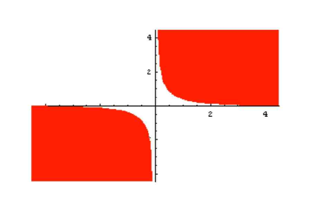
We have derived the result (3.35) for the boundary energy under the assumption that the Bethe roots for the ground state have the form (3.14), which is true only for suitable values of the boundary parameters $\beta_{\pm}$. For example, the shaded region in Fig. 1 denotes the region of parameter space for which the ground-state Bethe roots have the form (3.14) for $p=4$ and $N=2$. For parameter values outside the shaded region, one or more of the Bethe roots has an imaginary part which is not a multiple of $\pi/2$ and which evidently depends on the parameter values (but in a manner which we have not yet explicitly determined). As $p$ increases, the figure is similar, except that the shaded region moves further away from the origin.

Figure 1: Shaded region denotes region of the $(\beta_{+}\,,\beta_{-})$ plane for which the ground-state Bethe roots have the form (3.14) for $p=4$ and $N=2$.

A qualitative explanation of these features can be deduced from a short heuristic argument. Indeed, let us rewrite the Hamiltonian (3.1) as

$${\mathcal{H}}={\mathcal{H}}_{0}+h^{z}_{1}\sigma_{1}^{z}+h^{x}_{1}\sigma_{1}^{x}+h^{z}_{N}\sigma_{N}^{z}+h^{x}_{N}\sigma_{N}^{x}\,,$$ (3.36)

where the boundary magnetic fields are given by

$$h^{z}_{1} = {1\over 2}\mathop{\rm cosh}\nolimits\eta\mathop{\rm tanh}\nolimits\beta_{-}\,,\quad h^{x}_{1}={1\over 2}\mathop{\rm sech}\nolimits\beta_{-}$$

$$h^{z}_{N} = -{1\over 2}\mathop{\rm cosh}\nolimits\eta\mathop{\rm tanh}\nolimits\beta_{+}\,,\quad h^{x}_{N}={1\over 2}\mathop{\rm sech}\nolimits\beta_{+}\,.$$ (3.37)

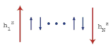
For $\beta_{+}\beta_{-}>\!\!>0$ (i.e., the shaded regions in Fig. 1), the boundary fields in the $x$ direction are small; moreover, $h^{z}_{1}h^{z}_{N}<0$; i.e., the boundary fields in the $z$ direction have antiparallel orientations, which (since $N$ is even) is compatible with a Néel-like (antiferromagnetic) alignment of the spins. (See Fig. 2.) Hence, the ground state and corresponding Bethe roots are “simple”.

Figure 2: Antiparallel boundary fields (big, red) are compatible with antiferromagnetic alignment of spins (small, blue)

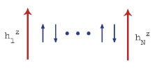
On the other hand, if $|\beta_{\pm}|$ are small (the unshaded region near the origin of Fig. 1), then the boundary fields in the $x$ direction are large. Also, if $\beta_{+}\beta_{-}<0$ (the second and fourth quadrants of Fig.1, which are also unshaded), then $h^{z}_{1}h^{z}_{N}>0$; i.e., the boundary fields in the $z$ direction are parallel, which can lead to “frustration”. (See Fig. 3.) For these cases, the ground states and corresponding Bethe roots are “complicated”.

Figure 3: Parallel boundary fields (big, red) are not compatible with antiferromagnetic alignment of spins (small, blue)

4 Case II: $p$ odd

For Case II (1.7), the Hamiltonian (1.1) becomes

$${\mathcal{H}}={\mathcal{H}}_{0}+{1\over 2}\mathop{\rm sinh}\nolimits\eta\left(\mathop{\rm cosech}\nolimits\alpha_{-}\sigma_{1}^{x}+\mathop{\rm cosech}\nolimits\alpha_{+}\sigma_{N}^{x}\right)\,.$$ (4.1)

We restrict $\alpha_{\pm}$ to be purely imaginary in order for the Hamiltonian to be Hermitian. We use the periodicity $\alpha_{\pm}\mapsto\alpha_{\pm}+2\pi i$ of the transfer matrix to further restrict $\alpha_{\pm}$ to the fundamental domain $-\pi\leq\Im m\ \alpha_{\pm}<\pi$. The eigenvalues $\Lambda(u)$ of the transfer matrix (2.1) are given by [15]

$$\Lambda(u) = {\delta(u-\eta)\over h^{(2)}(u-\eta)}{Q_{2}(u-\eta)\over Q_{1}(u)}+{\delta(u)\over h^{(1)}(u)}{Q_{2}(u+\eta)\over Q_{1}(u)}\,,$$ (4.2)

$$= h^{(1)}(u-\eta){Q_{1}(u-\eta)\over Q_{2}(u)}+h^{(2)}(u){Q_{1}(u+\eta)\over Q_{2}(u)}\,,$$

where

$$h^{(1)}(u) = {8\sinh^{2N+1}(u+2\eta)\cosh^{2}(u+\eta)\cosh(u+2\eta)\over\sinh(2u+3\eta)}\,,\quad h^{(2)}(u)=h^{(1)}(-u-2\eta)\,,$$ (4.3)

$$\delta(u) = h^{(1)}(u)h^{(2)}(u)\sinh(u+\eta+\alpha_{-})\sinh(u+\eta-\alpha_{-})\sinh(u+\eta+\alpha_{+})\sinh(u+\eta-\alpha_{+})\,,$$

and

$$Q_{a}(u)=\prod_{j=1}^{M_{a}}\sinh(u-u_{j}^{(a)})\sinh(u+u_{j}^{(a)}+\eta)\,,\qquad a=1\,,2\,,$$ (4.4)

with

$$M_{1}={1\over 2}(N+p+1)\,,\qquad M_{2}={1\over 2}(N+p-1)\,.$$ (4.5)

As remarked in the Introduction, the expressions for the eigenvalues (4.2) correspond to generalized $T-Q$ relations (1.4). For generic values of $\alpha_{\pm}$, we have not managed to reformulate this solution in terms of a single $Q(u)$. The zeros $\{u_{j}^{(a)}\}$ of $Q_{a}(u)$ are given by the Bethe Ansatz equations,

$${\delta(u_{j}^{(1)})\ h^{(2)}(u_{j}^{(1)}-\eta)\over\delta(u_{j}^{(1)}-\eta)\ h^{(1)}(u_{j}^{(1)})} = -{Q_{2}(u_{j}^{(1)}-\eta)\over Q_{2}(u_{j}^{(1)}+\eta)}\,,\qquad j=1\,,2\,,\ldots\,,M_{1}\,,$$

$${h^{(1)}(u_{j}^{(2)}-\eta)\over h^{(2)}(u_{j}^{(2)})} = -{Q_{1}(u_{j}^{(2)}+\eta)\over Q_{1}(u_{j}^{(2)}-\eta)}\,,\qquad j=1\,,2\,,\ldots\,,M_{2}\,.$$ (4.6)

In terms of the “shifted” Bethe roots $\tilde{u}_{j}^{(a)}\equiv u_{j}^{(a)}+{\eta\over 2}$, the Bethe Ansatz equations are

$$\left({\sinh(\tilde{u}_{j}^{(1)}+{\eta\over 2})\over\sinh(\tilde{u}_{j}^{(1)}-{\eta\over 2})}\right)^{2N+1}{\cosh(\tilde{u}_{j}^{(1)}-{\eta\over 2})\over\cosh(\tilde{u}_{j}^{(1)}+{\eta\over 2})}$$ (4.7)

$$\times{\sinh(\tilde{u}_{j}^{(1)}+\alpha_{-}-{\eta\over 2})\over\sinh(\tilde{u}_{j}^{(1)}-\alpha_{-}+{\eta\over 2})}{\sinh(\tilde{u}_{j}^{(1)}-\alpha_{-}-{\eta\over 2})\over\sinh(\tilde{u}_{j}^{(1)}+\alpha_{-}+{\eta\over 2})}{\sinh(\tilde{u}_{j}^{(1)}+\alpha_{+}-{\eta\over 2})\over\sinh(\tilde{u}_{j}^{(1)}-\alpha_{+}+{\eta\over 2})}{\sinh(\tilde{u}_{j}^{(1)}-\alpha_{+}-{\eta\over 2})\over\sinh(\tilde{u}_{j}^{(1)}+\alpha_{+}+{\eta\over 2})}$$

$$=-\prod_{k=1}^{M_{2}}{\sinh(\tilde{u}_{j}^{(1)}-\tilde{u}_{k}^{(2)}+\eta)\over\sinh(\tilde{u}_{j}^{(1)}-\tilde{u}_{k}^{(2)}-\eta)}{\sinh(\tilde{u}_{j}^{(1)}+\tilde{u}_{k}^{(2)}+\eta)\over\sinh(\tilde{u}_{j}^{(1)}+\tilde{u}_{k}^{(2)}-\eta)}\,,\quad j=1\,,\cdots\,,M_{1}\,.$$

and

$$\left({\sinh(\tilde{u}_{j}^{(2)}+{\eta\over 2})\over\sinh(\tilde{u}_{j}^{(2)}-{\eta\over 2})}\right)^{2N+1}{\cosh(\tilde{u}_{j}^{(2)}-{\eta\over 2})\over\cosh(\tilde{u}_{j}^{(2)}+{\eta\over 2})}$$ (4.8)

$$=-\prod_{k=1}^{M_{1}}{\sinh(\tilde{u}_{j}^{(2)}-\tilde{u}_{k}^{(1)}+\eta)\over\sinh(\tilde{u}_{j}^{(2)}-\tilde{u}_{k}^{(1)}-\eta)}{\sinh(\tilde{u}_{j}^{(2)}+\tilde{u}_{k}^{(1)}+\eta)\over\sinh(\tilde{u}_{j}^{(2)}+\tilde{u}_{k}^{(1)}-\eta)}\,,\quad j=1\,,\cdots\,,M_{2}\,.$$

The energy is given by

$$E={1\over 2}\sinh^{2}\eta\sum_{a=1}^{2}\sum_{j=1}^{M_{a}}{1\over\sinh(\tilde{u}_{j}^{(a)}-{\eta\over 2})\sinh(\tilde{u}_{j}^{(a)}+{\eta\over 2})}+{1\over 2}(N-1)\cosh\eta\,.$$ (4.9)

Indeed, for $p>1$, we obtain this result by following steps similar to those leading to (3.9). For $p=1$, we use (2.13) and (2.14) instead of (2.10) and (2.11); nevertheless, the result (4.9) holds also for $p=1$.

From numerical studies for small values of $N$ and $p$, and for suitable values of the boundary parameters $\alpha_{\pm}$ (which we discuss after Eq. (4.32) below), we find that the ground state is described by Bethe roots $\{\tilde{u}_{j}^{(1)}\}$ and $\{\tilde{u}_{j}^{(2)}\}$ of the form

$$\left\{\begin{array}[]{c@{\quad: \quad} l}v_{j}^{(1,1)}&j=1\,,2\,,\ldots\,,{N\over 2}\\ v_{j}^{(1,2)}+{i\pi\over 2}\,,&j=1\,,2\,,\ldots\,,{p+1\over 2}\end{array}\right.\,,\qquad\left\{\begin{array}[]{c@{\quad: \quad} l}v_{j}^{(2,1)}&j=1\,,2\,,\ldots\,,{N\over 2}\\ v_{j}^{(2,2)}+{i\pi\over 2}\,,&j=1\,,2\,,\ldots\,,{p-1\over 2}\end{array}\right.\,,$$ (4.14)

respectively, where $\{v_{j}^{(a,b)}\}$ are all real and positive.

We make the “string hypothesis” that (4.14) remains true in the thermodynamic limit ($N\rightarrow\infty$ with $p$ fixed). That is, that the Bethe roots $\{\tilde{u}_{j}^{(a)}\}$ for the ground state have the form

$$\left\{\begin{array}[]{c@{\quad: \quad} l}v_{j}^{(a,1)}&j=1\,,2\,,\ldots\,,M_{(a,1)}\\ v_{j}^{(a,2)}+{i\pi\over 2}\,,&j=1\,,2\,,\ldots\,,M_{(a,2)}\end{array}\right.\,,\qquad a=1\,,2\,,$$ (4.17)

where $\{v_{j}^{(a,b)}\}$ are all real and positive; also, $M_{(1,1)}=M_{(2,1)}={N\over 2}$, and $M_{(1,2)}={p+1\over 2}$, $M_{(2,2)}={p-1\over 2}$. Evidently there are two “seas” of real roots, namely $\{v_{j}^{(1,1)}\}$ and $\{v_{j}^{(2,1)}\}$.

We now proceed to compute the boundary energy, using notations similar to those in Case I. Defining

$$v_{j}^{(a,b)}=\mu\lambda_{j}^{(a,b)}\,,$$ (4.18)

the Bethe Ansatz equations (4.7), (4.8) for the sea roots are

$$e_{1}(\lambda_{j}^{(1,1)})^{2N+1}\left[g_{1}(\lambda_{j}^{(1,1)})e_{1+2a_{-}}(\lambda_{j}^{(1,1)})e_{1-2a_{-}}(\lambda_{j}^{(1,1)})e_{1+2a_{+}}(\lambda_{j}^{(1,1)})e_{1-2a_{+}}(\lambda_{j}^{(1,1)})\right]^{-1}$$

$$=-\prod_{k=1}^{N/2}\left[e_{2}(\lambda_{j}^{(1,1)}-\lambda_{k}^{(2,1)})e_{2}(\lambda_{j}^{(1,1)}+\lambda_{k}^{(2,1)})\right]\prod_{k=1}^{(p-1)/2}\left[g_{2}(\lambda_{j}^{(1,1)}-\lambda_{k}^{(2,2)})g_{2}(\lambda_{j}^{(1,1)}+\lambda_{k}^{(2,2)})\right]\,,$$

and

$$e_{1}(\lambda_{j}^{(2,1)})^{2N+1}g_{1}(\lambda_{j}^{(2,1)})^{-1}$$

$$=-\prod_{k=1}^{N/2}\left[e_{2}(\lambda_{j}^{(2,1)}-\lambda_{k}^{(1,1)})e_{2}(\lambda_{j}^{(2,1)}+\lambda_{k}^{(1,1)})\right]\prod_{k=1}^{(p+1)/2}\left[g_{2}(\lambda_{j}^{(2,1)}-\lambda_{k}^{(1,2)})g_{2}(\lambda_{j}^{(2,1)}+\lambda_{k}^{(1,2)})\right]\,,$$

respectively, where $j=1\,,\ldots\,,{N\over 2}$. The corresponding ground-state counting functions are

$$\mathsf{h}^{(1)}(\lambda)={1\over 2\pi}\Big{\{}(2N+1)q_{1}(\lambda)-r_{1}(\lambda)-q_{1+2a_{-}}(\lambda)-q_{1-2a_{-}}(\lambda)-q_{1+2a_{+}}(\lambda)-q_{1-2a_{+}}(\lambda)$$ (4.21)

$$-\sum_{k=1}^{N/2}\left[q_{2}(\lambda-\lambda_{k}^{(2,1)})+q_{2}(\lambda+\lambda_{k}^{(2,1)})\right]-\sum_{k=1}^{(p-1)/2}\left[r_{2}(\lambda-\lambda_{k}^{(2,2)})+r_{2}(\lambda+\lambda_{k}^{(2,2)})\right]\Big{\}}\,,$$

and

$$\mathsf{h}^{(2)}(\lambda)={1\over 2\pi}\Big{\{}(2N+1)q_{1}(\lambda)-r_{1}(\lambda)$$ (4.22)

$$-\sum_{k=1}^{N/2}\left[q_{2}(\lambda-\lambda_{k}^{(1,1)})+q_{2}(\lambda+\lambda_{k}^{(1,1)})\right]-\sum_{k=1}^{(p+1)/2}\left[r_{2}(\lambda-\lambda_{k}^{(1,2)})+r_{2}(\lambda+\lambda_{k}^{(1,2)})\right]\Big{\}}\,.$$

Repeating the maneuver (3.20) in the summations over the sea roots, and letting $N$ become large, we obtain a pair of coupled linear integral equations for the ground-state root densities $\rho^{(a)}(\lambda)$,

$$\rho^{(1)}(\lambda) = {1\over N}{d\mathsf{h}^{(1)}\over d\lambda}=2a_{1}(\lambda)-\int_{-\infty}^{\infty}d\lambda^{\prime}\ a_{2}(\lambda-\lambda^{\prime})\ \rho^{(2)}(\lambda^{\prime})$$ (4.23)

$$+ {1\over N}\Big{\{}a_{1}(\lambda)+a_{2}(\lambda)-b_{1}(\lambda)-a_{1+2a_{-}}(\lambda)-a_{1-2a_{-}}(\lambda)$$

$$- a_{1+2a_{+}}(\lambda)-a_{1-2a_{+}}(\lambda)-\sum_{k=1}^{(p-1)/2}\left[b_{2}(\lambda-\lambda_{k}^{(2,2)})+b_{2}(\lambda+\lambda_{k}^{(2,2)})\right]\Big{\}}\,,$$

and

$$\rho^{(2)}(\lambda) = {1\over N}{d\mathsf{h}^{(2)}\over d\lambda}=2a_{1}(\lambda)-\int_{-\infty}^{\infty}d\lambda^{\prime}\ a_{2}(\lambda-\lambda^{\prime})\ \rho^{(1)}(\lambda^{\prime})$$ (4.24)

$$+ {1\over N}\Big{\{}a_{1}(\lambda)+a_{2}(\lambda)-b_{1}(\lambda)-\sum_{k=1}^{(p+1)/2}\left[b_{2}(\lambda-\lambda_{k}^{(1,2)})+b_{2}(\lambda+\lambda_{k}^{(1,2)})\right]\Big{\}}\,.$$

It is straightforward to solve by Fourier transforms for the individual root densities. However, we shall see that the energy depends only on the sum of the root densities, which is given by

$$\rho^{(1)}(\lambda)+\rho^{(2)}(\lambda)=4s(\lambda)+{1\over N}{\cal R}(\lambda)\,,$$ (4.25)

where

$$\hat{\cal R}(\omega)= = {1\over 1+\hat{a}_{2}(\omega)}\Big{\{}2\hat{a}_{1}(\omega)+2\hat{a}_{2}(\omega)-2\hat{b}_{1}(\omega)-\hat{a}_{1+2a_{-}}(\omega)-\hat{a}_{1-2a_{-}}(\omega)$$ (4.26)

$$- \hat{a}_{1+2a_{+}}(\omega)-\hat{a}_{1-2a_{+}}(\omega)-2\sum_{a=1}^{2}\sum_{k=1}^{M_{(a,2)}}\cos(\omega\lambda_{k}^{(a,2)})\ \hat{b}_{2}(\omega)\Big{\}}\,.$$

The expression (4.9) for the energy and the string hypothesis (4.14) imply

$$E = -{1\over 2}\sinh^{2}\eta\Big{\{}-\sum_{a=1}^{2}\sum_{j=1}^{N/2}{1\over\sinh(v_{j}^{(a,1)}-{\eta\over 2})\sinh(v_{j}^{(a,1)}+{\eta\over 2})}$$ (4.27)

$$-\sum_{a=1}^{2}\sum_{j=1}^{M_{(a,2)}}{1\over\cosh(v_{j}^{(a,2)}-{\eta\over 2})\cosh(v_{j}^{(a,2)}+{\eta\over 2})}\Big{\}}+{1\over 2}(N-1)\cosh\eta$$

$$= -{\pi\sin\mu\over\mu}\Big{\{}\sum_{a=1}^{2}\sum_{j=1}^{N/2}a_{1}(\lambda_{j}^{(a,1)})+\sum_{a=1}^{2}\sum_{j=1}^{M_{(a,2)}}b_{1}(\lambda_{j}^{(a,2)})\Big{\}}+{1\over 2}(N-1)\cos\mu$$

$$= -{\pi\sin\mu\over\mu}\Big{\{}{1\over 2}\sum_{a=1}^{2}\sum_{j=-N/2}^{N/2}a_{1}(\lambda_{j}^{(a,1)})-a_{1}(0)+\sum_{a=1}^{2}\sum_{j=1}^{M_{(a,2)}}b_{1}(\lambda_{j}^{(a,2)})\Big{\}}+{1\over 2}(N-1)\cos\mu$$

$$= -{\pi\sin\mu\over\mu}\Big{\{}{N\over 2}\int_{-\infty}^{\infty}d\lambda\ a_{1}(\lambda)\left[\rho^{(1)}(\lambda)+\rho^{(2)}(\lambda)\right]-a_{1}(0)$$

$$+\sum_{a=1}^{2}\sum_{j=1}^{M_{(a,2)}}b_{1}(\lambda_{j}^{(a,2)})\Big{\}}+{1\over 2}(N-1)\cos\mu\,.$$

Substituting the result (4.25) for the sum of the root densities, we obtain

$$E=E_{bulk}+E_{boundary}\,,$$ (4.28)

where the bulk (order $N$) energy is again given by (3.32), and the boundary (order $1$) energy is given by

$$E_{boundary}=-{\pi\sin\mu\over\mu}\Big{\{}{\cal I}+\sum_{a=1}^{2}\sum_{j=1}^{M_{(a,2)}}b_{1}(\lambda_{j}^{(a,2)})\Big{\}}-{1\over 2}\cos\mu\,,$$ (4.29)

where ${\cal I}$ is the integral

$${\cal I} = {1\over 2}\int_{-\infty}^{\infty}d\lambda\ a_{1}(\lambda)\left[{\cal R}(\lambda)-2\delta(\lambda)\right]={1\over 4\pi}\int_{-\infty}^{\infty}d\omega\ \hat{a}_{1}(\omega)\left[\hat{\cal R}(\omega)-2\right]$$ (4.30)

$$= -\sum_{a=1}^{2}\sum_{j=1}^{M_{(a,2)}}b_{1}(\lambda_{j}^{(a,2)})+{1\over 2\pi}\int_{-\infty}^{\infty}d\omega\ \hat{s}(\omega)\Big{\{}\hat{a}_{1}(\omega)-\hat{b}_{1}(\omega)-1$$

$$-{1\over 2}\left[\hat{a}_{1+2a_{-}}(\omega)+\hat{a}_{1-2a_{-}}(\omega)+\hat{a}_{1+2a_{+}}(\omega)+\hat{a}_{1-2a_{+}}(\omega)\right]\Big{\}}\,.$$

Once again there is a remarkable cancellation among terms involving Bethe roots which are not parts of the seas, namely, $\lambda_{j}^{(a,2)}$. Writing $E_{boundary}$ as the sum of contributions from the left and right boundaries, we conclude that for the parameter values

$${1\over 2}\leq|a_{\pm}|<\nu-{1\over 2}\,,$$ (4.31)

the energy contribution from each boundary is given by

$$E_{boundary}^{\pm} = -{\sin\mu\over 2\mu}\int_{-\infty}^{\infty}d\omega\ {1\over 2\cosh(\omega/2)}\Big{\{}{\cosh((\nu-2)\omega/4)\over 2\cosh(\nu\omega/4)}-{1\over 2}$$ (4.32)

$$+ {\sinh(\omega/2)\cosh((\nu-2|a_{\pm}|)\omega/2)\over\sinh(\nu\omega/2)}\Big{\}}-{1\over 4}\cos\mu\,.$$

This result agrees with the result (1.8) with $b_{\pm}=0$ and $a_{\pm}$ values (4.31). As shown in the Appendix, the integrals (with $p$ odd) can also be evaluated analytically.

We have derived the above result for the boundary energy under the assumption that the Bethe roots for the ground state have the form (4.14), which is true only for suitable values of the boundary parameters $a_{\pm}$, namely,

$${\nu-1\over 2}<|a_{\pm}|<{\nu+1\over 2}\,,\qquad a_{+}a_{-}>0\,,$$ (4.33)

where $\nu=p+1$. For parameter values outside the region (4.33), one or more of the Bethe roots has an imaginary part which is not a multiple of $\pi/2$ and which evidently depends on the parameter values. One can verify that the region (4.33) is contained in the region (4.31).

As in Case I, it is possible to give a qualitative explanation of the restriction (4.33) by a heuristic argument. Indeed, let us rewrite the Hamiltonian (4.1) as

$${\mathcal{H}}={\mathcal{H}}_{0}+h^{x}_{1}\sigma_{1}^{x}+h^{x}_{N}\sigma_{N}^{x}\,,$$ (4.34)

where the boundary magnetic fields are given by

$$h^{x}_{1}={1\over 2}\sinh\eta\mathop{\rm cosech}\nolimits\alpha_{-}\,,\quad h^{x}_{N}={1\over 2}\sinh\eta\mathop{\rm cosech}\nolimits\alpha_{+}\,.$$ (4.35)

For $\alpha_{\pm}\approx i\pi/2$ or $-i\pi/2$ (i.e., $a_{\pm}\approx\nu/2$ or $-\nu/2$), the boundary magnetic fields in the $x$ direction are small and parallel. Hence, the ground state and corresponding Bethe roots are “simple”. Outside of this region of parameter space, the boundary fields in the $x$ direction are large and/or antiparallel, and so the ground state and corresponding Bethe roots are “complicated”.

5 Discussion

We have investigated the ground state of the open XXZ spin chain with nondiagonal boundary terms which are parametrized by pairs of boundary parameters, in the thermodynamic limit, using the new exact solutions [14, 15] and the string hypothesis. This investigation has revealed some surprises. Indeed, for Case I (1.6), the ground state is described in part by a sea of strings of length 2 (3.14), which is characteristic of spin-1 chains [20]. For Case II (1.7), the energy depends on two sets of Bethe roots (4.9), and in fact on the sum of the corresponding root densities (4.27). For each case, there is a remarkable cancellation of the energy contributions from non-sea Bethe roots.

Perhaps the biggest surprise is that, for the two cases studied here, the boundary energies coincide with the result (1.8) for the constrained case (1.3), even when that constraint is not satisfied. This suggests that the result (1.8) may hold for general values of the boundary parameters. A first step toward checking this conjecture would be to extend our analysis to the “unshaded” regions of parameter space, where the ground state has Bethe roots whose imaginary parts depend on the parameters.

We have not computed the Casimir (order $1/N$) energy for the two cases (1.6), (1.7). The computation should be particularly challenging for the former case, due to the presence of a complex sea. It would be interesting to investigate excited states, and also applications to other problems, including the boundary sine-Gordon model. We hope to be able to address such questions in the future.

Appendix A Appendix

Here we present more explicit expressions for the bulk and boundary energies.

A.1 Case I: $p$ even

The integral appearing in the bulk energy (3.32) for $p$ even is given by

$$I_{1} \equiv \int_{-\infty}^{\infty}d\lambda\ a_{1}(\lambda)\ s(\lambda)={1\over 2\pi}\int_{-\infty}^{\infty}d\omega\ \hat{a}_{1}(\omega)\ \hat{s}(\omega)$$ (A.1)

$$= {\mu\over\pi}\sum_{j=1}^{p\over 2}(-1)^{j+{p\over 2}}\tan\Big{(}\big{(}j-{1\over 2}\big{)}\mu\Big{)}\,.$$

The parameter-dependent integral appearing in the boundary energy (3.35) is given by

$$I_{2}(x) \equiv {1\over 2\pi}\int_{-\infty}^{\infty}d\omega\ {\sinh(\omega/2)\cos(x\omega)\over 2\sinh(\nu\omega/2)\cosh(\omega/2)}$$ (A.2)

$$= \sum_{j=1}^{p\over 2}(-1)^{j+{p\over 2}}b_{j-{1\over 2}}(x/2)-{1\over 2}b_{p+1\over 2}(x/2)\,,$$

where the function $b_{n}(\lambda)$ is defined in (3.23). Moreover,

$${1\over 2\pi}\int_{-\infty}^{\infty}d\omega\ {\sinh(\omega/2)\cosh((\nu-2)\omega/2)\over 2\sinh(\nu\omega/2)\cosh(\omega/2)}=I_{2}(i(p-1)/2)\,,$$ (A.3)

and

$${1\over 2\pi}\int_{-\infty}^{\infty}d\omega\ {\sinh((\nu-2)\omega/4)\over 4\sinh(\nu\omega/4)\cosh(\omega/2)}={1\over 2}\left[I_{1}-I_{2}(0)\right]\,.$$ (A.4)

It follows that the boundary energy (3.35) is given by

$$E_{boundary}^{\pm}=-{\pi\sin\mu\over\mu}\Big{\{}{1\over 2}I_{1}-{1\over 2}I_{2}(0)+I_{2}(i(p-1)/2)+I_{2}(b_{\pm})-{1\over 4}\Big{\}}-{1\over 4}\cos\mu\,,$$ (A.5)

where $I_{1}$ and $I_{2}(x)$ are given by (A.1) and (A.2), respectively.

A.2 Case II: $p$ odd

The integral appearing in the bulk energy (3.32) for $p$ odd is given by

$$I_{1} \equiv \int_{-\infty}^{\infty}d\lambda\ a_{1}(\lambda)\ s(\lambda)={1\over 2\pi}\int_{-\infty}^{\infty}d\omega\ \hat{a}_{1}(\omega)\ \hat{s}(\omega)$$ (A.6)

$$= {\mu\over\pi^{2}}\Big{[}1+2\mu\sum_{j=1}^{p-1\over 2}j\cot(j\mu)\Big{]}\,.$$

The parameter-dependent integral appearing in the boundary energy (4.32) is given by

$$I_{2}(x) \equiv {1\over 2\pi}\int_{-\infty}^{\infty}d\omega\ {\sinh(\omega/2)\cosh(x\omega)\over 2\sinh(\nu\omega/2)\cosh(\omega/2)}$$ (A.7)

$$= {(-1)^{p-1\over 2}\mu\over\pi\sin(x\pi)}\left[x+\sum_{j=1}^{p-1\over 2}(-1)^{j}\cot(j\mu)\sin(2xj\mu)\right]\,.$$

Moreover,

$${1\over 2\pi}\int_{-\infty}^{\infty}d\omega\ {\cosh((\nu-2)\omega/4)\over 4\cosh(\nu\omega/4)\cosh(\omega/2)}={1\over 2}\left[I_{1}+I_{2}(0)\right]\,.$$ (A.8)

It follows that the boundary energy (4.32) is given by

$$E_{boundary}^{\pm}=-{\pi\sin\mu\over\mu}\Big{\{}{1\over 2}I_{1}+{1\over 2}I_{2}(0)+I_{2}((p+1-2|a_{\pm}|)/2)-{1\over 4}\Big{\}}-{1\over 4}\cos\mu\,,$$ (A.9)

where $I_{1}$ and $I_{2}(x)$ are given by (A.6) and (A.7), respectively.

References

[1]
M. Gaudin,
Phys. Rev.A4, 386 (1971); La fonction d’onde de
Bethe (Masson, 1983).
[2]
F.C. Alcaraz, M.N. Barber, M.T. Batchelor, R.J. Baxter and G.R.W. Quispel,
J. Phys.A20, 6397 (1987).
[3]
E.K. Sklyanin,
J. Phys.A21, 2375 (1988).
[4]
H.J. de Vega and A. González-Ruiz,
J. Phys.A26, L519 (1993)
[hep-th/9211114]
[5]
S. Ghoshal and A. B. Zamolodchikov,
Int. J. Mod. Phys.A9, 3841 (1994)
[hep-th/9306002]
[6]
J. Cao, H.-Q. Lin, K.-J. Shi and Y. Wang,
[cond-mat/0212163]; Nucl. Phys.B663, 487 (2003).
[7]
R.I. Nepomechie,
J. Stat. Phys.111, 1363 (2003)
[hep-th/0211001];
J. Phys.A37, 433 (2004)
[hep-th/0304092]
[8]
R.I. Nepomechie and F. Ravanini,
J. Phys.A36, 11391 (2003);
Addendum, J. Phys.A37, 1945 (2004)
[hep-th/0307095]
[9]
W.-L. Yang, R.I. Nepomechie and Y.-Z. Zhang,
[hep-th/0511134]
[10]
C. Ahn and R.I. Nepomechie,
Nucl. Phys.B676, 637 (2004)
[hep-th/0309261];
[11]
C. Ahn, Z. Bajnok, R.I. Nepomechie, L. Palla and G. Takács,
Nucl. Phys.B714, 307 (2005)
[hep-th/0501047]
[12]
J.-S. Caux, H. Saleur and F. Siano,
Phys. Rev. Lett.88, 106402 (2002)
[hep-th/0109103];
Nucl. Phys.B672, 411 (2003)
[hep-th/0306328];
T. Lee and C. Rim,
Nucl. Phys.B672, 487 (2003)
[hep-th/0301075]
[13]
A. Doikou,
Nucl. Phys.B668, 447 (2003)
[hep-th/0303205];
J. de Gier and P. Pyatov,
J. Stat. Mech.P03002 (2004)
[hep-th/0312235];
W. Galleas and M.J. Martins,
Phys. Lett.A335, 167 (2005)
[nlin.SI/0407027];
C.S. Melo, G.A.P. Ribeiro and M.J. Martins,
Nucl. Phys.B711, 565 (2005)
[nlin.SI/0411038];
W.-L. Yang, Y.-Z. Zhang and M. Gould,
Nucl. Phys.B698, 503 (2004)
[hep-th/0411048];
W.-L. Yang and Y.-Z. Zhang,
JHEP0501, 021 (2005)
[hep-th/0411190];
W.-L. Yang, Y.-Z. Zhang and R. Sasaki,
Nucl. Phys.B729, 594 (2005)
[hep-th/0507148];
J. de Gier, A. Nichols, P. Pyatov and V. Rittenberg,
Nucl. Phys.B729, 387 (2005)
[hep-th/0505062];
J. de Gier and F.H.L. Essler,
[cond-mat/0508707]
[14]
R. Murgan and R.I. Nepomechie,
J. Stat. Mech.P05007 (2005);
Addendum, J. Stat. Mech.P11004 (2005)
[hep-th/0504124]
[15]
J. Stat. Mech.P08002 (2005)
[hep-th/0507139]