Graviton and Spherical Graviton Potentials
in Plane-Wave Matrix Model
  - overview and perspective -

KEK-TH-1053

hep-th/0511187

H. Shin and K. YoshidaGraviton and Giant Graviton Potentials in Plane-Wave Matrix Model

1, Hyeonjoon Shin2

1

2

We briefly review our works for graviton and spherical graviton potentials in a plane-wave matrix model. To compute them, it is necessary to devise a configuration of the graviton solutions, since the plane-wave matrix model includes mass terms and hence the gravitons are not free particles as in the BFSS matrix model but harmonic oscillators or rotating particles. The configuration we proposed consists of a rotating graviton and an elliptically rotating graviton. It is applied to the two-body interaction of spherical gravitons in the $SO(6)$ symmetric space, and then to that of point-like gravitons in the $SO(3)$ symmetric space. In both cases the leading term of the resulting potential is $1/r^{7}$. This result strongly suggests that the potentials should be closely related to the light-front eleven-dimensional supergravity linearized around the pp-wave background.

1 Introduction

One of the most important problems in particle physics is to clarify the substance of M-theory which is believed as the unified theory of superstrings. Towards the formulation of M-theory, a matrix model approach gives a promising way. In fact, the matrix model proposed by Banks, Fischler, Shenker and Susskind (BFSS) is conjectured to describe a discrete light-cone quantized (light-front) M-theory [1]. It is basically a one-dimensional matrix quantum mechanics and called BFSS matrix model. It is closely related to a supermembrane theory in eleven dimensions via the matrix regularization [2].

M-theory is considered to contain the eleven-dimensional supergravity as a low energy effective theory. On the other hand, the matrix model is shown to contain the gravity and therefore this fact gives a strong evidence for the conjecture. More concretely speaking, graviton potentials in the light-front eleven-dimensional supergravity can be reproduced from the computation in the matrix model. For example, let us consider two graviton scattering in the BFSS matrix model. A single graviton is described by $1\times 1$ matrix,

$$X^{I}=a^{I}+v^{I}t\quad\mbox{(free~{}particle)}\,,$$ (1)

which is a classical solution. The configuration for two-graviton scattering is given by

$$B^{1}=\frac{1}{2}\begin{pmatrix}vt&0\\ 0&-vt\end{pmatrix}\,,\quad B^{2}=\frac{1}{2}\begin{pmatrix}b&0\\ 0&-b\end{pmatrix}\,,\quad B^{i}=0\quad(i>2)\,,$$ (2)

which is drawn in Fig. 1. By using the background field method and integrating out the fluctuations around the configuration (2), the potential is computed as a function of the impact parameter $b$ . The resulting potential is given by

$$V(b)=-\frac{15}{16}\frac{v^{4}}{b^{7}}+\mathcal{O}\left(\frac{v^{6}}{b^{11}}\right)\,.$$ (3)

The term proportional to $b$ and the lower order terms, that is, $1/b$ , $1/b^{3}$ and $1/b^{5}$, are canceled out basically because of supersymmetries. The term with $1/b^{9}$ also does not appear and hence the subleading term is $1/b^{11}$.

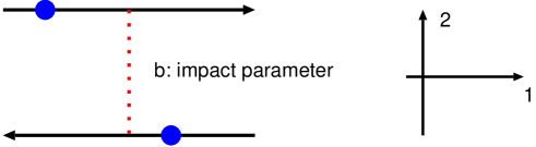
Figure 1: Two graviton scattering in the BFSS case

The one-loop result in the matrix model agrees with the potential derived by evaluating a tree diagram in the light-front eleven-dimensional supergravity, including the numerical factors. We would like to note that, in fact, the one-loop result has turned out to be exact entirely due to the power of 16 supersymmetries [3]. Spherical membrane scattering is also discussed in [4]. For the detail, see [5].

From now on, we will overview graviton and spherical graviton potentials in a plane-wave matrix model (PWMM) [6]. This matrix model may be considered as a generalization of the BFSS matrix model to the pp-wave background which has non-vanishing curvature. It is very interesting to consider whether the matrix model on the pp-wave background can describe the gravity correctly or not.

2 Plane-Wave Matrix Model

Here we shall briefly introduce a plane-wave matrix model. The action of the matrix model is given by [6]

$$S_{\rm pp}=\int\!\!dt\,\mathrm{Tr}\Bigl{[}\frac{1}{2R}D_{t}X^{I}D_{t}X^{I}+\frac{R}{4}([X^{I},X^{J}])^{2}+i\Theta^{\dagger}D_{t}\Theta-R\Theta^{\dagger}\gamma^{I}[\Theta,X^{I}]$$

$$\qquad\qquad-\frac{1}{2R}\left(\frac{\mu}{3}\right)^{2}(X^{i})^{2}-\frac{1}{2R}\left(\frac{\mu}{6}\right)^{2}(X^{a})^{2}-i\frac{\mu}{3}\epsilon^{ijk}X^{i}X^{j}X^{k}-i\frac{\mu}{4}\Theta^{\dagger}\gamma^{123}\Theta\Bigr{]}\,,$$ (4)

where the indices of the transverse nine-dimensional space are $I,J=1,\ldots,9$ and $R$ is the radius of the circle compactified along $x^{-}$ . All degrees of freedom are $N\times N$ Hermitian matrices and the covariant derivative $D_{t}$ with the gauge field $A$ is defined by $D_{t}=\partial_{t}-i[A,~{}~{}]$ . The plane-wave matrix model can be obtained from the supermembrane theory on the pp-wave background [7, 8] via the matrix regularization [2]. In particular, in the case of the pp-wave, the correspondence of superalgebra between the supermembrane theory and the matrix model, including brane charges, is established by the works [8] and [9].

This matrix model may be considered as a deformation of the BFSS matrix model while it still preserves linearly realized 16 supersymmetries. The plane-wave matrix model allows a static 1/2 BPS fuzzy sphere with zero light-cone energy to exist as a classical solution, since the action of the matrix model includes the Myers term [10]. The structure of the vacua is enriched with the fuzzy sphere. The spectra around the vacua are now fully clarified [7, 11]. The trivial vacuum $X^{I}=0$ has also been identified with a single spherical five-brane vacuum [12]. Except for the static fuzzy sphere,there are various classical solutions and those have been well studied (e.g., see [13]). BPS properties of fuzzy sphere have been investigated in several papers [7, 14, 15]. Thermal stabilities of classical solutions have also been investigated in [17].

Our purpose here is to compute the graviton potential in the plane-wave matrix model. One should note that the graviton solution (1) as a free particle is not a classical solution any more, since the plane-wave matrix model contains mass terms in contrast to the BFSS matrix model. The graviton solution in the plane-wave matrix model is represented by a harmonic oscillator or a rotating particle. Then it is necessary to devise the setup to examine the two-graviton scattering in the plane-wave matrix model. In the next section we will discuss the configuration of the gravitons for the computation of the potential. Before going to the explanation of the setup, in the next subsection we will explain the background field method and the exactness of the one-loop calculation in the $\mu\to\infty$ limit.

2.1 Background Field Method and One-Loop Exactness

To compute the interaction potential we use the background field method as usual. To begin with, the matrix variables are decomposed into the background and the fluctuations as

$$X^{I}=B^{I}+Y^{I}\,,\quad\Theta=0+\Psi\,.$$ (5)

where $B^{I}$ are the classical background fields while $Y^{I}$ and $\Psi$ are the quantum fluctuations around them. Here the fermionic background is set to zero.

In order to perform the path integration, we take the background field gauge which is usually chosen in the matrix model calculation as

$$D_{\mu}^{\rm bg}A^{\mu}_{\rm qu}\equiv D_{t}A+i[B^{I},X^{I}]=0~{}.$$ (6)

Then the corresponding gauge-fixing $S_{\mathrm{GF}}$ and Faddeev-Popov ghost $S_{\mathrm{FP}}$ terms are given by

$$S_{\mathrm{GF}}+S_{\mathrm{FP}}=\int\!dt\,{\rm Tr}\left(-\frac{1}{2}(D_{\mu}^{\rm bg}A^{\mu}_{\rm qu})^{2}-\bar{C}\partial_{t}D_{t}C+[B^{I},\bar{C}][X^{I},\,C]\right)\,.$$ (7)

Now by inserting the decomposition of the matrix fields (5) into the matrix model action, we get the gauge fixed plane-wave action $S$ $(\equiv S_{\rm pp}+S_{\mathrm{GF}}+S_{\mathrm{FP}})$ expanded around the background. The resulting action is read as $S=S_{0}+S_{2}+S_{3}+S_{4}$ , where $S_{n}$ represents the action of order $n$ with respect to the quantum fluctuations. Here we write down only the second order part:

$$S_{2}=\int\!\!dt\,\mathrm{Tr}\bigg{[}\,\frac{1}{2}(\dot{Y}^{I})^{2}-2i\dot{B}^{I}[A,\,Y^{I}]+[B^{I},\,B^{J}][Y^{I},\,Y^{J}]$$

$$+\frac{1}{2}([B^{I},\,Y^{J}])^{2}-i\mu\epsilon^{ijk}B^{i}Y^{j}Y^{k}-\frac{1}{2}\left(\frac{\mu}{3}\right)^{2}(Y^{i})^{2}-\frac{1}{2}\left(\frac{\mu}{6}\right)^{2}(Y^{a})^{2}$$

$$+i\Psi^{\dagger}\dot{\Psi}-\Psi^{\dagger}\gamma^{I}[\Psi,\,B^{I}]-i\frac{\mu}{4}\Psi^{\dagger}\gamma^{123}\Psi$$

$$-\frac{1}{2}\dot{A}^{2}-\frac{1}{2}([B^{I},\,A])^{2}+\dot{\bar{C}}\dot{C}+[B^{I},\,\bar{C}][B^{I},\,C]\,\bigg{]}\,.$$ (8)

The above expression is given in the Minkowski formulation and hereafter we will not move to the Euclidean formulation. The first order part $S_{1}$ vanishes by using the equation of motions. The zeroth order part is also zero for all of the classical configurations we consider later, although the solutions are rotating.

For the justification of one-loop computation or the semi-classical analysis, it should be made clear that $S_{3}$ and $S_{4}$ can be regarded as perturbations. For this purpose, following [7], we rescale the fluctuations and parameters as

$$A\rightarrow\mu^{-1/2}A~{},~{}~{}~{}Y^{I}\rightarrow\mu^{-1/2}Y^{I}~{},~{}~{}~{}C\rightarrow\mu^{-1/2}C~{},~{}~{}~{}t\rightarrow\mu^{-1}t~{}.$$ (9)

Under this rescaling, the action $S$ in the fuzzy sphere background becomes

$$S=S_{2}+\mu^{-3/2}S_{3}+\mu^{-3}S_{4}~{},$$ (10)

where the parameter $\mu$ in $S_{2}$, $S_{3}$ and $S_{4}$ has been replaced by 1 and so those do not have $\mu$ dependence. Now it is obvious that, in the large $\mu$ limit, $S_{3}$ and $S_{4}$ can be treated as perturbations and the one-loop computation gives the sensible result. Note that the analysis in the $S_{2}$ part is exact in the $\mu\rightarrow\infty$ limit. We can calculate the exact spectra around an $N$-dimensional irreducible fuzzy sphere in the $\mu\rightarrow\infty$ limit, by following the method in the work [7] (For the detail of the calculation, see [7, 15]). The exact spectra are useful to compute the giant graviton potential.

3 Giant Graviton Scattering

Here we consider a two-body scattering of spherical gravitons (fuzzy spheres) [15, 18] which expand in the $SO(3)$ symmetric space. These solutions are considered as giant gravitons. Hence we call the potential between the spherical gravitons the giant graviton potential.

3.1 One-Loop Flatness

As a first trial, we proposed a setup of the giant gravitons to compute the interaction potential, drawn in Fig. 2.

Two fuzzy spheres expand in the $SO(3)$ symmetric space, and in a sub-plane in the $SO(6)$ symmetric space a spherical membrane (with $p^{+}=N_{1}/R$) is sitting at the origin of the $SO(6)$ symmetric space and the other one (with $p^{+}=N_{2}/R$) rotates with $r$ .

The background is described as

$$B^{I}=\begin{pmatrix}B^{I}_{(1)}&0\\ 0&B^{I}_{(2)}\end{pmatrix},\quad\begin{array}[]{c}B^{I}_{(1)}:N_{1}\times N_{1}\\ B^{I}_{(2)}:N_{2}\times N_{2}\end{array},\quad N=N_{1}+N_{2}\vspace*{0.2cm}$$ (13)

$$B^{i}_{(s)}=\frac{\mu}{3}J^{i}_{(s)},\quad B^{6}_{(s)}=\dots=B^{9}_{(s)}=0\qquad(s=1,2)\,.$$

The rotation of the first fuzzy sphere is rotating around the origin with a constant radius $r$ ,

$$B^{4}_{(1)}=r\cos\left(\frac{\mu}{6}t\right){\bf 1}_{N_{1}\times N_{1}},\quad B^{5}_{(1)}=r\sin\left(\frac{\mu}{6}t\right){\bf 1}_{N_{1}\times N_{1}}\,,$$

and the second fuzzy sphere is sitting at the origin. When we rescale the variables as in (9) , the parameter $r$ is also rescaled as $r\to\mu r$ .

For this setup, we have computed the potential by integrating out the fluctuations around this background. The resulting potential is, however, zero and hence the system is shown to be BPS. Nevertheless, the system is still important as a start point since we can expect to obtain non-trivial potential by breaking the remaining supersymmetries. Thus the next task is to consider how to break the remaining supersymmetries.

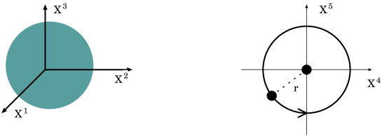
Figure 2: BPS configuration of two spherical gravitons in the PWMM case

3.2 Elliptic Deformation

In order to break the remaining supersymmetries, we hit on an elliptic deformation of the setup in Fig. 2. That is, we considered a configuration in a sub-plane in the $SO(6)$ symmetric space where a spherical membrane (with $p^{+}=N_{1}/R$) rotates with a constant radius $r_{1}$ and another one (with $p^{+}=N_{2}/R$) elliptically rotates with $r_{2}\pm\epsilon$ . The motion of the second fuzzy sphere is elliptically deformed with the infinitesimal parameter $\epsilon$ . This parameter plays the similar role with the velocity $v$ of the graviton in the BFSS case where $v$ is also assumed to be sufficiently small.

The motion of the first and the second fuzzy spheres are represented by, respectively,

$$B^{4}_{(1)}=r_{1}\cos\left(\frac{\mu}{6}t\right){\bf 1}_{N_{1}\times N_{1}},\quad B^{5}_{(1)}=r_{1}\sin\left(\frac{\mu}{6}t\right){\bf 1}_{N_{1}\times N_{1}}$$

$$B^{4}_{(2)}=(r_{2}+\epsilon)\cos\left(\frac{\mu}{6}t\right){\bf 1}_{N_{2}\times N_{2}},\quad B^{5}_{(2)}=(r_{2}-\epsilon)\sin\left(\frac{\mu}{6}t\right){\bf 1}_{N_{2}\times N_{2}}$$

The fuzzy spheres are expanding in the $SO(3)$ symmetric space. The parameters $r_{1,2}$ and $\epsilon$ are also rescaled as $r_{1,2}\,,~{}\epsilon\to\mu r_{1,2}\,,~{}\mu\epsilon$ .

For this setup we have computed the effective action by using the background field method. The resulting effective action with respect to $r\equiv r_{2}-r_{1}$ is

$$\Gamma_{\rm eff}=\epsilon^{4}\int\!\!dt\,\biggl{[}\frac{35}{2^{7}\cdot 3}\frac{N_{1}N_{2}}{r^{7}}-\frac{385}{2^{11}\cdot 3^{3}}\big{[}2(N_{1}^{2}+N_{2}^{2})-1\big{]}\frac{N_{1}N_{2}}{r^{9}}+\mathcal{O}\left(\frac{1}{r^{11}}\right)\biggr{]}+\mathcal{O}(\epsilon^{6})\,.$$ (14)

This result strongly suggests that the spherical membranes should be interpreted as spherical gravitons as discussed by Kabat and Taylor [4]. Here we should remark that the subleading term is $1/r^{9}$ and it is repulsive. In the BFSS case the subleading term is $1/r^{11}$ order and it implies the dipole-dipole interaction. According to the interpretation, the $1/r^{9}$ term would imply the dipole-graviton interaction. This is a new effect intrinsic to the pp-wave background.

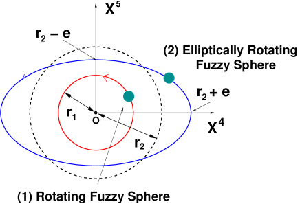
Figure 3: Scattering of two spherical gravitons in the PWMM case

4 Point-Like Graviton Scattering

Now we will discuss a two-body scattering in the $SO(3)$ symmetric space [19]. Then the configuration for the computation consists of two point-like gravitons in contrast to the spherical membrane cases, since fuzzy spheres cannot expand due to the directions of the constant flux. This background is represented by

$$B^{I}=\begin{pmatrix}B^{I}_{(1)}&0\\ 0&B^{I}_{(2)}\end{pmatrix}\qquad(I=1,\ldots,9)\,,$$

$$B^{1}_{(1)}=r_{1}\cos\left(\frac{\mu}{3}t\right)\,,\qquad B^{2}_{(1)}=r_{1}\sin\left(\frac{\mu}{3}t\right)\,,$$

$$B^{1}_{(2)}=(r_{2}+\epsilon)\cos\left(\frac{\mu}{3}t\right)\,,\qquad B^{2}_{(2)}=(r_{2}-\epsilon)\sin\left(\frac{\mu}{3}t\right)$$

$$B^{3}_{(s)}=B^{a}_{(s)}=0\qquad(s=1,2~{};~{}a=4,\ldots,9)\,.$$ (15)

In this setup two point-like gravitons are rotating in the 1-2 plane. One of them is rotating with a constant radius $r_{1}$ and the other is elliptically rotating with $r_{2}\pm\epsilon$ , as depicted in Fig. 4 .

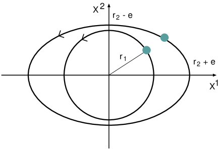
Figure 4: Two point-like gravitons in the PWMM case

We can compute the potential as a function of $r\equiv r_{2}-r_{1}$ , and the resulting potential is given by

$$\Gamma_{\rm eff} =\epsilon^{4}\int dt\left[~{}\frac{35}{24}\frac{1}{r^{7}}+\frac{385}{576}\frac{1}{r^{9}}+\mathcal{O}\left(\frac{1}{r^{11}}\right)~{}\right]+\mathcal{O}(\epsilon^{6})\,.$$

The leading term is also $1/r^{7}$ , but the subleading term is attractive in contrast to the spherical membrane cases. The numerical coefficients are also different from the case in the $SO(6)$ symmetric space, but it is not suspicious since the transverse $SO(9)$ symmetry is not preserved any more and it is broken to $SO(3)\times SO(6)$ .

5 Conclusion and Discussion

We have discussed two-body scatterings of gravitons and spherical gravitons in the plane-wave matrix model. The resulting potentials in both cases have $1/r^{7}$ term as the leading term. The $1/r^{7}$ behavior strongly suggests that the potentials should be related to the light-front eleven-dimensional supergravity. Eventually, it should be the linearized supergravity around the pp-wave background. It is an interesting direction to find the corresponding configuration in the supergravity side i.e., the tree diagram leading to the potential obtained in the matrix model computation. In the supergravity analysis it is necessary to take asymptotic states, but the spectrum of the linearized supergravity around the pp-wave background has already been obtained in [20]. By using this spectrum, it would be possible to rederive the potential from the supergravity, including the numerical coefficients as in the BFSS case. The work [21] would be helpful to study in this direction. We hope that we could report on the subject in another place in the near future.

It is worth noting again the subleading terms. The subleading term in the plane-wave matrix model case is $1/r^{9}$ in comparison to $1/r^{11}$ in the BFSS matrix model case. As for the signature of the term, it is repulsive in the $SO(6)$ case and attractive in the $SO(3)$ case. In the BFSS case the $1/r^{11}$ term is interpreted as a dipole-dipole interaction. According to an analogy to the BFSS case, the $1/r^{9}$ term should be interpreted as a graviton-dipole interaction. This term is intrinsic to the pp-wave background and may lead to some new physics. Thus it is valuable to clarify the meaning of the subleading term in connection with the geometry of the pp-wave background.

We hope that our potentials would be an important clue to clarify some features of M-theory on the pp-wave background, and furthermore that they shed light on M-theory on curved backgrounds.

References

- [1] T. Banks, W. Fischler, S. H. Shenker and L. Susskind, “M theory as a matrix model: A conjecture,” Phys. Rev. D55, 5112 (1997) 5112 [arXiv:hep-th/9610043].
- [2] B. de Wit, J. Hoppe and H. Nicolai, “On the quantum mechanics of supermembranes,” Nucl. Phys. B305, 545 (1988).
- [3] S. Paban, S. Sethi and M. Stern, “Constraints From Extended Supersymmetry in Quantum Mechanics,” Nucl. Phys. B534,137 (1998) [arXiv:hep-th/9805018]; S. Hyun, Y. Kiem and H. Shin, “Supersymmetric completion of supersymmetric quantum mechanics,” Nucl. Phys. B558, 349 (1999) [arXiv:hep-th/9903022].
- [4] D. Kabat and W. Taylor, “Spherical membranes in matrix theory,” Adv. Theor. Math. Phys. 2, 181 (1998) [arXiv:hep-th/9711078].
- [5] W. Taylor, “M(atrix) theory: Matrix quantum mechanics as a fundamental theory,” Rev. Mod. Phys. 73, 419 (2001) [arXiv:hep-th/0101126].
- [6] D. Berenstein, J. M. Maldacena and H. Nastase, “Strings in flat space and pp waves from N = 4 super Yang Mills,” JHEP 0204, 013 (2002) [arXiv:hep-th/0202021].
- [7] K. Dasgupta, M. M. Sheikh-Jabbari and M. Van Raamsdonk, “Matrix perturbation theory for M-theory on a PP-wave,” JHEP 0205, 056 (2002) [arXiv:hep-th/0205185].
- [8] K. Sugiyama and K. Yoshida, “Supermembrane on the pp-wave background,” Nucl. Phys. B644, 113 (2002) [arXiv:hep-th/0206070]; “BPS conditions of supermembrane on the pp-wave,” Phys. Lett. B546, 143 (2002) [arXiv:hep-th/0206132]; N. Nakayama, K. Sugiyama and K. Yoshida, “Ground state of the supermembrane on a pp-wave,” Phys. Rev. D68, 026001 (2003) [arXiv:hep-th/0209081].
- [9] S. Hyun and H. Shin, “Branes from matrix theory in pp-wave background,” Phys. Lett. B543, 115 (2002) [arXiv:hep-th/0206090].
- [10] R. C. Myers, “Dielectric-branes,” JHEP 9912, 022 (1999) [arXiv:hep-th/9910053].
- [11] K. Dasgupta, M. M. Sheikh-Jabbari and M. Van Raamsdonk, “Protected multiplets of M-theory on a plane wave,” JHEP 0209, 021 (2002) [arXiv:hep-th/0207050]; N. Kim and J. Plefka, “On the spectrum of pp-wave matrix theory,” Nucl. Phys. B643, 31 (2002) [arXiv:hep-th/0207034].
- [12] J. Maldacena, M. M. Sheikh-Jabbari and M. Van Raamsdonk, “Transverse fivebranes in matrix theory,” JHEP 0301, 038 (2003) [arXiv:hep-th/0211139].
- [13] D. Bak, “Supersymmetric branes in PP wave background,” Phys. Rev. D67, 045017 (2003) [arXiv:hep-th/0204033].
- [14] K. Sugiyama and K. Yoshida, “Giant graviton and quantum stability in matrix model on PP-wave background,” Phys. Rev. D66, 085022 (2002) [arXiv:hep-th/0207190].
- [15] H. Shin and K. Yoshida, “One-loop flatness of membrane fuzzy sphere interaction in plane-wave matrix model,” Nucl. Phys. B679, 99 (2004) [arXiv:hep-th/0309258].
-
[16]
W. H. Huang, “Thermal instability of giant graviton in
matrix model on pp-wave background,” Phys. Rev. D 69 (2004)
067701 [arXiv:hep-th/0310212],
H. Shin and K. Yoshida, “Thermodynamics of fuzzy spheres in pp-wave matrix model,” Nucl. Phys. B701, 380 (2004) [arXiv:hep-th/0401014];
“Thermodynamic behavior of fuzzy membranes in PP-wave matrix model,” Phys. Lett. B627, 188 (2005) [arXiv:hep-th/0507029]. -
[17]
K. Furuuchi, E. Schreiber and G. W. Semenoff,
“Five-brane thermodynamics from the matrix model,”
arXiv:hep-th/0310286,
G. W. Semenoff, “Matrix model thermodynamics,” arXiv:hep-th/0405107;
S. Hadizadeh, B. Ramadanovic, G. W. Semenoff and D. Young, “Free energy and phase transition of the matrix model on a plane-wave,” Phys. Rev. D71, 065016 (2005) [arXiv:hep-th/0409318]. - [18] H. Shin and K. Yoshida, “Membrane fuzzy sphere dynamics in plane-wave matrix model,” Nucl. Phys. B709, 69 (2005) [arXiv:hep-th/0409045].
- [19] H. Shin and K. Yoshida, “Point-Like Graviton Scattering in Plane-Wave Matrix Model,” arXiv:hep-th/0511072.
- [20] T. Kimura and K. Yoshida, “Spectrum of eleven-dimensional supergravity on a pp-wave background,” Phys. Rev. D68, 125007 (2003) [arXiv:hep-th/0307193].
- [21] H. K. Lee, T. McLoughlin and X. k. Wu, “Gauge / gravity duality for interactions of spherical membranes in 11-dimensional pp-wave,” Nucl. Phys. B728, 1 (2005) [arXiv:hep-th/0409264].