The spectrum of gravitational waves in Randall-Sundrum braneworld cosmology

Abstract

We study the generation and evolution of gravitational waves (tensor perturbations) in the context of Randall-Sundrum braneworld cosmology. We assume that the initial and final stages of the background cosmological model are given by de Sitter and Minkowski phases, respectively, and they are connected smoothly by a radiation-dominated phase. This setup allows us to discuss the quantum-mechanical generation of the perturbations and to see the final amplitude of the well-defined zero mode. Using the Wronskian formulation, we numerically compute the power spectrum of gravitational waves, and find that the effect of initial vacuum fluctuations in the Kaluza-Klein modes is subdominant, contributing not more than 10% of the total power spectrum. Thus it is confirmed that the damping due to the Kaluza-Klein mode generation and the enhancement due to the modification of the background Friedmann equation are the two dominant effects, but they cancel each other, leading to the same spectral tilt as the standard four-dimensional result. Kaluza-Klein gravitons that escape from the brane contribute to the energy density of the dark radiation at late times. We show that a tiny amount of the dark radiation is generated due to this process.

I Introduction

Cosmological inflation predicts the gravitational wave background arising due to quantum fluctuations in the graviton field. Gravitational wave fluctuations are stretched beyond the horizon radius by rapid expansion during inflation, and at a later stage they come back inside the horizon possibly with rich information on the early universe and hence on high energy physics. Though yet undetected, gravitational waves will provide us with a powerful tool to probe fundamental physics in near future Maggiore:1999vm .

Motivated by string theory, recently braneworld scenarios have attached much attention, in which our four-dimensional universe is realized as a brane embedded in a higher dimensional bulk spacetime Maartens:2003tw . Among them, the Randall-Sundrum model Randall:1999ee ; Randall:1999vf is of particular interest because it includes nontrivial gravitational dynamics despite rather a simple construction. In the Randall-Sundrum type II model Randall:1999vf with a single brane embedded in an anti-de Sitter (AdS) bulk, although the fifth dimension extends infinitely, the warped structure of the bulk geometry results in the recovery of four-dimensional general relativity on the brane at scales larger than the bulk curvature scale $\ell$ or at low energies Garriga:1999yh ; Shiromizu:1999wj . In order to reveal five-dimensional effects particular to the braneworld scenario, we have to focus on the scales smaller than $\ell$, and for this purpose cosmological perturbations from inflation CP ; Langlois:2000ns ; Gorbunov:2001ge ; Kobayashi:2003cn ; Hiramatsu:2003iz ; Hiramatsu:2004aa ; Ichiki:2003hf ; Ichiki:2004sx ; Easther:2003re ; Battye:2003ks ; Battye:2004qw ; Cartier:2005br ; Tanaka:2004ig ; Kobayashi:2004wy ; Kobayashi:2005jx will be quite useful for the reason mentioned above.

Gravitational waves from inflation on the brane were first studied by Langlois et al. Langlois:2000ns , under an assumption that inflation is exactly described by de Sitter spacetime. In this special case, the perturbation equation is separable and analytically solvable. A toy model called the “junction model” Gorbunov:2001ge ; Kobayashi:2003cn is an extended version of the pure de Sitter braneworld, which allows a sudden change of the Hubble parameter $H$ by joining two maximally symmetric (i.e., de Sitter or Minkowski) branes at some time. Later, the junction model is extended to a more general inflation model with a smooth expansion rate Kobayashi:2005jx . To make the cosmological model more realistic, one should take into account the radiation-dominated phase that follows after inflation, and, at least in the low energy regime ($\ell H\ll 1$), corrections to the evolution of gravitational waves are shown to be small Tanaka:2004ig ; Kobayashi:2004wy (see also Refs. Easther:2003re ; Battye:2003ks ; Battye:2004qw ; Cartier:2005br ). In a much more general and interesting case, i.e., in the high energy ($\ell H\gg 1$) radiation-dominated phase, the perturbation equation no longer has a separable form and hence one cannot even define a “zero mode” and “Kaluza-Klein modes” without ambiguity. To understand the evolution of gravitational waves in that regime, numerical studies have been done by Hiramatsu et al. Hiramatsu:2003iz ; Hiramatsu:2004aa and by Ichiki and Nakamura Ichiki:2003hf ; Ichiki:2004sx . Their results give us a lot of implications, for example, on the damping nature of the gravitational wave amplitude due to the Kaluza-Klein mode generation, but the initial condition they adopt is naive, neglecting initial quantum fluctuations in the Kaluza-Klein modes. Hence, its validity is open to question.

The goal of the present paper is to clarify the late time power spectrum of gravitational waves in the Randall-Sundrum brane cosmology, evolving through the radiation-dominated stage after their generation during inflation. We closely follow the same line in our previous work Kobayashi:2005jx , in which, using the Wronskian formulation, we have formulated a numerical scheme for the braneworld cosmological perturbations. The initial condition in our analysis is imposed quantum-mechanically, and therefore we will be able to obtain a true picture of the generation and evolution of gravitational perturbations in the braneworld.

This paper is organized as follows. In the next section, we start with giving the background cosmological model and summarize basic known results concerning the gravitational wave mode functions in the de Sitter and Minkowski braneworlds. In Section III, we describe the Wronskian formulation to obtain the power spectrum of gravitational waves, and then we show our numerical results in Sec. IV. In Section V we discuss an amount of the dark radiation generated due to excitation of Kaluza-Klein modes. Finally we conclude in Sec. VI.

II Preliminaries

II.1 The background model

Now we describe a model for the background. We shall work in the cosmological setting of the Randall-Sundrum braneworld, and so the bulk is given by a five-dimensional AdS spacetime. The AdS metric in the Poincoré coordinates is

$$ds^{2}=\frac{\ell^{2}}{z^{2}}(-dt^{2}+\delta_{ij}dx^{i}dx^{j}+dz^{2}),$$ (1)

where $\ell$ is the bulk curvature scale and constrained by table-top experiments as $\ell\lesssim 0.1$ mm Long:2002wn . A cosmological brane moves in this static bulk, the trajectory of which is given by $z=z(t)$. The scale factor of the universe is related to the position of the brane as $a(t)=\ell/z(t)$.

We consider the following cosmological model on the brane. The initial stage of the model is given by de Sitter inflation with a constant Hubble parameter $H=H_{i}$, which is smoothly connected to the radiation-dominated phase. (In order to join the two phases smoothly, the brane is not exactly de Sitter at the very last stage of inflation.) In the radiation stage the scale factor evolves subject to the modified Friedmann equation FRW_brane

$$H^{2}=\frac{\rho_{r}}{3M_{{\rm Pl}}^{2}}\left(1+\frac{\rho_{r}}{2\sigma}\right),$$ (2)

where $\rho_{r}$ is the radiation energy density and $\sigma=6M_{{\rm Pl}}^{2}/\ell^{2}$ is the tension of the brane. Since the conventional conservation law holds on the brane, we have $\rho_{r}\propto a^{-4}$. Thus, in terms of the proper time $\tau$ on the brane we obtain

$$a(\tau)=a(\tau_{1})\left[\left(\frac{\tau}{\tau_{1}}\right)^{2}+2c\left(\frac{\tau}{\tau_{1}}\right)-2c\right]^{1/4},$$ (3)

where $\tau_{1}$ is a fiducial time, $c:=\sqrt{1+[\rho_{r}(\tau_{1})/2\sigma]}-1$, and $\rho_{r}(\tau_{1})/\sigma=\ell^{2}/8\tau_{1}^{2}$. After a period of time the energy scale of the universe becomes sufficiently low, and the radiation-dominated phase is then smoothly connected to the Minkowski phase. This artificial connection will not cause any unexpected problems on our final result (i.e., power spectra of gravitational waves) because at the end of the radiation stage the brane universe is already in the low energy regime. Just for simplicity we assume that the Minkowski brane is located at $z=\ell$. Namely, the scale factor is normalized so that $a=a_{0}=1$ when the universe ceases expanding. The motion of the brane is shown in Fig. 1.

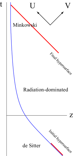
Figure 1: Brane trajectory in static coordinates.

II.2 Minkowski and de Sitter braneworlds

Let us consider tensor perturbations in AdS spacetime bounded by a brane. We can decompose the graviton field into a zero mode and Kaluza-Klein (KK) modes without ambiguity when the brane is maximally symmetric. This is the reason why the initial and final stages of the background model are given by the de Sitter and Minkowski phases, respectively.

We write the perturbed metric as

$$ds^{2}=\frac{\ell^{2}}{z^{2}}\left[-dt^{2}+(\delta_{ij}+h_{ij})dx^{i}dx^{j}+dz^{2}\right],$$ (4)

where $h_{ij}$ is the transverse-traceless metric perturbation. As usual we decompose it into the spatial Fourier modes as

$$h_{ij}=\frac{\sqrt{2}}{(2\pi M_{5})^{3/2}}\int d^{3}k~{}\phi_{{\bf k}}e^{i{\bf k}\cdot{\bf x}}e_{ij}.$$ (5)

Here $M_{5}$ is the fundamental mass scale which is related to the four-dimensional Planck mass $M_{{\rm Pl}}$ by $\ell(M_{5})^{3}=M_{{\rm Pl}}^{2}$. The prefactor $\sqrt{2}/(M_{5})^{3/2}$ is chosen so that the kinetic term for $\phi_{{\bf k}}$ in the effective action is canonically normalized. From now on we suppress the subscript ${\bf k}$.

For the analysis of perturbations from the Minkowski brane, the above Poincaré coordinate system will be best suited, and the perturbation equation is

$$\left(\frac{\partial^{2}}{\partial t^{2}}+k^{2}-\frac{\partial^{2}}{\partial z^{2}}+\frac{3}{z}\frac{\partial}{\partial z}\right)\phi=0,$$ (6)

subject to the boundary condition

$$\partial_{z}\phi\big{|}_{z=\ell}=0.$$ (7)

Now it is easy to find mode solutions of Eq. (6). Going to quantum theory, the graviton field can be expanded in terms of the zero mode and KK modes as

$$\phi=\hat{A}_{0}\varphi_{0}+\hat{A}_{0}^{\dagger}\varphi_{0}^{*}+\int_{0}^{\infty}\!\!dm\left(\hat{A}_{m}\varphi_{m}+\hat{A}_{m}^{\dagger}\varphi_{m}^{*}\right),$$ (8)

where $\hat{A}_{n}$ and $\hat{A}_{n}^{\dagger}$ ($n=0,m$) are the annihilation and creation operators, respectively, of their corresponding modes. The normalized zero mode function is given by

$$\varphi_{0}(t)=\frac{1}{\sqrt{2k\ell}}e^{-ikt},$$ (9)

while the normalized KK mode function is

$$\varphi_{m}(t,z)=\frac{1}{\sqrt{2\omega\ell^{3}}}e^{-i\omega t}u_{m}(z),$$ (10)

with

$$u_{m}(z):=z^{2}\sqrt{\frac{m}{2}}\frac{Y_{1}(m\ell)J_{2}(mz)-J_{1}(m\ell)Y_{2}(mz)}{\sqrt{[Y_{1}(m\ell)]^{2}+[J_{1}(m\ell)]^{2}}},$$ (11)

and

$$\omega=\sqrt{k^{2}+m^{2}}.$$ (12)

The normalization here is determined by the Wronskian conditions

$$(\varphi_{0}\cdot\varphi_{0})=-(\varphi_{0}^{*}\cdot\varphi_{0}^{*})=1,$$ (13)

$$(\varphi_{m}\cdot\varphi_{m^{\prime}})=-(\varphi_{m}^{*}\cdot\varphi_{m^{\prime}}^{*})=\delta(m-m^{\prime}),$$

$$(\varphi_{0}\cdot\varphi_{m})=(\varphi_{0}^{*}\cdot\varphi_{m}^{*})=0,$$

$$(\varphi_{n}\cdot\varphi_{n^{\prime}}^{*})=0,\qquad\mbox{for}\quad n,n^{\prime}=0,m,$$

where the Wronskian is defined by Gorbunov:2001ge

$$(X\cdot Y):=-2i\int^{\infty}_{\ell}dz\left(\frac{\ell}{z}\right)^{3}\left(X\partial_{t}Y^{*}-Y^{*}\partial_{t}X\right).$$ (14)

In the de Sitter braneworld we introduce another set of coordinates $(\eta,\xi)$, which is related to $(t,z)$ as

$$t=\eta\cosh\xi+t_{0},\quad z=-\eta\sinh\xi,$$ (15)

where $t_{0}$ is an arbitrary constant. In $(\eta,\xi)$ frame the de Sitter brane is located at a fixed coordinate position $\xi=\xi_{b}=$ constant, and the Hubble parameter on the brane is given by $H_{i}=\ell^{-1}\sinh\xi_{b}$. The perturbation equation again has a separable form

$$\left(\frac{\partial^{2}}{\partial\eta^{2}}-\frac{2}{\eta}\frac{\partial}{\partial\eta}+k^{2}-\frac{\sinh^{3}\xi}{\eta^{2}}\frac{\partial}{\partial\xi}\frac{1}{\sinh^{3}\xi}\frac{\partial}{\partial\xi}\right)\phi=0,$$ (16)

subject to the boundary condition

$$\partial_{\xi}\phi\big{|}_{\xi=\xi_{b}}=0.$$ (17)

Treating $\phi$ as an operator, the graviton field can be expanded as

$$\phi=\hat{a}_{0}\phi_{0}+\hat{a}_{0}^{\dagger}\phi_{0}^{*}+\int_{0}^{\infty}\!\!d\nu\left(\hat{a}_{\nu}\phi_{\nu}+\hat{a}_{\nu}^{\dagger}\phi_{\nu}^{*}\right),$$ (18)

where $\hat{a}_{n}$ and $\hat{a}_{n}^{\dagger}$ ($n=0,\nu$) are the annihilation and creation operators of each mode. The explicit form of the normalized zero mode is

$$\phi_{0}(\eta)=C(\ell H_{i})\cdot\frac{H_{i}}{\sqrt{2k\ell}}\left(\eta-\frac{i}{k}\right)e^{-ik\eta},$$ (19)

with

$$C(x):=\left[\sqrt{1+x^{2}}+x^{2}\ln\left(\frac{x}{1+\sqrt{1+x^{2}}}\right)\right]^{-1/2},$$ (20)

and the KK mode functions are found in the form of $\phi_{\nu}(\eta,\xi)=\psi_{\nu}(\eta)\chi_{\nu}(\xi)$, where

$$\psi_{\nu}(\eta) = \frac{\sqrt{\pi}}{2}\ell^{-3/2}e^{-\pi\nu/2}(-\eta)^{3/2}H^{(1)}_{i\nu}(-k\eta),$$ (21)

$$\chi_{\nu}(\xi) = C_{1}(\sinh\xi)^{2}\left[P^{-2}_{-1/2+i\nu}(\cosh\xi)\right.$$ (22)

$$\quad\left.-C_{2}Q^{-2}_{-1/2+i\nu}(\cosh\xi)\right],$$

with

$$C_{1} = \left[\left|\frac{\Gamma(i\nu)}{\Gamma(5/2+i\nu)}\right|^{2}\right.$$ (23)

$$\left.+\left|\frac{\Gamma(-i\nu)}{\Gamma(5/2-i\nu)}-\pi C_{2}\frac{\Gamma(i\nu-3/2)}{\Gamma(1+i\nu)}\right|^{2}\right]^{-1/2},$$

$$C_{2} = \frac{P^{-1}_{-1/2+i\nu}(\cosh\xi_{b})}{Q^{-1}_{-1/2+i\nu}(\cosh\xi_{b})}.$$ (24)

Note that the index $\nu(\geq 0)$ is related to the Kaluza-Klein mass as

$$m^{2}=\left(\nu^{2}+\frac{9}{4}\right)H_{i}^{2}.$$ (25)

The normalization of the modes is determined by the Wronskian conditions

$$(\phi_{0}\cdot\phi_{0})=-(\phi_{0}^{*}\cdot\phi_{0}^{*})=1,$$ (26)

$$(\phi_{\nu}\cdot\phi_{\nu^{\prime}})=-(\phi_{\nu}^{*}\cdot\phi_{\nu^{\prime}}^{*})=\delta(\nu-\nu^{\prime}),$$

$$(\phi_{0}\cdot\phi_{\nu})=(\phi_{0}^{*}\cdot\phi_{\nu}^{*})=0,$$

$$(\phi_{n}\cdot\phi_{n^{\prime}}^{*})=0,\qquad\mbox{for}\quad n,n^{\prime}=0,\nu.$$

Here the Wronskian is written in $(\eta,\xi)$ frame as Gorbunov:2001ge ,

$$(X\cdot Y):=-2i\int^{\infty}_{\xi_{b}}d\xi\frac{\ell^{3}}{\eta^{2}\sinh^{3}\xi}\left(X\partial_{\eta}Y^{*}-Y^{*}\partial_{\eta}X\right).$$

III Wronskian formulation

Due to the presence of an infinite tower of Kaluza-Klein modes, cosmological perturbations in the braneworld have infinite degrees of freedom. Instead of solving an initial value problem for such a system, it would be better to use the Wronskian formulation in order to take necessary degrees of freedom out of infinite information. In the present case, we would like to know the final amplitude of the zero mode, and therefore in fact what we need to do is solving the (backward) evolution of a single degree of freedom Gorbunov:2001ge ; Kobayashi:2003cn ; Kobayashi:2005jx . Following the same line as our previous work Kobayashi:2005jx , we now explain how we compute the amplitude of gravitational waves in the final Minkowski phase using the Wronskian.

Using double null coordinates

$$u=t-z,$$ (28)

$$v=t+z,$$ (29)

which will be convenient for numerical calculations, the metric (1) can be rewritten in the form of

$$ds^{2}=\frac{4\ell^{2}}{(v-u)^{2}}\left(-dudv+\delta_{ij}dx^{i}dx^{j}\right).$$ (30)

The trajectory of the brane can be specified arbitrarily by

$$v=q(u).$$ (31)

By a further coordinate transformation

$$U=u,$$ (32)

$$q(V)=v,$$ (33)

we obtain

$$ds^{2}=\frac{4\ell^{2}}{[q(V)-U]^{2}}\left[-q^{\prime}(V)dUdV+\delta_{ij}dx^{i}dx^{j}\right],$$ (34)

where a prime denotes differentiation with respect to the argument. Now in the new coordinates the position of the brane is simply given by

$$U=V.$$ (35)

We will use this coordinate system for actual numerical calculations.

The induced metric on the brane is

$$ds_{b}^{2}=\frac{4\ell^{2}}{[q(V)-V]^{2}}\left[-q^{\prime}(V)dV^{2}+\delta_{ij}dx^{i}dx^{j}\right],$$ (36)

from which we can read off the scale factor $a$ and the proper time $\tau$, respectively, as

$$a=\frac{2\ell}{q(V)-V},$$ (37)

$$d\tau=a\sqrt{q^{\prime}(V)}~{}dV,$$ (38)

and hence the Hubble parameter on the brane is written as

$$\ell H=\frac{1}{2\sqrt{q^{\prime}(V)}}[1-q^{\prime}(V)],$$ (39)

or equivalently

$$q^{\prime}(V)=\left(\sqrt{1+\ell^{2}H^{2}}-\ell H\right)^{2}.$$ (40)

Given the Hubble parameter as a function of $\tau$, one can integrate Eqs. (38) and (40) with the aid of $da/d\tau=aH$ to obtain $q$ as a function of $V$. If the Hubble parameter on the brane is constant in time, we have $q^{\prime}=$ constant. Especially, $q^{\prime}=1$ in the Minkowski phase.

The Klein-Gordon-type equation for a gravitational wave perturbation $\phi$ in the $(U,V)$ coordinates reduces to

$$\!\left[4\partial_{U}\partial_{V}+\frac{6}{q(V)-U}(\partial_{V}-q^{\prime}(V)\,\partial_{U})+q^{\prime}(V)\,k^{2}\right]\phi=0,\!\!\!$$ (41)

(42)

supplemented by the boundary condition

$$[\partial_{U}-\partial_{V}]\phi\bigr{|}_{U=V}=0.$$ (43)

The expression for the Wronskian evaluated on a constant $V$ hypersurface is given by

$$(X\cdot Y)={2i}\!\int^{V}_{-\infty}\!\!\!dU\!\left[\frac{2\ell}{q(V)-U}\right]^{3}\!(X\partial_{U}Y^{*}\!-Y^{*}\partial_{U}X),$$ (44)

which is independent of the choice of the hypersurface.

As explained in Section II, our cosmological model is composed of the de Sitter inflationary phase followed by the radiation-dominated epoch, which is connected smoothly to the final Minkowski phase. In the initial de Sitter phase, the graviton field can be expanded as Eq. (18), while in the final Minkowski phase it can be expanded as Eq. (8). We assume that initially the gravitons are in the de Sitter invariant vacuum state annihilated by $\hat{a}_{0}$ and $\hat{a}_{\nu}$,

$$\hat{a}_{0}|0\rangle=\hat{a}_{\nu}|0\rangle=0.$$ (46)

The expectation value of the squared amplitude of the zero mode in the final stage is

$$\langle 0|\left(\varphi_{0}\hat{A}_{0}+\varphi^{*}_{0}\hat{A}_{0}^{\dagger}\right)^{2}|0\rangle = |\varphi_{0}|^{2}\langle 0|\left(1+2\hat{A}_{0}^{\dagger}\hat{A}_{0}\right)|0\rangle$$

$$+~{}\mbox{oscillating part}$$

$$\simeq \frac{1}{k\ell}N_{f},$$

where $N_{f}:=\langle 0|\hat{A}_{0}^{\dagger}\hat{A}_{0}|0\rangle$ is the number of created zero mode gravitons. Here we used the commutation relation $\left[\hat{A}_{0},\hat{A}_{0}^{\dagger}\right]=1$ and assumed that $N_{f}\gg 1$. The final power spectrum is then given by

$${\cal P}(k) := \frac{4\pi k^{3}}{(2\pi)^{3}}\frac{2}{(M_{5})^{3}}\cdot\frac{1}{k\ell}N_{f}$$ (47)

$$= \frac{k^{2}}{\pi^{2}M_{{\rm Pl}}^{2}}N_{f}.$$

The operator $\hat{A}_{0}$ can be projected out by making use of the Wronskian relations. Noting that the Wronskian is constant in time, we have

$$\hat{A}_{0} = (\phi\cdot\varphi_{0})_{f}=(\phi\cdot\Phi)$$ (48)

$$= (\phi_{0}\cdot\Phi)_{i}\hat{a}_{0}+\int d\nu(\phi_{\nu}\cdot\Phi)_{i}\hat{a}_{\nu}+~{}\mbox{h.c.},$$

where $\Phi$ is a solution of the Klein-Gordon equation (42) whose final configuration is the zero mode function $\varphi_{0}$ in the Minkowski phase, and subscript $f$ and $i$ denote the quantities evaluated on the final and initial hypersurfaces, respectively. Thus we clearly see that final zero mode gravitons are created from the vacuum fluctuations both in the initial zero mode and in the KK modes:

$$N_{f}=|(\phi_{0}^{*}\cdot\Phi)_{i}|^{2}+\int d\nu|(\phi_{\nu}^{*}\cdot\Phi)_{i}|^{2}.$$ (49)

Correspondingly, the power spectrum (47) can be written as a sum of the two contributions:

$${\cal P}={\cal P}_{0}+{\cal P}_{{\rm KK}},$$ (50)

where

$${\cal P}_{0} := \frac{k^{2}}{\pi^{2}M_{{\rm Pl}}^{2}}|(\phi_{0}^{*}\cdot\Phi)_{i}|^{2},$$ (51)

$${\cal P}_{{\rm KK}} := \frac{k^{2}}{\pi^{2}M_{{\rm Pl}}^{2}}\int d\nu|(\phi_{\nu}^{*}\cdot\Phi)_{i}|^{2}.$$ (52)

IV Spectrum of gravitational waves

De Sitter inflation on the brane predicts the flat primordial spectrum Langlois:2000ns

$$\delta_{T}^{2}:=\frac{2C^{2}(\ell H_{i})}{M_{{\rm Pl}}^{2}}\left(\frac{H_{i}}{2\pi}\right)^{2}.$$ (53)

During inflation the gravitational wave perturbations are stretched to super-horizon scales, and then they stays constant until horizon reentry, with their amplitude given by Eq. (53). ($\phi=$ constant is a growing solution of Eq. (42) in the limit $k^{2}\to 0$.) The primordial spectrum of gravitational waves from non-de Sitter inflation was studied extensively in Kobayashi:2005jx , and so in this paper we concentrate on the simple case where inflation is given by the exact de Sitter model.

For long wavelength modes with $k\ll k_{*}$, where

$$k_{*}:=a_{*}H_{*}=a_{*}/\ell$$ (54)

labels the mode that reenters the horizon when $\ell H=1$, the amplitude will decay as $h_{\mu\nu}\propto a^{-1}$ after horizon reentry, because gravity on the brane is basically described by four-dimensional general relativity in the low energy regime ($\ell H\ll 1$). In fact, it is explicitly shown that leading order corrections to the cosmological evolution of gravitational waves are suppressed by $\ell^{2}$ and $\ell^{2}\ln\ell$ at low energies Tanaka:2004ig ; Kobayashi:2004wy . In particular, modes with $k<k_{0}$, where

$$k_{0}:=a_{0}H_{0}=H_{0},$$ (55)

and $H_{0}$ is the Hubble parameter evaluated at the end of the radiation-dominated phase (i.e., just before the Minkowski phase), reenter the “horizon” in the final Minkowski phase, and then they begin to oscillate (but their amplitude will not decay). As a result, the mean-square vacuum fluctuations of such modes become half of the initial value, leading to

$${\cal P}=\frac{\delta_{T}^{2}}{2},\quad\mbox{for}~{}k<k_{0}.$$ (56)

In Ref. Gorbunov:2001ge , the same spectrum was obtained for scales larger than the AdS and horizon scales by using the “junction model”, in which an instantaneous transition from a de Sitter to a Minkowski brane was assumed. For the reason mentioned above, modes with $k_{0}<k\ll k_{*}$ have the standard spectrum,

$${\cal P}=\frac{\delta_{T}^{2}}{2}\left(\frac{k}{k_{0}}\right)^{-2}.$$ (57)

Something nontrivial may happen to gravitational waves with $k\gtrsim k_{*}$. If the effects of mode mixing are neglected, only the modification of the background expansion rate alters the spectrum for these short wavelength modes to

$$\tilde{\cal P}\simeq\frac{\delta_{T}^{2}}{2}\left(\frac{k}{k_{*}}\right)^{-2/3}\left(\frac{k_{*}}{k_{0}}\right)^{-2}.$$ (58)

However, this evaluation will not be correct because mode mixing is expected to be efficient at high energies.

Our procedure to obtain a correct power spectrum is as follows. We solve the perturbation equation (42) with its boundary condition set to be $\Phi(U,V_{f})=\varphi_{0}$ on the final hypersurface. The numerical backward evolution scheme we use here is the same as that used in our previous work Kobayashi:2005jx , and the detailed description of the scheme is found there. After obtaining the configuration on the initial hypersurface, we evaluate the Wronskian to get the power spectrum.

We performed numerical calculations for three different values of the inflationary Hubble parameter, $\ell H_{i}=10$, $42$, and $100$. The radiation-dominated phase is terminated when the Hubble parameter decreases down to $H\simeq 0.03/\ell=:H_{0}$, and then it is connected smoothly to the Minkowski phase, so that we can see the amplitude of the well-defined zero mode. The numbers of grids are 90000 in the $U$-direction and 12000 in the $V$-direction, and the grid separation is chosen to be $\sim 0.005\times\ell$. Integration over the KK index $\nu$ is performed up to $\nu=25$ with an equal grid spacing of $0.05$.

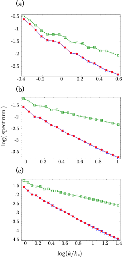
Figure 2: Power spectra of gravitational waves from inflation with $\ell H_{i}=10$ (a), $42$ (b), and $100$ (c), normalized by $\delta_{T}^{2}/2$. The total power spectrum is shown by red circles, while blue crosses represent the contribution only from the initial zero mode. Green squires indicate results from basically four-dimensional calculations, only including the effect of the modification of the background expansion rate.

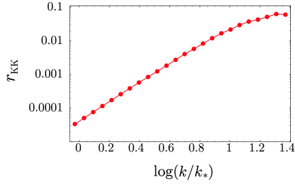
Figure 3: Contribution of initial Kaluza-Klein fluctuations, $r_{{\rm KK}}$, for the model with $\ell H_{i}=100$.

The power spectra of gravitational waves are shown in Fig. 2. Assuming that the power spectrum is of the form

$${\cal P}=A\left(\frac{k}{k_{0}}\right)^{n},$$ (59)

we find that irrespective of the inflationary energy scale, the parameters are approximately given by

$$A \simeq \frac{\delta_{T}^{2}}{2},$$ (60)

$$n \simeq -2.$$ (61)

Namely, we have the same spectrum as the standard one [Eq. (57)] even for short wavelength modes with $k\gtrsim k_{*}$. As is shown in Fig. 3, the contribution of the vacuum fluctuations in the initial KK modes to the final spectrum,

$$r_{{\rm KK}}(k):=\frac{{\cal P}_{{\rm KK}}}{{\cal P}_{0}+{\cal P}_{{\rm KK}}},$$ (62)

never exceeds 10% so far as the present calculations are concerned, and hence it gives a subdominant effect. On the other hand, the excitation of KK modes suppresses the amplitude of the gravitational waves relative to Eq. (58), and our result implies that the effect of the modification of the background Friedmann equation compensate this suppression, leading to approximately the same spectral tilt as that in conventional four-dimensional cosmology. This is consistent with the numerical study by Hiramatsu et al. Hiramatsu:2004aa , in which they assume the initial configuration in the bulk to be a de Sitter zero mode and obtain ${\cal P}_{0}\propto k^{-2}$.

Figure 4: $r_{{\rm KK}}$ for $\ell H_{i}=100$ and $k=13.3\times k_{*}$, versus the number of grids in the $U$-direction.

Unfortunately, due to the limited number of grids in the $U$-direction, it is difficult to evaluate accurate values of $r_{{\rm KK}}$; the convergence is not so good (Fig. 4). However, since $r_{{\rm KK}}$ decreases with an increasing number of grids, it is strongly expected that the effect of the initial KK fluctuations is negligibly small. To obtain a more accurate evaluation of the contribution of the initial KK modes, we need an improved numerical formulation, though it seems quite unlikely that $r_{{\rm KK}}$ turns to increase at a much larger number of grids. (We confirmed that the convergence of the zero mode part ${\cal P}_{0}$ is sufficiently good.)

V Generation of dark radiation

So far we have concentrated on final zero mode gravitons created from initial vacuum fluctuations. In this section we shall discuss the generation of KK gravitons. In particular, we are interested in the KK mode gravitons created from initial fluctuations in the zero mode, because from the five-dimensional point of view they are interpreted as gravitons that escape from the brane. At sufficiently late times, all the emitted gravitons fall deep into the bulk, and then the bulk spacetime is described as an AdS-Schwarzschild black hole, the mass of which divided by $a^{4}$ is viewed as the “dark radiation” from a brane observer Hebecker:2001nv ; Langlois:2002ke ; Langlois:2003zb ; Leeper:2003dd .

Before going to the estimation of the energy density of final KK mode gravitons, first let us take a look at the energy density of zero mode gravitons $\rho_{{\rm GW}}$. Since at low energies gravitational waves evolve in a standard manner, their energy density behaves as $\rho_{{\rm GW}}\propto a^{-4}$. Therefore the ratio $\rho_{{\rm GW}}/\rho_{r}$ is an invariant quantity in the low energy regime, irrespective of the cosmic expansion. Evaluating it at the end of the radiation stage, we have

$$\frac{\rho_{{\rm GW}}}{\rho_{r}}=\frac{\rho_{{\rm GW},0}}{\rho_{r,0}}\simeq\ln\left(\frac{k_{i}}{k_{0}}\right)\cdot\frac{\delta_{T}^{2}}{6}\sim\delta_{T}^{2}.$$ (63)

Note that $\delta_{T}<10^{-5}$. In deriving the estimate (63), we used the formula

$$\rho_{{\rm GW},0}=M_{{\rm Pl}}^{2}\int_{k_{0}}^{k_{i}}\!\!d\ln k~{}k^{2}{\cal P}(k),$$ (64)

and substituted the numerical result obtained in the previous section, ${\cal P}\simeq(\delta_{T}^{2}/2)(k/k_{0})^{-2}$, where $k_{0}$ can be eliminated in favor of $\rho_{r,0}$ by using the Friedmann equation at low energies $k_{0}^{2}=H_{0}^{2}\simeq\rho_{r,0}/(3M_{{\rm Pl}}^{2}).$ The upper limit of the integral may be given by the inverse horizon scale at the end of inflation,

$$k_{i}:=a_{i}H_{i},$$ (65)

because the particle production is exponentially suppressed on sub-horizon scales.

Let $\tilde{\rho}_{{\rm GW}}$ be the energy density of gravitational waves obtained by neglecting the mode mixing effect. More precisely, $\tilde{\rho}_{{\rm GW}}$ is the energy density of gravitational waves $h_{\mu\nu}$ where $h_{\mu\nu}$ is a solution of the conventional perturbation equation $(\partial^{2}_{\tau}+3H\partial_{\tau}+k^{2}/a^{2})h_{\mu\nu}=0$ with the cosmic expansion given by a solution of the modified Friedmann equation. This would be much greater than $\rho_{{\rm GW}}$. Then, $\Delta\rho:=\tilde{\rho}_{{\rm GW}}-\rho_{{\rm GW}}\simeq\tilde{\rho}_{{\rm GW}}$ is the energy density that leaks from the brane, and by definition $\Delta\rho$ is proportional to $a^{-4}$ as long as it is evaluated in the low energy regime. Thus, $\Delta\rho/\rho_{r}$ is an invariant quantity. Now $\Delta\rho_{,0}$ can be calculated from the spectrum of the form (58), and we have an estimate

$$\frac{\Delta\rho}{\rho_{r}}=\frac{\Delta\rho_{,0}}{\rho_{r,0}}\simeq\frac{\delta_{T}^{2}}{8}\times\ell H_{i},$$ (66)

where we used $a^{4}\rho_{r}=a_{*}^{4}\sigma=\rho_{r,0}$ and the Friedmann equation at high energies, $H^{2}\simeq\rho^{2}/6M_{{\rm Pl}}^{2}\sigma$. The estimate (66) implies that a large amount of energy (compared to $\rho_{{\rm GW}}$) is lost from the brane. Is the escaped energy $\Delta\rho$ directly transferred to the final bulk gravitons? To discuss this point, we compare it with the energy density of the generated dark radiation.

Since KK modes are excited dominantly at high energies but not at low energies, the dark radiation, as is deduced from its name, behaves like a radiation component, $\rho_{{\rm DR}}\propto a^{-4}$, at late times. Hence, we shall see the ratio $\rho_{{\rm DR}}/\rho_{r}$ but it may be evaluated at the end of the radiation stage.

The total number of the created bulk gravitons is given again by the Wronskian as

$$\int dm\langle 0|\hat{A}_{m}^{\dagger}\hat{A}_{m}|0\rangle=$$

$$\qquad\int dm\left[|(\phi_{0}^{*}\cdot\Phi_{m})_{i}|^{2}+\int d\nu|(\phi_{\nu}^{*}\cdot\Phi_{m})_{i}|^{2}\right],$$

where $\Phi_{m}$ is a solution of the Klein-Gordon equation (42) whose final configuration is a KK mode function $\varphi_{m}$ in the Minkowski phase. Concentrating on the first part, $|(\phi_{0}^{*}\cdot\Phi_{m})|^{2}dm$ is identified as the number of KK gravitons coming from the initial zero mode fluctuations, with their mass between $m$ and $m+dm$. Thus the energy density is expressed as

$$\rho_{{\rm DR},0} := \int\frac{d^{3}k}{(2\pi)^{3}}\int dm~{}\omega|(\phi_{0}^{*}\cdot\Phi_{m})_{i}|^{2}$$ (67)

$$= \int d\ln k\int d\ln m~{}\frac{mk^{3}\omega}{2\pi^{2}}|(\phi_{0}^{*}\cdot\Phi_{m})_{i}|^{2}.$$

As a side remark, in the junction model of Ref. Gorbunov:2001ge , the second part, i.e., the number of KK gravitons created from the initial fluctuations in KK modes, is suppressed compared to the first one.

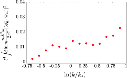
Figure 5: Energy of bulk gravitons multiplied by the phase space factor.

We numerically calculated the Wronskian $|(\phi_{0}^{*}\cdot\Phi_{m})|^{2}$ in a similar manner to the previous section. The Hubble parameter during inflation is chosen to be $\ell H_{i}=42$. In this case, the number of grids are 150000 in the $U$-direction and 20000 in the $V$-direction, and the grid separation is about $0.0036\times\ell$.

The integrand

$$\int d\ln m~{}\frac{mk^{3}\omega}{2\pi^{2}}|(\phi_{0}^{*}\cdot\Phi_{m})_{i}|^{2}$$

is plotted in Fig. 5. For each $k$, integration over $m$ is performed up to $m\sim 2/\ell$ with a grid spacing of $\Delta\ln m\simeq 0.17$. Performing the integration over $k$, we obtain

$$\rho_{{\rm DR},0}\approx 0.04\times\ell^{-4},$$ (68)

where one should note that contributions from modes with $k<k_{*}$ are suppressed. The radiation energy density can be written as

$$\rho_{r,0}=a_{i}^{4}\rho_{r,i}\simeq a_{i}^{4}(6M_{{\rm Pl}}^{2}\sigma)^{1/2}H_{i}\simeq\frac{9}{2\pi^{2}}\frac{1}{\delta_{T}^{2}}(a_{i}H_{i})^{4},$$ (69)

which can be obtained by using the modified Friedmann equation and noting that $\delta_{T}^{2}\simeq 3\ell H_{i}^{3}/4\pi^{2}M_{{\rm Pl}}^{2}$ for $\ell H_{i}\gg 1$. From Eqs. (68) and (69) we have an estimate

$$\frac{\rho_{{\rm DR}}}{\rho_{r}}<{\cal O}(1)\times\delta_{T}^{2}.$$ (70)

This result indicates that the energy density of the generated dark radiation is not larger than that of zero mode gravitons [Eq. (63)]. Of course, this is a completely harmless amount of an extra radiation component Ichiki:2002eh . The scattering of particles on the brane in the early universe, discussed in Hebecker:2001nv ; Langlois:2002ke ; Langlois:2003zb ; Leeper:2003dd , can be a more efficient way to produce bulk gravitons.

Although a large amount of energy is lost from the brane via excitation of KK modes in the high energy regime, the final energy density of the dark radiation is much smaller than that, without an enhancement factor like $\ell H_{i}$ in Eq. (66). This discrepancy is explained as follows Hebecker:2001nv ; Langlois:2003zb . In the high energy regime, the motion of the brane is so relativistic (in the frame defined by the static bulk coordinates) that emitted gravitons run almost parallel to the brane trajectory. These gravitons stay in the vicinity of the brane and bounce off it many times during the high energy stage, until eventually they are reflected by the non-relativistic brane to fall off into the bulk. During this process, the gravitons lose a large portion of their momentum transverse to the brane because they repeatedly hit the retreating brane. This qualitatively accounts for the smallness of the final energy density of the dark radiation. To justify the above interpretation quantitatively, a more rigorous analysis will be needed in the direction of Refs. Langlois:2003zb ; Minamitsuji:2005xs , which includes calculating the pressure to the brane due to the effective energy-momentum tensor of the bulk gravitational waves.

Here we should comment on the result of the junction model obtained by Gorbunov et al. Gorbunov:2001ge . In terms of the power spectrum, their result is summarized as

$${\cal P}\approx\left\{{\displaystyle\frac{\delta_{T}^{2}}{2},\qquad(k\ll k_{*}),}\atop{\displaystyle\frac{\delta_{T}^{2}}{2}\frac{4}{(k/k_{*})^{2}},\quad(k_{*}\ll k\ll k_{i}),}\right.$$ (71)

where $k_{*}=a_{*}/\ell$, $k_{i}=a_{i}H_{i}$, and $a_{*}=a_{i}(=1)$ because a de Sitter inflationary stage is directly joined to a Minkowski phase in the junction model (see also Appendix A of Ref. Kobayashi:2003cn ). From this we can estimate the energy density that leaks from the brane as

$$\Delta\rho\approx M_{{\rm Pl}}^{2}H_{i}^{2}\delta_{T}^{2}\approx\rho_{e.i.}\delta_{T}^{2}\times\ell H_{i},$$ (72)

where $\rho_{e.i.}$ is the energy density at the “end of inflation”. On the other hand, according to Appendix D of Ref. Gorbunov:2001ge , the energy density of created KK gravitons is given by

$$\rho_{{\rm DR}}\approx H_{i}^{4}\approx\rho_{e.i.}\delta_{T}^{2}.$$ (73)

Thus, we find that $\Delta\rho\sim\rho_{{\rm DR}}\times\ell H_{i}$, which is consistent with our present result. [Note that in the junction model the energy density of final zero mode gravitons is estimated as $\rho_{{\rm GW}}\sim(M_{{\rm Pl}}^{2}/\ell^{2})\delta_{T}^{2}$ and hence $\rho_{{\rm GW}}\ll\rho_{e.i.}\delta_{T}^{2}\sim\rho_{{\rm DR}}$.]

VI Summary

We have examined the power spectrum of the gravitational wave background in the cosmological scenario of the Randall-Sundrum braneworld. There are three possible ingredients which may lead the power spectrum to a non-standard one: the unconventional background expansion rate due to the $\rho^{2}$ term in the Friedmann equation, the excitation of KK modes during the radiation-dominated stage at high energies, and the effect of initial vacuum fluctuations in KK modes. Previous estimates are based on a rather simple toy model Gorbunov:2001ge or numerical studies about the classical evolution of perturbations, neglecting the initial KK fluctuations Hiramatsu:2003iz ; Hiramatsu:2004aa . In the present analysis, initial conditions are set in a quantum-mechanical manner and hence the effect of the initial KK fluctuations is included. Along the same line in Ref. Kobayashi:2005jx , we make use of the Wronskian formulation to obtain the final amplitude of the zero mode gravitational waves numerically. We have found that the effect of initial KK vacuum fluctuations are subdominant: $r_{{\rm KK}}<0.1$. Our result confirms that the damping of the amplitude due to the KK mode excitation and the enhancement due to the modification of the background expansion rate mainly work, but almost cancel each other. Consequently, the power spectrum is basically the same as the standard one obtained in conventional four-dimensional cosmology. We believe that the cancellation between the two effects is a phenomenon peculiar to the radiation-dominated phase. To make the particularity of the radiation stage clear, it would be interesting to investigate consequences of a different equation of state parameter $w(=p/\rho)$ after the inflationary stage. This is the next issue we plan to report in a future publication.

Because of the limitation of our numerical computation, we have not been able to give a detailed evaluation of how much the initial KK fluctuations contribute to the final power spectrum. Although it is strongly indicated that the initial KK effect never becomes larger than the present evaluation, to show that it is indeed true, we need to improve the numerical formulation. We will also report on this issue in a forthcoming paper.

We have also estimated the energy density of the generated dark radiation numerically, and shown that only a tiny amount is generated. It is smaller than the energy density of zero mode gravitational waves.

- (1) For a review, see, e.g., M. Maggiore, Phys. Rept. 331, 283 (2000) [arXiv:gr-qc/9909001].
- (2) For a review, see, e.g., R. Maartens, Living Rev. Rel. 7, 7 (2004) [arXiv:gr-qc/0312059].
- (3) L. Randall and R. Sundrum, Phys. Rev. Lett. 83, 3370 (1999) [arXiv:hep-ph/9905221].
- (4) L. Randall and R. Sundrum, Phys. Rev. Lett. 83, 4690 (1999) [arXiv:hep-th/9906064].
- (5) J. Garriga and T. Tanaka, Phys. Rev. Lett. 84, 2778 (2000) [arXiv:hep-th/9911055], S. B. Giddings, E. Katz and L. Randall, JHEP 0003, 023 (2000) [arXiv:hep-th/0002091].
- (6) T. Shiromizu, K. i. Maeda and M. Sasaki, Phys. Rev. D 62, 024012 (2000) [arXiv:gr-qc/9910076].
- (7) R. Maartens, D. Wands, B. A. Bassett and I. Heard, Phys. Rev. D 62, 041301 (2000) [arXiv:hep-ph/9912464], S. Mukohyama, Phys. Rev. D 62, 084015 (2000) [arXiv:hep-th/0004067], H. Kodama, A. Ishibashi and O. Seto, Phys. Rev. D 62, 064022 (2000) [arXiv:hep-th/0004160], D. Langlois, Phys. Rev. D 62, 126012 (2000) [arXiv:hep-th/0005025], D. Langlois, Phys. Rev. Lett. 86, 2212 (2001) [arXiv:hep-th/0010063], H. A. Bridgman, K. A. Malik and D. Wands, Phys. Rev. D 63, 084012 (2001) [arXiv:hep-th/0010133], D. Langlois, R. Maartens, M. Sasaki and D. Wands, Phys. Rev. D 63, 084009 (2001) [arXiv:hep-th/0012044], H. A. Bridgman, K. A. Malik and D. Wands, Phys. Rev. D 65, 043502 (2002) [arXiv:astro-ph/0107245], K. Koyama and J. Soda, Phys. Rev. D 62, 123502 (2000) [arXiv:hep-th/0005239], K. Koyama and J. Soda, Phys. Rev. D 65, 023514 (2002) [arXiv:hep-th/0108003], B. Gumjudpai, R. Maartens and C. Gordon, Class. Quant. Grav. 20, 3295 (2003) [arXiv:gr-qc/0304067], K. Koyama, Phys. Rev. D 66, 084003 (2002) [arXiv:gr-qc/0204047], K. Koyama, Phys. Rev. Lett. 91, 221301 (2003) [arXiv:astro-ph/0303108], C. S. Rhodes, C. van de Bruck, P. Brax and A. C. Davis, Phys. Rev. D 68, 083511 (2003) [arXiv:astro-ph/0306343], T. Kobayashi and T. Tanaka, Phys. Rev. D 69, 064037 (2004) [arXiv:hep-th/0311197], K. Koyama, JCAP 0409, 010 (2004) [arXiv:astro-ph/0407263], K. Koyama, D. Langlois, R. Maartens and D. Wands, JCAP 0411, 002 (2004) [arXiv:hep-th/0408222], C. de Rham, Phys. Rev. D 71, 024015 (2005) [arXiv:hep-th/0411021], H. Yoshiguchi and K. Koyama, Phys. Rev. D 71, 043519 (2005) [arXiv:hep-th/0411056], K. Koyama, A. Mennim and D. Wands, Phys. Rev. D 72, 064001 (2005) [arXiv:hep-th/0504201], K. Koyama, S. Mizuno and D. Wands, JCAP 0508, 009 (2005) [arXiv:hep-th/0506102],
- (8) D. Langlois, R. Maartens and D. Wands, Phys. Lett. B 489, 259 (2000) [arXiv:hep-th/0006007].
- (9) D. S. Gorbunov, V. A. Rubakov and S. M. Sibiryakov, JHEP 0110, 015 (2001) [arXiv:hep-th/0108017].
- (10) T. Kobayashi, H. Kudoh and T. Tanaka, Phys. Rev. D 68, 044025 (2003) [arXiv:gr-qc/0305006].
- (11) T. Kobayashi and T. Tanaka, Phys. Rev. D 71, 124028 (2005) [arXiv:hep-th/0505065].
- (12) T. Tanaka, arXiv:gr-qc/0402068.
- (13) T. Kobayashi and T. Tanaka, JCAP 0410, 015 (2004) [arXiv:gr-qc/0408021].
- (14) R. Easther, D. Langlois, R. Maartens and D. Wands, JCAP 0310, 014 (2003) [arXiv:hep-th/0308078].
- (15) R. A. Battye, C. Van de Bruck and A. Mennim, Phys. Rev. D 69, 064040 (2004) [arXiv:hep-th/0308134].
- (16) R. A. Battye and A. Mennim, Phys. Rev. D 70, 124008 (2004) [arXiv:hep-th/0408101].
- (17) C. Cartier, R. Durrer and M. Ruser, arXiv:hep-th/0510155.
- (18) T. Hiramatsu, K. Koyama and A. Taruya, Phys. Lett. B 578, 269 (2004) [arXiv:hep-th/0308072].
- (19) T. Hiramatsu, K. Koyama and A. Taruya, Phys. Lett. B 609, 133 (2005) [arXiv:hep-th/0410247].
- (20) K. Ichiki and K. Nakamura, Phys. Rev. D 70, 064017 (2004) [arXiv:hep-th/0310282].
- (21) K. Ichiki and K. Nakamura, arXiv:astro-ph/0406606.
- (22) J. C. Long, H. W. Chan, A. B. Churnside, E. A. Gulbis, M. C. M. Varney and J. C. Price, arXiv:hep-ph/0210004.
- (23) P. Binetruy, C. Deffayet and D. Langlois, Nucl. Phys. B 565, 269 (2000) [arXiv:hep-th/9905012], P. Binetruy, C. Deffayet, U. Ellwanger and D. Langlois, Phys. Lett. B 477, 285 (2000) [arXiv:hep-th/9910219], S. Mukohyama, Phys. Lett. B 473, 241 (2000) [arXiv:hep-th/9911165], D. Ida, JHEP 0009, 014 (2000) [arXiv:gr-qc/9912002], P. Kraus, JHEP 9912, 011 (1999) [arXiv:hep-th/9910149].
- (24) A. Hebecker and J. March-Russell, Nucl. Phys. B 608, 375 (2001) [arXiv:hep-ph/0103214].
- (25) D. Langlois, L. Sorbo and M. Rodriguez-Martinez, Phys. Rev. Lett. 89, 171301 (2002) [arXiv:hep-th/0206146].
- (26) D. Langlois and L. Sorbo, Phys. Rev. D 68, 084006 (2003) [arXiv:hep-th/0306281].
- (27) E. Leeper, R. Maartens and C. F. Sopuerta, Class. Quant. Grav. 21, 1125 (2004) [arXiv:gr-qc/0309080].
- (28) K. Ichiki, M. Yahiro, T. Kajino, M. Orito and G. J. Mathews, Phys. Rev. D 66, 043521 (2002) [arXiv:astro-ph/0203272].
- (29) M. Minamitsuji, M. Sasaki and D. Langlois, Phys. Rev. D 71, 084019 (2005) [arXiv:gr-qc/0501086].