Abstract

We study Dirac-Born-Infeld type effective field theory of a complex tachyon and U(1)$\times$U(1) gauge fields describing a D3${\bar{\rm D}}$3 system. Classical solutions of straight global and local DF-strings with quantized vorticity are found and are classified into two types by the asymptotic behavior of the tachyon amplitude. For sufficiently large radial distances, one has linearly-growing tachyon amplitude and the other logarithmically-growing tachyon amplitude. A constant radial electric flux density denoting the fundamental-string background makes the obtained DF-strings thick. The other electric flux density parallel to the strings is localized, which represents localization of fundamental strings in the D1-F1 bound states. Since these DF-strings are formed in the coincidence limit of the D3${\bar{\rm D}}$3, these cosmic DF-strings are safe from inflation induced by the approach of the separated D3 and ${\bar{\rm D}}3$.

1 Introduction

When we have a system of a D3-brane and an anti-D3-brane, its dynamics is well described by the effective field theory of a complex tachyon field and U(1)$\times$U(1) gauge fields [1, 2, 3]. While the D3 and ${\bar{\rm D}}3$ approach each other from apart, the Universe undergoes an inflationary era due to the gravitational effect [4]. When the D-brane coincides with the ${\bar{\rm D}}3$-brane, the system reaches the top of the tachyon potential and the main inflation ends. Then, this unphysical symmetric vacuum state at the zero tachyon amplitude restarts to decay to the true U(1) degenerate vacua at an infinite tachyon amplitude.

When the D3-brane and ${\bar{\rm D}}3$-brane are annihilated in their coincidence limit, perturbative open string degrees living on the branes disappear, but nonperturbative open string degrees can survive in a form of fundamental strings, or of lower-dimensional D-branes of codimension-two with closed string degrees. In terms of effective field theory, one species among those generated through a cosmological phase transition are nothing but vortex-strings [5, 6] carrying D1- (vorticity or quantized magnetic flux) and fundamental string charge (electric flux along the string). Since inflation already ended, the produced D1 and D1-F1 bound states [7, 8, 9, 10, 11, 12] can remain as relics of the cosmic superstrings [13] in the present Universe.

In this paper we consider the DBI type effective action of a complex tachyon and U(1)$\times$U(1) gauge fields, and find straight global and local vortex-string solutions with an electric flux. As shown in [3, 11], there exist static global and local D-vortex solutions in the coincidence limit of D2$\rm\bar{D}2$. While only singular D-vortex solutions are possible without DBI electromagnetic fields [3], the regular solutions are allowed when an electric flux is turned on in the radial direction [11]. The point-like D-vortices could be readily extended to become D-strings of the D3$\rm\bar{D}3$ system. In this paper we will also turn on a constant electric flux along the string direction, and find that its conjugate momentum density is well localized along the string. The obtained static soliton configurations turn out to be identified with DF-strings from a system of D3${\bar{\rm D}}3$ with fundamental string fluid. In addition to the known D-string solutions with linearly-growing tachyon amplitude, we find new D- and DF-string solutions with logarithmically-growing tachyon amplitude.

Specific contents in each section are as follows. In section 2, we introduce the effective action with a tachyon potential and briefly discuss perturbative degrees and their fate on the D$p{\bar{\rm D}}p$ system. In section 3, we first discuss global DF-strings and then local DF-strings in details. We conclude in section 4 with summary of the obtained results and discussions on a few topics for future studies.

2 Setup and Perturbative Physics

We consider a D$p{\bar{\rm D}}p$ system in the coincidence limit of two branes, where the individual branes have the same transverse coordinates. The brane-antibrane system possesses a complex tachyon field $(T,\bar{T})$ describing instability of this system and two massless gauge fields of U(1)$\times$U(1) symmetry $A^{a}_{\mu},\;a=1,2$ living on each brane. Two representative nonlocal effective actions have been used as tachyon actions, i.e., one is derived from boundary string field theory (BSFT) [1, 14] and the other is Dirac-Born-Infeld (DBI) type proposed in Ref. [3]. In this paper we shall employ the latter,

$$S=-{\cal T}_{p}\int d^{p+1}x\,V(\tau)\left[\,\sqrt{-\det(X^{+}_{\mu\nu})}+\sqrt{-\det(X^{-}_{\mu\nu})}\,\,\right],$$ (2.1)

where ${\cal T}_{p}$ is tension of the D$p$-brane, $T=\tau e^{i\chi}$, and

$$X^{\pm}_{\mu\nu}=g_{\mu\nu}+F_{\mu\nu}\pm C_{\mu\nu}+({\overline{D_{\mu}T}}D_{\nu}T+{\overline{D_{\nu}T}}D_{\mu}T)/2.$$ (2.2)

Our notations are $A_{\mu}=(A^{1}_{\mu}+A^{2}_{\mu})/2$ with $F_{\mu\nu}=\partial_{\mu}A_{\nu}-\partial_{\nu}A_{\mu}$, $C_{\mu}=(A^{1}_{\mu}-A^{2}_{\mu})/2$ with $C_{\mu\nu}=\partial_{\mu}C_{\nu}-\partial_{\nu}C_{\mu}$, and $D_{\mu}T=(\partial_{\mu}-2iC_{\mu})T$.

Since DF-strings as codimension-two objects are of interest, we consider D3${\bar{\rm D}}$3 system. $-\det(X^{\pm}_{\mu\nu})$ in the action with $p=3$ takes the following form;

$$-\det(X^{\pm}_{\mu\nu}) = -\det(g_{\mu\nu})\left[(1+S^{\mu}_{\mu})\left(1+\frac{1}{2}{\cal F}^{\pm}_{\rho\sigma}{\cal F}^{\pm\rho\sigma}\right)+\frac{1}{2}A_{\mu\nu}A^{\mu\nu}+S^{\mu}_{\nu}{\cal F}^{\pm}_{\mu\rho}{\cal F}^{\pm\rho\nu}\right]$$ (2.3)

$$-\frac{1}{64}\epsilon^{\mu\nu\rho\sigma}\epsilon^{\alpha\beta\gamma\delta}{\cal F}^{\pm}_{\mu\nu}{\cal F}^{\pm}_{\rho\sigma}{\cal F}^{\pm}_{\alpha\beta}{\cal F}^{\pm}_{\gamma\delta}-\frac{1}{16}\epsilon^{\mu\nu\rho\sigma}\epsilon^{\alpha\beta\gamma\delta}{\cal F}^{\pm}_{\mu\nu}A_{\rho\sigma}{\cal F}^{\pm}_{\alpha\beta}A_{\gamma\delta}\,,$$

where ${\cal F}^{\pm}_{\mu\nu}\equiv F_{\mu\nu}\pm C_{\mu\nu}$, $S_{\mu\nu}\equiv(\overline{D_{\mu}T}D_{\nu}T+\overline{D_{\nu}T}D_{\mu}T)/2$, and $A_{\mu\nu}\equiv(\overline{D_{\mu}T}D_{\nu}T-\overline{D_{\nu}T}D_{\mu}T)/2i$, respectively. Up to the quadratic terms in the gauge fields and derivative of the tachyon amplitude, the Lagrange density in (1+3) dimensions becomes

$${\cal L}\approx-2{\cal T}_{3}V(\tau)\left[\left(\frac{1}{2}\partial_{\mu}\tau\partial^{\mu}\tau+1\right)+\frac{1}{4}F_{\mu\nu}F^{\mu\nu}+\left(\frac{1}{4}C_{\mu\nu}C^{\mu\nu}+2\tau^{2}\tilde{C}_{\mu}\tilde{C}^{\mu}\right)\right],$$ (2.4)

where the unitary gauge, $\tilde{C}_{\mu}=C_{\mu}-\partial_{\mu}\Omega/2$, is chosen for topologically trivial sector with $C_{\mu\nu}=\partial_{\mu}\tilde{C}_{\nu}-\partial_{\nu}\tilde{C}_{\mu}$. Note that a cross term $F_{\mu\nu}C^{\mu\nu}$ does not appear in the approximated Lagrange density (2.4).

From Ref. [15, 16], universally allowed conditions of the tachyon potential $V$ for the ${\rm D}p\bar{{\rm D}}p$ system are monotonically decaying property connecting smoothly the maximum of $V(\tau=0)=1$ and minimum of $V(\tau=\infty)=0$. To support perturbative spectrum in superstring theory, we choose $d^{2}V/d\tau^{2}|_{\tau=0}=-1/R^{2}=-1/2$. In the DBI type effective action, exponentially decaying property for large $\tau$, $V(\tau)\sim e^{-\tau/R}$ is usually assumed [17]. For the analysis of DF-string solutions with the cylindrical symmetry, the above properties are enough at both string core and asymptotic region. For numerical analysis, however, we will use a specific potential satisfying all the above conditions for convenience [18, 19]

$$V(\tau)=\frac{1}{{\rm cosh}\left(\frac{\tau}{R}\right)}.$$ (2.5)

Let us read possible perturbative spectra from the Lagrange density (2.4). Before the ${\rm D}3\bar{{\rm D}}3$ decays, the complex scalar fields, $T$ and $\bar{T}$, are tachyonic, and both gauge fields, $A_{\mu}$ and $C_{\mu}$, are massless. When it decays completely, a ring of degenerate minima at infinite tachyon amplitude is formed. Naively $A_{\mu}$ seems to remain massless and $\tilde{C}_{\mu}$, absorbing the Goldstone degree $\Omega$, becomes massive due to nonzero vacuum expectation value of $\tau$. Different from usual field theory results, all the tachyon and the gauge fields cannot survive due to vanishing tachyon potential which is an overall factor in the Lagrange density (2.4). This phenomenon is easily expected because all the perturbative open string degrees should disappear after the decay of ${\rm D}3\bar{{\rm D}}3$. On the other hand, nonperturbative degrees including codimension-two branes and fundamental strings can be formed, so that the runaway nature of above tachyon potential should play an indispensable role for determining characters of the generated topological solitons.

3 DF-strings

In this section we study static DF-string solutions of the classical equations, which are identified as the codimension-two DF-composites from D3${\bar{\rm D}}$3. The obtained nonsingular configurations are classified into the following four types by two crossed borderlines, i.e., (i) global U(1) DF-vortices with critical boundary value of electric field at infinity $F_{tr}(r=\infty)$, (ii) global U(1) DF-vortices with noncritical boundary values of $F_{tr}(r=\infty)$, (iii) local U(1) DF-vortices with critical boundary value of $F_{tr}(r=\infty)$, and (iv) local U(1) DF-vortices with noncritical boundary values of $F_{tr}(r=\infty)$. Since there is one-to-one correspondence between the obtained DF-vortex solution and the D-vortex solution in Ref. [11], the newly-obtained DF-vortices with critical boundary value imply the existence of additional D-vortices with the same critical electric field.

Straight strings along the $z$-axis is conveniently described in the cylindrical coordinates $(t,r,\theta,z)$. The ansatz for the $n$ strings superimposed at the origin $r=0$ is

$$T=\tau(r)e^{in\theta}.$$ (3.1)

In order to obtain regular DF-strings, we assume the minimal configuration of the DBI electromagnetic fields $F_{\mu\nu}$ as

$$F_{tr}(r)=E_{r}(r),\quad F_{tz}(r)=E_{z}(r),\quad\mbox{others}=0.$$ (3.2)

Introduction of the gauge field $C_{\theta}$ replaces global strings by local strings

$$C_{\mu}=\delta_{\mu\theta}C_{\theta}(r),\quad(C_{r\theta}=C_{\theta}^{\prime}).$$ (3.3)

Insertion of the ansätze (3.1)–(3.3) into the determinant (2.3) gives

$$-\det(X^{\pm}_{\mu\nu})\equiv r^{2}X$$ (3.4)

$$=-\det(g_{\mu\nu})\left\{\left[1+\frac{\tau^{2}}{r^{2}}(n-2C_{\theta})^{2}\right]\left[\left(1-E_{z}^{2}\right)\left(1+{\tau^{\prime}}^{2}\right)-E_{r}^{2}\right]+\left(1-E_{z}^{2}\right)\frac{{C_{\theta}^{\prime}}^{2}}{r^{2}}\right\},$$ (3.5)

which simplifies the action (2.1) as

$$S=-2{\cal T}_{3}\int dtdrd\theta dzr\,V(\tau)\sqrt{X}\,.$$ (3.6)

Bianchi identity, $\partial_{\mu}F_{\nu\rho}+\partial_{\nu}F_{\rho\mu}+\partial_{\rho}F_{\mu\nu}=0$, requires $E_{z}$ to be a constant. When $E_{z}^{2}>1$, $X$ becomes negative and the action (2.1) becomes imaginary, which is physically unacceptable. When $E_{z}^{2}=1$, derivative of the tachyon amplitude disappears in (3.5) and then no nontrivial solution is supported. When $E_{z}^{2}<1$, introduction of new variables,

$${\tilde{E}}_{r}(r)=\frac{E_{r}}{\sqrt{1-E_{z}^{2}}},\qquad{\tilde{\cal T}}_{3}=\sqrt{1-E_{z}^{2}}\,{\cal T}_{3},\qquad\tilde{X}=\frac{X}{1-E_{z}^{2}},$$ (3.7)

show that we have $\tilde{X}=X|_{E_{z}=0}$ and thereby the system with nonvanishing constant $E_{z}$ is formally equivalent to that with vanishing $E_{z}$ under the correspondence (3.7).

For the gauge field $A_{i}$ and conjugate momentum $\Pi^{i}$, the only nontrivial equation is $(r\Pi^{r})^{\prime}=0$ which is rewritten by introducing constant charge density $Q_{{\rm F}1}$ per unit length along $z$-axis as

$$\Pi^{r}\equiv\frac{1}{\sqrt{-g}}\frac{\delta S}{\delta(\partial_{t}A_{r})}=\frac{1}{\sqrt{-g}}\frac{\delta S}{\delta E_{r}}=\frac{1}{\sqrt{1-E_{z}^{2}}}\frac{2{\tilde{\cal T}}_{3}V}{\sqrt{\tilde{X}}}\left[1+\frac{\tau^{2}}{r^{2}}(n-2C_{\theta})^{2}\right]{\tilde{E}}_{r}=\frac{Q_{{\rm F}1}}{r}.$$ (3.8)

Equation of motion for the tachyon amplitude $\tau$ is

$$\frac{1}{r}\frac{d}{dr}\left\{\frac{rV}{\sqrt{\tilde{X}}}\left[1+\frac{\tau^{2}}{r^{2}}(n-2C_{\theta})^{2}\right]\tau^{\prime}\right\}-\frac{V}{\sqrt{\tilde{X}}}\left(1+\tau^{{}^{\prime}2}-\tilde{E}_{r}^{2}\right)\frac{(n-2C_{\theta})^{2}}{r^{2}}\tau=\sqrt{\tilde{X}}\frac{dV}{d\tau},$$ (3.9)

and that for the gauge field $C_{\theta}$ is

$$\frac{1}{r}\frac{d}{dr}\left(\frac{rV}{\sqrt{\tilde{X}}}\frac{{C_{\theta}^{\prime}}}{r^{2}}\right)+2\frac{V}{\sqrt{\tilde{X}}}\left(1+\tau^{{}^{\prime}2}-\tilde{E}_{r}^{2}\right)\frac{\tau^{2}(n-2C_{\theta})}{r^{2}}=0.$$ (3.10)

From (3.8) we obtain an algebraic expression for $E_{r}$ (or equivalently ${\tilde{E}}_{r}$)

$${\tilde{E}}_{r}(r)^{2}=\frac{E_{r}(r)^{2}}{1-E_{z}^{2}}=\frac{(1+\tau^{{}^{\prime}2})\left[1+\frac{\tau^{2}}{r^{2}}(n-2C_{\theta})^{2}\right]+\frac{C_{\theta}^{{}^{\prime}2}}{r^{2}}}{\left[1+\frac{\tau^{2}}{r^{2}}(n-2C_{\theta})^{2}\right]\left\{1+\left(\frac{2{\cal T}_{3}rV}{Q_{{\rm F}1}}\right)^{2}\left[1+\frac{\tau^{2}}{r^{2}}(n-2C_{\theta})^{2}\right]\right\}}.$$ (3.11)

The $\tau$- and $C_{\theta}$-equations (3.9)–(3.10) with $E_{z}\neq 0$ is exactly the same as the equations with $E_{z}=0$. The solutions have been discussed in Ref. [11]

$$\tau(r)=\tau(r)|_{E_{z}=0},\qquad C_{\theta}(r)=C_{\theta}(r)|_{E_{z}=0}.$$ (3.12)

The functional form of $E_{r}(r)|_{E_{z}=0}$ has been also discussed in [11], which is the same as $E_{r}(r)$ in (3.11) except for an overall factor $(1-E_{z}^{2})$. According to Ref. [11], the obtained D-vortex solutions are classified as follows. With nonvanishing $E_{r}$ regular vortex solutions are obtained, but with vanishing $E_{r}$ only singular configurations are constructed [3]. Characters of the obtained vortices are divided by the gauge field $C_{\mu}$, i.e., global vortices for $C_{\mu}=0$ and local vortices for $C_{\mu}\neq 0$. Since the extension from the point-like D-vortices to the straight D-strings along $z$-direction is straightforward, the aforementioned properties of D-vortex solutions hold also for the DF-strings of our interest.

In the above we have explained similarity between the vortex solutions without $E_{z}$ and those with $E_{z}$. Let us discuss the quantities how to distinguish DF-vortices with $E_{z}$ from D-vortices without $E_{z}$ in what follows. Once we obtain profiles of the tachyon amplitude $\tau$ and the gauge field $C_{\theta}$ for given constant $Q_{{\rm F}1}$ and $E_{z}$, the fundamental string charge density per unit length distributed along the straight DF-string is given by conjugate momentum $\Pi^{z}$ of the gauge field $A_{z}$

$$\Pi^{z}(r)^{2} \equiv \left[\frac{1}{\sqrt{-g}}\frac{\delta S}{\delta(\partial_{t}A_{z})}\right]^{2}=\left(\frac{1}{r}\frac{\delta S}{\delta E_{z}}\right)^{2}$$ (3.13)

$$=\frac{Q_{{\rm F}1}^{2}E_{z}^{2}}{1-E_{z}^{2}}\,\frac{(1+\tau^{{}^{\prime}2})\left[1+\frac{\tau^{2}}{r^{2}}(n-2C_{\theta})^{2}\right]+\frac{C_{\theta}^{{}^{\prime}2}}{r^{2}}}{r^{2}\left[1+\frac{\tau^{2}}{r^{2}}(n-2C_{\theta})^{2}\right]}\,\left\{1+\left(\frac{2{\cal T}_{3}rV}{Q_{{\rm F}1}}\right)^{2}\left[1+\frac{\tau^{2}}{r^{2}}(n-2C_{\theta})^{2}\right]\right\}.$$

To be identified as a DF-string, $\Pi^{z}$ should be localized on the D-string stretched along $z$-direction. Although the shape of the fundamental string charge density per unit length keeps the same form (3.8) irrespective of its charge $Q_{{\rm F}1}$, that of the DF-strings changes its shape by $Q_{{\rm F}1}$.

To understand detailed property of the DF-strings we also need to investigate U(1) current $j^{\theta}$

$$j^{\theta}=\frac{2{\tilde{\cal T}}_{3}V}{\sqrt{{\tilde{X}}}}\left(1+\tau^{{}^{\prime}2}-{\tilde{E}}_{r}^{2}\right)\frac{\tau^{2}}{r^{2}}(n-2C_{\theta}),$$ (3.14)

and nonvanishing components of the energy-momentum tensor

$$T^{t}_{\;t} = -\frac{2{\tilde{\cal T}}_{3}V}{(1-E_{z}^{2})\sqrt{{\tilde{X}}}}\left\{\left[1+\frac{\tau^{2}}{r^{2}}(n-2C_{\theta})^{2}\right](1+\tau^{{}^{\prime}2})+\frac{C_{\theta}^{{}^{\prime}2}}{r^{2}}\right\},$$ (3.15)

$$T^{r}_{\;r} = -\frac{2{\tilde{\cal T}}_{3}V}{\sqrt{{\tilde{X}}}}\left[1+\frac{\tau^{2}}{r^{2}}(n-2C_{\theta})^{2}\right],$$ (3.16)

$$T^{\theta}_{\;\theta} = -\frac{2{\tilde{\cal T}}_{3}V}{\sqrt{{\tilde{X}}}}\left(1+\tau^{{}^{\prime}2}-{\tilde{E}}_{r}^{2}\right),$$ (3.17)

$$T^{z}_{\;z} = -\frac{2\tilde{\cal T}_{3}V}{(1-E_{z}^{2})\sqrt{\tilde{X}}}\left\{\left[1+\frac{\tau^{2}}{r^{2}}(n-2C_{\theta})^{2}\right](1+\tau^{{}^{\prime}2}-E_{r}^{2})+\frac{C_{\theta}^{{}^{\prime}2}}{r^{2}}\right\}.$$ (3.18)

3.1 Global DF-strings

Global DF-vortex solutions are attained by choosing constant gauge field $C_{\theta}=0$ in the previous part of the section 2 with neglecting the gauge field equation (3.10). Then the only nontrivial differential equation is that of the tachyon amplitude (3.9). For every regular vortex solution of $n\neq 0$, boundary conditions for the tachyon amplitude are

$$\tau(r=0)=0,\qquad\tau(r\rightarrow\infty)\rightarrow\infty.$$ (3.19)

The runaway nature of the tachyon potential dictates that $\tau(r)$ of a DF-string solution should be a monotonically-increasing function which connects smoothly the boundaries with the conditions (3.19).

Near the origin, a consistent power-series expansion leads to increasing $\tau$,

$$\tau(r)\approx\left\{\begin{array}[]{ll}\tau_{0}r\left[1-\frac{{\cal T}_{3}^{2}(1+\tau_{0}^{2})^{2}}{5Q_{\rm F1}^{2}R^{2}}r^{4}+\cdots\right],&(n=1),\\ \tau_{0}r\left[1+\frac{2{\cal T}_{3}^{2}}{3Q_{{\rm F}1}^{2}}(1+\tau_{0}^{2})(n^{2}-1)r^{2}-{\cal O}(r^{4})\right],&(n\geq 2).\end{array}\right.$$ (3.20)

Inserting (3.20) into (3.11) and (3.13), we have decreasing $E_{r}^{2}$ from a constant value and decreasing $\Pi^{z2}$ from the infinity,

$$E_{r}^{2} \approx (1-E_{z}^{2})(1+\tau_{0}^{2})\left[1-\frac{4{\cal T}_{p}^{2}}{Q_{{\rm F}1}^{2}}(1+\tau_{0}^{2})r^{2}+\cdots\right],$$ (3.21)

$$\Pi^{z2} \approx \frac{E_{z}^{2}(1+\tau_{0}^{2})}{1-E_{z}^{2}}\left(\frac{Q_{{\rm F}1}}{r}\right)^{2}\left\{1+\frac{4{\cal T}_{3}^{2}}{Q_{\rm F1}^{2}}\left[1+\tau_{0}^{2}(2n^{2}-1)\right]r^{2}+\cdots\right\}.$$ (3.22)

In addition, we obtain the current density (3.14),

$$j^{\theta} \approx 4n\tilde{{\cal T}}_{3}^{2}\tau_{0}^{2}\sqrt{\frac{1+\tau_{0}^{2}}{1-E_{z}^{2}}}~{}\frac{r}{|Q_{\rm F1}|}+\cdots,$$ (3.23)

and the energy-momentum tensor (3.15)–(3.18),

$$T^{t}_{\;t} \approx -\sqrt{\frac{1+\tau_{0}^{2}}{1-E_{z}^{2}}}~{}\frac{|Q_{\rm F1}|}{r}\left\{1+\frac{2{\cal T}_{3}^{2}}{Q_{\rm F1}^{2}}\left[1+\tau_{0}^{2}(2n^{2}-1)\right]r^{2}+\cdots\right\},$$ (3.24)

$$T^{r}_{\;r} \approx -\sqrt{\frac{1-E_{z}^{2}}{1+\tau_{0}^{2}}}~{}\frac{|Q_{\rm F1}|}{r}\left[1+\frac{2{\cal T}_{3}^{2}}{Q_{\rm F1}^{2}}(1+\tau_{0}^{2})r^{2}+\cdots\right],$$ (3.25)

$$T^{\theta}_{\;\theta} \approx -4{\tilde{\cal T}}_{3}^{2}\sqrt{\frac{1+\tau_{0}^{2}}{1-E_{z}^{2}}}~{}\frac{r}{|Q_{\rm F1}|}+\cdots,$$ (3.26)

$$T^{z}_{\;z} \approx -\sqrt{\frac{1+\tau_{0}^{2}}{1-E_{z}^{2}}}~{}\frac{|Q_{\rm F1}|}{r}\left\{E_{z}^{2}+\frac{2{\cal T}_{3}^{2}}{Q_{\rm F1}^{2}}[2(1+\tau_{0}^{2}n^{2})-E_{z}^{2}(1+\tau_{0}^{2})]r^{2}+\cdots\right\}.$$ (3.27)

As it was expected, the angular component of U(1) current $j^{\theta}$ and the pressure $T^{\theta}_{\theta}$ vanish at the origin. In $T^{t}_{t}$, $T^{r}_{r}$, and $T^{z}_{z}$, the leading term shows singular behavior due to the background fundamental string charge $Q_{{\rm F1}}$. As this fundamental-string charge decreases to zero, the leading term goes to zero, but the slope of the second term proportional to $1/Q_{{\rm F}1}$ becomes steep. It is consistent with the observation that only the singular global vortex solution exists in the absence of the background fundamental-string charge [11].

At sufficiently large $r$, we solve the tachyon equation (3.9). We try to get the tachyon solutions with (i) power-law behavior $\tau\sim\tau_{\infty}r^{k}$ ($k>0$) and (ii) logarithmic behavior $\tau\sim\ln r$.

(i) $\tau\sim\tau_{\infty}r$ solutions: If we substitute the power-law behavior into the tachyon equation (3.9), only the linearly increasing $\tau$ solution is allowed at leading order. The power-series expansion gives

$$\tau \approx \tau_{\infty}r+\delta-\frac{4{\cal T}_{3}^{2}R}{\tau_{\infty}^{2}Q_{\rm F1}^{2}}(1+\tau_{\infty}^{2})(1+\tau_{\infty}^{2}n^{2})r^{2}e^{-2\frac{\tau_{\infty}r+\delta}{R}}+\cdots,$$ (3.28)

where $\tau_{\infty}$ ($>0$) and $\delta$ are undetermined, but $\tau_{\infty}$ is related with $\tau_{0}$ near the origin. Numerical works show that $\tau_{\infty}$ is almost proportional to $\tau_{0}$ for large $\tau_{0}$’s as in Fig. 1. Specifically, for $n=1$, $Q_{{\rm F1}}/{\cal T}_{3}=2$, and $R=\sqrt{2}$, $\displaystyle{\lim_{\tau_{0}\rightarrow\infty}(\tau_{\infty}/\tau_{0})\rightarrow 0.4566}$.

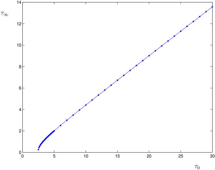
Figure 1: Plot of $\tau_{0}$ vs. $\tau_{\infty}$ for $n=1$ DF-vortex with $Q_{{\rm F1}}/{\cal T}_{3}=2$ and $R=\sqrt{2}$. At $\tau_{0}=2.46327$, $\tau_{\infty}\rightarrow 0$ which supports the logarithmically-increasing $\tau(r)$ at asymptotic region.

Inserting (3.28) into the various physical quantities (3.11), (3.13), (3.14)–(3.18), we read the followings. First, the radial electric field approaches rapidly a constant boundary value $|E_{r}(\infty)|=\sqrt{(1-E_{z}^{2})(1+\tau_{\infty}^{2})}\,$ ,

$$E_{r}^{2} \approx (1-E_{z}^{2})(1+\tau_{\infty}^{2})\left\{1-\frac{16{\cal T}_{3}^{2}R}{\tau_{\infty}Q_{\rm F1}^{2}}\left[1+\tau_{\infty}^{2}n^{2}\left(1+\frac{2\delta}{R}\right)\right]re^{-2\frac{\tau_{\infty}r+\delta}{R}}+\cdots\right\}.$$ (3.29)

Second, the leading terms of $\Pi^{z}$, $T^{t}_{t}$, $T^{r}_{r}$, $T^{z}_{z}$ are all proportional to $\Pi^{r}$ ($=Q_{{\rm F}1}/r$) and the subleading terms exponentially suppressed,

$$\Pi^{z2} \approx \frac{E_{z}^{2}(1+\tau_{\infty}^{2})}{1-E_{z}^{2}}\left(\frac{Q_{\rm F1}}{r}\right)^{2}\left[1+\frac{32{\cal T}_{3}^{2}}{Q_{\rm F1}^{2}}(1+\tau_{\infty}^{2}n^{2})r^{2}e^{-2\frac{\tau_{\infty}r+\delta}{R}}+\cdots\right],$$ (3.30)

$$T^{t}_{\;t} \approx -\sqrt{\frac{1+\tau_{\infty}^{2}}{1-E_{z}^{2}}}\,~{}\frac{|Q_{{\rm F1}}|}{r}\left[1+\frac{16{\cal T}_{3}^{2}}{Q_{\rm F1}^{2}}(1+\tau_{\infty}^{2}n^{2})r^{2}e^{-2\frac{\tau_{\infty}r+\delta}{R}}+\cdots\right],$$ (3.31)

$$T^{r}_{\;r} \approx -\sqrt{\frac{1-E_{z}^{2}}{1+\tau_{\infty}^{2}}}\,~{}\frac{|Q_{{\rm F1}}|}{r}\left\{1+\frac{8{\cal T}_{3}^{2}R}{\tau_{\infty}Q_{\rm F1}^{2}}\left[1+\tau_{\infty}^{2}n^{2}\left(1+\frac{2\delta}{R}\right)\right]re^{-2\frac{\tau_{\infty}r+\delta}{R}}+\cdots\right\},$$ (3.32)

$$T^{z}_{\;z} \approx -\sqrt{\frac{1+\tau_{\infty}^{2}}{1-E_{z}^{2}}}~{}\frac{|Q_{\rm F1}|}{r}\left[E_{z}^{2}+\frac{16{\cal T}_{3}^{2}}{Q_{\rm F1}^{2}}(1+\tau_{\infty}^{2}n^{2})r^{2}e^{-2\frac{\tau_{\infty}r+\delta}{R}}+\cdots\right].$$ (3.33)

Third, the angular components $j^{\theta}$ and $T^{\theta}_{\theta}$ exponentially decreasing so that, with (3.23) and (3.26), their shapes in $(r,\theta)$-plane look like a ring,

$$j^{\theta} \approx 16n\tilde{{\cal T}}_{3}^{2}\tau_{\infty}^{2}\sqrt{\frac{1+\tau_{\infty}^{2}}{1-E_{z}^{2}}}~{}\frac{|Q_{\rm F1}|}{r}e^{-2\frac{\tau_{\infty}r+\delta}{R}}+\cdots,$$ (3.34)

$$T^{\theta}_{\;\theta} \approx -16\tilde{{\cal T}}_{3}^{2}\sqrt{\frac{1+\tau_{\infty}^{2}}{1-E_{z}^{2}}}~{}\frac{r}{|Q_{\rm F1}|}e^{-2\frac{\tau_{\infty}r+\delta}{R}}+\cdots.$$ (3.35)

Here, we do not present the results of numerical analysis since the obtained configurations are exactly the same as those of D-strings [11] except for the fundamental-string charge density $\Pi^{z}$ in Fig. 2.

Figure 2: Plot of $\Pi^{z}(r)$ for the asymptotically-logarithmic (dashed line: $\tau_{0}=2.46327$) and asymptotically-linear (solid line: $\tau_{0}=6$) configurations of $\tau$. We set $n=1$, $Q_{{\rm F1}}/{\cal T}_{3}=2$, and $R=\sqrt{2}$ for superstring theory.

(ii) $\tau\sim\tau_{\infty}\ln r$ solution: If $\tau_{0}$ in the tachyon field near the origin (3.20) is sufficiently small, then this solution cannot reach $\tau(r=\infty)=\infty$. It means that there exists a critical value of $\tau_{0}$ which corresponds to $\tau^{\prime}(\infty)\rightarrow 0$ in (3.28), and it also requires a critical-charge density $(Q_{{\rm F}1}/{\cal T}_{3})^{2}=8/R^{2}$. In this limit, a natural asymptotic behavior of the tachyon amplitude is logarithmic, $\tau(r)\sim\tau_{\infty}{\rm ln}r$. If we try this configuration, the field equation (3.9) with (3.11) fixes the value of $\tau_{\infty}$ to $\tau_{\infty}=2R$, which leads the tachyon potential to a power-law decay, $V\approx 2/r^{2}$;

$$\tau(r)\approx 2R\,{\rm ln}r\left(1-2n^{2}R^{2}\frac{{\rm ln}r}{r^{2}}+\cdots\right).$$ (3.36)

Note that $\ln r$ is not well-defined at the entire region $(0\leq r\leq\infty)$, regularity of the obtained solution needs further mathematically-rigorous study. It turns out, in this case, that the radial component of the electric field $E_{r}$ (3.11) approaches a critical value at infinity with a power-law ${\cal O}(1/r^{2})$, $E_{r}^{2}(r=\infty)=1-E_{z}^{2}$,

$$E_{r}^{2}(r)\approx(1-E_{z}^{2})\left(1+\frac{2R^{2}}{r^{2}}+\cdots\right).$$ (3.37)

This looks similar to the case of the thick single topological BPS tachyon kink [20].

Inserting (3.36) into (3.13), (3.15), (3.16), and (3.18), we have again ${\cal O}(1/r)$ leading term in $\Pi^{z}$, $T^{t}_{\;t}$, $T^{r}_{\;r}$, and $T^{z}_{z}$,

$$\Pi^{z2} \approx \frac{E_{z}^{2}}{1-E_{z}^{2}}\left(\frac{Q_{\rm F1}}{r}\right)^{2}\left(1+\frac{6R^{2}}{r^{2}}+\cdots\right),$$ (3.38)

$$T^{t}_{\;t} \approx -\frac{1}{\sqrt{1-E_{z}^{2}}}\,\frac{|Q_{\rm F1}|}{r}\left(1+\frac{3R^{2}}{r^{2}}+\cdots\right),$$ (3.39)

$$T^{r}_{\;r} \approx -\sqrt{1-E_{z}^{2}}\,\frac{|Q_{\rm F1}|}{r}\left(1-\frac{R^{2}}{r^{2}}+\cdots\right),$$ (3.40)

$$T^{z}_{z} \approx -\frac{1}{\sqrt{1-E_{z}^{2}}}\frac{|Q_{\rm F1}|}{r}\left[E_{z}^{2}+(2+E_{z}^{2})\frac{R^{2}}{r^{2}}+\cdots\right].$$ (3.41)

The coefficients of the leading terms can be understood as the $\tau_{\infty}\rightarrow 0$ limit of (3.30)–(3.33) for the power-law solution. However, the subleading terms exhibit also a power-law behavior in (3.38)–(3.41), instead of the exponential decay in (3.30)–(3.33). This ${\cal O}(1/r)$ term makes its energy diverge linearly. On the other hand, the angular components of the current $j^{\theta}$ (3.14) and the pressure $T^{\theta}_{\;\theta}$ (3.17) have different behaviors for the leading terms. They have a power-law decay in this case while those for the linearly-growing tachyon have an exponential decay (3.36),

$$j^{\theta} \approx \frac{64n\,\tilde{{\cal T}_{3}^{2}}R^{2}}{\sqrt{1-E_{z}^{2}}~{}|Q_{\rm F1}|}\,\frac{(\ln r)^{2}}{r^{5}}+\cdots,$$ (3.42)

$$T^{\theta}_{\;\theta} \approx -\frac{16\tilde{{\cal T}}_{3}^{2}}{\sqrt{1-E_{z}^{2}}~{}|Q_{\rm F1}|}\,\frac{1}{r^{3}}+\cdots.$$ (3.43)

The numerical solution for the logarithmic tachyon amplitude connecting the origin and large $r$ is shown in Fig. 3-(a). We read $\tau_{0}$ as $\tau_{0}=2.46327$. The profile of the radial electric field $E_{r}$ decreases monotonically from a nonzero value larger than unity at the origin to unity at infinity as shown in Fig. 3-(b). The angular components of the current $j^{\theta}$ and the pressure $T^{\theta}_{\theta}$ have a ring shape connecting zeros at both boundaries, and $j^{\theta}$ is plotted in Fig. 3-(c). Since $\Pi^{z}$, $T^{t}_{t}$, $T^{r}_{r}$, and $T^{z}_{z}$ behave in a similar way, we only draw the figure of $\Pi^{z}$ which has ${\cal O}(1/r)$ singularity at the origin and decreases monotonically to zero as shown in Fig. 2. Both the power-law solution (3.28) and the logarithmic solution (3.36) share similar shapes for $\Pi^{z}$ as are given by the solid and dashed lines in Fig. 2.

Figure 3: (a) Plot of $\tau(r)$ with logarithmic behavior for large $r$, (b) Plot of $E_{r}(r)$, and (c) Plot of $j^{\theta}$. We set $n=1$, $Q_{{\rm F1}}/{\cal T}_{3}=2$, $R=\sqrt{2}$, and $\tau_{0}=2.46327$.

The leading linear divergence in the energy of the obtained DF-string configurations per unit length along the $z$-direction can be read off from (3.31) and (3.39),

$$\frac{E}{\int dz}=\int_{0}^{R_{{\rm IR}}}drrd\theta\,T_{tt}=2\pi\sqrt{\frac{1+\tau_{\infty}^{2}}{1-E_{z}^{2}}}\,|Q_{{\rm F1}}|R_{{\rm IR}}+({\rm finite}).$$ (3.44)

Since the divergent part is linearly proportional to the fundamental-string charge density at the origin, a possible source of this infra-red divergence is different from the familiar nature of logarithmically divergent energy of the global vortex. For a given fundamental-string charge density $Q_{{\rm F1}}$, the energy spectrum of each solution is classified by $\tau_{\infty}$. In that sense, the logarithmic solution with $\tau_{\infty}=0$ in (3.44) is the minimum energy solution of the D- or DF-strings.

If we take the limit of vanishing fundamental-string charge density $Q_{{\rm F}1}\rightarrow 0$, the first terms proportional to $Q_{{\rm F}1}^{2}$ in $T^{t}_{\;t}$, (3.24) and (3.31) approach zero for the linearly-growing solution (3.28). From behavior of the second $Q_{{\rm F}1}$-independent terms in (3.24) and (3.31), we may read the limit of $\delta$-function like configuration in the limit of $\tau_{\infty}\rightarrow\infty$. This phenomenon is consistent with the existence of singular vortex solution in the absence of $Q_{{\rm F}1}^{2}$ [3]. When the electric field $E_{z}$ approaches critical value, various densities including $\Pi^{z}$ (3.13), $T^{t}_{\;t}$ (3.15), $T^{z}_{\;z}$ (3.18), $j^{\theta}$ (3.14), and $T^{\theta}_{\;\theta}$ diverge with the finite fundamental-string charge density $Q_{{\rm F}1}$, but $E_{r}$ (3.11) and $T^{r}_{\;r}$ (3.16) go to zero. These can easily be checked also by the expanded expressions given in this subsection. This singularity was expected from the beginning if we see the expression of determinant (3.5) in the action (2.1).

There is another coupling to the bulk RR fields given by the Wess-Zumino term, and, for the global DF-strings from D$3{\bar{\rm D}}3$ [1, 2, 3, 21], it is

$$S_{\rm WZ} = \mu~{}{\rm Str}\int_{\Sigma_{4}}C_{\rm RR}\wedge{\rm exp}\left(\begin{array}[]{cc}F^{1}-T\bar{T}&i^{3/2}~{}\partial T\\ -i^{3/2}~{}\partial\overline{T}&F^{2}-\bar{T}T\end{array}\right)$$ (3.47)

$$= -n\mu\int_{\Sigma_{4}}\frac{de^{-\tau^{2}}}{dr}\left(C_{\rm RR}^{(1)}\wedge dr\wedge d\theta+\frac{E_{z}}{3}C_{\rm RR}^{(-1)}\wedge dt\wedge dr\wedge d\theta\wedge dz\right),$$ (3.48)

$$\propto n,$$ (3.49)

where $\mu$ is a real constant and the supertrace ${\rm Str}$ is defined to be a trace with $\sigma_{3}$ inserted. The first term in (3.48) means the charge of a D1-brane stretched along the $z$-axis, which is proportional to the vorticity $n$. Thus the charge density of the D1-brane per unit length is identified as the topological charge of which current density is defined by

$$j_{{\rm D}1}^{\mu}=\frac{{\bar{T}}\partial^{\mu}T-T\partial^{\mu}{\bar{T}}}{4\pi i{\bar{T}}T}.$$ (3.50)

Although the second term proportional to both $n$ and $E_{z}$ in (3.48) implies an (Minkowski) instanton charge, its possible physical meaning will be discussed in the next subsection. In addition to the D1 charge (3.50), the stringy object of interest carries the charge of fundamental strings along the $z$-axis, which is denoted by the localized electric flux $\Pi^{z}$ (3.13). Since the point charge $Q_{{\rm F}1}$ (3.8) at $r=0$ is nothing but the background charge distribution of fundamental strings coming from a transverse direction, and is ending on a point along the $z$-axis, the stringy object carrying the vortex charge $n$ and the localized electric flux $\Pi^{z}$ is identified as a DF-string or a $(p,q)$-string (composite of D1F1) from D3${\bar{\rm D}}3$ system with fundamental strings. What we obtained is summarized schematically in Fig. 4. If the early Universe involved a D3${\bar{\rm D}}3$, the obtained DF-string can remain as a cosmic fossil named as the cosmic global DF-string.

Figure 4: D3 and ${\bar{\rm D}}3$ with fundamental strings represented by $\Pi^{r}(r)$. Straight DF-strings represented by $n$ and $\Pi^{z}$ are formed.

3.2 Local DF-strings

When the gauge field $C_{\mu}$ (3.3) is turned on, the character of DF-strings becomes local. In usual local field theories, e.g., the Abelian-Higgs model, a role of the gauge field is to make energy of the local vortex (energy density of the vortex-string per unit length along the string) finite by trimming the logarithmically-divergent energy of the global vortex [5]. This phenomenon was not observed in D-vortices from D2${\bar{\rm D}}$2 system with fundamental strings; the energy of the D-vortex is linearly-divergent, but its source is fundamental string charges [11]. Although this sort of energy-trimming seems unlikely also for local DF-strings of our interest, we investigate the existence and the property of local DF-strings in this subsection.

Since the inclusion of the gauge field $C_{\theta}$ (3.3) requires the analysis of the coupled equations (3.9)–(3.10), we need boundary conditions for the gauge field in addition to those for the tachyon (3.19),

$$C_{\theta}(0)=0,\qquad C_{\theta}(\infty)=\frac{n}{2}.$$ (3.51)

From now on, we examine the differential equations (3.9)–(3.10) and the expressions (3.11) and (3.13) for $E_{r}$ and $\Pi^{z}$, and find local DF-string solutions satisfying the boundary conditions (3.19) and (3.51).

Near the origin, the power-series expansion of $\tau(r)$ and $C_{\theta}(r)$ for DF-string solutions gives

$$\tau(r)\approx\left\{\begin{array}[]{ll}\tau_{0}r\left[1-\frac{{\cal T}_{3}^{2}(1+\tau_{0}^{2})^{2}}{5Q_{\rm F1}^{2}R^{2}}r^{4}+\cdots\right],&n=1\\ \tau_{0}r\left[1+\frac{(n^{2}-1)\alpha}{6}r^{2}+\cdots\right],&n\geq 2\end{array}\right.$$ (3.52)

$$C_{\theta}(r)\approx C_{0}r^{3}\left[1-\frac{3+\tau_{0}^{2}n^{2}(5-2n^{2})}{10(1+\tau_{0}^{2}n^{2})}\alpha r^{2}+\cdots\right],\qquad n\geq 1$$ (3.53)

where $\alpha$ is

$$\alpha=\frac{1}{(1+\tau_{0}^{2}n^{2})^{2}}\left[\frac{4{\cal T}_{3}^{2}}{Q_{\rm F1}^{2}}(1+\tau_{0}^{2})(1+\tau_{0}^{2}n^{2})^{2}-9C_{0}^{2}\right].$$ (3.54)

For the local DF-strings with unit vorticity, the increasing rate of the tachyon amplitude (3.52) is not affected by $C_{0}$ up to the second order. On the other hand, the signature in front of $9C_{0}^{2}$ in (3.54) is opposite to that of the first term which is proportional to ${\cal T}_{3}^{2}/Q_{{\rm F}1}^{2}$, so the increasing rate of the tachyon amplitude (3.52) becomes smaller for local DF-strings.

Inserting the expansions (3.52)–(3.53) into the radial electric field $E_{r}$ (3.11) and the fundamental-string charge density $\Pi^{z}$ (3.13), we have a nonzero value, $(1-E_{z}^{2})(1+\tau_{0}^{2})$, for $E_{r}$ and singular $|\Pi^{z}|$ at the origin

$$E_{r}^{2}(r) \approx (1-E_{z}^{2})(1+\tau_{0}^{2})(1-\alpha r^{2}+\cdots),$$ (3.55)

$$\Pi^{z2} \approx \frac{E_{z}^{2}(1+\tau_{0}^{2})}{(1-E_{z}^{2})}\left(\frac{Q_{\rm F1}}{r}\right)^{2}\left(1-\beta r^{2}+\cdots\right),$$ (3.56)

where $\beta$ is

$$\beta=-\frac{1}{(1+\tau_{0}^{2}n^{2})^{2}}\left[\frac{4{\cal T}_{3}^{2}}{Q_{\rm F1}^{2}}(1+\tau_{0}^{2}(2n^{2}-1))(1+\tau_{0}^{2}n^{2})^{2}+9C_{0}^{2}\right].$$ (3.57)

The current density (3.14) again increases from zero

$$j^{\theta}\approx\sqrt{\frac{1-E_{z}^{2}}{1+\tau_{0}^{2}}}~{}\tau_{0}^{2}n|Q_{\rm F1}|\alpha r+\cdots,$$ (3.58)

and nonvanishing components of the energy-momentum density (3.15)–(3.18) show the following behavior which is similar to the case of global DF-strings (3.24)–(3.27)

$$T^{t}_{\;t} \approx -\sqrt{\frac{1+\tau_{0}^{2}}{1-E_{z}^{2}}}~{}\frac{|Q_{\rm F1}|}{r}\left(1-\frac{\beta}{2}r^{2}+\cdots\right),$$ (3.59)

$$T^{r}_{\;r} \approx -\sqrt{\frac{1-E_{z}^{2}}{1+\tau_{0}^{2}}}~{}\frac{|Q_{\rm F1}|}{r}\left(1+\frac{\alpha}{2}r^{2}+\cdots\right),$$ (3.60)

$$T^{\theta}_{\;\theta} \approx -\sqrt{\frac{1-E_{z}^{2}}{1+\tau_{0}^{2}}}\,|Q_{\rm F1}|\alpha r+\cdots,$$ (3.61)

$$T^{z}_{\;z} \approx -E_{z}^{2}\sqrt{\frac{1+\tau_{0}^{2}}{1-E_{z}^{2}}}~{}\frac{|Q_{\rm F1}|}{r}\left\{1-\left[\frac{\alpha}{2}-\frac{4(1+\tau_{0}^{2}n^{2})}{E_{z}^{2}}\frac{{\cal T}_{3}^{2}}{Q_{{\rm F}1}^{2}}\right]r^{2}+\cdots\right\}.$$ (3.62)

The near-origin behavior of the local DF-string solutions is parameterized smoothly by $\tau_{0}$ in (3.52) and $C_{0}$ in (3.53). At asymptotic region, the tachyon amplitude of every local DF-string will be proven to approach universally the vacuum, but the approaching behavior is sorted into two; (i) linear divergence $\tau\sim\tau_{\infty}r$ and (ii) logarithmic divergence $\tau\sim\tau_{\infty}\ln r$, as were for the global DF-strings in the previous subsection. We analyze the DF-string solutions with the linearly-divergent $\tau$ and the logarithmically-divergent $\tau$ separately in what follows.

(i) $\tau\sim\tau_{\infty}r$ solutions: If we examine carefully the coupled differential equations (3.9)–(3.10), the leading asymptotic behavior of the tachyon amplitude is either linearly-growing or logarithmically-growing. First, we consider the linearly-growing case. The subleading term of the tachyon amplitude is decreasing exponentially

$$\tau(r) \approx \tau_{\infty}r+\delta-\frac{4{\cal T}_{3}^{2}R(1+\tau_{\infty}^{2})}{\tau_{\infty}^{2}Q_{\rm F1}^{2}}~{}r^{2}e^{-2\frac{\tau_{\infty}r+\delta}{R}}+\cdots,$$ (3.63)

where $\tau_{\infty}$ and $\delta$ are undetermined constants which are governed by the behavior near the origin. For the gauge field $C_{\theta}$, we consider small $\delta C_{\theta}$ at the asymptotic region,

$$C_{\theta}(r) \approx \frac{n}{2}+\delta C_{\theta}.$$ (3.64)

Substituting this into the equation for the gauge field, we obtain a linear equation,

$$M(t)\frac{d^{2}\delta C_{\theta}}{dt^{2}}=-\frac{d}{d\delta C_{\theta}}U(\delta C_{\theta}),\qquad t=\kappa r^{3},\quad\left(\kappa=\frac{4{\cal T}_{p}\tau_{\infty}}{3|Q_{\rm F1}|}\sqrt{1+\tau_{\infty}^{2}}e^{-\delta/R}\right),$$ (3.65)

where $M(t)=e^{2\tau_{\infty}t^{1/3}/(R\kappa^{1/3})}$ and $U=-(\delta C_{\theta})^{2}/2$. If we identify $\delta C_{\theta}$ as a one-dimensional position of a hypothetical particle, Eq. (3.65) is interpreted as a Newtonian equation with a variable mass $M(t)$ and a conservative potential $U(\delta C_{\theta})$. The nontrivial analytic solution satisfying $\delta C_{\theta}(r=\infty)=0$ is not known yet, but the existence of such solution can easily be read from the properties of $U(\delta C_{\theta})$; max[$U(\delta C_{\theta})$]=0 at $\delta C_{\theta}=0$ and min[$U(\delta C_{\theta})]=-\infty$ at $\delta C_{\theta}=\pm\infty$.

With the asymptotic behavior of the tachyon amplitude (3.63) and the gauge field (3.64), the radial electric field approaches its boundary value exponentially,

$$E_{r}^{2}(r) \approx (1-E_{z}^{2})(1+\tau_{\infty}^{2})\left(1-\frac{16{\cal T}_{3}^{2}R}{\tau_{\infty}Q_{\rm F1}^{2}}re^{-2\frac{\tau_{\infty}r+\delta}{R}}+\cdots\right),$$ (3.66)

and the U(1) current and the angular component of the energy-momentum tensor decay exponentially to zero,

$$j^{\theta} \approx -32{\tilde{\cal T}}_{3}^{2}\tau_{\infty}^{2}\sqrt{\frac{1+\tau_{\infty}^{2}}{1-E_{z}^{2}}}~{}\frac{r}{|Q_{\rm F1}|}e^{-2\frac{\tau_{\infty}r+\delta}{R}}\delta C_{\theta},$$ (3.67)

$$T^{\theta}_{\;\theta} \approx -16\tilde{{\cal T}}_{3}^{2}\sqrt{\frac{1+\tau_{\infty}^{2}}{1-E_{z}^{2}}}~{}\frac{r}{|Q_{\rm F1}|}e^{-2\frac{\tau_{\infty}r+\delta}{R}}+\cdots.$$ (3.68)

As it was the case of global DF-strings in the previous subsection, the leading terms of $\Pi^{z}$, $T^{t}_{\;t}$, $T^{r}_{\;r}$, and $T^{z}_{\;z}$ are commonly proportional to $Q_{\rm F1}/r$ but the subleading terms decrease exponentially,

$$\Pi^{z2} \approx \frac{E_{z}^{2}(1+\tau_{\infty}^{2})}{1-E_{z}^{2}}\left(\frac{Q_{\rm F1}}{r}\right)^{2}\left(1+\frac{32{\cal T}_{3}^{2}}{Q_{\rm F1}^{2}}r^{2}e^{-2\frac{\tau_{\infty}r+\delta}{R}}+\cdots\right),$$ (3.69)

$$T^{t}_{\;t} \approx -\sqrt{\frac{1+\tau_{\infty}^{2}}{1-E_{z}^{2}}}~{}\frac{|Q_{\rm F1}|}{r}\left(1+\frac{16{\cal T}_{3}^{2}}{Q_{\rm F1}^{2}}~{}r^{2}e^{-2\frac{\tau_{\infty}r+\delta}{R}}+\cdots\right),$$ (3.70)

$$T^{r}_{\;r} \approx -\sqrt{\frac{1-E_{z}^{2}}{1+\tau_{\infty}^{2}}}~{}\frac{|Q_{\rm F1}|}{r}\left(1+\frac{8{\cal T}_{3}^{2}R}{\tau_{\infty}Q_{\rm F1}^{2}}re^{-2\frac{\tau_{\infty}r+\delta}{R}}+\cdots\right),$$ (3.71)

$$T^{z}_{\;z} \approx -\sqrt{\frac{1+\tau_{\infty}^{2}}{1-E_{z}^{2}}}~{}\frac{|Q_{\rm F1}|}{r}\left(E_{z}^{2}+\frac{16{\cal T}_{3}^{2}}{Q_{\rm F1}^{2}}r^{2}e^{-2\frac{\tau_{\infty}r+\delta}{R}}+\cdots\right).$$ (3.72)

Note that the leading long-range terms of local DF-strings are the same as those of global DF-strings, and that the limiting behaviors for the large, or small $Q_{{\rm F}1}^{2}$, and for the critical electric field $|E_{z}|\rightarrow 1$, are also the same.

(ii) $\tau\sim\tau_{\infty}\ln r$ solutions: Lastly let us discuss logarithmic $\tau$-solution of the local DF-string. For sufficiently large $r$, the leading logarithmic term has the same coefficient with the global DF-string (3.36), but the subleading term does not contain logarithmic term;

$$\tau(r) \approx 2R~{}{\rm ln}r-\frac{4R^{3}}{r^{2}}+\cdots.$$ (3.73)

As we observed in the global string case, the first subleading term of $E_{r}$ in (3.37) is governed only by the leading term of the tachyon amplitude in (3.36). Therefore, the expansion for the logarithmic $\tau$-solution is the same for the local string. If we try to get the asymptotic solution of the gauge field $C_{\theta}$ similarly to the case of linearly-growing solution (3.64), the linearized equation for $\delta C_{\theta}$ is

$$\frac{d}{dr}\left(\frac{\delta C_{\theta}^{\prime}}{r^{2}}\right)\approx 32R^{4}\frac{({\rm ln}r)^{2}}{r^{4}}\delta C_{\theta}.$$ (3.74)

We find a solution which decreases rapidly to zero,

$$\delta C_{\theta}(r)\approx C_{1}\frac{r^{\frac{3}{2}}}{\sqrt{\ln r}}\,{\rm WhittakerW}\left(-\frac{9}{128}\frac{\sqrt{2}}{R},\,\frac{1}{4},\,4\sqrt{2}R(\ln r)^{2}\right),$$ (3.75)

where $C_{1}$ is an integration constant which is to be set by the boundary conditions at the asymptotic. As shown in Fig. 5, the gauge field $C_{\theta}$ (the dashed line) reaches its boundary value $n/2$ rapidly and the tachyon amplitude $\tau$ (the solid line) grows logarithmically. Due to the mixture of slowly-growing and rapidly-growing functional behaviors for single numerical analysis, the results of numerical work need further improvement for this logarithmic case.

Figure 5: For $n=1$ and $R=\sqrt{2}$, profile of the tachyon amplitude $\tau(r)$ by the solid line ($\tau_{0}=2.4489$) and that of the gauge field $C_{\theta}(r)$ by the dashed line ($C_{0}=4.5733$).

This rapidly-decreasing behavior of the gauge field $C_{\theta}$ affects that of the U(1) current (3.14), but does not appear in the radial pressure (3.16) up to the leading order,

$$j^{\theta} \approx -\frac{128\,\tilde{{\cal T}_{3}^{2}}R^{2}}{\sqrt{1-E_{z}^{2}}~{}|Q_{\rm F1}|}\,\frac{(\ln r)^{2}}{r^{5}}\delta C_{\theta}+\cdots,$$ (3.76)

$$T^{\theta}_{\;\theta} \approx -\frac{16\tilde{{\cal T}}_{3}^{2}}{\sqrt{1-E_{z}^{2}}~{}|Q_{\rm F1}|}\,\frac{1}{r^{3}}+\cdots.$$ (3.77)

Similar to $E_{r}$, all the components of the energy-momentum tensor and the $z$-component of the electric flux density for the local DF-string have the same functional forms with those of the corresponding components of the global DF-string up to the second order terms. Therefore, the leading energy density of the local DF-string for the logarithmically-growing tachyon amplitude shares that of the local DF-string for the linearly-growing tachyon amplitude and that of the global strings. It means that the discussion on the energy of the global DF-strings can also be applied to that of the local DF-strings; the role of the gauge field $C_{\theta}$ in localizing the energy of the string is negligible, which is very different from that in the case of Nielsen-Olesen vortex-string in the Abelian-Higgs model.

Due to the gauge field $C_{\theta}$, the Wess-Zumino term of D$3{\bar{\rm D}}3$ describing coupling to the bulk RR fields becomes slightly different from that of the global DF-strings [1, 2, 3, 21],

$$S_{\rm WZ} = \mu~{}{\rm Str}\int_{\Sigma_{4}}C_{\rm RR}\wedge{\rm exp}\left(\begin{array}[]{cc}F^{1}-T\bar{T}&i^{3/2}~{}DT\\ -i^{3/2}~{}\overline{DT}&F^{2}-\bar{T}T\end{array}\right)$$ (3.81)

$$= 2\mu\int_{\Sigma_{4}}\left\{\frac{d}{dr}\left[e^{-\tau^{2}}\left(C_{\theta}-\frac{n}{2}\right)\right]\left(C_{\rm RR}^{(1)}+\frac{E_{z}}{3}C_{\rm RR}^{(-1)}\wedge dt\wedge dz\right)\wedge dr\wedge d\theta\right.$$

$$\hskip 42.67912pt\left.-\frac{1}{3}E_{z}C_{r\theta}C_{\rm RR}^{(-1)}\wedge dt\wedge dr\wedge d\theta\wedge dz\right\}.$$

The term of $C_{\rm RR}^{(1)}$ coupling is proportional to the vorticity $n$ so that the local DF-string carries the quantized magnetic flux as a D1 charge density per unit length along the $z$-axis,

$$\Phi=\int_{0}^{\infty}dr\int_{0}^{2\pi}d\theta\,C_{r\theta}=\pi n.$$ (3.82)

Note that the second term in (3.81) tells us that $C_{\rm RR}^{(-1)}$ coupling is nothing but an axion coupling. Since we have additionally the fundamental-string charge density $\Pi^{z}$ localized along the string direction (the $z$-axis in our case), the obtained stringy objects are local DF-strings, or local $(p,q)$-strings from D3${\bar{\rm D}}$3 system with fundamental strings.

4 Conclusions

The system of D3${\bar{\rm D}}3$ with fundamental strings has been considered in the coincidence limit of a brane and an anti-brane. In the scheme of effective field theory, it is described by the DBI type effective action of a complex tachyon field and U(1)$\times$U(1) gauge fields. The runaway tachyon potential has U(1) vacua at an infinite tachyon amplitude, which supports topological vortex-strings of codimension-two. Specifically, we study straight string solutions by examining field equations.

The topological charge of the string represented by vorticity is interpreted as the RR-charge density of D-string (D1-brane). (See the circles in Fig. 4.) Introduction of the radial DBI electric field coupled nonminimally to the tachyon is indispensable to obtain a thick D-string, which implies that background fundamental strings live in an extra-dimension with a fluid form and end at each vortex-string origin. (See the radial arrows in Fig. 4.)

According to asymptotic behavior of the tachyon amplitude at infinity, we obtained either linearly-growing tachyon configurations, or a newly-found lograrithmically-growing tachyon configuration which represents the minimum energy configuration. We additionally turn on the constant DBI electric field parallel to the string. Then its conjugate momentum density is localized along the string. (See the straight arrows along the $z$-direction in Fig. 4.) This confined electric flux density tells us that the stringy object of interest carries a fundamental string charge density, so we find it a DF-string (or a $(p,q)$-string). Lastly the nonvanishing gauge field coupled minimally to the tachyon replaces the global DF-string by a local DF-string carrying a quantized magnetic flux density as a D1 charge density.

Now that we have global and local, D- and DF-strings as soliton solutions in the context of effective field theory [11], the future tasks to construct a viable cosmic superstring become more tractable. Dynamical issues [7, 8, 9] involve (i) head-on collision of two D-vortices for checking the intercommuting (reconnecting) property of two D-strings, (ii) collision of two DF-strings leading to a tree structure composed of a pair of trilinear vertices, which is to form a cosmic DF-string network [22], and (iii) the stability of long macroscopic D- and DF-strings.

On cosmological aspects, we would gravitate the obtained static stringy defects and see the resultant spacetime structure. This may provide a basis to tackle the possibility of observing its effect astrophysically including viable density fluctuations and quintessence [23]. Inclusion of time-dependence is also important to understand how the D- and DF-strings are generated, and whether or not they survive during the inflationary era induced by the separation of D3 and ${\bar{\rm D}}3$. To lower the scale from the fundamental string scale to a scale to pass observational tests such as the cosmic microwave background, the pulsar timing, and the gravitational radiation, it is also intriguing to take into account the D- and DF-strings obtained in the background of various string (inspired) models [24].

References

- [1] P. Kraus and F. Larsen, “Boundary string field theory of the DD-bar system,” Phys. Rev. D 63, 106004 (2001) [arXiv:hep-th/0012198]; T. Takayanagi, S. Terashima and T. Uesugi, “Brane-antibrane action from boundary string field theory,” JHEP 0103, 019 (2001) [arXiv:hep-th/0012210].
- [2] N. T. Jones and S. H. H. Tye, “An improved brane anti-brane action from boundary superstring field theory and multi-vortex solutions,” JHEP 0301, 012 (2003) [arXiv:hep-th/0211180].
- [3] A. Sen, “Dirac-Born-Infeld action on the tachyon kink and vortex,” Phys. Rev. D 68, 066008 (2003) [arXiv:hep-th/0303057].
- [4] G. R. Dvali and S. H. H. Tye, “Brane inflation,” Phys. Lett. B 450, 72 (1999) [arXiv:hep-ph/9812483]; G. R. Dvali, Q. Shafi and S. Solganik, “D-brane inflation,” arXiv:hep-th/0105203; C. P. Burgess, M. Majumdar, D. Nolte, F. Quevedo, G. Rajesh and R. J. Zhang, “The inflationary brane-antibrane universe,” JHEP 0107, 047 (2001) [arXiv:hep-th/0105204]; J. Garcia-Bellido, R. Rabadan and F. Zamora, “Inflationary scenarios from branes at angles,” JHEP 0201, 036 (2002) [arXiv:hep-th/0112147]; S. H. S. Alexander, “Inflation from D - anti-D brane annihilation,” Phys. Rev. D 65, 023507 (2002) [arXiv:hep-th/0105032]; E. Halyo, “Inflation from rotation,” arXiv:hep-ph/0105341; G. Shiu and S. H. H. Tye, “Some aspects of brane inflation,” Phys. Lett. B 516, 421 (2001) [arXiv:hep-th/0106274]; C. Herdeiro, S. Hirano and R. Kallosh, “String theory and hybrid inflation / acceleration,” JHEP 0112, 027 (2001) [arXiv:hep-th/0110271]; B. s. Kyae and Q. Shafi, “Branes and inflationary cosmology,” Phys. Lett. B 526, 379 (2002) [arXiv:hep-ph/0111101]; R. Blumenhagen, B. Kors, D. Lust and T. Ott, “Hybrid inflation in intersecting brane worlds,” Nucl. Phys. B 641, 235 (2002) [arXiv:hep-th/0202124]; N. Jones, H. Stoica and S. H. H. Tye, “Brane interaction as the origin of inflation,” JHEP 0207, 051 (2002) [arXiv:hep-th/0203163].
- [5] A. Vilenkin and E. P. S. Shellard, Cosmic Strings and Other Topological Defects, (Cambridge University Press, 1984).
- [6] T. W. B. Kibble, “Cosmic strings reborn?,” arXiv:astro-ph/0410073; A. Vilenkin, “Cosmic strings: Progress and problems,” arXiv:hep-th/0508135.
- [7] G. Dvali and A. Vilenkin, “Formation and evolution of cosmic D-strings,” JCAP 0403, 010 (2004) [arXiv:hep-th/0312007].
- [8] E. J. Copeland, R. C. Myers and J. Polchinski, “Cosmic F- and D-strings,” JHEP 0406, 013 (2004) [arXiv:hep-th/0312067].
- [9] L. Leblond and S. H. H. Tye, “Stability of D1-strings inside a D3-brane,” JHEP 0403, 055 (2004) [arXiv:hep-th/0402072]; T. Matsuda, “String production after angled brane inflation,” Phys. Rev. D 70, 023502 (2004) [arXiv:hep-ph/0403092]; M. G. Jackson, N. T. Jones and J. Polchinski, “Collisions of cosmic F- and D-strings,” arXiv:hep-th/0405229; K. Dasgupta, J. P. Hsu, R. Kallosh, A. Linde and M. Zagermann, “D3/D7 brane inflation and semilocal strings,” JHEP 0408, 030 (2004) [arXiv:hep-th/0405247]; A. Achucarro and J. Urrestilla, “F-term strings in the Bogomolnyi limit are also BPS states,” JHEP 0408, 050 (2004) [arXiv:hep-th/0407193]; T. Damour and A. Vilenkin, “Gravitational radiation from cosmic (super)strings: Bursts, stochastic background, and observational windows,” Phys. Rev. D 71, 063510 (2005) [arXiv:hep-th/0410222]; N. Barnaby, A. Berndsen, J. M. Cline and H. Stoica, “Overproduction of cosmic superstrings,” JHEP 0506, 075 (2005) [arXiv:hep-th/0412095]; H. Firouzjahi and S. H. Tye, “Brane inflation and cosmic string tension in superstring theory,” JCAP 0503, 009 (2005) [arXiv:hep-th/0501099]; S. H. Tye, I. Wasserman and M. Wyman, “Scaling of multi-tension cosmic superstring networks,” Phys. Rev. D 71, 103508 (2005) [Erratum-ibid. D 71, 129906 (2005)] [arXiv:astro-ph/0503506]; E. J. Copeland and P. M. Saffin, “On the evolution of cosmic-superstring networks,” arXiv:hep-th/0505110; A. C. Davis and K. Dimopoulos, “Cosmic superstrings and primordial magnetogenesis,” Phys. Rev. D 72, 043517 (2005) [arXiv:hep-ph/0505242]; P. M. Saffin, “A practical model for cosmic (p,q) superstrings,” JHEP 0509, 011 (2005) [arXiv:hep-th/0506138]; E. I. Buchbinder, “On Open Membranes, Cosmic Strings and Moduli Stabilization,” Nucl. Phys. B 728, 207 (2005) [arXiv:hep-th/0507164]; B. Shlaer and M. Wyman, “Cosmic superstring gravitational lensing phenomena: Predictions for networks of (p,q) strings,” arXiv:hep-th/0509177.
- [10] J. J. Blanco-Pillado, G. Dvali and M. Redi, “Cosmic D-strings as axionic D-term strings,” arXiv:hep-th/0505172;
- [11] Y. Kim, B. Kyae and J. Lee, “Global and local D-vortices,” JHEP 0510, 002 (2005) [arXiv:hep-th/0508027].
- [12] For a review, see J. Polchinski, “Introduction to cosmic F- and D-strings,” arXiv:hep-th/0412244.
- [13] E. Witten, “Cosmic Superstrings,” Phys. Lett. B 153, 243 (1985).
- [14] N. T. Jones, L. Leblond and S. H. H. Tye, “Adding a brane to the brane anti-brane action in BSFT,” JHEP 0310, 002 (2003) [arXiv:hep-th/0307086].
- [15] A. Sen “Non-BPS states and branes in string theory,” arXiv:hep-th/9904207.
- [16] A. Sen, “Universality of the tachyon potential,” JHEP 9912, 027 (1999) [arXiv:hep-th/9911116].
- [17] A. Sen, “Field theory of tachyon matter,” Mod. Phys. Lett. A 17, 1797 (2002) [arXiv:hep-th/0204143].
- [18] D. Kutasov and V. Niarchos, “Tachyon effective actions in open string theory,” Nucl. Phys. B 666, 56 (2003) [arXiv:hep-th/0304045].
- [19] A. Buchel, P. Langfelder and J. Walcher, “Does the tachyon matter?,” Annals Phys. 302, 78 (2002) [arXiv:hep-th/0207235]; C. Kim, H. B. Kim, Y. Kim and O-K. Kwon, “Electromagnetic string fluid in rolling tachyon,” JHEP 0303, 008 (2003) [arXiv:hep-th/0301076]; F. Leblond and A. W. Peet, “SD-brane gravity fields and rolling tachyons,” JHEP 0304, 048 (2003) [arXiv:hep-th/0303035].
- [20] C. Kim, Y. Kim and C. O. Lee, “Tachyon kinks,” JHEP 0305, 020 (2003) [arXiv:hep-th/0304180]; A. Sen, “Open and closed strings from unstable D-branes,” Phys. Rev. D 68, 106003 (2003) [arXiv:hep-th/0305011]; C. Kim, Y. Kim, O-K. Kwon and C. O. Lee, “Tachyon kinks on unstable Dp-branes,” JHEP 0311, 034 (2003) [arXiv:hep-th/0305092].
- [21] C. Kennedy and A. Wilkins, “Ramond-Ramond couplings on brane-antibrane systems,” Phys. Lett. B 464, 206 (1999) [arXiv:hep-th/9905195];
- [22] K. Hashimoto and S. Nagaoka, “Realization of brane descent relations in effective theories,” Phys. Rev. D 66, 026001 (2002) [arXiv:hep-th/0202079].
- [23] I. Cho and A. Vilenkin, “Vacuum defects without a vacuum,” Phys. Rev. D 59, 021701 (1999) [arXiv:hep-th/9808090]; I. Cho and A. Vilenkin, “Gravitational field of vacuumless defects,” Phys. Rev. D 59, 063510 (1999) [arXiv:gr-qc/9810049].
- [24] S. Sarangi and S. H. H. Tye, “Cosmic string production towards the end of brane inflation,” Phys. Lett. B 536, 185 (2002) [arXiv:hep-th/0204074]; S. Kachru, R. Kallosh, A. Linde, J. Maldacena, L. McAllister and S. P. Trivedi, “Towards inflation in string theory,” JCAP 0310, 013 (2003) [arXiv:hep-th/0308055]; K. Becker, M. Becker and A. Krause, “Heterotic cosmic strings,” arXiv:hep-th/0510066.