Imaginary Sources: Completeness Conjecture and Charges

Abstract:

While in string theory the subject of sources in imaginary time has received some attention, we demonstrate the power of imaginary sources by proving that they constitute in several field theories a complete basis for all smooth and time dependent source free solutions. These proofs promote the study of imaginary sources to a new and crucial viewpoint for understanding time dependent backgrounds. From our field theory examples we further propose a completeness conjecture that every regular solution to a field equation of motion has a corresponding imaginary source configuration. We define charges for spacelike sources and show their compatibility with the usual charge definition for timelike sources. Many new non-singular time dependent field theory solutions are discussed, including Wick rotations of abelian instantons which demonstrate a close relationship between electric-magnetic duals and analytic continuation.

1 Imaginary Sources

1.1 General concept

Time-dependent backgrounds are a big issue for reconciling string theory with cosmology, which has been a driving force for their study in recent years. A time-dependent boundary state Sen described as rolling tachyon [1] was obtained by a Wick rotation, and since boundary states generically act as sources for closed strings including gravity, this necessarily introduces [2, 3, 4, 5, 6] a notion of sources at imaginary spacetime, which we call imaginary sources in short. This concept has been used in various situations implicitly, for example in Wick rotation of gravity solutions, etc. In this paper, we study how the concept of imaginary sources is general and fundamental.

Inserting sources in imaginary spacetime in various field theories create many time-dependent classical solutions. While discovering new solutions is interesting, the question is how much about time dependent backgrounds do we expect to learn from their study. As a general remark, first of all, the fact that these solutions do have sources under analytic continuation is already fascinating, and more importantly generalizes a host of previous sources such as black holes, electrons, branes, strings to imaginary cases. Because of the plethora of discussions of these objects, the fact that their imaginary versions are consistent should give rise to much interesting study.

A priori time-dependent solutions obtained by the analytic continuation of sources seem to some degree artificial. However, we claim that it is opposite: sources in imaginary spacetimes have full flexibility in reproducing all the regular solutions to homogeneous equations of motion, and will give a proof of this completeness conjecture for several field theories.

Once assuming that this conjecture is true for all field theories, one important question is how we can recover the information of the imaginary sources from given time-dependent solutions. A step toward answering this question will be given as a new definition of charges for time-dependent configurations.

Sources at imaginary spacetime

Let us first review the basic properties of analytic continuation and introduce the concept of imaginary sources. To describe a physical system we take as our starting point a set of real differential equations with arbitrary number of derivatives with respect to $\{x_{i}\}$ for $i=1,...,n$. The solutions of these equations are real distributions $\Phi$ and schematically we write the situation as

$$D_{R}\Phi_{R}=0\ .$$ (1.1)

This solution can be formally promoted to the entire complex plane by changing all instances of real coordinates $\{x_{i}\}$ by the complex extension $\{z_{i}\}$ in both the differential equation and the solution

$$D_{C}\Phi_{C}=0\ .$$ (1.2)

It is then possible to restrict the differential equation to a subset of the complex plane of real dimensionality $n$. Generally this projection produces complex differential equations but if this is done carefully then this restriction will generate a new real solution

$$D_{P}\Phi_{P}=0\ .$$ (1.3)

The statement of analytic continuation can then be rephrased as follows. Take a real differential equation, complete it in the analytic plane and then find a real restriction of this complexified system so “Analytic continuation$=$Completion to analytic plane $+$ projection to real subset”.

$$\Phi_{C}$$

$$\textup{complexify}\;\;\nearrow \searrow\;\;\textup{projection}$$

$$\Phi_{R}\ \hskip 8.53581pt -\!\!\!-\!\!\!-\!\!\!\longrightarrow \hskip 14.22636pt\Phi_{P}$$

$$analytic$$

$$\!\!\!\!\!\!continuation\!\!\!\!\!\!$$

The general statement of our paper is that an imaginary source can be regarded as follows. A solution of the differential equation with imaginary source

$$D(ix_{1},x_{2},...)\Phi(ix_{1},x_{2},...)=\textup{Imaginary Source S localized at }(ix_{1}=s,x_{2}=0,...)$$

is strictly speaking a solution without source for real values of $x_{1}$. For real values of $x_{1}$ the above source $S=0$. However the (inverse) analytic continuation of this solution does have a source for real values

$$D(x_{1},x_{2},...)\Phi(x_{1},x_{2},...)=\textup{Source S localized at }(x_{1}=s,x_{2}=0,...)\ .$$

Note that we do not insist that these imaginary source solutions come from Wick rotations of the same Euclidean or Lorentzian metrics. Following our procedure, which is also discussed in Ref. [2], we shall also find a way to implicitly define an analytic continuation of the delta function which we otherwise would have difficulty in handling.

This procedure of using imaginary sources will be very useful in generating non-singular solutions to technically source-less differential equation. In particular these solutions will generically be time dependent. This comes from the simple observation that if a source is placed at a complex value of time, then there is a notion of approaching the source and receding from the source during the evolution of real time.

Completeness of the imaginary sources

In this paper we also discover the important fact that in several classes of theories, imaginary sources serve as a complete basis for all regular and time dependent solutions! Analysis of imaginary sources therefore forms a new framework for understanding time dependence. For linear systems, one may heuristically argue for the validity of this statement as follows. We know that solving the homogeneous equations of motion with inhomogeniety given by arbitrary source, $S(x)$, can be reduced to finding the Green’s function solution, $G(x,x_{0})$. The general solution is then written as an integral of the source density times the Green’s function. However if the source is zero over the real coordinate values then apparently this method fails. Yet this is not the case. Although at first sight it appears that Green’s function techniques are not applicable in solving the homogeneous equations of motion, on the contrary we will argue that in fact Green’s functions can be used to solve for all solutions.

The point is to properly understand the statement that sources which are zero valued over the real coordinate values are not necessarily zero over the complex values. When we write down a source $S(x)$ it can be written as an integral over delta functions

$$S(x)=\int d^{n}x_{0}\ S(x_{0})\delta(x,x_{0})\ .$$ (1.4)

However we can examine sources which are zero over the reals but with support over the complex extension of the coordinates. In this case we have the identity

$$0=\int d^{n}x_{0}S(x_{0})\ \delta(C(x,x_{0}))$$ (1.5)

when $C(x,x_{0})$ is a function with no real roots. This method clearly creates all possible real sources and so one may reason that with the proper definition of analytic continuation, this method exhausts all possible ways of writing zero for real coordinate values.

It is the goal of this paper to further describe these imaginary source techniques and to show the statement above can be made rigorous at least in certain cases. Further, this raises the possibility of a completeness conjecture for other theories including non-Abelian gauge theories, gravity and string theory. We will conjecture, based on our evidence, that for every smooth solution to the inhomogeneous equations of motion there is a distribution of imaginary sources. This statement, when true, promotes the study of imaginary sources to a crucial ingredient of all general space and time dependent backgrounds.

Charges of time-dependent configurations

Once various time-dependent solutions are obtained, a natural question is how we can characterize those configurations. In static cases, one can specify the solutions by local charges. In our strategy, solutions are obtained by Wick rotation, thus it is plausible that some quantity like the charge can be defined also by the Wick rotation. This should be a new notion because it is not conserved in the usual sense but defined in the full spacetime. Since this new definition of “S-charge” is obtained through the same type of Wick rotation used for obtaining the time-dependent solutions, it certainly captures the sources in the imaginary spacetime, as we will see. This new notion may be extended to any theory including gravity, thus possibly providing a new concept of “ADM S-mass” for time-dependent gravity backgrounds. There are other definition of the S-charges in the literature [7, 4, 5], and we will compare them with our definition.

The organization of this paper is as follows. In the next subsection we start with a simple solution with sources in imaginary time as a demonstration and to serve as a basis for the following sections. In Sec. 2, we state our completeness conjecture on imaginary sources and give a proof for Klein-Gordon theory and Maxwell electrodynamics in any dimensions. In Sec. 3, a new definition of “charge” capturing properties of time-dependent backgrounds is given, and its possibilities are explored. In Sec. 4, we present a number of time-dependent solutions generated by the imaginary sources, in the Klein-Gordon systems and the Maxwell electrodynamics, including Wick rotation of electrons, monopoles and instantons.

1.2 A free field theory example

To illustrate the general concept of the imaginary source, in this subsection we will study imaginary sources in a simple but important example. We consider the massless real Klein-Gordon system in $n$ dimensions. Although this example seems too simple, we remark that this often arises as the first order approximation to a variety of systems from gravity to condensed matter to string theory. Interesting other examples will be given in Sec. 4, including electromagnetic wave solutions of various shapes.

The Laplace equation of motion is

$$\sum_{i=1}^{n}\left(\frac{\partial}{\partial x_{i}}\right)^{2}\phi(x_{1},x_{2},\cdots,x_{n})=0.$$ (1.6)

We complexify the coordinate $x_{n}$ into $z_{n}\equiv x_{n}+ix_{0}$, where $x_{0}$ is introduced as an imaginary part of $z_{n}$. If $\phi(x_{i})$ is a solution to the above Euclidean equation (except at possible singularities corresponding to sources), then simply replacing $x_{n}$ by $z_{n}$ in the solution as

$$\phi(x_{1},\cdots,x_{n-1},z_{n})$$ (1.7)

gives a solution of the holomorphic equation

$$\left[\left(\frac{\partial}{\partial z_{n}}\right)^{2}+\sum_{i=1}^{n-1}\left(\frac{\partial}{\partial x_{i}}\right)^{2}\right]\phi(x_{1},\cdots,x_{n-1},z_{n})=0.$$ (1.8)

Then, extracting just the imaginary part of $z_{n}$ we get the “Wick rotated” solution of the Lorentzian wave equation of motion,

$$\left[-\left(\frac{\partial}{\partial x_{0}}\right)^{2}+\sum_{i=1}^{n-1}\left(\frac{\partial}{\partial x_{i}}\right)^{2}\right]\phi(x_{1},\cdots,x_{n-1},ix_{0})=0.$$ (1.9)

In this subsection, we see explicit examples of this procedure in 1+3 dimensions and find interesting time-dependent solutions which are spherical waves.

The first example is a Wick rotation of the simplest and the most familiar solution to the Klein-Gordon equations. To obtain a time-dependent solution in 1+3 dimensions, we start in 4 dimensional Euclidean space. In this case we can solve the four dimensional Laplace equation (1.6) by

$$\phi=\sum_{a=1}^{N}\frac{C_{a}}{x_{1}^{2}+x_{2}^{2}+x_{3}^{2}+(x_{4}-s_{a})^{2}}.$$ (1.10)

This is the harmonic function with $N$ sources located at $x^{I}=(0,0,0,s_{a})$. The charge of each source is given by the constant $C_{a}$. Starting from this solution, we immediately obtain a time-dependent source free solution in 1+3 dimensions to the Klein-Gordon system by applying our above procedures. The complex extension of the configuration (1.10) is

$$\phi=\sum_{a=1}^{N}\frac{C_{a}}{x_{1}^{2}+x_{2}^{2}+x_{3}^{2}+(z_{4}-s_{a})^{2}}.$$ (1.11)

And thus we obtain a complex valued solution for the Klein-Gordon (KG) system as

$$\phi=\sum_{a=1}^{N}\frac{C_{a}}{(ix_{0}-s_{a})^{2}+x_{1}^{2}+x_{2}^{2}+x_{3}^{2}}.$$ (1.12)

Since this analytic continuation in general does not give a real valued solution, our procedure does not seem to make sense classically. As we will show below, however, the complex conjugate of the above Wick rotated solution is also a solution. So the real part of the above solution $\phi$ also solves the Klein-Gordon equation thus giving the real valued solution we are looking for. Physically, we are stating that although Wick rotating one source gives an unphysical complex valued solution, the Wick rotating of pairs of sources into imaginary coordinates can give a real solution. Adding such solutions together is possible due to the linearity of the Klein-Gordon equations. Even in a nonlinear theory such as string theory, pairs of imaginary D-branes were for example discussed in Ref. [2, 3, 4] and odd numbers of sources were discussed in Ref. [5].

If we look at the above general complexification procedure, then we can understand that we may complexify $x_{4}$ by replacing it by $\overline{z}_{4}=x_{4}-ix_{0}$, not by $z_{4}$. Even with this replacement, the resultant KG operator is the same. Thus, from this procedure we obtain a new solution to the KG equation

$$\widetilde{\phi}=\sum_{a=1}^{N}\frac{C_{a}}{(-ix_{0}-s_{a})^{2}+x_{1}^{2}+x_{2}^{2}+x_{3}^{2}}.$$ (1.13)

If the parameters $C_{a},s_{a}$ are real, then this is just the complex conjugate of the previous solution. Thus, $\widetilde{\phi}=\phi^{*}$ and the real solution is $\phi+\phi^{*}$. It is also possible to take the imaginary part and multiply it by $i$ to get an alternate real solution, $-i(\phi-\phi^{*})$. In other words, it is also possible to take the $C_{a}$’s to be imaginary.

To be more concrete, let us consider the simplest case in which $C_{1}=C_{2}=C/2$ and $s_{1}=-s_{2}=s$ which are real; this is the same as using our analytic continuation to find a complex solution and then adding to it its complex conjugate. (It seems that, after the rotation procedure, we put sources at imaginary locations $(x_{0},x_{1},x_{2},x_{3})=(\pm is,0,0,0)$. This is in fact true although it is not naively so. We come to this point later.) The solution is

$$\phi = \frac{C/2}{(ix_{0}-s)^{2}+x_{1}^{2}+x_{2}^{2}+x_{3}^{2}}+\frac{C/2}{(ix_{0}+s)^{2}+x_{1}^{2}+x_{2}^{2}+x_{3}^{2}}$$ (1.14)

$$= \frac{C(-x_{0}^{2}+s^{2}+x_{1}^{2}+x_{2}^{2}+x_{3}^{2})}{(-x_{0}^{2}+s^{2}+x_{1}^{2}+x_{2}^{2}+x_{3}^{2})^{2}+4s^{2}x_{0}^{2}}.$$

This solution has both positive and negative valued regions. For real values of $C$ the second term is just the complex conjugate of the first term, thus one may understand that this procedure is simply adding the complex conjugate to make the entire solution real valued. Again, more physically stated, this is the same as Wick rotating a pair of similarly charged sources.

Let us consider the singularity structure of this solution. To begin with we look at the locus where $\phi$ diverges. This only occurs when the denominator is zero and more precisely only when the two squared terms are each separately zero

$$-x_{0}^{2}+s^{2}+x_{1}^{2}+x_{2}^{2}+x_{3}^{2}=4s^{2}x_{0}^{2}=0.$$ (1.15)

It is easy to see that when $s\neq 0$ this has no real solution. Therefore we conclude that the solution is regular over all real coordinate values.

We have plotted the function $\phi$ in terms of $x_{0}$ and $x_{1}$ while putting $x_{2}=x_{3}=0$, in Fig. 2. It is in fact regular, and one can see how traveling waves come in, collide and then go out with most of the activity centered near the light cone. This is a non-singular collision of two wave packets traveling in opposite directions. But we are in 1+3 dimensions, so more precisely speaking, this is a formation of a lump by time-dependent shrinking 2-sphere. It shrinks to form a lump at $x_{0}=0$ and then decays to a spreading out 2-sphere.

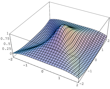
Figure 1: A 1+1 dimensional slice of the solution for two sources with the same charge is smooth and shows a 2-sphere shrinking and expanding.

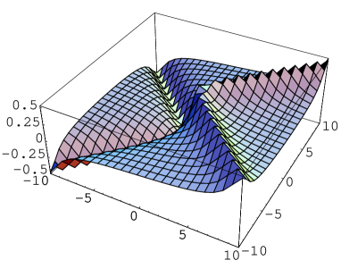
Figure 2: For two opposite charges, wave flips over in time which runs left to right.

Let us study the sources in this Wick rotation procedure. When we complexify the solution as (1.11), the locations of the sources are in fact also extended in the complex plane. For our present example with $C_{1}=C_{2}=C/2$ and $s_{1}=-s_{2}=s$, the location of the singularities are simply obtained by examining where the denominator of the complex solution vanishes,

$$(ix_{0}\pm s)^{2}+x_{1}^{2}+x_{2}^{2}+x_{3}^{2}=0.$$ (1.18)

The location of the singularities in this KG system are at

$$x_{0}=\sqrt{x_{1}^{2}+x_{2}^{2}+x_{3}^{2}}\pm is$$ (1.19)

Here we make a distinction between singularities and sources. The sources are point-like and at $x_{0}=\pm is$, they are distributed in imaginary space in terms of the $(x_{0},x_{1},x_{2},x_{3})$ coordinates. These sources generate the rest of the light-cone type singularities. Since the singularities are all at complex coordinates values, we can thus describe this as saying there are no real sources in the Klein-Gordon system. This is the reason why we obtained a source-free time-dependent solution of the Klein-Gordon system.

Having only dealt with the real part of the complexified solution, clearly there is also another solution which we can generate from the analytic continuation procedure, which is to take the case of two opposite charges with $C_{1}=-C_{2}=C/2i$ for real $C$

$$\phi = \frac{C/2i}{x_{1}^{2}+x_{2}^{2}+x_{3}^{2}+(ix_{0}-s)^{2}}-\frac{C/2i}{x_{1}^{2}+x_{2}^{2}+x_{3}^{2}+(ix_{0}+s)^{2}}$$ (1.20)

$$= \frac{Csx_{0}}{(-x_{0}^{2}+s^{2}+x_{1}^{2}+x_{2}^{2}+x_{3}^{2})^{2}+4s^{2}x_{0}^{2}}.$$

This solution is non-singular with the same “imaginary” singularity type structure as the previous case but just with different charges. A plot of the solution is shown in Fig. 2.

Note that the solution does not form a lump at the origin, is zero for $x_{0}=0$ and has a maximum and a minimum. This solution can be understood as the scalar field theory analogue of the gravity solutions generated from diholes of Ref. [5, 4]. Apparently the maximum and minimum values of the scalar field here correspond to the creation of large curvatures and therefore the horizons in the gravity solutions. The field theory solutions are different however in that they do not have an interpretation as the creation of a lower dimensional object as in the gravity case.

Of course it is possible that other solutions will generate divergences on the real $x_{0}$ axis even after analytic continuation. In such a case the Wick rotated system will also have a real source. For example, we can take the displacement of the sources in imaginary time to zero $s\rightarrow 0$, in which case these non-singular time dependent solutions to the wave equation do have a singular limit. These are the scalar field counterparts to the singular S-branes found in Ref. [7] where there is a spacelike source existing at one moment in time. We will further discuss the usefulness of imaginary sources in the following sections and define a new way to calculate their charges.

2 Imaginary Source Completeness

2.1 Our conjecture

We have seen that interesting time-dependent source-free solutions to the massless KG equation of motion can be obtained by applying the imaginary source technique. Then the following question naturally arises: what kind of solutions can we obtain from the technique? How general are the imaginary source solutions? Our answer to this question is the following conjecture:

Any regular solution to field equations in any theory has a corresponding distribution of sources in imaginary spacetime.

This statement is quite nontrivial. In this section, we provide a proof of this conjecture for wide variety of linear systems — massless/massive Klein-Gordon theories, and the Maxwell theory, in any dimensions. It will be shown that for every smooth solution of these theories, there is a corresponding imaginary source configuration. Surprisingly we will find that pairs of oppositely charged sources generate all the time dependent solutions in these cases, including the like charged source solutions. Hence dipole configurations play the crucial role as the basic ingredients of imaginary sources as opposed to single charges. With these insights we see that the status of imaginary sources is therefore promoted from curiosity to a powerful new viewpoint.

2.2 Proof for 1+0 dimensional Klein-Gordon system

A situation where the proof of the completeness conjecture can be explicitly and easily provided is the lowest dimensional example, that is, $1+0$ dimension. First let us consider the massless KG system.

The Euclidean solution with sources at $x=\pm s$ is easily written as

$$\phi=\left\{\begin{array}[]{ll}-iAx&(-s<x<s)\\ iAs&(x<-s)\\ -iAs&(s<x)\end{array}\right.$$ (2.24)

The magnitude of the source is given just by $\pm iA$. For simplicity we take the limit $s\to\infty$ to get just $\phi=-iAx$. The Wick rotation $x\to it$ gives

$$\phi=At$$ (2.25)

which is in fact a generic solution to the equation of motion in 1+0 dimensional KG system once a shift in real $t$ is included.

The same argument holds for massive case. We put sources at $x=\pm s$ in Euclidean space with opposite charges, and then take the $s\to\infty$ limit to get

$$\phi=Ae^{mx}+Be^{-mx}\ .$$ (2.26)

Then the Wick rotation gives

$$\phi=Ae^{imt}+Be^{-imt}$$ (2.27)

which is in fact a generic solution to the massive KG equation of motion.

After giving a proof for $1+1$ dimensions in the next subsection, in Sec. 2.4 we will prove the completeness of the massless/massive KG theories in any dimensions. Although the above proof in this subsection is straightforward, it will in fact also prove very useful. Before proceeding for that, here we present an issue of Wick rotation. Note that in the above we took $s\to\infty$ limit, but let us consider what happens if we didn’t take this limit. It seems that this limit is unnecessary because the change of $s$ does not modify the solution around the origin, $\phi=-iAx$. After the Wick rotation we look only at the imaginary axis of $x$. However, this sloppy argument contains a subtle issue which will be explained in Sec. 4.1.1. We have to take the $s\to\infty$ limit for completeness.

2.3 Proof for 1+1 dimensional massless Klein-Gordon system

For the massless KG system in 1+1 dimensions, the most general solutions to the equation of motion are known,

$$\phi=f(x-t)+g(x+t)$$ (2.28)

where $f$ and $g$ are arbitrary functions. We show that for any functions, $f$ and $g$, we have a corresponding distribution of sources in imaginary spacetime.

Our strategy in Sec. 1.2 for dealing with imaginary sources was to start with a Euclidean version of the field theory and to consider harmonic functions in that Euclideanized space. In two Euclidean dimensions spanned by $x$ and $y$, the harmonic function is $\phi=\log(x^{2}+y^{2})$ and so an array of such charges separated in the $y$-direction produces the field

$$\phi=\sum_{n}\frac{q_{n}}{4\pi}\ln(x^{2}+(y-y_{n})^{2}).$$ (2.29)

Here the source term should be given consistently by

$$\left(\partial_{x}^{2}+\partial_{y}^{2}\right)\phi=\sum_{n}q_{n}\delta(x)\delta(y-y_{n}).$$ (2.30)

Such a potential can also be interpreted as being generated by an infinitely long linear static source in 1+3 dimensions. Taking the analytic continuation $y\rightarrow-it$ of such a configuration we get

$$\phi=\sum_{n}\frac{q_{n}}{4\pi}\ln(-(t-iy_{n})^{2}+x^{2})\ ,$$ (2.31)

for which the source is given by

$$\sum_{n}q_{n}\delta(y)\delta(-it-y_{n}).$$ (2.32)

Evidently this means that the source is located at imaginary time.

For illustration, begin with the case of two sources separated by a distance $s$

$$\phi=\frac{q}{2\pi i}\left[\ln(x^{2}+(y-s/2)^{2})-\ln(x^{2}+(y+s/2)^{2})\right].$$ (2.33)

The normalization of the charge has been chosen for the later purpose. The Wick rotation gives a Lorentzian solution which is completely regular,

$$\phi=\frac{q}{2\pi i}\left[\ln(-(t-is/2)^{2}+x^{2})-\ln(-(t+is/2)^{2}+x^{2})\right]$$ (2.34)

which can be simplified to

$$\phi=\frac{q}{\pi}\arctan\frac{ts}{x^{2}-t^{2}+s^{2}/4}\ .$$ (2.35)

This solution, as shown in Fig. 4, is related to two opposite charged sources and is asymptotically flat. Now because the arctangent function is multi-valued, we have to specify the period of the values which the function takes. For the solution to be smooth also in derivatives we choose the branches of the arctangent to take

$$\left\{\begin{array}[]{ll}0<\phi/q\leq 1&(t>0)\\ -1\leq\phi/q<0&(t<0)\ .\end{array}\right.$$ (2.38)

Choosing branches in this fashion amounts to three different branches of arctangent which smoothly fit together. The solution is created to be spatially symmetric under $x\rightarrow-x$. However it is clearly also antisymmetric in time $t\rightarrow-t$ and therefore imaginary time so the solution must vanish at $t=0$.

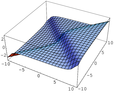
Figure 3: Imaginary part of log wave with two oppositely charged imaginary sources at $t=\pm i$ is asymptotically flat at infinity. It is an upside down wave coming in from past infinity and then it flips to an upright wave; time runs left to right in the figure.

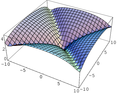
Figure 4: Real part of log wave with two same charged imaginary sources at $t=\pm i$; time runs left to right in the figure.

We could also take the two like charged solutions instead, whose Wick rotation would give, up to a proportional constant,

$$\phi=\ln(\sqrt{(x^{2}-t^{2}+s^{2}/4)^{2}+t^{2}s^{2}})\ .$$ (2.39)

Although this solution will not turn out to play an important role in the following discussion, this solution is plotted in Fig. 4 and is new in that the potential is not flat at infinity.

Let us look at the asymptotic region of the solution (2.35) in more detail. We can take a limit $x+t\to\infty$ while keeping $x-t$ finite and fixed, which gives

$$\phi\to\frac{q}{\pi}\arctan\frac{s/2}{x-t}.$$ (2.40)

This shows that the asymptotic region is in fact a wave packet whose width is given by $s$ and whose amplitude is not decaying but a constant. In other words, the asymptotic solution is in fact a (localized) plane wave. Because this plane wave has an arbitrary real parameter $s$ which is the width, we can generically expect that this S-brane solution may form a basis for a function space in 1+1 dimensions, as the plane waves do. Below we present a precise proof of the completeness.

As suggested in the generic form of the solution (2.28), one can show that the solution (2.35) is written as a collision of two wave packets,

$$\phi=\frac{q}{\pi}\left(\arctan\frac{-s/2}{x+t}-\arctan\frac{-s/2}{x-t}\right)$$ (2.41)

not asymptotically but exactly. Here the arctan functions are chosen to take values in $0<\arctan<\pi$. Let us take the thin wall limit $s\to 0$, then the solution becomes

$$\phi=q\left(\theta(x+t)-\theta(x-t)\right).$$ (2.42)

The corresponding sources are distributed at $(t,x)=(\pm s,0)$, or more precisely, the source is given by the distribution function

$$\lim_{s\to 0}\frac{2q}{i}\delta(x)\left[\delta(-it-s/2)-\delta(-it+s/2)\right].$$ (2.43)

The solution in this limit(2.42) seems to serve as a basis of the generic solution (2.28), but unfortunately it leaves a constraint between the amplitudes of the left and right moving modes. This difficulty can not be overcome by adding combinations of the same sources displaced relative to each other since each source suffers from the same left-right mode symmetry. To overcome this difficulty, we must introduce a new solution whose imaginary source is located at $(t,x)=(0,\pm is)$, that is, the solution obtained by exchange of the roles of $t$ and $x$. What we get as a result of the sum of those four sources is the solution (see Fig. 5)

$$\phi=q(2\theta(x+t)-1).$$ (2.44)

This is a purely left-going wave of a step function. Interestingly, this procedure to get a purely left-mover introduces the new idea of sources at imaginary space.

Figure 5: Addition of the original solution with imaginary time source and the new solution with imaginary space source gives a purely left-moving wave.

At this stage it is quite easy to see that this forms a basis for generating all the solutions (2.28), because a derivative of this step function is in fact a delta function $\delta(x+t)$. Thus, adding various imaginary source distributed as the following source term

$$\lim_{s\to 0}\int\!dx_{0}dt_{0}\;\left[\frac{2q(x_{0},t_{0})}{i}\delta(x-x_{0})\biggl{(}\delta(-i(t-t_{0})-s/2)-\delta(-i(t-t_{0})+s/2)\biggr{)}\right.$$

$$\hskip 56.9055pt\left.+\frac{2\tilde{q}(x_{0},t_{0})}{i}\delta(t-t_{0})\biggl{(}\delta(-i(x-x_{0})-s/2)-\delta(-i(x-x_{0})+s/2)\biggr{)}\right]\hskip 28.45274pt$$ (2.45)

we may reproduce the generic solution (2.28). Here the second term is given by the exchange of the roles of $t$ and $x$, and we let the source amplitude $q$ and $\tilde{q}$ to be dependent also on the real spacetime $(x_{0},t_{0})$. In fact, if we choose

$$q(x_{0},t_{0})=-f^{\prime}(x_{0}-t_{0})\delta(x_{0}+t_{0})+g^{\prime}(x_{0}+t_{0})\delta(x_{0}-t_{0}),$$ (2.46)

$$\tilde{q}(x_{0},t_{0})=f^{\prime}(x_{0}-t_{0})\delta(x_{0}+t_{0})+g^{\prime}(x_{0}+t_{0})\delta(x_{0}-t_{0}),$$ (2.47)

a straightforward calculation reproduces (2.28). This is a proof of the imaginary source completeness in the 1+1 dimensional massless Klein-Gordon system. We see in this non-trivial example the power and relevance of imaginary sources as being a possible way to understand all features of time dependence.

2.4 Proof in any dimensions for Klein-Gordon and Maxwell systems

Using the results of the previous subsections, we give a simple argument to show the completeness of imaginary sources in any dimensions of the Klein-Gordon system and the Maxwell system.

Massive Klein-Gordon

First, let us consider the massive Klein-Gordon system. Any configuration of the field $\phi$ has a representation in terms of Fourier basis,

$$\phi(x)=\int d^{d+1}k\;F(k)e^{ik_{\mu}x^{\mu}}.$$ (2.48)

For this configuration to be a solution of the equation of motion, we know that the plane wave is necessarily on-shell,

$$k_{0}^{2}-k_{i}^{2}-m^{2}=0\quad(i=1,2,\cdots,d).$$ (2.49)

Therefore once this Fourier basis is constructed in terms of the imaginary source in time, a proof of the completeness is given. In fact it is very easy to obtain the corresponding imaginary source distribution, if one performs a Lorentz transformation on the above momentum to get

$$k_{0}=\pm m,\quad k_{i}=0.$$ (2.50)

This plane wave is just the same as what we obtained in the 1+0 dimensional case of subsection 2.2. So if we distribute the imaginary source of the previous subsection to also fill all the real spatial dimensions, and perform the Lorentz transformation back, then we certainly get the plane wave with the momentum (2.49). Completeness of the imaginary sources is therefore proven in massive Klein-Gordon theory.

Note that it is not necessary to introduce imaginary space sources in the massive Klein-Gordon case to remove the left/right moving symmetry as was needed in the case of massless Klein-Gordon. This is due to the fact that one can reduce the entire problem of the massive Klein-Gordon case to 0+1 dimensions which does not have left/right moving modes.

Massless Klein-Gordon

For massless KG theory, we may employ a similar argument. In this case the on-shell condition for the momentum of the plane wave is

$$k_{0}^{2}-k_{i}^{2}=0\quad(i=1,2,\cdots,d),$$ (2.51)

and a proper Lorentz transformation leads to

$$k_{0}=\pm k_{1},\quad k_{2}=k_{3}=\cdots=k_{d}=0.$$ (2.52)

Having reduced the situation to the case of 1+1 dimensions, we can apply our completeness proof from Sec. 2.3. There we wrote down explicitly the distribution of imaginary sources needed to reproduce a plane wave with momentum (2.52). Applying the inverse Lorentz transformation gives us the desired source distribution in arbitrary $1+d$ dimensions thereby explicitly proving the completeness conjecture.

Maxwell system

Interesting solutions of the Maxwell system will be given in Sec. 4.3, but here we shall give a proof of the completeness for this system. The proof follows once we have the proof for the massless Klein-Gordon system: in a Lorentz gauge all the equations of motion in the Maxwell system are identical to that of the massless Klein-Gordon system. This is enough to know that all the Maxwell regular solutions can have imaginary source interpretation. One difference however is that the charge for Klein-Gordon is a scalar while the charge for Maxwell theory is a vector/one form. Lorentz transformations will therefore act differently on these charges as opposed to the scalar Klein-Gordon charges.

3 Capturing Moving Charges

In this section we discuss a new definition of S-brane charge which we apply to our imaginary source solutions and find that it characterizes the imaginary source solutions. We show that in the correct limit it reduces to the usual charge definition of a static charge. This new definition of S-charge is also compared with previous definitions [7, 4, 5].

3.1 A new definition of S-charge

In the case of Euclidean spacetimes, we surround a point by choosing another distinct point and then applying the rotation group preserving the distance from the source. This generates a sphere surrounding the source. One can take the limit where we are far from the source at spatial infinity and place flux detectors there to count the charge. This is illustrated in a Penrose diagram in Fig. 7.

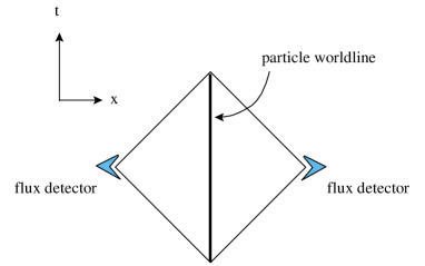
Figure 6: In Minkowski space, we can measure the charge of a stationary particle by surrounding it with flux detectors at spatial infinity. This is labeled in the Penrose diagram.

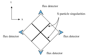
Figure 7: To calculate the charge of a spacelike source, we measure the flux by going to timelike and spatial infinity. The lightcone singularities generate a source at their intersection point.

In the case of Lorentzian spacetimes and spacelike sources, the rotation group is disconnected. We wish to cover the source with hyperboloids. In fact this is a generalization of the notion of surrounding a charge in Lorentzian signature spacetimes. Each connected piece of the Lorentz group will generate one of three hyperboloids.

In 3 dimensions, we have three hyperboloids: $x^{2}+y^{2}-\tau^{2}=a^{2}$, which we call $H_{2}$, is a connected hyperboloid; and $x^{2}+y^{2}-\tau^{2}=-a^{2}$ gives two disconnected hyperboloids which we call $H_{1},H_{3}$ as shown in Fig. 8.

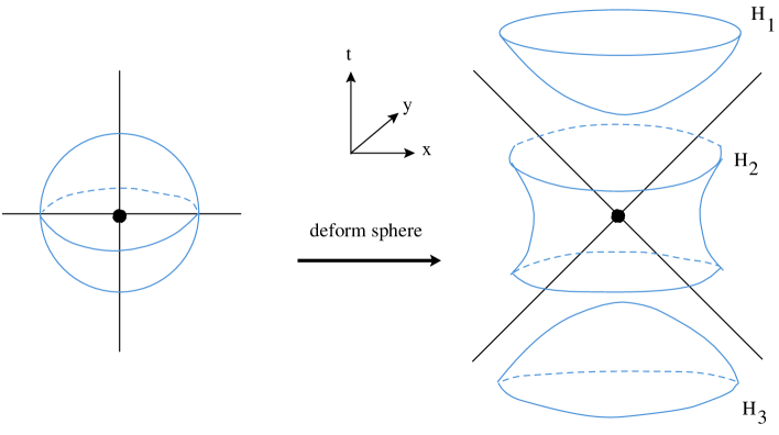
Figure 8: To surround a spacelike source we must capture flux in the time and spacelike directions.

If we take the limit of these hyperboloids to infinity, we see that we should place flux detectors at spatial and timelike infinity as shown in the Penrose diagram of Fig. 7 to completely enclose the source. Such a notion of surrounding a spacelike charge makes sense in spacetime as opposed to space.

One possible problem with these choices for hyperboloids however is that the area of this hyperboloid is infinite. While for a sphere a fixed radius area is $\int_{S^{2}}r^{2}\sin\theta d\theta d\phi=4\pi r^{2}$, we have for a hyperboloid $\int_{H^{2}}r^{2}\cosh\theta d\theta d\phi=\infty$ for $r\neq 0$. One point to note then before doing the calculation is that the induced metric on the connected hyperboloid is positive while the induced metric on the two disconnect hyperboloids is negative. For the connected hyperboloid, $H_{2}$, we have $x=a\cosh\theta\cos\phi$, $y=a\cosh\theta\sin\phi$, $t=a\sinh\theta$. For the disconnected hyperboloids $H_{1},H_{3}$ we have $x=a\sinh\theta\cos\phi$, $y=a\sinh\theta\sin\phi$, $t=\pm a\cosh\theta$ and we also notice that to cover the hyperboloids once we only need $\theta\in[0,\infty)$. Calculating the area integral we have for one disconnected hyperboloid and half of the connected hyperboloid $-\int_{0}^{\infty}a^{2}\sinh\theta d\theta d\phi+\int_{0}^{\infty}a^{2}\cosh\theta d\theta d\phi=2\pi a^{2}$. Note the minus sign intuitively comes from the fact that one are is timelike and one spacelike. If we include the contribution from the other half we get that the total area of the three hyperboloids is $4\pi a^{2}$! This is exactly then an analytic continuation of a sphere’s area.

Now let us consider a source, a delta function. For the case of Euclidean 3 dimensional space we have that integrating the flux generated by a delta function over a 2-sphere is $\int_{S^{2}}\frac{\hat{r}}{r^{2}}\cdot\hat{r}r^{2}\sin\theta d\theta d\phi=4\pi$. For the Wick rotated case we have upon integrating the Green’s function over the three hyperboloids

$$\left(\int_{H^{2}_{1}}+\int_{H^{2}_{2}}+\int_{H^{2}_{3}}\right)\frac{\hat{\eta}}{\eta^{2}}\cdot\hat{\eta}\eta^{2}(\cosh\theta-\sinh\theta)d\theta d\phi=4\pi\ ,$$ (3.53)

where $\eta^{2}\equiv-t^{2}+x^{2}+y^{2}$. This verifies the consistency of the definition of the delta function for spacelike sources with the new definition of S-charge.

3.2 Charge of the nonsingular time-dependent solutions

Let us next try to apply this new rule of charge counting for our non-singular imaginary sources. The explicit calculation is simplified by calculating at large values from the light cone. Remember for two static charges at $x=\pm s$ that the potential is

$$\phi=\frac{1}{\sqrt{(x-s)^{2}+y^{2}+z^{2}}}+\frac{1}{\sqrt{(x+s)^{2}+y^{2}+z^{2}}}\ .$$ (3.54)

Although the configuration is non-spherical, the charge of this system is easy to calculate for large values of $r^{2}=x^{2}+y^{2}+z^{2}$ where the solution simplifies to

$$\phi=\frac{2}{\sqrt{x^{2}+y^{2}+z^{2}}}+{\cal{O}}\left(\frac{1}{r^{2}}\right)$$ (3.55)

using a simple Taylor expansion. To calculate the charge at infinite radius, we see that the higher order terms do not contribute and so the charge simply is $Q=2$.

We now try to similarly calculate the charge in the case time dependent solutions with imaginary sources. For example the Wick rotation of the above case gives

$$\phi = \frac{1}{\sqrt{(it-s)^{2}+y^{2}+z^{2}}}+\frac{1}{\sqrt{(it+s)^{2}+y^{2}+z^{2}}}$$ (3.56)

$$= \frac{\sqrt{2}}{((\eta^{2}+s^{2})^{2}+4t^{2}s^{2})^{1/4}}\sqrt{1+\frac{\eta^{2}+s^{2}}{\sqrt{(\eta^{2}+s^{2})^{2}+4t^{2}s^{2}}}}.$$

where $\eta^{2}\equiv|-t^{2}+y^{2}+z^{2}|$. For large $\eta\gg s$, we have an expansion

$$\phi = \frac{2}{\eta}+{\cal{O}}\left(\frac{1}{\eta^{2}}\right)\ .$$ (3.57)

We see that this has a S-charge $Q=2$. Despite the fact that there are neither real sources nor singularities, this non-singular solution has a charge! In this case the charge is the same regardless of how close we are to the lightcone since there are no real sources. On the other hand if the imaginary sources have opposite charges, their S-charge is zero. This is clear from Fig. 2 where we see a wave coming in and flipping over. The contributions from the past and future light cone regions clearly cancel to give zero S-charge.

3.3 Lorentzian Gauss law

It should be emphasized that in the case of the nonsingular solutions, our notion of charge seems to be conserved only in an asymptotic sense. Let us explain more concretely the deformations of the integration surfaces.

In the usual definition of charges in Euclidean space, we are allowed to deform the integration surface arbitrarily to enclose sources. This is due to the Gauss’s theorem. A simple statement about Gauss’s theorem in $1+2$ Lorentzian spacetime is as follows. Surround the origin with a cube with sides at $\frac{1}{2}(\pm\Delta x_{0},\pm\Delta x_{1},\pm\Delta x_{2})$. For a scalar field $\phi$, the flux through the spatial direction $x_{2}$ is

$$\nabla\phi\left(\frac{\Delta x_{2}}{2}\right)\cdot\hat{x}_{2}\ \Delta x_{1}\Delta x_{0}+\nabla\phi\left(-\frac{\Delta x_{2}}{2}\right)\cdot\left(-\hat{x}_{2}\right)\ \Delta x_{1}\Delta x_{0}$$ (3.58)

which under Taylor expansion is

$$\partial_{x_{2}}^{2}\phi(0)\ \Delta x_{0}\Delta x_{1}\Delta x_{2}\ .$$ (3.59)

The only difference for the flux calculation along the timelike direction is that the unit vector has negative norm $\hat{x}_{0}\cdot\hat{x}_{0}=-1$ so the flux in the $x_{0}$ timelike direction is

$$-\partial_{x_{0}}^{2}\phi(0)\ \Delta x_{0}\Delta x_{1}\Delta x_{2}\ .$$ (3.60)

In total the flux through the square is

$$(-\partial_{x_{0}}^{2}+\partial_{x_{1}}^{2}+\partial_{x_{2}}^{2})\phi(0)\ \Delta x_{0}\Delta x_{1}\Delta x_{2}$$ (3.61)

so the generalized Gauss law in Lorentzian spacetimes ($\mu=0,1,2$) is simply

$$\int\partial_{\mu}\partial^{\mu}\phi\ d^{3}x=\int\nabla\phi\cdot\hat{n}\ d^{2}S\ .$$ (3.62)

Instead of just restricting ourselves to using box-like integration regions, let us further expand on the notion of surrounding spacelike sources. A sphere surrounds a point particle in Euclidean space, and a sphere in spacetime also surrounds a spacelike source. Arbitrary deformation of the bounding surface are allowed as long as we do not pass through additional charges. One can imagine then a large deformation of the bounding surface where the edge stretches far from the source. If the limit in which the contour deformation is taken to infinity carefully, then the charge bounded must remain constant.

For example in the case of the singular solution, there is a concrete source producing an associated charge. For the non-singular sources there is always an associated charge as calculated using our prescription. However if deformations of the hyperboloids to a sphere are smooth, then we take the resulting sphere to zero radius and the charge accordingly vanishes due to the smoothness of our solutions. Therefore we should understand that our prescription of using hyperbolas for the S-charge is not necessarily topologically equivalent to the sphere which can shrink. The integration surfaces consist of three hyperboloids in the case of 1+2 dimensions, and they are disconnected, that is why we obtained nonzero S-charge for non-singular field configurations.

3.4 Comparison with previous charge definitions

Let us discuss relations to the previous definitions of spacelike charges. A definition of spacelike charge for the case of 1+1 dimensional Klein-Gordon was presented as an example in Ref. [7]. As discussed there one choice of propagator is $\phi(u=t+x,v=t-x)=\theta(u)\theta(v)$ as it satisfies

$$\partial_{u}\partial_{v}\phi(u,v)=\delta^{2}(u,v)\ .$$ (3.63)

This solution satisfies a straightforward but probably unfamiliar Gauss law equation which is still of the form $\int_{V}d*d\phi=\int_{\partial V}*d\phi$ but where the integral is now over the space and time direction. First let us calculate the S-charge of this configuration using the definitions of Ref. [7] where we enclose the spacetime origin. If we integrate over a rectangle in lightcone coordinates with corners at $(u,v)=(\pm a,\pm b)$, we calculate the charge of this solution to be

$$Q=\int\!\!*d\phi=\oint\!\left[\delta(u)\theta(v)du-\delta(v)\theta(u)dv\right]=\int_{-a}^{a}\!\!\!\!\!\theta(b)\delta(u)du-\int_{b}^{-b}\!\!\!\!\!\!\!\theta(a)\delta(v)dv=2\ .$$

If we take this configuration to be a solution to Maxwell theory in 1+2 dimensions, we must also impose the current conservation law $\partial_{t}\rho+\partial_{x}J_{x}=0$ which introduces the spacelike current $J_{x}=-\theta(x)\delta^{\prime}(t)$.

Let us compare this result with our prescription for the S-charge. In this 1+1 dimensional case, four disconnected hyperbolas are needed to bound the source. The propagator $\Phi=\theta(u)\theta(v)$ can be written in terms of Milne $(t,x)=\pm(T\cosh r,T\sinh r)$ and Rindler coordinates $(t,x)=\pm(-T\sinh r,T\cosh r)$. In the Milne region $t>|x|$ we calculate the charge to be

$$\int_{M}*d\Phi=\int[-\delta(Te^{r})\theta(Te^{-r})e^{r}T-\delta(Te^{-r})\theta(Te^{r})e^{-r}T]dr$$

$$\hskip 56.9055pt+[-\delta(Te^{r})\theta(Te^{-r})e^{r}+\delta(Te^{-r})\theta(Te^{r})e^{-r}]dT\ .$$ (3.64)

For simplicity take the integral to be at fixed $T$ and from $r=(-\infty,\infty)$ and change variables to obtain

$$\int_{M}*d\Phi=\int_{0}^{\infty}-\delta(w)\theta(T/w)dw-\delta(w)\theta(T/w)dw=\frac{1}{2}\theta(T\cdot\infty)+\frac{1}{2}\theta(T\cdot\infty)=1$$ (3.65)

where we have used the identity

$$\int_{0}^{\infty}\delta(x)dx=1/2.$$ (3.66)

Although the delta function is sharply defined at $x=0$, we define by the meaning of our hyperbolic integral this symmetric condition on the integration of the delta function. In the second Milne region $t<-|x|$ we find that the answer is zero $Q=0$. This can be seen simply since we can obtain this second region from the first by simply replacing $T\rightarrow-T$. The final charge will then depend on $\theta(-T\infty)=0$ giving zero charge.

For the Rindler region $x>|t|$ we find the charge integral becomes

$$\int_{R}*d\Phi=\int[\delta(Te^{-r})\theta(-Te^{r})e^{-r}T-\delta(-Te^{r})\theta(Te^{-r})e^{r}T]dr$$

$$\hskip 56.9055pt-[\delta(Te^{-r})\theta(-Te^{r})e^{-r}+\delta(-Te^{r})\theta(Te^{-r})e^{r}]dT\ .$$ (3.67)

Again integrating at fixed $T$ from $r=(\infty,-\infty)$ and using our above definition of integrating delta functions

$$\int_{R}*d\Phi=\int_{0}^{\infty}\delta(w)\theta(-T/w)dw-\delta(w)\theta(T/w)dw=\frac{1}{2}\theta(T\cdot\infty)=\frac{1}{2}$$ (3.68)

we get a charge contribution of $1/2$. Similarly in the second Rindler region the answer is $1/2$. In total, the charge of this spacelike source is $Q=2$ just like when we integrated before. In this case we have defined the hyperbolas to bound the charge which results in the same charge.

Note that the charge using the hyperbolas would take a different value if we used a different way of evaluating the boundary of the integrals. Here we took only half of the delta function as in (3.66), but if we define the integral as $\lim_{\epsilon\to 0}\int_{\epsilon}^{\infty}dw$ then the resulting S-charge is zero. With this definition of the boundary with $\epsilon$, the hyperbolas of the integral never touch the lightcones and so with this definition it does not enclose the origin where the source resides.

Before ending this subsection, we evaluate the charge of the Wick rotated logarithm harmonic function in two dimensions using the definition of Ref. [7]. The solution to the Green’s function in 2 dimensional Euclidean space is known to be $(1/4\pi)\ln(x^{2}+y^{2})$ and its Wick rotation $(1/4\pi)\ln(x^{2}-t^{2})$ was the basis of our discussion in the previous section. Although we have referred to this kind of solution as a delta function for the wave equation due to analytic continuation, this kind of procedure is a bit subtle in the presence of delta functions. Let us therefore verify the form of singularity by applying Gauss’s theorem as before. To ensure that Wick rotation is consistently working we check the charge of this Wick rotation using once again light cone coordinates $(u,v)$. Taking into account the $i\epsilon$ prescription which rewrites integrals in terms of the principal value and delta functions we have

$$*d\ \ln(x^{2}-t^{2})=\frac{vdu-udv}{uv+i\epsilon}$$ (3.69)

$$Q=\int\left[vdu\left(P\left(\frac{1}{uv}\right)-i\pi\delta(uv)\right)-udv\left(P\left(\frac{1}{uv}\right)-i\pi\delta(uv)\right)\right]$$

$$\hskip 14.22636pt=\int\left[-i\pi\ {\rm Sign}(v)\delta(u)du+i\pi\ {\rm Sign}(u)\delta(v)dv\right]=4\pi i$$ (3.70)

so the solution $\phi=(i/4\pi)ln(x^{2}-t^{2})$ has a unit of S-charge.

3.5 Relation to usual static charge

In this subsection we count more complicated configurations of charge. First take the case of two S-branes shifted in time as discussed further in Sec. 4.1.2. Our rule is to surround both S-branes by a single large hyperboloid as shown in Fig. 9.

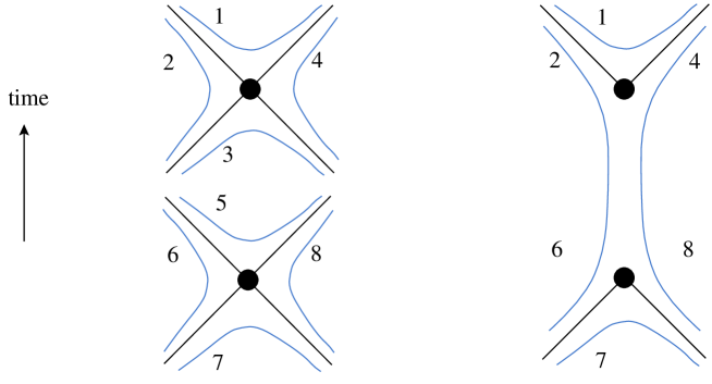
Figure 9: Surround two spacelike source using hyperbolas, and then cancel contributions whenever possible. For example contributions from hyperbolas 3 and 5 cancel. After making all possible cancellations we are left with a similar configuration as for one S-brane.

These hyperbolas have cancelling contributions and we can deform the calculation into three hyperboloids again as shown in Figure 9. The calculation for two S-charges is similar to that of one S-charge. In the process we must integrate over the lightcone discontinuities.

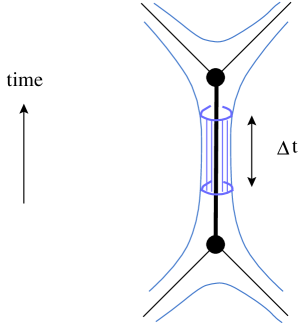
Figure 10: The integral over a small region of a hyperbola turns into an integral over a cylinder with the circle in the space directions and the length of the cylinder along time.

A further interesting observation which shows the consistency of our definitions is the following. Allow for a linear distribution of singular spacelike sources in the time direction as we will discuss in Sec. 4.1.2. Generalizing the definition of S-charge just outlined above for two charges then we should integrate over three disconnected regions. If the S-brane is long lived then two of the regions are past the singularities and do not contribute much to the total S-charge. We are just left with then a circular integral of the usual charge for a particle, times an integral over time as shown in Fig. 10

$$Q_{\textup{S-charge}}=Q_{\textup{static charge}}\cdot\Delta t\ .$$ (3.71)

Our definition of S-charge is then related to the usual charge of a static particle charge in the same way as static charge is related to a linear charge density in space, $Q=\lambda L$. In this way our definition of S-charge reproduces the usual static charge. Our S-charge is therefore also consistent with the fact that integrating singular spacelike sources over time reproduces the potential of an static charged particle as we will mention in Sec. 4.1.2. Because spacelike sources can be thought of concretely as the individual bits of a particle’s worldline trajectory, there is something quite fundamental about spacelike sources in time dependent systems as opposed to particles.

3.6 Secondary S-charge

In addition to the above definition of S-charge, there has also been a definition of S-brane charge proposed in Ref. [4]. First let us review this definition. Turning away from the Klein-Gordon equations, consider the a positive charge and a negative charge forming a dipole. There are three charges we can calculate which are the dipole charge and also each individual charge. Place a negative/positive charge at $z=\pm s$ so the potential is $\phi=\frac{c}{\sqrt{x^{2}+y^{2}+(z-s)^{2}}}-\frac{c}{\sqrt{x^{2}+y^{2}+(z+s)^{2}}}$. We surround the negative charge by a two sphere which we deform until it fills out the half plane between the two charges and goes out to infinity in the upper half plane. The electric field along this $z=0$ plane is

$$E_{z}=\frac{-c(z-s)}{(x^{2}+y^{2}+(z-s)^{2})^{3/2}}+\frac{c(z+s)}{(x^{2}+y^{2}+(z+s)^{2})^{3/2}}=\frac{2cs}{(x^{2}+y^{2}+s^{2})^{3/2}}.$$ (3.72)

If we change variables so $\rho^{2}=x^{2}+y^{2}$ then the flux through the half plane is

$$\Phi=\int E_{z}\rho d\rho d\phi=2\pi\int\frac{2cs}{(\rho^{2}+s^{2})^{3/2}}\rho d\rho=2\pi(2cs)\frac{1}{\sqrt{\rho^{2}+s^{2}}}\biggm{|}^{\infty}_{0}=-4\pi c$$ (3.73)

which is the same as the calculation using the usual sphere. Such a charge definition works only on two opposite charges and is zero when the charges are the same. This method picks up one of the charges but only in a dipole configuration. The flux calculation is of course the same for any choice of infinite half plane between the two charges; the only difference is that there will be also be contributions from the electric field in the other $(x,y)$ spatial directions.

Wick rotating the two oppositely charged sources by $z\rightarrow i\tau$ does not affect the above charge calculation. What we have though is a different interpretation of the charge. The potential $\phi=A_{0}\rightarrow A_{4}$ and the original electric field along the $z$ direction becomes an electric field along the $x^{4}=i\tau$ direction so overall $F_{tz}=F_{x^{4}\tau}$. Specifically the electric field along $x^{4}$ at time $\tau=0$ is

$$E_{x^{4}}=\frac{2cs}{(x^{2}+y^{2}+s^{2})^{3/2}}$$ (3.74)

and the rest of the calculation is the same. Calculating the flux at a different time gives the same answer but the difference is that now there is also the presence of time dependent magnetic fields. If we were to calculate the charge of such a potential in a scalar field theory, we would obtain zero S-charge according to our prescription since this is a wave which flips its amplitude.

Summarizing the difference between the definitions of S-charges, we find that our new definition of S-charge seems consistent with the notion of calculating the flux from putting in a single delta function sources in time. It is also able to calculate the total amount of charge which is focused into a small region of space and time. The notion of S-brane charge in Ref. [4] on the other hand is a way to calculate the charge of dipole type configurations. These two charge definitions produce different results in the cases we have studied. However it is very natural for spacelike sources to have various charges. We are well familiar with the fact that distributions of electric charges have monopole, dipole, quadropole, and higher multipole moments and that is something similar to the situation here.

4 Explicit Examples

In this section we provide explicit examples of the imaginary source solutions for massless/massive Klein-Gordon systems and also for Maxwell system. In particular, Wick rotations of electrons, monopoles and instantons are shown to give cylindrical/spherical electromagnetic waves.

4.1 Arrays of massless Klein-Gordon solutions

4.1.1 Infinite imaginary arrays

Arrays in 4 dimensions

In Euclidean space, let us take an infinite array of alternating point charges. The potential is

$$\phi_{\rm array}=\sum_{n=-\infty}^{\infty}\frac{C_{1}}{(x_{4}-s/2+2ns)^{2}+r^{2}}+\frac{C_{2}}{(x_{4}+s/2+2ns)^{2}+r^{2}}$$ (4.75)

where $r^{2}\equiv(x_{1})^{2}+(x_{2})^{2}+(x_{3})^{2}$. We have been dealing with finite numbered arrays but what about infinite numbered arrays like the one above? Does it even give a well defined potential when we are away from the point charges? Although an infinite array may seem like a very special configuration, it is important to discuss this case especially in relationship to the rolling tachyon.

Let us check that $\phi_{array}$ is bounded when away from a single charge, for the case of real $C_{1}=C_{2}$. First it clear that the denominators are squares of positive numbers and so will be minimized when each positive number is as small as possible. This means that we should take $r=0$. Due to the periodicity of the solution we know that we can maximize the solution by simply maximizing it in the range $-s/2<x_{4}<s/2$. In this range all terms with $n\neq 0$ are maximized at $x_{4}=\pm s/2$. Summing all such non-singular terms the sum is bounded by

$$\phi_{\rm array}<\sum_{n=-\infty}^{\infty}\frac{2}{(2ns)^{2}}+\frac{1}{(x_{4}-s/2)^{2}}+\frac{1}{(x_{4}+s/2)^{2}}\ .$$ (4.76)

The infinite sum is bounded and the remaining two terms are only divergent at the singularity. By taking absolute values, we can likewise show that arrays of positive and negative charges ($C_{1}=-C_{2}$) give a bounded sum for the potential except for when we are at a source.

In the case of time dependent solutions, we can similarly bound the potential. One easy way to check this statement is to realize that the potential for two positive charges was seen to maximized at the origin of spacetime (see Fig. 2). This means that for each pair of same charges in the infinite sum the same is true that the potential is maximized at $x_{0}=0,x_{1}=x_{2}=x_{3}=0$. This again reduces the sum to an infinite series of inverse squares which is finite. The difference is that in this case, all the terms are non-singular since we can never approach any of the singularities at $x_{0}=\{\rm imaginary\ values\}$. We conclude that the potential is completely bounded. As pointed out in Ref. [2], this infinite summation can be done explicitly for $C_{1}=C_{2}=C$, using the relationship

$$\tanh z=\lim_{n\to\infty}\sum_{k=-n}^{n}\frac{1}{i\pi(\frac{1}{2}-k)+z}\qquad\mbox{for }\quad\frac{iz}{\pi}-\frac{1}{2}\notin{\bf Z}$$ (4.77)

we find the non-singular form

$$\phi_{\rm RT} = \sum_{n=-\infty}^{\infty}\frac{C}{-(x_{0}-is/2+2ins)^{2}+r^{2}}+\frac{C}{-(x_{0}+is/2+2ins)^{2}+r^{2}}$$ (4.78)

$$= \frac{1}{r}\frac{C\pi}{2s}\left[\tanh\left(\frac{\pi}{s}(-x_{0}+r)\right)+\tanh\left(\frac{\pi}{s}(x_{0}+r)\right)\right]$$

At time $x_{0}=0$ this function is monotonically decreasing as a function of the radius $r$ from the value 1 to zero. This can be interpreted as a localized lump. For large values of the radius $r\gg(x_{0},s)$, we have that this is a nearly static potential. Furthermore, this has a characteristic behavior $\phi_{\rm RT}\sim 1/r$ as opposed to the original $1/r^{2}$ contribution from each source. In the far past and far future, this potential goes to zero.

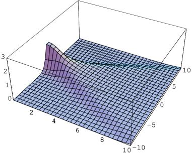
Figure 11: An infinite array of like codimension four charges is asymptotically in the spacelike direction a codimension three particle and a decaying wave in the past and future. The lightcone clearly separates the characteristics in the two different regions.

Here we see that arrays of imaginary sources of codimension four, can create time dependent versions of real sources of codimension three. In effect we are creating a nonsingular time dependent version of a static point source! This can be understood from the fact that an infinite summation of sources is effectively an integral and so the $1/r^{2}$ behavior sums to $1/r$. Imaginary source summation is not effectively a summation over time but a summation over space because of the “$i$” imaginary factor. Therefore essentially any infinitely extended in imaginary space summation of one type of charge will lead to the same kind of asymptotic $1/r$ behavior at spatial infinity.

A peculiar fact about such infinitely extended solutions is that at fixed time and large radius, these solutions have finite static charge. By “static charge” here we mean integrating the three form $*d\phi$ over the time direction and angular directions at a fixed radius, $\int_{\Delta t,\Omega}*d\phi$. Next divide the integral by the period of time we integrate over and this averaged result is what we mean by the static charge. If we take the limit of the radius to infinity first, then the static charge is a finite constant. Therefore an observer would expect to see an electron at the origin. However over a long enough period the time dependent terms have a dramatic effect and are not ignorable in general. The effect of time dependence is to transport the field configuration to and from infinity.

While we discussed infinite arrays of one type of charge, we can also discuss what happens to alternating charge arrays. In fact only these dihole charge type solutions have known gravity solution duals [4, 5]. It is actually a simple process to produce the infinite array of such solutions, since the sum of alternating charges can equivalently be thought of as the sum of two infinite arrays of like charges. Simply take the above solution and translate $x_{0}\to x_{0}+is/4$ and take the imaginary part of the result. Using the standard hyperbolic tangent addition rule we get[2]

$$\phi_{\rm RT2}=\frac{1}{r}\frac{C\pi}{s}\left[\frac{1}{\cosh(2\pi(r+x_{0})/s)}-\frac{1}{\cosh(2\pi(r-x_{0})/s)}\right]$$ (4.79)

which is clearly going to zero at large radial values and in the far past and future.

One can also modify the charges $C_{1}$ and $C_{2}$ so that they are dependent on $n$. As long as the modification is mild (the charge does not grow as $n$), the final sum is convergent and well-defined. This variation corresponds to various fine structure of the spherical shell shrinking and expanding.

Arrays in 1 dimension

Each source localized in one dimension generates a linear potential, $\phi=|x-a|$, which has a derivative discontinuity. Although taking an array of such sources is a bit subtle due to the infinities involved, a consistent representation is the triangle wave function. Placing negatively charged sources at $x=s/2+2ns$ and positively charged sources at $x=-s/2+2ns$ for all integers $n$, then the potential is $\phi=2x/s$ for $x=[0,s/2]$, $\phi=2-2x/s$ for $x=[s/2,3s/2]$ and $\phi=-4+2x/s$ for $x=[3s/2,2s]$, and so on. This function periodically repeats with period $2s$. The derivative discontinuities occur at the sources of the charge and alternate sign. This has a well known Fourier representation

$$\phi(z)=\frac{8}{\pi^{2}}\sum_{n\ \textup{odd}}\frac{(-1)^{(n-1)/2}}{n^{2}}\sin\left(\frac{n\pi x}{s}\right)\ .$$ (4.80)

We can then easily shift $x$ and Wick rotate to get what appears to be an infinite sum of Sen’s rolling tachyons

$$\phi(z)=\frac{8}{\pi^{2}}\sum_{n\ \textup{odd}}\frac{(-1)^{(n-1)/2}}{n^{2}}\cosh\left(\frac{n\pi t}{s}\right)\ .$$ (4.81)

Plotting this solution as a function of $t$ and for finite $n$ it looks approximately linear near the origin before exhibiting exponential growth. The exponential growth will begin at earlier times as we add more and more terms so in the limit of an infinite number of terms there is no linear region. In fact we can easily show that this infinite series has a zero radius of convergence due to the hyperbolic terms growing too rapidly as compared to the $1/n^{2}$ suppression factors in the coefficients.

One might note a particular feature of this analysis in that if we extrapolate the Wick rotation of the Fourier expansion for all periodic arrays of solutions, then the Wick rotated solution is apparently badly divergent unless there is a very special cancellation of the exponentially growing modes. So while

$$f(x)=\sum_{n}a_{n}e^{2\pi inx}$$ (4.82)

is a reasonable expansion for periodic static functions, the Wick rotation of this function is not necessarily well represented by the Wick rotation of the Fourier expansion in the case of infinite sums being needed. If we Wick rotate $x\rightarrow it$, then we have the expansion in terms of exponentially growing modes

$$f(it)=\sum_{n}a_{n}e^{-2\pi nt}$$ (4.83)

which is certainly not absolutely convergent and in fact leads to divergences. However for specially chosen coefficients $a_{n}$, this sum does converge for a certain radius: an example is $a_{n}=e^{-n^{2}}$.

As we already know Wick rotations of infinite arrays such as the one in 4 dimensions we saw are finite. In the present case analytic continuation of the Fourier sum is not reliable and does not provide us a proper representation of the Wick rotated function. The Wick rotations of a solution and a representation of that solution in some basis are not necessarily consistent. In showing the completeness in $1+0$ dimension, we have been careful on this and took $s\to\infty$ limit to avoid the confusion.

4.1.2 Arrays in real time

In addition to arranging pairs of singularities at one imaginary time, we can also array them in time. This is very simple since for example whenever we encounter terms of the form $-(t-is)^{2}+(x_{1})^{2}+(x_{2})^{2}+(x_{3})^{2}$, we can also simply translate this in real time by $t\rightarrow t+t_{0}$. The case of two and three such configurations are shown below in Fig. 12.

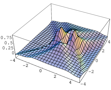
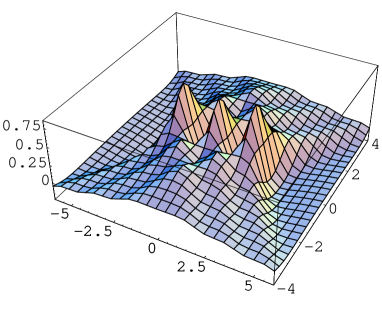
Figure 12: Two (left) / three (right) non-singular pairs of S-branes parallel in time.

Next we ask what happens if we arrange S-branes continuously in time. If we arrange the singular S-branes sources in time then we can create the usual static objects in this way. This is simple to see from the KG example. If we have the equation

$$(-\partial_{t}^{2}+\partial_{1}^{2}+\partial_{2}^{2}+\partial_{3}^{2})\phi=\delta(t-t_{0})\delta(x_{1})\delta(x_{2})\delta(x_{3})$$ (4.84)

and integrate both sides with respect to all values of $t_{0}$, then the right hand side becomes the three dimensional spatial delta function. This will also automatically produce the usual harmonic solution $\Phi=\int\!dt\ \phi=1/4\pi\sqrt{\vec{x}^{2}}$ to the Laplacian equation in three dimensions. In other words integrating an S-brane in time produces a pointlike static solution. It is also possible to create sources that begin and end in time, which are singular S-branes existing for finite time. Like the S-branes which exist for a moment in time, finite sources create light cone discontinuities starting and ending on the endpoints of the S-branes.

Having discussed the singular case, what static solutions we produce upon integrating imaginary sources in time? Take the four dimensional case where we must integrate

$$\int_{-\infty}^{\infty}\frac{dt_{0}}{-(t-t_{0}-is)^{2}+(x_{1})^{2}+(x_{2})^{2}+(x_{3})^{2}}.$$ (4.85)

The result is zero, for both of our four dimensional non-singular imaginary source solutions (1.14) and (1.20). This is technically because, for example for the latter solution, it takes both positive and negative values and integrating it over time gives zero. In addition this integral must be zero since otherwise we would have a non-singular static localized solitonic solution in four dimensions which is known to be impossible. Our result is therefore consistent. However as long as the solution is not infinitely extended in time (that is, the integral limits in (4.85) for the time-dependent solution are finite) then we generate an arbitrarily long-lived solution.

Another useful example is the partial integration of the “rolling tachyon” solution (4.78) which we take without loss of generality from $-t_{1}$ to $t_{1}$

$$\int_{-t_{1}}^{t_{1}}\!\!dt_{0}\;\phi(r,t-t_{0}) = \int_{-t_{1}}^{t_{1}}\!\!dt_{0}\;\frac{1}{r}\frac{C\pi}{2s}\left(\tanh\frac{\pi(r-t+t_{0})}{s}+\tanh\frac{\pi(r+t-t_{0})}{s}\right)$$ (4.86)

$$= \frac{C}{2r}\log\left[\frac{\cosh[2\pi(r+t_{1})/s]+\cosh[2\pi t/s]}{\cosh[2\pi(r-t_{1})/s]+\cosh[2\pi t/s]}\right].$$

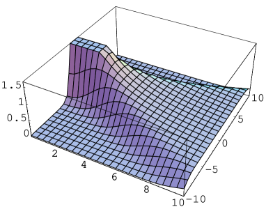
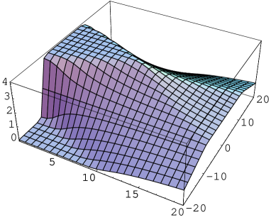
Figure 13: Left: Integrating the infinite array for a short period of time, $-5<t<5$, gives a solution similar to the un-integrated version. Right: Integrating the infinity array for $-10<t<10$, we find that the solution develops a nearly constant region near the origin of spacetime.

The spatial asymptotics are still like the un-integrated infinite array. As the array is integrated over longer periods of time, the potential near the origin becomes a constant as shown in Fig. 13.

4.2 Massive Klein-Gordon system

For a more explicit discussion, we here provide imaginary source solutions to massive Klein-Gordon theories in 1+1 and 1+2 dimensions.

For the Euclidean massive Klein-Gordon operator, we know the Green’s function in 3 dimensions

$$\phi=\frac{qe^{-mr}}{4\pi r}$$ (4.87)

is a solution of the equation of motion with a source,

$$(\partial_{i}^{2}-m^{2})\phi=q\delta^{3}(x_{i}),\quad(i=1,2,3),$$ (4.88)

where $m$ is the mass and $r$ is a radial variable in the 3 dimensional space. This can be used for getting a time-dependent solution in 1+2 dimensions. We can go ahead for getting imaginary source solutions by shifting the location of the source and performing the Wick rotation,

$$\phi=q\frac{\exp[-m\sqrt{(-it+s)^{2}+x^{2}+y^{2}}]}{\sqrt{(-it+s)^{2}+x^{2}+y^{2}}}.$$ (4.89)

For example, if we take the real part of the above solution, or in other words, we consider like charged sources located at $t=\pm s$, then we get a time-dependent solution

$$\phi=q\frac{e^{-mA}}{A^{2}+B^{2}}\left[A\cos(mB)-B\sin(mB)\right]$$ (4.90)

where $A$ (or $B$) is the real (or the imaginary) part of $\sqrt{(-it+s)^{2}+x^{2}+y^{2}}$,

$$A=\sqrt{(\Delta+\sqrt{\Delta^{2}+4s^{2}t^{2}})/2},\quad B=-st/A,\quad\Delta=-t^{2}+x^{2}+y^{2}+s^{2}.\hskip 14.22636pt$$ (4.91)

When an observer is spatially far from the light cone, i.e. when $-t^{2}+x^{2}+y^{2}\gg s^{2}$, then we may approximate $A\sim\sqrt{-t^{2}+x^{2}+y^{2}}$, so the solution looks like $\phi\sim q\exp[-m\sqrt{-t^{2}+x^{2}+y^{2}}]/\sqrt{-t^{2}+x^{2}+y^{2}}$. On the other hand, when $x^{2}+y^{2}\ll t^{2}-s^{2}$, we have $A\sim s$ and so $B\sim-t$. Thus the solution is oscillatory, $\phi\sim q\exp[-ms]\sin[-mt](1/t)$. Finally, if we take $s\gg(x,y,t)$ then the solution simplifies to the stationary wave $cos(mt)\ (e^{ms}/s)$. In sum, inside the light cone the solution is oscillating in time and thus looks almost like a plane wave with zero velocity, while outside of the light cone the solution is exponentially decaying asymptotically with length-scale given by proper distance from the lightcone, $\sqrt{-t^{2}+x^{2}+y^{2}}$. From the large $s$ limit we can see straightforwardly that imaginary sources will generate all the sourceless 1+2 massive Klein-Gordon solutions as all such solutions arise by Lorentz transformations of the stationary wave.

In the case of 1+1 dimensions, we start again by examining the Green’s function in 2 Euclidean dimensions. It has the modified second Bessel function solution

$$\phi(x,y)=-\frac{1}{2\pi}K_{1}(-m\sqrt{x^{2}+y^{2}})$$ (4.92)

which is exponentially decreasing at large radius and goes to infinity at the origin. Next take two such sources at $y=\pm is$ and perform the same Wick rotation $y\to it$. Taking the real and imaginary parts of the solution to get

$$\phi_{\rm R} = -\frac{1}{2\pi}{\rm Re}\left[K_{1}(-m\sqrt{x^{2}-(t-is)^{2}})\right],$$ (4.93)

$$\phi_{\rm I} = -\frac{1}{2\pi}{\rm Im}\left[K_{1}(-m\sqrt{x^{2}-(t-is)^{2}})\right],$$ (4.94)

we find nonsingular time dependent solutions to the massive Klein Gordon equations of motion as shown in Fig. 14.

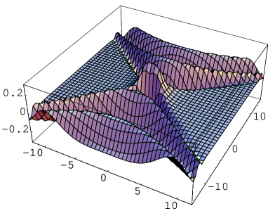
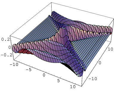
Figure 14: Left: 1+1 KG solution for two imaginary source at $t=\pm i$ and with the mass set to one, $m=1$. The ripples are in the forward and past light cones and create a lump at $t=0$. Right: Solution for two oppositely charged imaginary source at $t=\pm i$. The ripples are in the forward and past light cones and create a flat zero solution at $t=0$.

These solutions are asymptotically flat at large spatial directions and have damped oscillatory behavior in the past and future light cone. This oscillatory behavior is qualitatively different from the massless solutions with imaginary sources and reminiscent of the minisuperspace approximation for S-branes in string theory discussed in Ref. [8]. As with the massless KG case, these solutions are symmetric in space and either symmetric or antisymmetric in the time direction.

In the case of 1+0 dimension, a generic solution has been presented in Sec. 2.2.

4.3 Maxwell system

In this subsection we consider the Maxwell equations, another important physical system. We restrict our attention to 1+3 or 4 dimensional space(time). The Euclidean equations of motion are

$$\partial^{m}F_{mn}=0,$$ (4.95)

where $m,n=1,2,3,4$. We extend the coordinate $x_{4}$ to a complex variable $z_{4}\equiv x_{4}+ix_{0}$. As in the Klein-Gordon system, any solution to the above equations (with sources) can be extended to a solution of the complexified Maxwell equations by simply replacing $x_{4}$ in the solution by $z_{4}$. Restricting our attention to the $x_{4}=0$ subspace, we obtain the Lorentzian Maxwell equations

$$\partial^{\mu}F_{\mu\nu}=0$$ (4.96)

with $\mu,\nu=0,1,2,3$. Here note that we replaced the field $A_{4}$ by $A_{0}$ by the rule

$$A_{4}=-iA_{0},$$ (4.97)

which is necessary in accordance to the replacement $\partial/\partial z_{4}\rightarrow-i\partial/\partial x_{0}$ which was found in the general observation in the previous KG system. Due to this replacement, the metric in (4.96) is $(-1,1,1,1)$ and no $i$ appears in the equation.

To apply this procedure to obtain a new Lorentzian solution from a Euclidean solution, we have a further requirement that the resultant Lorentzian solution is real. Note that for this purpose we are allowed to solve the first Euclidean equation (4.95) with complex gauge fields.

4.3.1 Wick rotation of electrons: cylindrical waves

Let us present an explicit solution based on an electron-like solution in the Euclidean space. We adopt an ansatz $A_{1}=A_{2}=A_{4}=0$ for simplicity. Then the equations of motion of the Euclidean Maxwell system are just

$$(\partial_{1}^{2}+\partial_{2}^{2}+\partial_{4}^{2})A_{3}=0,\quad\partial_{3}A_{3}=0.$$ (4.98)

One example of the solutions is the electron-type, $A_{3}=C/\sqrt{x_{1}^{2}+x_{2}^{2}+x_{4}^{2}}$, which is an analog of a static electron potential, where a singular source is located at $x_{1}=x_{2}=x_{4}=0$. (The “real” electron can be obtained if we Wick rotate $A_{3}$ to $iA_{0}$.) Then the above Wick rotation procedure gives the following Lorentzian solution

$$A_{3}=\frac{C}{\sqrt{x_{1}^{2}+x_{2}^{2}-x_{0}^{2}}},\quad A_{1}=A_{2}=A_{0}=0.$$ (4.99)

This is a nontrivial time-dependent solution divergent at $x_{0}=\pm\sqrt{x_{1}^{2}+x_{2}^{2}}$. This divergence, which is linearly aligned along $x_{3}$, is propagating at the speed of light and lies on a light cone in the $(x_{0},x_{1},x_{2})$ spacetime.

We consider an imaginary-source extension of this solution to find nonsingular solutions. One might have already noticed that the situation is almost the same as the massless KG imaginary source solution in 1+2 dimensions (note that it is not 1+3 dimensions). After the Wick rotation for a pair of charges located at $x_{4}=ix_{0}=\pm s$, we obtain a Lorentzian solution $A_{0}=A_{1}=A_{3}=0$ with $A_{3}$ identified with $\phi$ in (3.56). Again from the combination in $\eta$ we expect a picture of colliding ripples as in the case of the massless KG system. Here however the solution is independent of $x_{3}$ and thus this is a colliding cylinder elongated along $x_{3}$ whose radius is shrinking ($x_{0}<0$) and growing ($x_{0}>0$) with the speed of light. We have an energy concentration only on this single cylinder whose radius is changing with speed of light, so this is a cylindrical “pulse”, rather than an oscillating wave. Translational symmetry of this solution along $x_{3}$ is reflected in the location of the imaginary sources. They are at $x_{0}=\pm is$, $x_{1}=x_{2}=0$ and the sources are homogeneously distributed along $x_{3}$.

Using the gauge field configuration obtained, we may compute the electric and magnetic fields. The non-vanishing components are $E_{3}$, $B_{1}$ and $B_{2}$. The configuration looks quite similar to a supertube in type II superstring theory — but in the present case of course there is no D2-brane to support the cylinder. One would expect that the cylinder should shrink with the speed of light, which does coincide with what we have calculated.

Another possibility is that, like the pair of the harmonic functions in (3.56), we could take opposite charges instead (or in other words, we could take an imaginary part of the complex solution for $A_{3}$). As in Sec. 4.1.2, we may consider a continuous array of these solutions in time. If we continuously arrange them in time and thus integrate the solutions over time, we get a nonzero constant. This is different from the result of Sec. 4.1.2, but this is still consistent with the fact that they do solve the equations of motion.

4.3.2 Wick rotation of monopoles

For the case of “electrons,” we implicitly made a double Wick rotation: first, in the usual electron solution we replaced the electrostatic potential by a Euclidean gauge field $A_{3}$, and then we made the Wick rotation for imaginary sources by replacing $A_{4}$ by $-iA_{0}$. We perform a similar analytic continuation for the Dirac monopoles. We start with embedding a Dirac monopole configuration into 4 dimensional Euclidean space as

$$A_{1}=\frac{-gx_{2}}{r(r+x_{4})},\quad A_{2}=\frac{gx_{1}}{r(r+x_{4})},\quad A_{3}=A_{4}=0,$$ (4.100)

where $r\equiv\sqrt{(x_{1})^{2}+(x_{2})^{2}+(x_{4})^{2}}$. The embedding is into the 3-subspace spanned by $(x_{1},x_{2},x_{4})$. Note that the Dirac string is at the negative axis of $x_{4}$. Then what we do is first to shift the origin of the monopole from $(0,0,0)$ to $(0,0,-s)$, and then to perform the Wick rotation $x_{4}\to ix_{0}$. After these operations, the Dirac string is located at $x_{1}=x_{2}=0$ and $ix_{0}<-s$. The important point here is that we shift the origin (the location of the source) in such a way that the Dirac string doesn’t appear in the real section of $(x_{0},x_{1},x_{2})$ spacetime. Taking the singular limit where $s=0$ however does need more than one gauge patch as the singularity now exists in real spacetime.

The gauge field $A_{4}$ becomes $-iA_{0}$ but this is vanishing from the first place. The nontrivial gauge fields $A_{1}$ and $A_{2}$ become complex, so we add (or subtract) their complex conjugate to make them real. Since we succeed in hiding the Dirac string completely in imaginary spacetime, the resultant configuration is everywhere regular. For example, we obtain

$$A_{1}=\frac{-gx_{2}}{r(r+s+ix_{0})}+{\rm c.c.}$$ (4.101)

where now $r=\sqrt{(x_{1})^{2}+(x_{2})^{2}-(x_{0})^{2}+s^{2}+2isx_{0}}$. One can easily see that this is nonsingular, because neither $r$ nor $r+s+ix_{0}$ can vanish for nonzero $s$.

Again, the obtained configuration is a cylindrical electro-magnetic wave (pulse), because the configuration does not depend on $x_{3}$.

4.3.3 Wick rotation of instantons: spherical waves

Next, let us take an Abelian instanton as a starting point. First we review this singular solutions in 4 dimensional Euclidean space. The gauge field of the solution is written as

$$A_{m}(x)=b_{mn}x_{n}h(r),\quad b\equiv\left(\begin{array}[]{cccc}0&1&0&0\\[-4.2679pt] -1&0&0&0\\[-4.2679pt] 0&0&0&1\\[-4.2679pt] 0&0&-1&0\end{array}\right),$$ (4.106)

where $r\equiv\sqrt{x_{1}^{2}+x_{2}^{2}+x_{3}^{2}+x_{4}^{2}}$. A straightforward computations show that

$$F_{12}=-2h(r)-(x_{1}^{2}+x_{2}^{2})h^{\prime}(r)/r,\quad F_{34}=-2h(r)-(x_{3}^{2}+x_{4}^{2})h^{\prime}(r)/r,$$

$$F_{13}=F_{24}=(x_{1}x_{4}-x_{2}x_{3})h^{\prime}(r)/r,\quad F_{23}=F_{41}=(x_{2}x_{4}-x_{1}x_{3})h^{\prime}(r)/r.$$

Thus the anti-self-duality equation $F_{mn}=-\frac{1}{2}\epsilon_{mnpq}F_{pq}$ can be satisfied if we require an equation $F_{12}=-F_{34}$ which is equivalent to $-4h(r)=\frac{h^{\prime}(r)}{r}$. This can be easily solved as

$$h(r)=\frac{C}{r^{4}}.$$ (4.107)

This is the Abelian instanton solution with a singularity at $r=0$.

The Wick rotation $x_{4}\rightarrow ix_{0}$ procedure gives a solution

$$A_{1}=x_{2}h(r),\quad A_{2}=-x_{1}h(r),\quad A_{3}=ix_{0}h(r),\quad A_{0}=-ix_{3}h(r),\quad$$ (4.108)

with the same $h(r)=C/r^{4}$ but now with $r\equiv\sqrt{x_{1}^{2}+x_{2}^{2}+x_{3}^{2}-x_{0}^{2}}$. In this solution, $A_{3}$ and $A_{0}$ are imaginary. To make a real solution, we may add a complex conjugate of the solution itself. When $C$ is real, the result is,

$$A_{1}=x_{2}\frac{2C}{r^{4}},\quad A_{2}=-x_{1}\frac{2C}{r^{4}},\quad A_{3}=A_{0}=0.$$ (4.109)

On the other hand, if we take imaginary $C=i\tilde{C}$ where $\tilde{C}$ is real, then

$$A_{1}=A_{2}=0,\quad A_{3}=-x_{0}\frac{2\tilde{C}}{r^{4}},\quad A_{0}=x_{3}\frac{2\tilde{C}}{r^{4}}.$$ (4.110)

These two solutions are both time dependent but still singular at the spacetime origin $r=0$. While the self-duality relation is broken when we added the complex conjugate, due to linearity the Maxwell equations of motion are still satisfied.

Let us move the singularity of the original Euclidean solution a little bit, as before, to regularize the solution. We start with the multiple instanton solution

$$A_{m}=\sum_{a=1}^{N}b_{mn}(x_{n}-\delta_{n4}s_{a})\frac{C_{a}}{(x_{1}^{2}+x_{2}^{2}+x_{3}^{2}+(x_{4}-s_{a})^{2})^{2}}.$$ (4.111)

The Wick rotation procedure produces a new Lorentzian solution

$$A_{1}=\sum_{a=1}^{N}\frac{C_{a}x_{2}}{(x_{1}^{2}+x_{2}^{2}+x_{3}^{2}+(ix_{0}\!-\!s_{a})^{2})^{2}},\quad A_{2}=\sum_{a=1}^{N}\frac{-C_{a}x_{1}}{(x_{1}^{2}+x_{2}^{2}+x_{3}^{2}+(ix_{0}\!-\!s_{a})^{2})^{2}},$$

$$A_{3}=\sum_{a=1}^{N}\frac{C_{a}(ix_{0}-s_{a})}{(x_{1}^{2}+x_{2}^{2}+x_{3}^{2}+(ix_{0}\!-\!s_{a})^{2})^{2}},\quad A_{0}=\sum_{a=1}^{N}\frac{-iC_{a}x_{3}}{(x_{1}^{2}+x_{2}^{2}+x_{3}^{2}+(ix_{0}\!-\!s_{a})^{2})^{2}}.$$

For simplicity we take a single location of a source ($N=1$), and add the complex conjugate to make the solution real. Supposing that $C$ is real, then we obtain a solution

$$A_{1}=\frac{2Cx_{2}(\Delta^{2}-4s^{2}x_{0}^{2})}{(\Delta^{2}+4s^{2}x_{0}^{2})^{2}},\quad A_{2}=\frac{-2Cx_{1}(\Delta^{2}-4s^{2}x_{0}^{2})}{(\Delta^{2}+4s^{2}x_{0}^{2})^{2}},$$

$$A_{3}=\frac{-2Cs(\Delta^{2}-4s^{2}x_{0}^{2}+4x_{0}^{2}\Delta^{2})}{(\Delta^{2}+4s^{2}x_{0}^{2})^{2}},\quad A_{0}=\frac{8Csx_{0}x_{3}\Delta}{(\Delta^{2}+4s^{2}x_{0}^{2})^{2}},$$ (4.112)

where $\Delta\equiv x_{1}^{2}+x_{2}^{2}+x_{3}^{2}-x_{0}^{2}+s^{2}$. It is easy to see that this is a regular configuration, because the denominator is always positive.

Let us look at a physical property of this time-dependent solution. The energy concentration of this time-dependent solution can be seen clearly in its asymptotic expansion in which the parameter $s$ in $\Delta$ is taken to be negligible, that is, $(-x_{0})^{2}+(x_{1})^{2}+(x_{2})^{2}+(x_{3})^{2})^{3}\gg s^{2}$. Physical field strengths have the following asymptotic values,

$$F_{12}=\frac{4C((x_{1})^{2}+(x_{2})^{2}-(x_{3})^{2}+(x_{0})^{2})}{((-x_{0})^{2}\!+\!(x_{1})^{2}\!+\!(x_{2})^{2}\!+\!(x_{3})^{2})^{3}},\quad F_{13}=\frac{8Cx_{2}x_{3}}{(-(x_{0})^{2}\!+\!(x_{1})^{2}\!+\!(x_{2})^{2}\!+\!(x_{3})^{2})^{3}},$$

$$F_{23}=\frac{-8Cx_{1}x_{3}}{(-(x_{0})^{2}\!+\!(x_{1})^{2}\!+\!(x_{2})^{2}\!+\!(x_{3})^{2})^{3}},\quad F_{01}=\frac{8Cx_{2}x_{0}}{(-(x_{0})^{2}\!+\!(x_{1})^{2}\!+\!(x_{2})^{2}\!+\!(x_{3})^{2})^{3}},$$

$$F_{02}=\frac{-8Cx_{1}x_{0}}{(-(x_{0})^{2}\!+\!(x_{1})^{2}\!+\!(x_{2})^{2}\!+\!(x_{3})^{2})^{3}},\quad F_{03}=0.$$ (4.113)

Note that all the entries have a Lorentz invariant length in their denominators. Therefore the solution (4.112) describes a 2-sphere contracting and expanding with the speed of light — the solution is specified by $\Delta$ and if one looks at an equal $\Delta$ surface one can recognize this geometrical picture.

Let us see what happens at $x_{0}=0$. In the solution, $A_{0}$ vanishes, and resultantly the electric field vanishes; there is a magnetic field, locally concentrated near the origin $x_{1}=x_{2}=x_{3}=0$. We have plotted some of the gauge field strengths a little after the collision incident $x_{0}=0$, in Fig. 15. After a long while, the spherical wave (pulse) expands, as seen in Fig. 16.

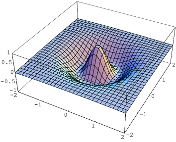
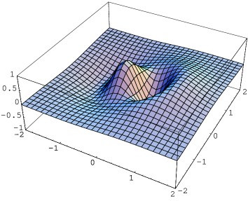
Figure 15: Left: the magnetic field $F_{12}$ of the solution (4.112) at a time slice a little after the collision $x_{0}=0$, in a 2 dimensional slice $x_{3}=0$. Right: the magnetic field $F_{13}$ at the same time and slice. This component vanishes at $x_{0}=0$.

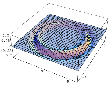
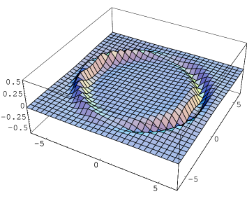
Figure 16: Left: The field strength $F_{12}$ long time after the collision. One can see that the spherical wave (pulse) expands. Right: The same can be observed for the component $F_{13}$. But the amplitudes of the waves are small, which is consistent with the conservation of the energy.

One may think of $C$ as a pure imaginary constant, before adding the complex conjugate. Then the resultant solution is different from (4.112). This can be thought of as “dual” of the solution (4.112), because at the collision incidence $x_{0}=0$, the electric field is nonzero while the magnetic field vanishes. In these solutions there is a close and fascinating relationship between electric magnetic duality and analytic continuation. This is seen for example in Eqs. (4.109) and (4.110) which can be thought of as related by analytic continuation. From a short calculation one finds that these give rise to field strengths dual to each other. For example, $F_{03}$ of (4.110) is equal to $F_{12}$ of (4.109) if we identify $C=-\tilde{C}$. This is similar then to the usual case of electric magnetic duality however here we see that it applies to a new class of solutions coming from analytic continuations of the instanton.

Of course, $C$ can be an arbitrary complex constant, and thus there can be a mixture of these electric and magnetic collisions. Infinite arrays of such Abelian instantons can also be explicitly summed just like in the Klein-Gordon case using the same hyperbolic tangent formulas. The resulting solution is similar to a time dependent dyon.

5 Further Generalizations

In this paper we have developed the utility of complexified spacetime and its imaginary sources. While it is unusual to think of fluctuations of fields to be related to anything else but physically accessible real spacetime objects, we conclude that complexification of spacetime is a useful viewpoint. Our main results include the proof that imaginary source configurations can be thought to be a new way to understand solutions to homogeneous differential equations since we are able to prove in several classes of theories that every smooth solution has at least one corresponding imaginary source configuration. In mathematical terms our result can be viewed in the linear cases as unifying the analysis of singular and non-singular solutions to differential equations by extending Green’s function techniques. Therefore we expect the methods of imaginary sources to be a useful and practical tool in many other settings both linear and nonlinear. The following applications might be interesting,

• Non-Abelian gauge theory                  $\bullet$ Dirac-Born-Infeld theory

• Gravity                                               $\bullet$ String theory

as all are nonlinear in equations and so the reality condition will be difficult to be satisfied. But it is possible that in special examples the reality can be ensured. For example in the case of gravity, this should be explicitly possible in all Weyl type ansatzes. In string theory, imaginary D-branes in pairs [2, 3, 4] or odd numbers [5] do give rise to sensible backgrounds. From our discussion it is clear that imaginary D-branes do not exhaust the physical closed string backgrounds even at the linear massless level. To produce independent dilaton and gauge field configurations, at minimum it is necessary to use non-BPS imaginary D-branes. The notion of imaginary strings must also be developed to produce the source free background B-fields. A notion of imaginary strings is in fact probably already necessary to understand the dynamics of imaginary D-branes.

To what extent are our current results related to such nonlinear theories. In this paper we provided proofs of the completeness of the imaginary sources even for the Maxwell system. One should note that the Klein-Gordon equation arises in many important cases such as the linearizations of gravity and string theory. To the extent that we trust that the linear approximations have corresponding nonlinear exact solutions, we have proved that imaginary sources are relevant in gravity and string theory. However this is not so straightforward. One might argue that in nonlinear theories such as field theories with nontrivial interaction terms there will be no notion of “basis” because field configurations can not simply be added together to produce a new configuration. We hope though that S-charges associated to given time-dependent solutions (when the completeness conjecture is correct it always exists) would be an interesting and intrinsic ways to characterize field configurations.

In addition to understanding the realm of applicability of the imaginary source conjecture in other theories, there are many interesting directions to pursue. For example in gravitational theories one should develop the notion of ADM S-mass. One can also try to describe the interaction of imaginary sources with each other and real sources. Describing such processes would in fact lead to an alternate interpretation of positron electron annihilation. Such unusual interactions between imaginary sources and real sources should arise since we have shown asymptotically they can have the same mass and charge so these quantum numbers can be conserved in interactions. A further natural question is can one generalize the notion of spontaneous symmetry breaking to the case of imaginary source solutions. This would include the development of solutions where the delta functions can be field dependent and take imaginary values in contrast to delta functions which are just spacetime dependent. Moreover, the arrays infinitely extended in time give rise to constant field configurations. If one could produce similar imaginary D-branes extended in time, they might be a useful clue to describing field theory duals to gravity theories in flat space. Finally it should be interesting to understand if notions such as T-duality are applicable to the case of imaginary sources.

Acknowledgements           K. H. would like to thank G. W. Gibbons for fruitful discussions and valuable comments. The work of K. H. is supported in part by the National Science Foundation under Grant No. PHY99-07949, by the Japan Society for Promotion of Science, and by the Royal Society International Grants. J. E. W. is supported in part by the National Science Council under the NSC grant number NSC 94-2119-M-002-001 and by the National Center for Theoretical Sciences.

References

- [1] A. Sen, “Rolling Tachyon,” JHEP 0204 (2002) 048, hep-th/0203211; “Tachyon Matter,” hep-th/0203265; “Field Theory of Tachyon Matter,” Mod. Phys. Lett. A17 (2002) 1797, hep-th/0204143.
- [2] A. Maloney, A. Strominger and X. Yin, “Sbrane Thermodynamics,” JHEP 0310 (2003) 048, hep-th/0302146.
- [3] D. Gaiotto, N. Itzhai and L. Rastelli, “Closed Strings as Imaginary D-branes,” Nucl. Phys. B688 (2004) 70, hep-th/0304192.
- [4] G. Jones, A. Maloney and A. Strominger, ”Nonsingular solutions for S-branes,” Phys. Rev. D69 (2004) 126008, hep-th/0403050.
- [5] G. Jones and J. E. Wang, ”Weyl Card Diagrams and new S-brane Solutions of Gravity,” hep-th/0409070.
-
[6]
J. E. Wang, “Twisting S-branes,” JHEP 0405 (2004) 066,
hep-th/0403094;
G. Tasinato, I. Zavala, C. P. Burgess and F. Quevedo, “Regular S-brane Backgrounds”, JHEP 0406 (2004) 015, hep-th/0403156;
H. Lu and J. F. Vazquez-Poritz, “Nonsingular Twisted S-branes from Rotating Branes,” JHEP 0407 (2004) 050. - [7] M. Gutperle and A. Strominger, “Spacelike Branes,” JHEP 0204 (2002) 018, hep-th/0202210.
-
[8]
A. Strominger, “Open String Creation by S-Branes,”
hep-th/0209090;